Lecture 11: Polarized Light

Outline

1 Fundamentals of Polarized Light2 Descriptions of Polarized Light3 Scattering Polarization4 Zeeman Effect5 Hanle Effect

Fundamentals of Polarized Light

Electromagnetic Waves in Matter

electromagnetic waves are a direct consequence of Maxwell’sequations

optics: interaction of electromagnetic waves with matter asdescribed by material equations

polarization properties of electromagnetic waves are integral partof optics

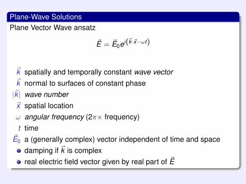
Plane-Wave SolutionsPlane Vector Wave ansatz

~E = ~E0ei(~k ·~x−ωt)

~k spatially and temporally constant wave vector~k normal to surfaces of constant phase|~k | wave number~x spatial locationω angular frequency (2π× frequency)t time

~E0 a (generally complex) vector independent of time and spacedamping if ~k is complexreal electric field vector given by real part of ~E

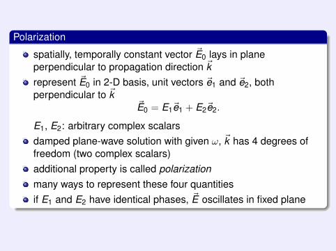
Polarization

spatially, temporally constant vector ~E0 lays in planeperpendicular to propagation direction ~krepresent ~E0 in 2-D basis, unit vectors ~e1 and ~e2, bothperpendicular to ~k

~E0 = E1~e1 + E2~e2.

E1, E2: arbitrary complex scalarsdamped plane-wave solution with given ω, ~k has 4 degrees offreedom (two complex scalars)additional property is called polarizationmany ways to represent these four quantitiesif E1 and E2 have identical phases, ~E oscillates in fixed plane

Description of Polarized Light

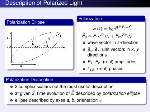
Polarization EllipsePolarization

~E (t) = ~E0ei(~k ·~x−ωt)

~E0 = E1eiδ1~ex + E2eiδ2~ey

wave vector in z-direction~ex , ~ey : unit vectors in x , ydirectionsE1, E2: (real) amplitudesδ1,2: (real) phases

Polarization Description2 complex scalars not the most useful descriptionat given ~x , time evolution of ~E described by polarization ellipseellipse described by axes a, b, orientation ψ

Jones Formalism

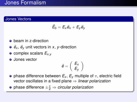
Jones Vectors

~E0 = Ex~ex + Ey~ey

beam in z-direction~ex , ~ey unit vectors in x , y -directioncomplex scalars Ex ,y

Jones vector~e =

(ExEy

)phase difference between Ex , Ey multiple of π, electric fieldvector oscillates in a fixed plane⇒ linear polarizationphase difference ±π

2 ⇒ circular polarization

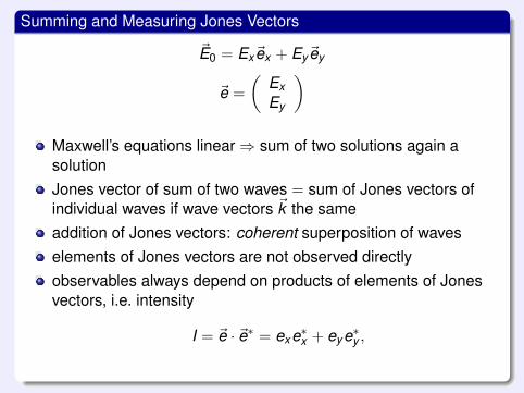
Summing and Measuring Jones Vectors

~E0 = Ex~ex + Ey~ey

~e =

(ExEy

)

Maxwell’s equations linear⇒ sum of two solutions again asolutionJones vector of sum of two waves = sum of Jones vectors ofindividual waves if wave vectors ~k the sameaddition of Jones vectors: coherent superposition of waveselements of Jones vectors are not observed directlyobservables always depend on products of elements of Jonesvectors, i.e. intensity

I = ~e · ~e∗ = exe∗x + eye∗y ,

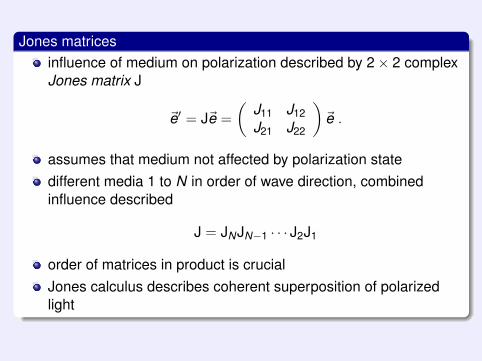
Jones matricesinfluence of medium on polarization described by 2× 2 complexJones matrix J

~e′ = J~e =

(J11 J12J21 J22

)~e .

assumes that medium not affected by polarization statedifferent media 1 to N in order of wave direction, combinedinfluence described

J = JNJN−1 · · · J2J1

order of matrices in product is crucialJones calculus describes coherent superposition of polarizedlight

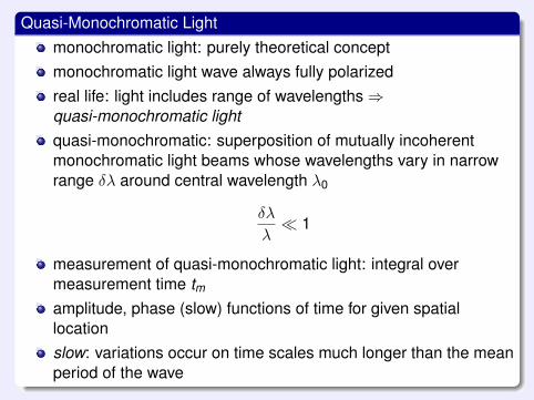
Quasi-Monochromatic Lightmonochromatic light: purely theoretical conceptmonochromatic light wave always fully polarizedreal life: light includes range of wavelengths⇒quasi-monochromatic lightquasi-monochromatic: superposition of mutually incoherentmonochromatic light beams whose wavelengths vary in narrowrange δλ around central wavelength λ0

δλ

λ� 1

measurement of quasi-monochromatic light: integral overmeasurement time tmamplitude, phase (slow) functions of time for given spatiallocationslow: variations occur on time scales much longer than the meanperiod of the wave

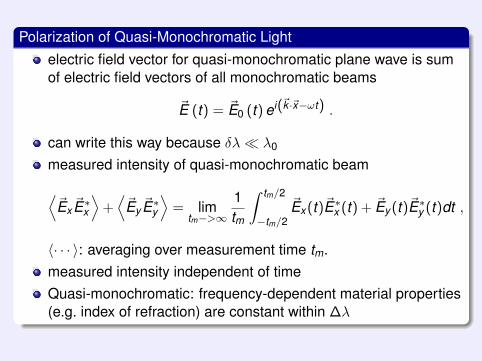
Polarization of Quasi-Monochromatic Light

electric field vector for quasi-monochromatic plane wave is sumof electric field vectors of all monochromatic beams

~E (t) = ~E0 (t) ei(~k ·~x−ωt) .

can write this way because δλ� λ0

measured intensity of quasi-monochromatic beam⟨~Ex ~E∗x

⟩+⟨~Ey ~E∗y

⟩= lim

tm−>∞

1tm

∫ tm/2

−tm/2

~Ex (t)~E∗x (t) + ~Ey (t)~E∗y (t)dt ,

〈· · · 〉: averaging over measurement time tm.measured intensity independent of timeQuasi-monochromatic: frequency-dependent material properties(e.g. index of refraction) are constant within ∆λ

Stokes and Mueller Formalisms

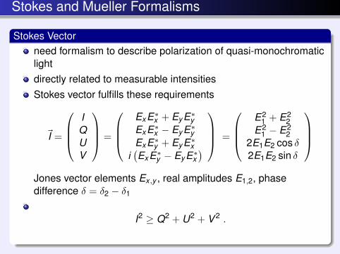
Stokes Vectorneed formalism to describe polarization of quasi-monochromaticlightdirectly related to measurable intensitiesStokes vector fulfills these requirements

~I =

IQUV

=

ExE∗x + EyE∗yExE∗x − EyE∗yExE∗y + EyE∗x

i(ExE∗y − EyE∗x

) =

E2

1 + E22

E21 − E2

22E1E2 cos δ2E1E2 sin δ

Jones vector elements Ex ,y , real amplitudes E1,2, phasedifference δ = δ2 − δ1

I2 ≥ Q2 + U2 + V 2 .

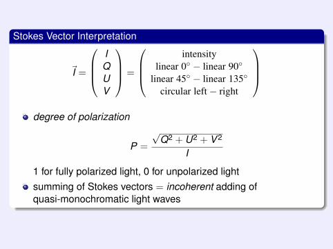
Stokes Vector Interpretation

~I =

IQUV

=

intensity

linear 0◦ − linear 90◦

linear 45◦ − linear 135◦

circular left− right

degree of polarization

P =

√Q2 + U2 + V 2

I

1 for fully polarized light, 0 for unpolarized lightsumming of Stokes vectors = incoherent adding ofquasi-monochromatic light waves

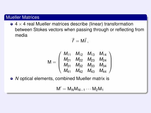
Mueller Matrices4× 4 real Mueller matrices describe (linear) transformationbetween Stokes vectors when passing through or reflecting frommedia

~I′ = M~I ,

M =

M11 M12 M13 M14M21 M22 M23 M24M31 M32 M33 M34M41 M42 M43 M44

N optical elements, combined Mueller matrix is

M′ = MNMN−1 · · ·M2M1

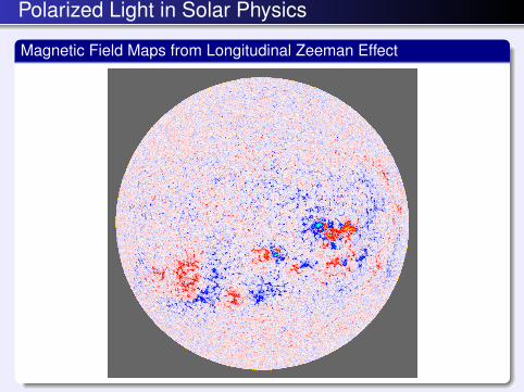
Polarized Light in Solar Physics

Magnetic Field Maps from Longitudinal Zeeman Effect

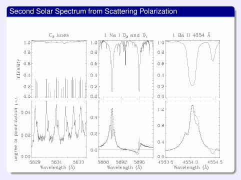
Second Solar Spectrum from Scattering Polarization

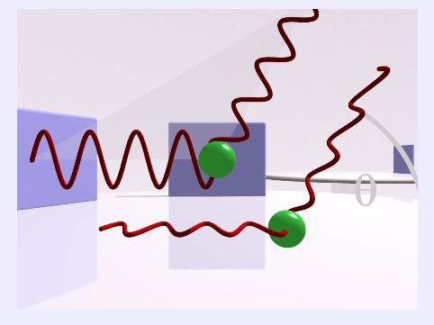
Scattering Polarization

Single Particle Scatteringlight is absorbed and re-emittedif light has low enough energy, no energy transfered to electron,but photon changes direction⇒ elastic scatteringfor high enough energy, photon transfers energy onto electron⇒inelastic (Compton) scatteringThomson scattering on free electronsRayleigh scattering on bound electronsbased on very basic physics, scattered light is linearly polarized

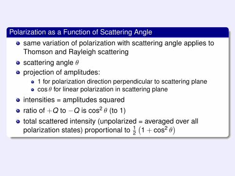
Polarization as a Function of Scattering Angle

same variation of polarization with scattering angle applies toThomson and Rayleigh scatteringscattering angle θprojection of amplitudes:

1 for polarization direction perpendicular to scattering planecos θ for linear polarization in scattering plane

intensities = amplitudes squaredratio of +Q to −Q is cos2 θ (to 1)total scattered intensity (unpolarized = averaged over allpolarization states) proportional to 1

2

(1 + cos2 θ

)

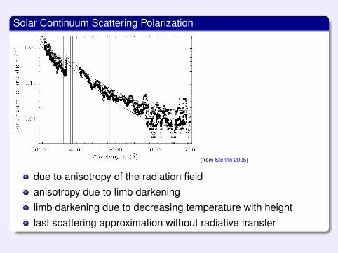
Solar Continuum Scattering Polarization

(from Stenflo 2005)

due to anisotropy of the radiation fieldanisotropy due to limb darkeninglimb darkening due to decreasing temperature with heightlast scattering approximation without radiative transfer

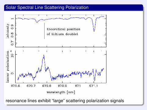
Solar Spectral Line Scattering Polarization

resonance lines exhibit “large” scattering polarization signals

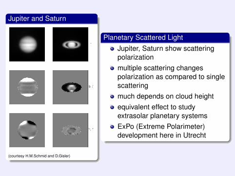
Jupiter and Saturn

(courtesy H.M.Schmid and D.Gisler)

Planetary Scattered Light

Jupiter, Saturn show scatteringpolarizationmultiple scattering changespolarization as compared to singlescatteringmuch depends on cloud heightequivalent effect to studyextrasolar planetary systemsExPo (Extreme Polarimeter)development here in Utrecht

Zeeman Effect

photos.aip.org/

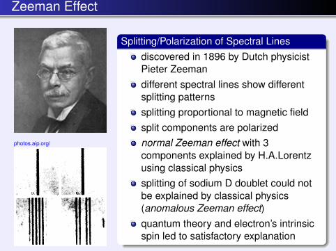
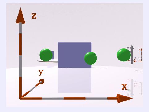
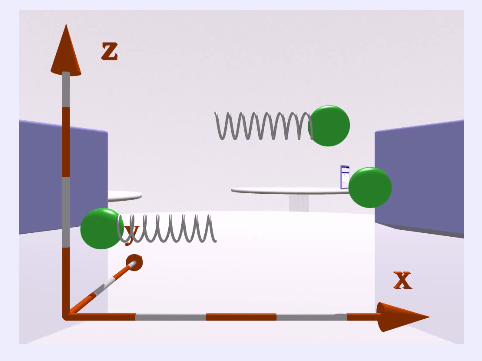
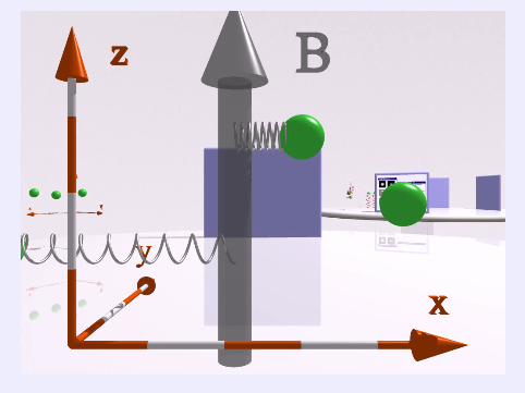
Splitting/Polarization of Spectral Linesdiscovered in 1896 by Dutch physicistPieter Zeemandifferent spectral lines show differentsplitting patternssplitting proportional to magnetic fieldsplit components are polarizednormal Zeeman effect with 3components explained by H.A.Lorentzusing classical physicssplitting of sodium D doublet could notbe explained by classical physics(anomalous Zeeman effect)quantum theory and electron’s intrinsicspin led to satisfactory explanation

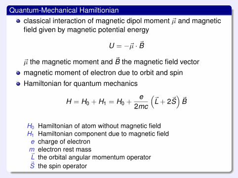
Quantum-Mechanical Hamiltionianclassical interaction of magnetic dipol moment ~µ and magneticfield given by magnetic potential energy

U = −~µ · ~B

~µ the magnetic moment and ~B the magnetic field vectormagnetic moment of electron due to orbit and spinHamiltonian for quantum mechanics

H = H0 + H1 = H0 +e

2mc

(~L + 2~S

)~B

H0 Hamiltonian of atom without magnetic fieldH1 Hamiltonian component due to magnetic field

e charge of electronm electron rest mass~L the orbital angular momentum operator~S the spin operator

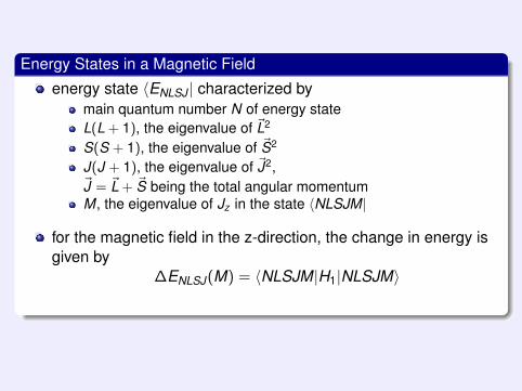
Energy States in a Magnetic Field

energy state 〈ENLSJ | characterized bymain quantum number N of energy stateL(L + 1), the eigenvalue of ~L2

S(S + 1), the eigenvalue of ~S2

J(J + 1), the eigenvalue of ~J2,~J = ~L + ~S being the total angular momentumM, the eigenvalue of Jz in the state 〈NLSJM|

for the magnetic field in the z-direction, the change in energy isgiven by

∆ENLSJ(M) = 〈NLSJM|H1|NLSJM〉

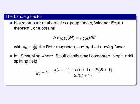
The Landé g Factor

based on pure mathematics (group theory, Wiegner Eckarttheorem), one obtains

∆ENLSJ(M) = µ0gLBM

with µ0 = e~2m the Bohr magneton, and gL the Landé g-factor

in LS coupling where B sufficiently small compared to spin-orbitsplitting field

gL = 1 +J(J + 1) + L(L + 1)− S(S + 1)

2J(J + 1)

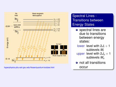
hyperphysics.phy-astr.gsu.edu/hbase/quantum/sodzee.html

Spectral Lines -Transitions betweenEnergy States

spectral lines aredue to transitionsbetween energystates:

lower level with 2Jl + 1sublevels Ml

upper level with 2Ju + 1sublevels Mu

not all transitionsoccur

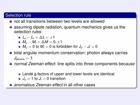
Selection rulenot all transitions between two levels are allowedassuming dipole radiation, quantum mechanics gives us theselection rules:

Lu − Ll = ∆L = ±1Mu −Ml = ∆M = 0,±1Mu = 0 to Ml = 0 is forbidden for Ju − Jl = 0

total angular momentum conservation: photon always carriesJphoton = 1normal Zeeman effect: line splits into three components because

Landé g-factors of upper and lower levels are identicalJu = 1 to Jl = 0 transition

anomalous Zeeman effect in all other cases

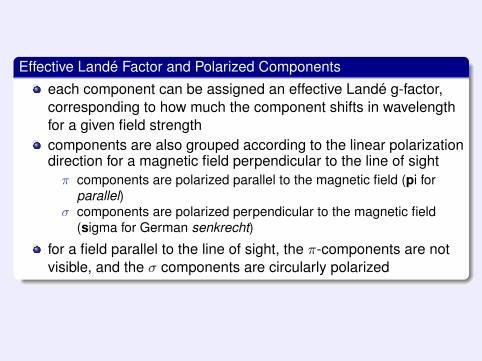
Effective Landé Factor and Polarized Componentseach component can be assigned an effective Landé g-factor,corresponding to how much the component shifts in wavelengthfor a given field strengthcomponents are also grouped according to the linear polarizationdirection for a magnetic field perpendicular to the line of sightπ components are polarized parallel to the magnetic field (pi for

parallel)σ components are polarized perpendicular to the magnetic field

(sigma for German senkrecht)

for a field parallel to the line of sight, the π-components are notvisible, and the σ components are circularly polarized

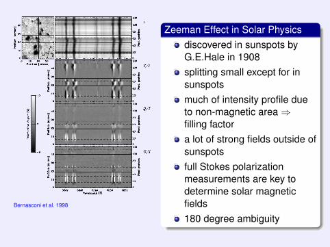
Bernasconi et al. 1998

Zeeman Effect in Solar Physicsdiscovered in sunspots byG.E.Hale in 1908splitting small except for insunspotsmuch of intensity profile dueto non-magnetic area⇒filling factora lot of strong fields outside ofsunspotsfull Stokes polarizationmeasurements are key todetermine solar magneticfields180 degree ambiguity

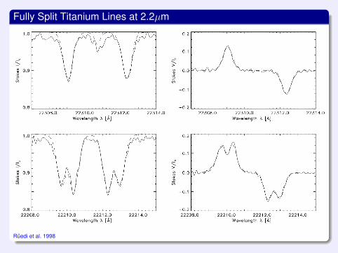
Fully Split Titanium Lines at 2.2µm

Rüedi et al. 1998

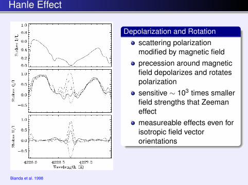
Hanle Effect

Bianda et al. 1998

Depolarization and Rotationscattering polarizationmodified by magnetic fieldprecession around magneticfield depolarizes and rotatespolarizationsensitive ∼ 103 times smallerfield strengths that Zeemaneffectmeasureable effects even forisotropic field vectororientations