Derived-term Automata forExtended Weighted Rational Expressions

Akim Demaille (2016-05-04 11:15:06 +0200 ab706b4)

LRDE, EPITA, akim@lrde.epita.fr

Contents

1 Introduction 2

2 Notations 32.1 Rational Series . . . . . . . . . . . . . . . . . . . . . . . . . . . . . . . . . . . 32.2 Extended Weighted Rational Expressions . . . . . . . . . . . . . . . . . . . . 42.3 Rational Polynomials . . . . . . . . . . . . . . . . . . . . . . . . . . . . . . . . 52.4 Rational Expansions . . . . . . . . . . . . . . . . . . . . . . . . . . . . . . . . 62.5 Weighted Automata . . . . . . . . . . . . . . . . . . . . . . . . . . . . . . . . 7

3 Computing Expansions of Expressions 83.1 Expansion of a Rational Expression . . . . . . . . . . . . . . . . . . . . . . . 83.2 Connection with Derivatives . . . . . . . . . . . . . . . . . . . . . . . . . . . . 9

4 Expansion-Based Derived-Term Automaton 94.1 Deterministic Automata . . . . . . . . . . . . . . . . . . . . . . . . . . . . . . 114.2 The Case of Complement . . . . . . . . . . . . . . . . . . . . . . . . . . . . . 124.3 Complexity and Performances . . . . . . . . . . . . . . . . . . . . . . . . . . . 12

5 Related Work 13

6 Conclusion 14

A Appendix 15

B Appendix: Proof of Theorem 20 16B.1 Derivation by Words . . . . . . . . . . . . . . . . . . . . . . . . . . . . . . . . 16B.2 Derived Terms . . . . . . . . . . . . . . . . . . . . . . . . . . . . . . . . . . . 19B.3 Derived-term Automaton . . . . . . . . . . . . . . . . . . . . . . . . . . . . . 21

AbstractWe present an algorithm to build an automaton from a rational expression. This approachintroduces support for extended weighted expressions. Inspired by derived-term based algorithms,its core relies on a different construct, rational expansions. We introduce an inductive algorithmto compute the expansion of an expression from which the automaton follows. This algorithmis independent of the size of the alphabet, and actually even supports infinite alphabets. Itcan easily be accommodated to generate deterministic (weighted) automata. These constructsare implemented in Vcsn, a free-software platform dedicated to weighted automata and rationalexpressions.

licensed under Creative Commons License CC-BYLeibniz International Proceedings in InformaticsSchloss Dagstuhl – Leibniz-Zentrum für Informatik, Dagstuhl Publishing, Germany

arX

iv:1

605.

0153

0v1

[cs

.FL

] 5

May

201

6

2 CONTENTS

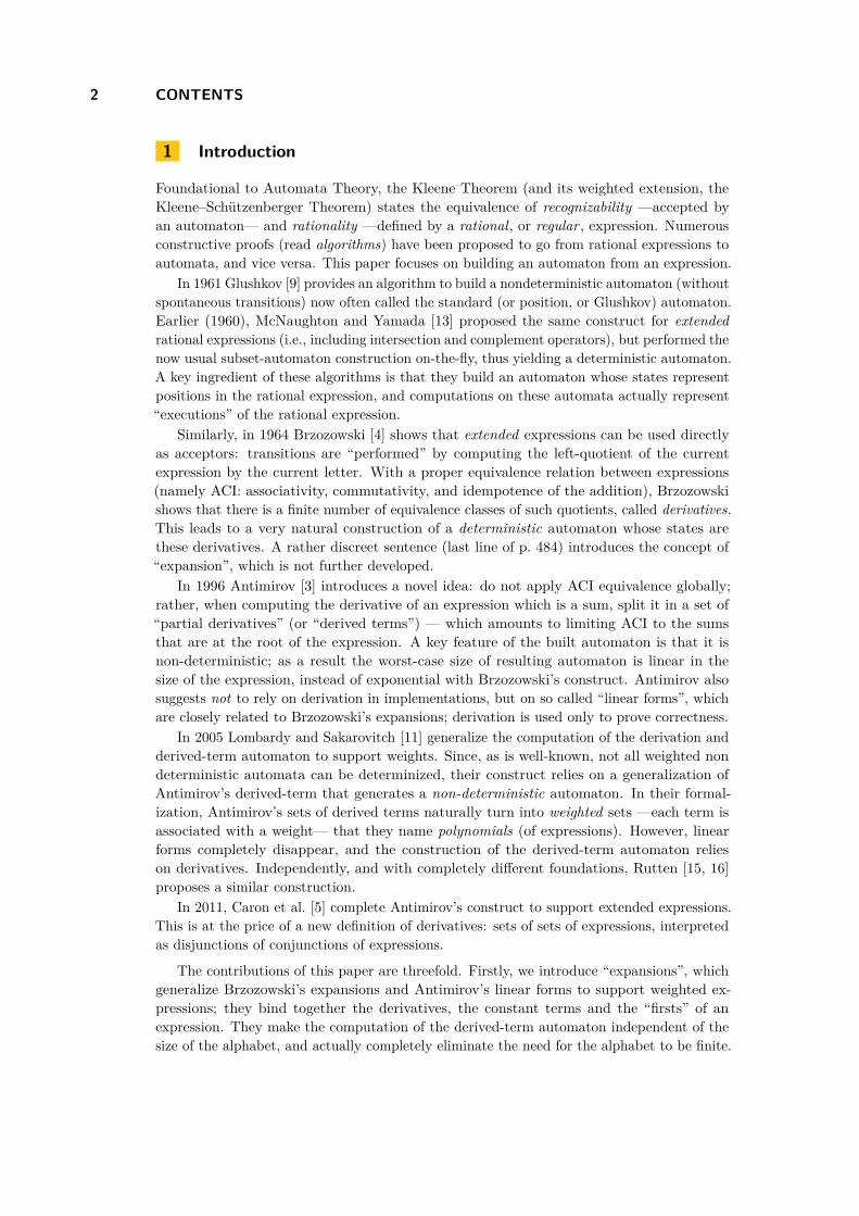
1 Introduction

Foundational to Automata Theory, the Kleene Theorem (and its weighted extension, theKleene–Schützenberger Theorem) states the equivalence of recognizability —accepted byan automaton— and rationality —defined by a rational, or regular , expression. Numerousconstructive proofs (read algorithms) have been proposed to go from rational expressions toautomata, and vice versa. This paper focuses on building an automaton from an expression.

In 1961 Glushkov [9] provides an algorithm to build a nondeterministic automaton (withoutspontaneous transitions) now often called the standard (or position, or Glushkov) automaton.Earlier (1960), McNaughton and Yamada [13] proposed the same construct for extendedrational expressions (i.e., including intersection and complement operators), but performed thenow usual subset-automaton construction on-the-fly, thus yielding a deterministic automaton.A key ingredient of these algorithms is that they build an automaton whose states representpositions in the rational expression, and computations on these automata actually represent“executions” of the rational expression.

Similarly, in 1964 Brzozowski [4] shows that extended expressions can be used directlyas acceptors: transitions are “performed” by computing the left-quotient of the currentexpression by the current letter. With a proper equivalence relation between expressions(namely ACI: associativity, commutativity, and idempotence of the addition), Brzozowskishows that there is a finite number of equivalence classes of such quotients, called derivatives.This leads to a very natural construction of a deterministic automaton whose states arethese derivatives. A rather discreet sentence (last line of p. 484) introduces the concept of“expansion”, which is not further developed.

In 1996 Antimirov [3] introduces a novel idea: do not apply ACI equivalence globally;rather, when computing the derivative of an expression which is a sum, split it in a set of“partial derivatives” (or “derived terms”) — which amounts to limiting ACI to the sumsthat are at the root of the expression. A key feature of the built automaton is that it isnon-deterministic; as a result the worst-case size of resulting automaton is linear in thesize of the expression, instead of exponential with Brzozowski’s construct. Antimirov alsosuggests not to rely on derivation in implementations, but on so called “linear forms”, whichare closely related to Brzozowski’s expansions; derivation is used only to prove correctness.

In 2005 Lombardy and Sakarovitch [11] generalize the computation of the derivation andderived-term automaton to support weights. Since, as is well-known, not all weighted nondeterministic automata can be determinized, their construct relies on a generalization ofAntimirov’s derived-term that generates a non-deterministic automaton. In their formal-ization, Antimirov’s sets of derived terms naturally turn into weighted sets —each term isassociated with a weight— that they name polynomials (of expressions). However, linearforms completely disappear, and the construction of the derived-term automaton relieson derivatives. Independently, and with completely different foundations, Rutten [15, 16]proposes a similar construction.

In 2011, Caron et al. [5] complete Antimirov’s construct to support extended expressions.This is at the price of a new definition of derivatives: sets of sets of expressions, interpretedas disjunctions of conjunctions of expressions.

The contributions of this paper are threefold. Firstly, we introduce “expansions”, whichgeneralize Brzozowski’s expansions and Antimirov’s linear forms to support weighted ex-pressions; they bind together the derivatives, the constant terms and the “firsts” of anexpression. They make the computation of the derived-term automaton independent of thesize of the alphabet, and actually completely eliminate the need for the alphabet to be finite.

CONTENTS 3

Secondly, we provide support for extended weighted rational expressions, which generalizesboth Lombardy and Sakarovitch [11] and Caron et al. [5]. And thirdly, we introduce avariation of this algorithm to build deterministic (weighted) automata.

We first settle the notations in Sect. 2, provide an algorithm to compute the expansion ofan expression in Sect. 3, which is used in Sect. 4 to propose an alternative construction ofthe derived-term automaton. In Sect. 5 we expose related work and conclude in Sect. 6.

Interested readers may experiment with the concepts introduced here using Vcsn. Vcsnis a free-software platform dedicated to weighted automata and rational expressions [8]. Itsupports both derivations and expansions, as exposed in this paper, and the correspondingconstructions of the derived-term automaton1.

2 Notations

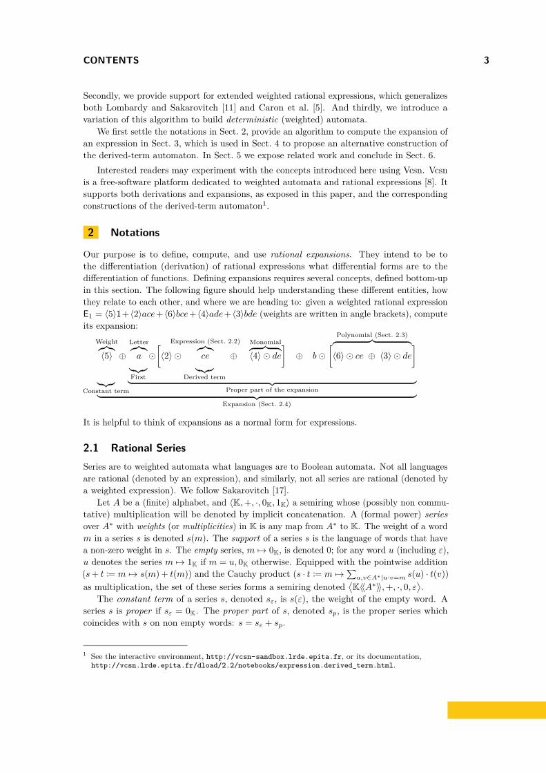
Our purpose is to define, compute, and use rational expansions. They intend to be tothe differentiation (derivation) of rational expressions what differential forms are to thedifferentiation of functions. Defining expansions requires several concepts, defined bottom-upin this section. The following figure should help understanding these different entities, howthey relate to each other, and where we are heading to: given a weighted rational expressionE1 = 〈5〉1+ 〈2〉ace+ 〈6〉bce+ 〈4〉ade+ 〈3〉bde (weights are written in angle brackets), computeits expansion:

Weight︷︸︸︷〈5〉

︸︷︷︸Constant term

⊕Letter︷︸︸︷a︸︷︷︸

First

�[〈2〉 �

Expression (Sect. 2.2)︷︸︸︷ce︸︷︷︸

Derived term

⊕Monomial︷ ︸︸ ︷〈4〉 � de

]⊕ b�

[ Polynomial (Sect. 2.3)︷ ︸︸ ︷〈6〉 � ce ⊕ 〈3〉 � de

]︸ ︷︷ ︸

Proper part of the expansion︸ ︷︷ ︸Expansion (Sect. 2.4)

It is helpful to think of expansions as a normal form for expressions.

2.1 Rational SeriesSeries are to weighted automata what languages are to Boolean automata. Not all languagesare rational (denoted by an expression), and similarly, not all series are rational (denoted bya weighted expression). We follow Sakarovitch [17].

Let A be a (finite) alphabet, and 〈K,+, ·, 0K, 1K〉 a semiring whose (possibly non commu-tative) multiplication will be denoted by implicit concatenation. A (formal power) seriesover A∗ with weights (or multiplicities) in K is any map from A∗ to K. The weight of a wordm in a series s is denoted s(m). The support of a series s is the language of words that havea non-zero weight in s. The empty series, m 7→ 0K, is denoted 0; for any word u (including ε),u denotes the series m 7→ 1K if m = u, 0K otherwise. Equipped with the pointwise addition(s+ t := m 7→ s(m) + t(m)) and the Cauchy product (s · t := m 7→

∑u,v∈A∗|u·v=m s(u) · t(v))

as multiplication, the set of these series forms a semiring denoted⟨K〈〈A∗〉〉,+, ·, 0, ε

⟩.

The constant term of a series s, denoted sε, is s(ε), the weight of the empty word. Aseries s is proper if sε = 0K. The proper part of s, denoted sp, is the proper series whichcoincides with s on non empty words: s = sε + sp.

1 See the interactive environment, http://vcsn-sandbox.lrde.epita.fr, or its documentation,http://vcsn.lrde.epita.fr/dload/2.2/notebooks/expression.derived_term.html.

4 CONTENTS

The star of a series is an infinite sum: s∗ :=∑

n∈N sn. To ensure semantic soundness,

we suppose that K is a topological semiring, i.e., it is equipped with a topology, and bothaddition and multiplication are continuous. Besides, it is supposed to be strong, i.e., theproduct of two summable families is summable. This ensures that K〈〈A∗〉〉, equipped withthe product topology derived from the topology on K, is also a strong topological semiring.

I Proposition 1. Let K be a strong topological semiring. Let s ∈ K〈〈A∗〉〉, s∗ is defined iffs∗ε is defined and then s∗ = s∗ε + s∗εsps

∗.

Proof. By [17, Prop. 2.6, p. 396] s∗ is defined iff s∗ε is defined and then s∗ = (s∗εsp)∗s∗ε =s∗ε(sps

∗ε)∗. The result then follows directly from s∗ = ε + ss∗: s∗ = s∗ε(sps

∗ε)∗ = s∗ε(ε +

(sps∗ε)(sps

∗ε)∗) = s∗ε + s∗εsp(s∗ε(sps

∗ε)∗) = s∗ε + s∗εsps

∗. J

Rational languages are closed under intersection. Series support a natural generalizationof intersection, the Hadamard product, which we name conjunction and denote &. Theconjunction of series s and t is defined as s& t := m 7→ s(m) · t(m).

Rational languages are also closed under complement, but generalizing this concept toseries is more debatable. In the sequel, we will rely on the following definition: “sc is thecharacteristic series of the complement of the support of s.” More precisely, sc(m) := s(m)c

where ∀k ∈ K, kc := 1K if k = 0K, 0K otherwise.

I Proposition 2. For series s, s′, t, t′, sa, ta ∈ K〈〈A∗〉〉 with a ∈ A, for S, T ⊆ A, and weightsk, h, sε, tε ∈ K:

(s+ s′) & t = s& t+ s′ & t s& (t+ t′) = s& t+ s& t′ (ks) & (ht) = (kh)(s& t) (1)(sε +

∑a∈S

a · sa

)&(tε +

∑a∈T

a · ta)

= sεtε +∑

a∈S∩T

a · (sa & ta) (2)(sε +

∑a∈S

a · sa

)c

= scε +

∑a∈S

a · sca +

∑a∈A\S

a · 0c (3)

2.2 Extended Weighted Rational ExpressionsI Definition 3 (Extended Weighted Rational Expression). A rational (or regular) expressionE is a term built from the following grammar, where a ∈ A is a letter, and k ∈ K a weight:E ::= 0 | 1 | a | E + E | 〈k〉E | E〈k〉 | E · E | E∗ | E & E | Ec.

Since the product of K does not need to be commutative there are two exterior products:〈k〉E and E〈k〉. The size (aka length) of an expression E, |E|, is its number of symbols,excluding parentheses; its width (aka literal length), ‖E‖, is the number of occurrences ofletters.

Rational expressions are syntactic objects; they provide a finite notations for (some)series, which are semantic objects.

I Definition 4 (Series Denoted by an Expression). Let E be an expression. The series denotedby E, noted JEK, is defined by induction on E:

J0K := 0 J1K := ε JaK := a JE + FK := JEK + JFKq〈k〉E

y:= kJEK

qE〈k〉

y:= JEKk JE · FK := JEK · JFK JE∗K := JEK∗ JE & FK := JEK & JFK JEcK := JEKc

An expression is valid if it denotes a series. More specifically, this requires that JFK∗ is welldefined for each subexpression of the form F∗, i.e., that the constant term of JFK is starrable

CONTENTS 5

in K (Prop. 1). This definition, which involves series (semantics) to define a property ofexpressions (syntax), will be made effective (syntactic) with the appropriate definition of theconstant term c(E) of an expression E (Def. 16).

I Example 5 ([11, Example 1]). Expressions F2 :=⟨ 1

6⟩a∗ +

⟨ 13⟩b∗,E2 = F∗2 have weights in

Q. F2 is valid: its stars are on expressions that denote proper series. E2 is valid, as theconstant term of JF2K is 1

6 + 13 = 1

2 , whose star is defined: 2. |E2| = 8, ‖E2‖ = 2.

Two expressions E and F are equivalent iff JEK = JFK. Some expressions are “triviallyequivalent”; any candidate expression will be rewritten via the following trivial identities.Any subexpression of a form listed to the left of a ‘⇒’ is rewritten as indicated on the right.

E + 0⇒ E 0 + E⇒ E〈0K〉E⇒ 0 〈1K〉E⇒ E 〈k〉0⇒ 0 〈k〉〈h〉E⇒ 〈kh〉EE〈0K〉 ⇒ 0 E〈1K〉 ⇒ E 0〈k〉 ⇒ 0 E〈k〉〈h〉 ⇒ E〈kh〉(〈k〉E)〈h〉 ⇒ 〈k〉(E〈h〉) `〈k〉 ⇒ 〈k〉`E · 0⇒ 0 0 · E⇒ 0

(〈k〉?1) · E⇒ 〈k〉E E · (〈k〉?1)⇒ E〈k〉0? ⇒ 1E & 0⇒ 0 0 & E⇒ 0 E & 0c ⇒ E 0c & E⇒ E

〈k〉?`& 〈h〉?`⇒ 〈kh〉` 〈k〉?`& 〈h〉?`′ ⇒ 0(〈k〉E)c ⇒ Ec (E〈k〉)c ⇒ Ec

where E stands for a rational expression, a ∈ A is a letter, `, `′ ∈ A ∪ {1} denote twodifferent labels, k, h ∈ K are weights, and 〈k〉?` denotes either 〈k〉`, or ` in which casek = 1K in the right-hand side of ⇒. The choice of these identities is beyond the scope ofthis paper (see [17]), however note that, with the exception of the last line, they are limitedto trivial properties; in particular linearity (“weighted ACI”: associativity, commutativity,and 〈k〉E + 〈h〉E⇒ 〈k + h〉E) is not enforced. In practice, additional identities help reducingthe number of derived terms [14], hence the final automaton size. The last two rules, aboutcomplement, will be discussed in Sect. 4.2; they are disabled when K has zero divisors.

I Example 6. Conjunction and complement can be combined to define new operators whichare convenient syntactic sugar. For instance, E <+ F := E + (Ec & F) allows to define aleft-biased + operator: JE <+ FK(u) = JEK(u) if JEK(u) 6= 0K, JFK(u) otherwise. The followingexample mocks Lex-like scanners: identifiers are non-empty sequences of letters of {a, b} thatare not reserved keywords. The expression E3 := 〈2〉ab <+ 〈3〉(a+ b)+, with weights in Z,maps the “keyword” ab to 2, and “identifiers” to 3. Once desugared and simplified by thetrivial identities, we have E3 = 〈2〉ab+ ((ab)c & 〈3〉((a+ b)(a+ b)∗)).

2.3 Rational Polynomials

At the core of the idea of “partial derivatives” introduced by Antimirov [3], is that of sets ofrational expressions, later generalized in weighted sets by Lombardy and Sakarovitch [11],i.e., functions (partial, with finite domain) from the set of rational expressions into K \ {0K}.It proves useful to view such structures as “polynomials of rational expressions”. In essence,they capture the linearity of addition.

6 CONTENTS

I Definition 7 (Rational Polynomial). A polynomial (of rational expressions) is a finite (left)linear combination of rational expressions. Syntactically it is represented by a term builtfrom the grammar P ::= 0 | 〈k1〉 � E1 ⊕ · · · ⊕ 〈kn〉 � En where ki ∈ K \ {0K} denote non-nullweights, and Ei denote non-null expressions. Expressions may not appear more than once ina polynomial. A monomial is a pair 〈ki〉 � Ei.

We use specific symbols (� and ⊕) to clearly separate the outer polynomial layer fromthe inner expression layer. A polynomial P of rational expressions can be “projected” as arational expression expr(P) by mapping its sum and left-multiplication by a weight onto thecorresponding operators on rational expressions. This operation is performed on a canonicalform of the polynomial (expressions are sorted in a well defined order). Polynomials denoteseries: JPK :=

qexpr(P)

y.

I Example 8. Let E1 := 〈5〉1 + 〈2〉ace + 〈6〉bce + 〈4〉ade + 〈3〉bde. Polynomial ‘P1a :=〈2〉� ce⊕〈4〉�de’ has two monomials: ‘〈2〉� ce’ and ‘〈4〉�de’. It denotes the (left) quotientof JE1K by a, and ‘P1b := 〈6〉 � ce⊕ 〈3〉 � de’ the quotient by b.

Let P = 〈k1〉 � E1 ⊕ · · · ⊕ 〈kn〉 � En be a polynomial, k a weight (possibly null) and F anexpression (possibly null), we introduce the following operations:

P · F := 〈k1〉 � (E1 · F)⊕ · · · ⊕ 〈kn〉 � (En · F)〈k〉P := 〈kk1〉 � E1 ⊕ · · · ⊕ 〈kkn〉 � En P〈k〉 := 〈k1〉 � (E1〈k〉)⊕ · · · ⊕ 〈kn〉 � (En〈k〉)

P1 & P2 :=⊕

〈k1〉�E1∈P1〈k2〉�E2∈P2

〈k1k2〉 � (E1 & E2) Pc := 〈1K〉 � expr(P)c (4)

Trivial identities might simplify the result, e.g., (〈1K〉 � a) & (〈1K〉 � b) = 〈1K〉 � (a& b) = 0.Note the asymmetry between left and right exterior products. The addition of polynomials

is commutative, multiplication by zero (be it an expression or a weight) evaluates to the nullpolynomial, and the left-multiplication by a weight is distributive.

I Lemma 9. JP · FK = JPK · JFKq〈k〉P

y= 〈k〉JPK

qP〈k〉

y= JPK〈k〉

JP1 & P2K = JP1K & JP2K JPcK = JPKc.

Proof. The first three are trivial. The case of & follows from (1). Complement follows from itsdefinition: JPcK :=

qexpr(Pc)

y=

q〈1K〉 � expr(P)cy =

qexpr(P)cy =

qexpr(P)

yc = JPKc. J

2.4 Rational ExpansionsI Definition 10 (Rational Expansion). A rational expansion X is a term built from thegrammar X ::= 〈k〉⊕a1� [P1]⊕· · ·⊕an� [Pn] where k ∈ K is a weight (possibly null), ai ∈ Aletters (occurring at most once), and Pi non-null polynomials. We name k the constant term,a1 � [P1]⊕ · · · ⊕ an � [Pn] the proper part, and {a1, . . . , an} (possibly empty) the firsts.

To ease reading, polynomials are written in square brackets. Contrary to expressions andpolynomials, there is no specific term for the empty expansion: it is represented by 〈0K〉, thenull weight. Except for this case, null constant terms are left implicit. Besides their supportfor weights, expansions differ from Antimirov’s linear forms in that they integrate the constantterm, which gives them a flavor of series. Given an expansion X, we denote by Xε (or X(ε)) itsconstant term, by f(X) its firsts, by Xp its proper part, and by Xa (or X(a)) the polynomialcorresponding to a in X. Expansions will thus be written: X = 〈Xε〉 ⊕

⊕a∈f(X) a� [Xa].

CONTENTS 7

An expansion whose polynomials are monomials is said to be deterministic. An expansionX can be “projected” as a rational expression expr(X) by mapping weights, letters andpolynomials to their corresponding rational expressions, and ⊕/� to the sum/concatenationof rational expressions. Again, this is performed on a canonical form of the expansion: lettersand polynomials are sorted. Expansions also denote series: JXK :=

qexpr(X)

y. An expansion

X is said to be equivalent to an expression E iff JXK = JEK.

I Example 11 (Ex. 8 continued). Expansion X1 := 〈5〉 ⊕ a� [P1a]⊕ b� [P1b] has X1(ε) = 〈5〉as constant term, and maps the letter a (resp. b) to the polynomial X1(a) = P1a (resp.X1(b) = P1b). X1 can be proved to be equivalent to E1.

Let X,Y be expansions, k a weight, and E an expression (all possibly null):

X ⊕ Y := 〈Xε + Yε〉 ⊕⊕

a∈f(X)∪f(Y)

a� [Xa ⊕ Ya] (5)

〈k〉X := 〈kXε〉 ⊕⊕

a∈f(X)

a� [〈k〉Xa] X〈k〉 := 〈Xεk〉 ⊕⊕

a∈f(X)

a� [Xa〈k〉] (6)

X · E :=⊕

a∈f(X)

a� [Xa · E] with X proper: Xε = 0K (7)

X & Y := 〈XεYε〉 ⊕⊕

a∈f(X)∩f(Y)

a� [Xa & Ya] (8)

Xc := 〈Xcε〉 ⊕

⊕a∈f(X)

a� [Xca]⊕

⊕a∈A\f(X)

a� [0c] (9)

Since by definition expansions never map to null polynomials, some firsts might be smallerthat suggested by these equations. For instance in Z the sum of 〈1〉 ⊕ a � [〈1〉 � b] and〈1〉 ⊕ a� [〈−1〉 � b] is 〈2〉, and

(a� [〈1〉 � b]

)&(a� [〈1〉 � c]

)is 〈0〉 since b& c⇒ 0. Note

that Xc is a deterministic expansion.The following lemma is simple to establish: lift semantic equivalences, such as those of

Prop. 2, to syntax, using Lemma 9.

I Lemma 12. JX ⊕ YK = JXK + JYKq〈k〉X

y= 〈k〉JXK

qX〈k〉

y= JXK〈k〉

JX · EK = JXK · JEK JX & YK = JXK & JYK JXcK = JXKc.

2.5 Weighted AutomataI Definition 13 (Automaton). A weighted automaton A is a tuple 〈A,K, Q,E, I, T 〉 where:

A (the set of labels) is an alphabet (usually finite),K (the set of weights) is a semiring,Q is a set of states,I and T are the initial and final functions from Q into K,E is a (partial) function from Q×A×Q into K \ {0K};its domain represents the transitions: (source, label, destination).

An automaton is locally finite if each state has a finite number of outgoing transitions(∀s ∈ Q, {s} ×A×Q ∩E is finite). A finite automaton has a finite number of states. A pathp in an automaton is a sequence of transitions (q0, a0, q1)(q1, a1, q2) · · · (qn, an, qn+1) wherethe source of each is the destination of the previous one; its label is the word a0a1 · · · an,its weight is I(q0)⊗ E(q0, a0, q1)⊗ · · · ⊗ E(qn, an, qn+1)⊗ T (qn+1). The evaluation of wordu by a locally finite automaton A, A(u), is the (finite) sum of the weights of all the paths

8 CONTENTS

labeled by u, or 0K if there are no such path. The behavior of such an automaton A is theseries JAK := u 7→ A(u). A state q is initial if I(q) 6= 0K. A state q is accessible if there is apath from an initial state to q. The accessible part of an automaton A is the subautomatonwhose states are the accessible states of A. The size of a finite automaton, |A|, is its numberof states.

We are interested, given an expression E, by an algorithm to compute an automaton AEsuch that JAEK = JEK (Sect. 4). To this end, we first introduce a simple recursive procedureto compute the expansion of an expression.

3 Computing Expansions of Expressions

3.1 Expansion of a Rational ExpressionI Definition 14 (Expansion of a Rational Expression). The expansion of a rational expressionE, written d(E), is the expansion defined inductively as follows:

d(0) := 〈0K〉 d(1) := 〈1K〉 d(a) := a� [〈1K〉 � 1] (10)d(E + F) := d(E)⊕ d(F) d(〈k〉E) := 〈k〉d(E) d(E〈k〉) := d(E)〈k〉 (11)d(E · F) := dp(E) · F⊕

⟨dε(E)

⟩d(F) (12)

d(E∗) :=⟨dε(E)∗

⟩⊕⟨dε(E)∗

⟩dp(E) · E∗ (13)

d(E & F) := d(E) & d(F) (14)d(Ec) := d(E)c (15)

where dε(E) := d(E)ε, dp(E) := d(E)p are the constant term/proper part of d(E).

The right-hand sides are indeed expansions. The computation trivially terminates:induction is performed on strictly smaller subexpressions. These formulas are enough tocompute the expansion of an expression; there is no secondary process for the firsts — indeedd(a) := a� [〈1K〉 � 1] suffices and every other case simply propagates or assembles the firsts— or the constant terms. Of course, in an implementation, a single recursive call to d(E) isperformed for (12) and (13), from which dε(E) and dp(E) are obtained. So for instance (13)should rather be written: d(E∗) := let X = d(E) in 〈X∗ε〉 ⊕ 〈X∗ε〉Xp · E∗. Besides, existingexpressions should be referenced to, not duplicated: in the previous piece of code, E∗ is notbuilt again, the input argument is reused.

I Proposition 15. The expansion of a rational expression is equivalent to the expression.

Proof. We prove thatqd(E)

y= JEK by induction on the expression. The equivalence is

straightforward for (10) and (11). The case of multiplication, (12), follows from:qd(E · F)

y=

rdp(E) · F⊕

⟨dε(E)

⟩· d(F)

z=

qdp(E)

y· JFK +

⟨dε(E)

⟩·qd(F)

y

=qdp(E)

y· JFK +

⟨dε(E)

⟩· JFK =

(q〈dε(E)〉

y+

qdp(E)

y)· JFK

=r⟨dε(E)

⟩+ dp(E)

z· JFK =

qd(E)

y· JFK = JEK · JFK = JE · FK

It might seem more natural to exchange the two terms (i.e.,⟨dε(E)

⟩· d(F)⊕ dp(E) · F), but

an implementation first computes d(E) and then computes d(F) only if dε(E) 6= 0K. The caseof Kleene star, (13), follows from Prop. 1. The case of conjunction is straightforward:

qd(E & F)

y=

qd(E) & d(F)

yby definition, (14)

CONTENTS 9

=qd(E)

y&

qd(F)

yby Lemma 12

= JEK & JFK by induction hypothesis= JE & FK by Lemma 12 J

qd(E & F)

y=

qd(E) & d(F)

y=

qd(E)

y&

qd(F)

y= JEK & JFK = JE & FK

3.2 Connection with DerivativesWe reproduce here the definition of constant terms and derivatives from Lombardy et al [11,p. 148 and Def. 2], with our notations and added support for extended expressions.

I Definition 16 (Constant Term and Derivative).

c(0) := 〈0K〉, c(1) := 〈1K〉, ∂a0 := 0, ∂a1 := 0, (16)c(a) := 〈0K〉,∀a ∈ A, ∂ab := 1 if b = a, 0 otherwise, (17)

c(E + F) := c(E) + c(F), ∂a(E + F) := ∂aE⊕ ∂aF, (18)c(〈k〉E) := 〈k〉c(E), ∂a(〈k〉E) := 〈k〉(∂aE), (19)c(E〈k〉) := c(E)〈k〉, ∂a(E〈k〉) := (∂aE) 〈k〉, (20)c(E · F) := c(E) · c(F), ∂a(E · F) := (∂aE) · F⊕

⟨c(E)

⟩∂aF, (21)

c(E∗) := c(E)∗, ∂aE∗ :=⟨c(E)∗

⟩(∂aE) · E∗ (22)

c(E & F) := c(E) · c(F), ∂a(E & F) := ∂aE & ∂aF, (23)c(Ec) := c(E)c, ∂aEc := (∂aE)c (24)

where (22) applies iff c(E)∗ is defined in K.

The reader is invited to compare Def. 14 and Def. 16, which does not even include thecomputation of the firsts.

I Proposition 17. For any rational expression E, d(E)(ε) = c(E), and d(E)(a) = ∂aE.

Proof. A straightforward induction on E. The cases of constants and letters are immediateconsequences of (16) and (17) on the one hand, and (10) on the other hand. (11) and (18)both express straightforward “linearity”. Multiplication (concatenation) is again barely achange of notation between (12) and (21), and likewise for the Kleene star ((13) and (22)).Conjunction, (23), follows from (8) and (14), and complement, (24), from (15) and (9). J

Prop. 17 states that expansions, like Antimirov’s linear forms, offer a different means tocompute the expression derivatives. However expansions seem to better capture the essenceof the process, where the computations of constant terms are tightly coupled with thatof the derivations. The formulas are more concise. Expansions are also “more complete”than derivations, viz., the expansion of an expression can be seen as a normal-form of thisexpression: E ≡ expr

(d(E)

)and d(E) = d(expr

(d(E)

)). Expansions are more efficient to

perform effective calculations, such building an automaton (Sect. 4.3), while derivatives areused to prove the correctness (Theorem 20).

4 Expansion-Based Derived-Term AutomatonI Definition 18 (Derived-Term Automaton). The derived-term automaton of an expressionE is the accessible part of the automaton AE := 〈A,K, Q,E, I, T 〉 defined as follows:

10 CONTENTS

Q is the set of rational expressions on alphabet A with weights in K,E(F, a,F′) = k iff a ∈ f(d(F)) and 〈k〉F′ ∈ d(F)(a),I = E 7→ 1K, T (F) = k iff 〈k〉 = d(F)(ε).

The resulting automaton is locally finite, and not necessarily deterministic: given a state Fand a ∈ f(d(F)) one of its firsts, the “destinations” are all the expressions of d(F)(a).

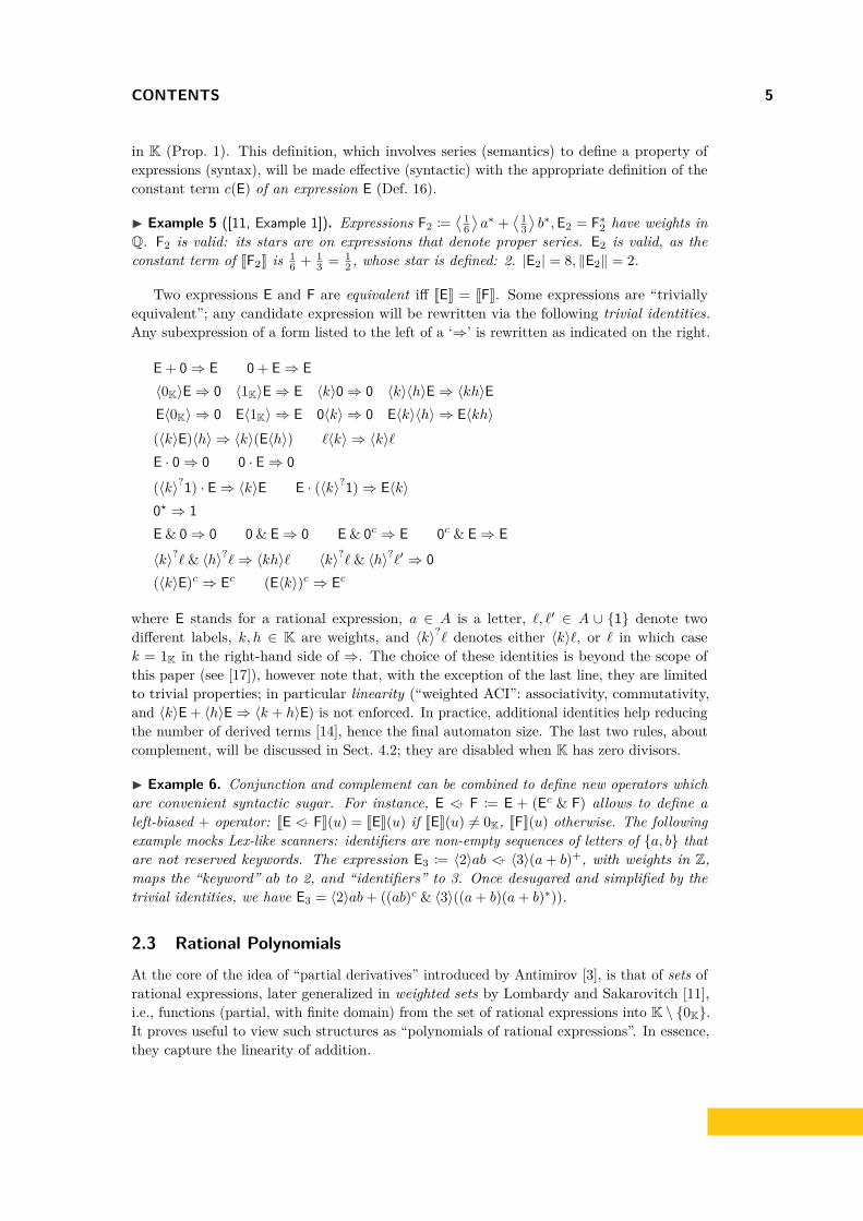
I Example 19 (Ex. 8 and 11 continued). Given d(E1), AE1 follows.d(E1) = X1 = 〈2〉 ⊕ a�

[〈2〉 � ce⊕ 〈4〉 � de

]⊕ b�

[〈6〉 � ce⊕ 〈3〉 � de

]

E1 = 〈5〉1+ 〈2〉ace+ 〈6〉bce+ 〈4〉ade+ 〈3〉bde〈5〉

ce

de

e 1

〈2〉a, 〈6〉b

〈4〉a, 〈3〉b

c

d

e

It is straightforward to extract an algorithm from Def. 18, using a work-list of states whoseoutgoing transitions to compute. This approach admits a natural lazy implementation: thewhole automaton is not computed at once, but rather, states and transitions are computedon-the-fly, on demand, for instance when evaluating a word.

I Theorem 20. Any (valid) expression E and its expansion-based derived-term automatonAE denote the same series, i.e., JAEK = JEK.

The smallness of the derived-term automaton for basic operators (|AE| ≤ ‖E‖ + 1 [11,Theorem 2]) no longer applies with extended operators. Let m and n be coprime integers,E := (am)∗&(an)∗ has width ‖E‖ = m+n; it is easy to see that |AE| = mn. It is also a classicalresult that the minimal (trim) automaton to recognize the language of Fn := (a+ b)∗a(a+ b)n

has 2n+1 states; so ‖Fcn‖ = 2n + 3, but |AFc

n| = 2n+1 + 1 (the additional state is the sink

state needed to get a complete deterministic automaton before complement). Actually, whencomplement is used on infinite semiring, it is not even guaranteed that the automaton isfinite (Sect. 4.2).

Sketch of proof of Theorem 20, see Appendix B. This result is proved as [11, Theorem 4]:it requires several lemmas whose proofs are simple, but long.

First define the derivation with respect to a word as the repetition of derivation withrespect to a letter, and prove that J∂uEK = u−1JEK.

Second, prove that the set of derivatives of an expression E with respect to words isgenerated by D(E), a set of expressions, called derived terms. The states of the derived-termautomaton are not any expressions, they are derived terms (and E itself), so the finiteness ofD(E) implies that of the automaton.

D(E) admits a simple inductive computation [11, Definition 3], to which we add:

D(E & F) := {Ei & Fj | ∀Ei ∈ D(E),∀Fj ∈ D(F)}D(Ec) := {(〈k1〉E1 + · · ·+ 〈kn〉En)c | ∀k1, . . . , kn ∈ K,∀E1, . . . ,En ∈ D(E)} (25)

If E features no complement, D(E) is trivially finite. Equation (25) is related to determinizedexpansions (Sect. 4.1): in essence it dubs (complements of) all potential derivatives of E intoderived-terms (comparable to going from Antimirov’s partial derivatives to Brzozowski’sderivatives). On infinite semirings, D(Ec) is infinite (more about this in Sect. 4.2). However,on finite semirings, such as B, it is finite, albeit potentially large.

Finally, prove that JAEK(u) = JEK(u) for all words u ∈ A∗. J

CONTENTS 11

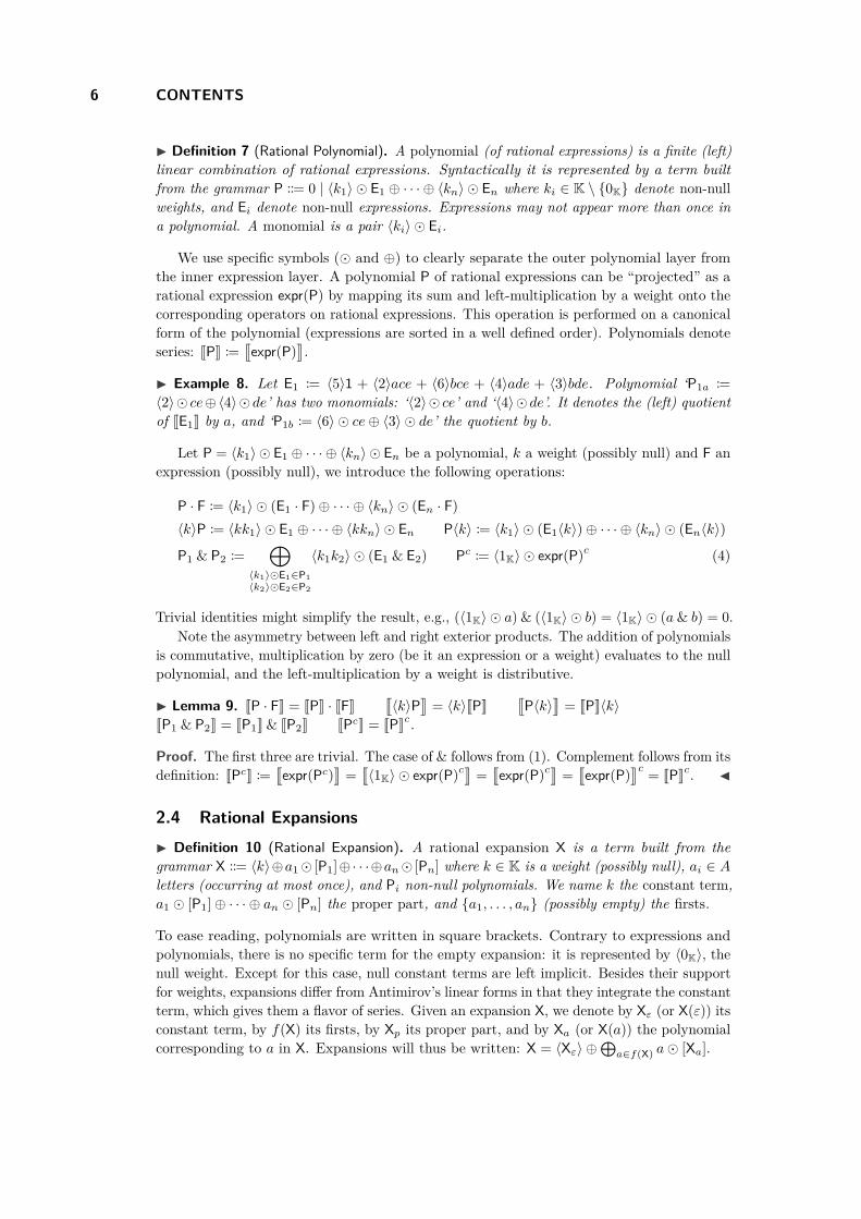
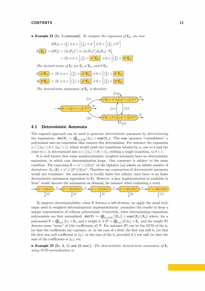
I Example 21 (Ex. 5 continued). To compute the expansion of E2, one has:

d(F2) = 〈 12 〉 ⊕ a�

[⟨ 16⟩� a∗

]⊕ b�

[⟨ 13⟩� b∗

]d( E2 ) = d(F∗2) =

⟨dε(F2)∗

⟩⊕⟨dε(F2)∗

⟩dp(F2) · F∗2

= 〈2〉 ⊕ a�[⟨ 1

3⟩� a∗ E2

]⊕ b�

[⟨ 23⟩� b∗ E2

]The derived terms of E2 are E2, a

∗E2, and b∗E2:

d( a∗E2 ) = 〈2〉 ⊕ a�[⟨ 4

3⟩� a∗ E2

]⊕ b�

[⟨ 23⟩� b∗ E2

]d( b∗E2 ) = 〈2〉 ⊕ a�

[⟨ 13⟩� a∗ E2

]⊕ b�

[⟨ 53⟩� b∗ E2

]The derived-term automaton of E2 is therefore:

E2 = (⟨16

⟩a∗ +

⟨13

⟩b∗)∗

〈2〉

a∗E2 = a∗ (⟨16

⟩a∗ +

⟨13

⟩b∗)∗

〈2〉

b∗E2 = b∗ (⟨16

⟩a∗ +

⟨13

⟩b∗)∗

〈2〉

〈 13 〉a

〈 23 〉b

〈 43 〉a

〈 23 〉b〈 13 〉a

〈 53 〉b4.1 Deterministic AutomataThe exposed approach can be used to generate deterministic automata by determinizingthe expansions: det(X) :=

⊕a∈f(X)〈1K〉 � expr(Xa). The expr operator “consolidates” a

polynomial into an expression that ensures this determinism. For instance the expansiona� [〈1K〉 � b⊕ 〈1K〉 � c], which would yield two transitions labeled by a, one to b and theother to c, is determinized into a� [〈1K〉 � (b+ c)], yielding a single transition, to b+ c.

It is well known that some nondeterministic weighted automata have no deterministicequivalent, in which case determinization loops. Our construct is subject to the samecondition. The expression E := a∗+ (〈2〉a)∗ on the alphabet {a} admits an infinite number ofderivatives: ∂an(E) = a∗⊕〈2n〉(〈2〉a)∗. Therefore our construction of deterministic automatawould not terminate: the automaton is locally finite but infinite (and there is no finitedeterministic automaton equivalent to E). However, a lazy implementation as available inVcsn1 would uncover the automaton on demand, for instance when evaluating a word.

a∗ + (〈2〉a)∗

〈2〉a∗ + 〈2〉(〈2〉a)∗

〈3〉a∗ + 〈4〉(〈2〉a)∗

〈5〉a∗ + 〈8〉(〈2〉a)∗

〈9〉a∗ + 〈16〉(〈2〉a)∗

〈17〉

a a a a

To improve determinizability, when K features a left-division, we apply the usual tech-nique used in weighted determinization implementations: normalize the results to keep aunique representative of colinear polynomials. Concretely, when determinizing expansions,polynomials are first normalized: det(X) :=

⊕a∈f(X)

⟨|Xa|

⟩� expr

(|Xa|\Xa

)where, for a

polynomial P =⊕

i∈I〈ki〉 � Ei, and a weight k, k\P :=⊕

i∈I

⟨k\ki

⟩� Ei, and the weight |P|

denotes some “norm” of (the coefficients of) P. For instance |P| can be the GCD of the ki

(so that the coefficients are coprime), or, in the case of a field, the first non null ki (so thatthe first non null coefficient is 1K), or the sum of the ki provided it’s not null (so that thesum of the coefficients is 1K), etc.

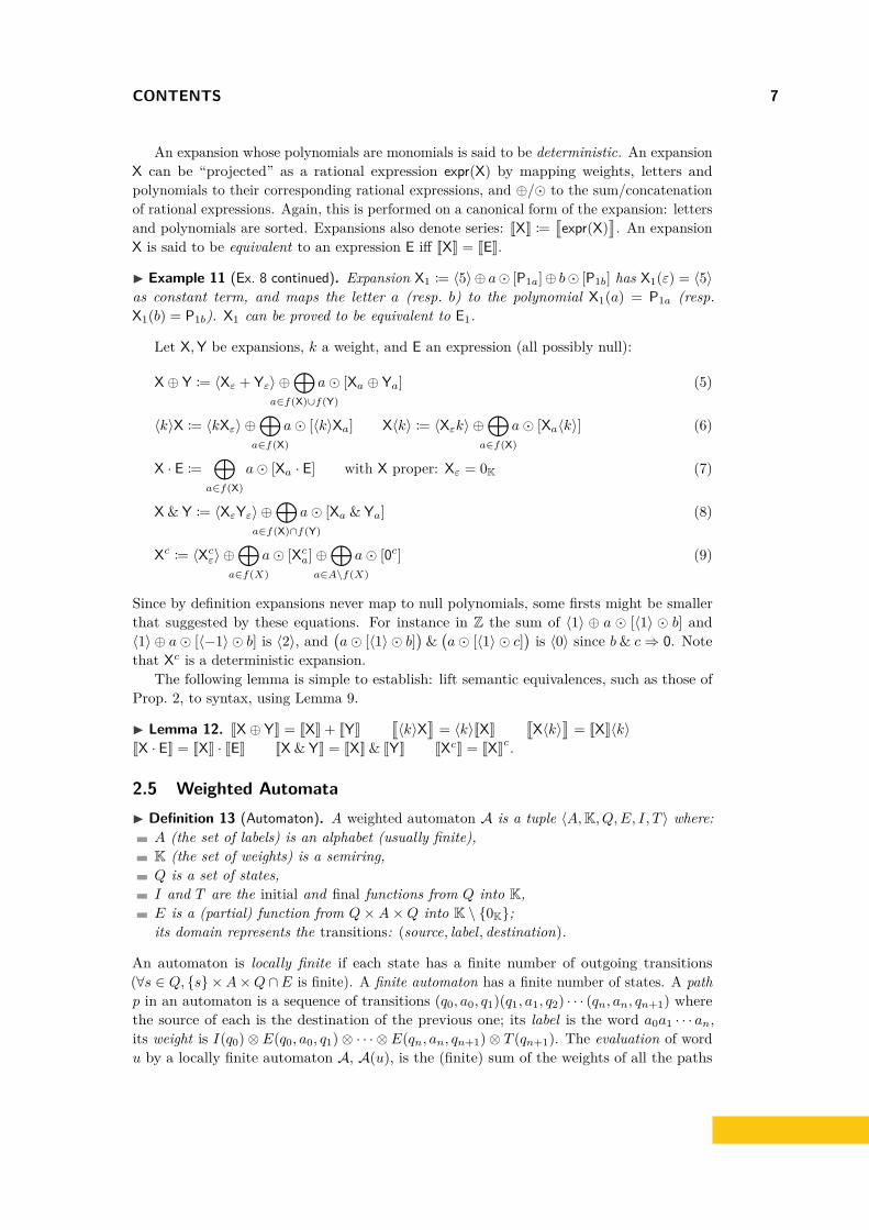
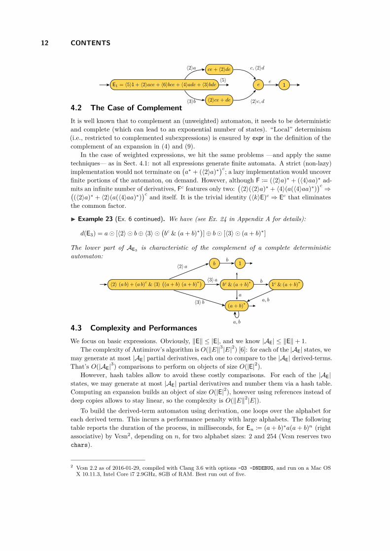
I Example 22 (Ex. 8, 11 and 19 cont.). The deterministic derived-term automaton of E1using GCD-normalization is:

12 CONTENTS

E1 = 〈5〉1+ 〈2〉ace+ 〈6〉bce+ 〈4〉ade+ 〈3〉bde〈5〉

ce+ 〈2〉de

〈2〉ce+ de

e 1

〈2〉a

〈3〉b

c, 〈2〉d

〈2〉c, d

e

4.2 The Case of ComplementIt is well known that to complement an (unweighted) automaton, it needs to be deterministicand complete (which can lead to an exponential number of states). “Local” determinism(i.e., restricted to complemented subexpressions) is ensured by expr in the definition of thecomplement of an expansion in (4) and (9).

In the case of weighted expressions, we hit the same problems —and apply the sametechniques— as in Sect. 4.1: not all expressions generate finite automata. A strict (non-lazy)implementation would not terminate on

(a∗ + (〈2〉a)∗

)c; a lazy implementation would uncoverfinite portions of the automaton, on demand. However, although F := (〈2〉a)∗ + (〈4〉aa)∗ ad-mits an infinite number of derivatives, Fc features only two:

(〈2〉(〈2〉a)∗ + 〈4〉(a(〈4〉aa)∗)

)c ⇒((〈2〉a)∗ + 〈2〉(a(〈4〉aa)∗)

)c and itself. It is the trivial identity (〈k〉E)c ⇒ Ec that eliminatesthe common factor.

I Example 23 (Ex. 6 continued). We have (see Ex. 24 in Appendix A for details):

d(E3) = a� [〈2〉 � b⊕ 〈3〉 �(bc & (a+ b)∗

)]⊕ b� [〈3〉 � (a+ b)∗]

The lower part of AE3 is characteristic of the complement of a complete deterministicautomaton:

〈2〉 (a b) + (a b)c& 〈3〉

((a+ b) (a+ b)

∗)

b

bc & (a+ b)∗ 1c & (a+ b)

∗

(a+ b)∗

1〈2〉 a

〈3〉 a

〈3〉 b

b

a

b

a, b

a, b

4.3 Complexity and PerformancesWe focus on basic expressions. Obviously, ‖E‖ ≤ |E|, and we know |AE| ≤ ‖E‖+ 1.

The complexity of Antimirov’s algorithm is O(‖E‖3|E|2) [6]: for each of the |AE| states, wemay generate at most |AE| partial derivatives, each one to compare to the |AE| derived-terms.That’s O(|AE|3) comparisons to perform on objects of size O(|E|2).

However, hash tables allow to avoid these costly comparisons. For each of the |AE|states, we may generate at most |AE| partial derivatives and number them via a hash table.Computing an expansion builds an object of size O(|E|2), however using references instead ofdeep copies allows to stay linear, so the complexity is O(‖E‖2|E|).

To build the derived-term automaton using derivation, one loops over the alphabet foreach derived term. This incurs a performance penalty with large alphabets. The followingtable reports the duration of the process, in milliseconds, for En := (a+ b)∗a(a+ b)n (rightassociative) by Vcsn2, depending on n, for two alphabet sizes: 2 and 254 (Vcsn reserves twochars).

2 Vcsn 2.2 as of 2016-01-29, compiled with Clang 3.6 with options -O3 -DNDEBUG, and run on a Mac OSX 10.11.3, Intel Core i7 2.9GHz, 8GB of RAM. Best run out of five.

CONTENTS 13

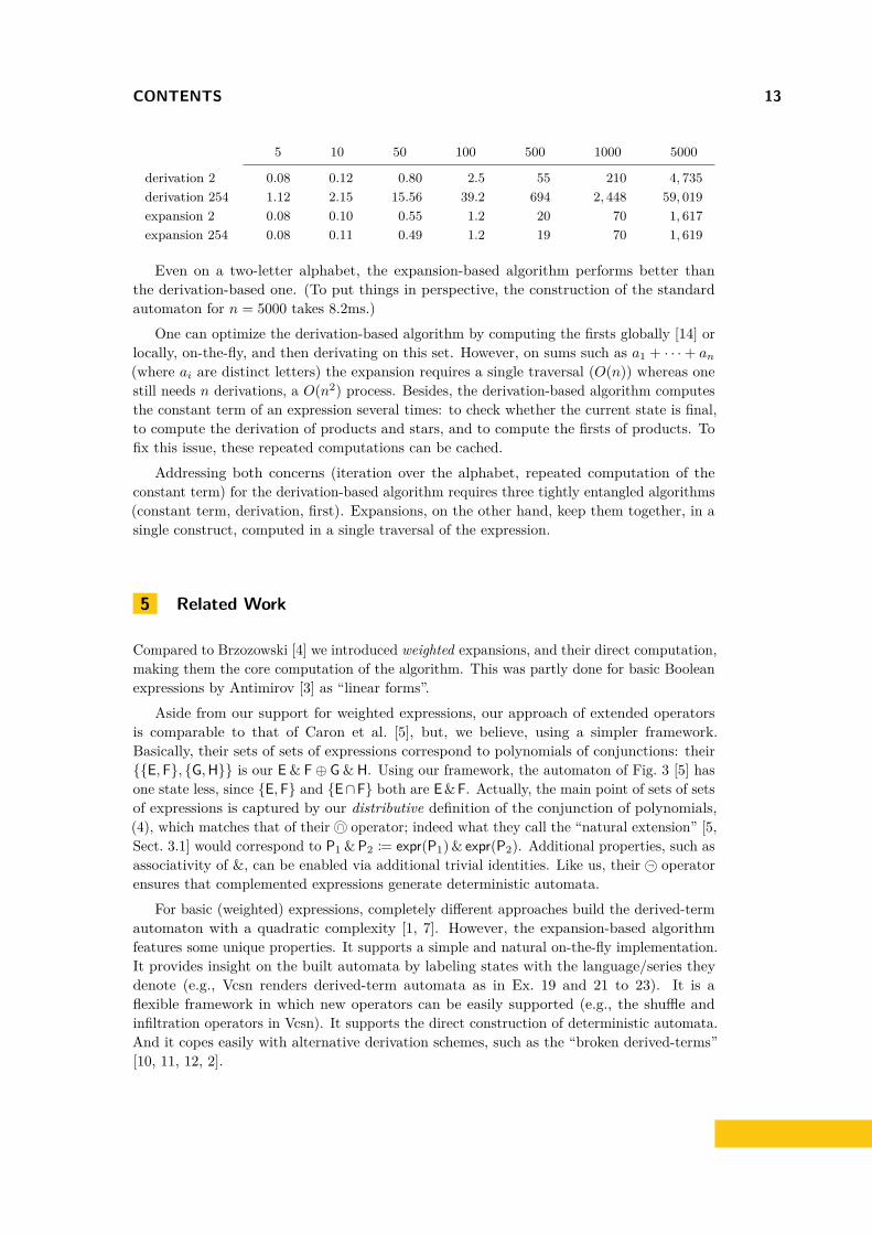
5 10 50 100 500 1000 5000

derivation 2 0.08 0.12 0.80 2.5 55 210 4, 735derivation 254 1.12 2.15 15.56 39.2 694 2, 448 59, 019expansion 2 0.08 0.10 0.55 1.2 20 70 1, 617expansion 254 0.08 0.11 0.49 1.2 19 70 1, 619

Even on a two-letter alphabet, the expansion-based algorithm performs better thanthe derivation-based one. (To put things in perspective, the construction of the standardautomaton for n = 5000 takes 8.2ms.)

One can optimize the derivation-based algorithm by computing the firsts globally [14] orlocally, on-the-fly, and then derivating on this set. However, on sums such as a1 + · · ·+ an

(where ai are distinct letters) the expansion requires a single traversal (O(n)) whereas onestill needs n derivations, a O(n2) process. Besides, the derivation-based algorithm computesthe constant term of an expression several times: to check whether the current state is final,to compute the derivation of products and stars, and to compute the firsts of products. Tofix this issue, these repeated computations can be cached.

Addressing both concerns (iteration over the alphabet, repeated computation of theconstant term) for the derivation-based algorithm requires three tightly entangled algorithms(constant term, derivation, first). Expansions, on the other hand, keep them together, in asingle construct, computed in a single traversal of the expression.

5 Related Work

Compared to Brzozowski [4] we introduced weighted expansions, and their direct computation,making them the core computation of the algorithm. This was partly done for basic Booleanexpressions by Antimirov [3] as “linear forms”.

Aside from our support for weighted expressions, our approach of extended operatorsis comparable to that of Caron et al. [5], but, we believe, using a simpler framework.Basically, their sets of sets of expressions correspond to polynomials of conjunctions: their{{E,F}, {G,H}} is our E & F⊕ G & H. Using our framework, the automaton of Fig. 3 [5] hasone state less, since {E,F} and {E∩F} both are E & F. Actually, the main point of sets of setsof expressions is captured by our distributive definition of the conjunction of polynomials,(4), which matches that of their ∩ operator; indeed what they call the “natural extension” [5,Sect. 3.1] would correspond to P1 & P2 := expr(P1) & expr(P2). Additional properties, such asassociativity of &, can be enabled via additional trivial identities. Like us, their ¬ operatorensures that complemented expressions generate deterministic automata.

For basic (weighted) expressions, completely different approaches build the derived-termautomaton with a quadratic complexity [1, 7]. However, the expansion-based algorithmfeatures some unique properties. It supports a simple and natural on-the-fly implementation.It provides insight on the built automata by labeling states with the language/series theydenote (e.g., Vcsn renders derived-term automata as in Ex. 19 and 21 to 23). It is aflexible framework in which new operators can be easily supported (e.g., the shuffle andinfiltration operators in Vcsn). It supports the direct construction of deterministic automata.And it copes easily with alternative derivation schemes, such as the “broken derived-terms”[10, 11, 12, 2].

14 REFERENCES

6 Conclusion

The construction of the derived-term automaton from a weighted rational expression is apowerful technique: states have a natural interpretation (they are identified by their future:the series they compute), extended rational expressions are easily supported, determinismcan be requested, and it even offers a natural lazy, on-the-fly, implementation to handleinfinite automata.

To build the derived-term automaton, we generalized Brzozowski’s expansions to weightedexpressions, and an inductive algorithm to compute the expansion of a rational expression.The formulas on which this algorithm is built reunite as a unique entity three facets thatwere kept separated in previous works: constant term, firsts, and derivatives. This resultsin a simpler set of equations, and an implementation whose complexity is independent ofthe size of the alphabet and even applies when it is infinite (e.g., when labels are strings,integers, etc.). Building the derived-term automaton using expansions is straightforward.Derivatives are only a technical tool to prove the correctness of the derived-terms. We havealso shown that using proper techniques, the complexity of the algorithm is much better thatpreviously reported.

The computation of expansions and derivations are implemented in Vcsn1, togetherwith their automaton construction procedures (possibly lazy, possibly deterministic). Ourimplementation actually prototypes support for additional operators on rational expressions(e.g., shuffle and infiltration). Our future work is focused on these operators.

Acknowledgments Interactions with A. Duret-Lutz, S. Lombardy, L. Saiu and J. Sakarovitchresulted in this work. Anonymous reviewers made very helpful comments.

References

1 C. Allauzen and M. Mohri. A unified construction of the Glushkov, follow, and Antimirovautomata. In MFCS, vol. 4162 of LNCS, pp. 110–121. Springer, 2006.

2 P.-Y. Angrand, S. Lombardy, and J. Sakarovitch. On the number of broken derived termsof a rational expression. Journal of Automata, Languages and Combinatorics, 15(1/2):27–51, 2010.

3 V. Antimirov. Partial derivatives of regular expressions and finite automaton constructions.TCS, 155(2):291–319, 1996.

4 J. A. Brzozowski. Derivatives of regular expressions. J. ACM, 11(4):481–494, 1964.5 P. Caron, J.-M. Champarnaud, and L. Mignot. Partial derivatives of an extended regular

expression. In LATA, vol. 6638 of LNCS, pp. 179–191. Springer, 2011.6 J.-M. Champarnaud and D. Ziadi. Canonical derivatives, partial derivatives and finite

automaton constructions. TCS, 289(1):137–163, 2002.7 J.-M. Champarnaud, F. Ouardi, and D. Ziadi. An efficient computation of the equation

K-automaton of a regular K-expression. In DLT, vol. 4588 of LNCS. Springer, 2007.8 A. Demaille, A. Duret-Lutz, S. Lombardy, and J. Sakarovitch. Implementation concepts

in Vaucanson 2. In CIAA’13, vol. 7982 of LNCS, pp. 122–133, July 2013. Springer.9 V. M. Glushkov. The abstract theory of automata. Russian Math. Surveys, 16:1–53,1961.

10 S. Lombardy and J. Sakarovitch. How expressions can code for automata. In LATIN, pp.242–251, 2004.

REFERENCES 15

11 S. Lombardy and J. Sakarovitch. Derivatives of rational expressions with multiplicity.TCS, 332(1-3):141–177, 2005.

12 S. Lombardy and J. Sakarovitch. Corrigendum to our paper: How expressions can codefor automata. RAIRO — Theoretical Informatics and Applications, 44(3):339–361, 2010.

13 R. McNaughton and H. Yamada. Regular expressions and state graphs for automata.IEEE Transactions on Electronic Computers, 9:39–47, 1960.

14 S. Owens, J. Reppy, and A. Turon. Regular-expression derivatives re-examined. J. Funct.Program., 19(2):173–190, Mar. 2009.

15 J. J. M. M. Rutten. Automata, power series, and coinduction: Taking input derivativesseriously. In Automata, Languages and Programming, 26th International Colloquium,ICALP’99, Prague, Czech Republic, July 11-15, 1999, Proceedings, vol. 1644 of LNCS,pp. 645–654. Springer, 1999.

16 J. J. M. M. Rutten. Behavioural differential equations: a coinductive calculus of streams,automata, and power series. TCS, 308(1-3):1–53, 2003.

17 J. Sakarovitch. Elements of Automata Theory. Cambridge University Press, 2009.Corrected English translation of Éléments de théorie des automates, Vuibert, 2003.

A Appendix

Proof of Lemma 12. Most operators are trivial, we focus here on the extended operators.

JX & YK =

u

v〈XεYε〉 ⊕⊕

a∈f(X)∩f(Y)

a� [Xa & Ya]

}

~ by definition, (8)

= XεYε +∑

a∈f(X)∩f(Y)

a · JXa & YaK by definition of expr

= XεYε +∑

a∈f(X)∩f(Y)

a ·(JXaK & JYaK

)by Lemma 9

=

Xε +∑

a∈f(X)

a · JXaK

&

Yε +∑

a∈f(Y)

a · JYaK

by (2)

=

u

v〈Xε〉 ⊕⊕

a∈f(X)

a · [Xa]

}

~ &

u

v〈Yε〉 ⊕⊕

a∈f(Y)

a · [Ya]

}

~

= JXK & JYK

JXcK =

u

v〈Xcε〉 ⊕

⊕a∈f(X)

a� [Xca]⊕

⊕a∈A\f(X)

a� [0c]

}

~ by definition, (9)

= Xcε +

∑a∈f(X)

a · JXcaK +

∑a∈A\f(X)

a · J0cK

= Xcε +

∑a∈f(X)

a · JXaKc +∑

a∈A\f(X)

a · J0Kc by Lemma 9

=

Xε +∑

a∈f(X)

a · JXaK

c

by (3)

16 REFERENCES

= JXKc J

I Example 24 (Ex. 23 detailed). We have:

d((ab)c

)= d(ab)c =

(〈a〉 � [b]

)c = 〈1K〉 ⊕ a� [bc]⊕ b� [0c]

d(〈3〉(a+ b)(a+ b)∗

)= 〈3〉d

((a+ b)(a+ b)∗

)= 〈3〉dp(a+ b) · (a+ b)∗ ⊕

⟨dε(a+ b)

⟩d((a+ b)∗

)= 〈3〉

(a� [〈1〉 � 1]⊕ b� [〈1〉 � 1]

)· (a+ b)∗ ⊕ 〈0K〉d

((a+ b)∗

)= 〈3〉

(a� [〈1〉 � (a+ b)∗]⊕ b� [〈1〉 � (a+ b)∗]

)= a� [〈3〉 � (a+ b)∗]⊕ b� [〈3〉 � (a+ b)∗]

therefore:

X := d((ab)c

)& d(〈3〉(a+ b)(a+ b)∗

)=(〈1K〉 ⊕ a� [bc]⊕ b� [0c]

)&(〈a〉 � [〈3〉 � (a+ b)∗]⊕ 〈b〉 � [〈3〉 � (a+ b)∗]

)= a� [〈3〉 �

(bc & (a+ b)∗

)]⊕ b� [〈3〉 �

(0c & (a+ b)∗

)]

= a� [〈3〉 �(bc & (a+ b)∗

)]⊕ b� [〈3〉 � (a+ b)∗]

and finally

d(E3) = d(〈2〉ab+ (ab)c & 〈3〉(a+ b)(a+ b)∗

)= d(〈2〉ab

)⊕ d((ab)c & 〈3〉(a+ b)(a+ b)∗

)= a� [〈2〉 � b]⊕

X︷ ︸︸ ︷(d((ab)c

)& d(〈3〉(a+ b)(a+ b)∗

))= a� [〈2〉 � b]⊕ a� [〈3〉 �

(bc & (a+ b)∗

)]⊕ b� [〈3〉 � (a+ b)∗]

= a� [〈2〉 � b⊕ 〈3〉 �(bc & (a+ b)∗

)]⊕ b� [〈3〉 � (a+ b)∗]

B Appendix: Proof of Theorem 20

Proving this theorem requires several auxiliary results. None of them is needed in animplementation: Def. 14 is all that is needed to build the derived-term automaton.

The path, paved by Lombardy and Sakarovitch [11], is as follows. First, define derivationwith respect to a word, and show that it is a syntactic “implementation” of left-quotientof a series by a word (Appendix B.1). Then define (syntactically) the set of derived terms,and show that they generate all the word derivatives (Appendix B.2). Finally show thatcomputations in the derived-term automaton correspond to computing the left-quotient ofthe denoted series (Appendix B.3).

This is also the path followed by the rather terse proof of Caron et al. [5, Proposition 4],but filling the gaps.

B.1 Derivation by WordsI Definition 25 (Derivation of a Polynomial). ∂a ⊕i∈I 〈ki〉 � Ei := ⊕i∈I〈ki〉 � ∂aEi

I Lemma 26.∂a(P & Q) = ∂aP & ∂aQ (26)∂aexpr(P) = expr(∂aP) (27)

∂a(Pc) = (∂aP)c (28)

REFERENCES 17

Proof. Let P :=⊕

i∈I〈ki〉 � Ei,Q :=⊕

j∈J

⟨hj

⟩� Fj .

∂a(P & Q) = ∂a

⊕i∈I,j∈J

⟨kihj

⟩� Ei & Fj

by def. of polynomial conjunction

=⊕

i∈I,j∈J

⟨kihj

⟩� ∂a

(Ei & Fj

)=

⊕i∈I,j∈J

⟨kihj

⟩�(∂aEi & ∂aFj

)by (23)

= ∂aP & ∂aQ by def. of polynomial conjunction

∂aexpr(P) = ∂aexpr

⊕i∈I

〈ki〉 � Ei

= ∂a

∑i∈I

〈ki〉Ei

=∑i∈I

〈ki〉∂aEi

= expr

⊕i∈I

〈ki〉 � ∂aEi

= expr(∂aP)

∂a(Pc) = ∂a

(expr(P)c) by def. of polynomial complement

=(∂a

(expr(P)

))c

by (24)

=(expr(∂aP)

)c by (27)= (∂aP)c by def. of polynomial complement J

Derivation wrt a single-letter word is defined as the derivation wrt that letter. Derivationwrt to a longer word is the result of repeated derivations wrt letters.

I Definition 27 (Derivation wrt a Word). ∀a ∈ A, u ∈ A+, ∂uaE := ∂a∂uE.

I Lemma 28. ∂uvE = ∂v∂uE

Explicit formulas exist for derivation with respect to a word.

I Lemma 29 (Direct Computations of Derivation wrt a Word).∂u(E + F) = ∂uE⊕ ∂uF, (29)∂u(〈k〉E) = 〈k〉(∂uE), (30)∂u(E〈k〉) = (∂uE)〈k〉, (31)

∂u(E · F) = (∂uE) · F⊕

⊕f=gh

g∈A∗,h∈A+

c(∂gE)∂hF

(32)

18 REFERENCES

∂uE∗ =⊕

f=g1g2···gn

g1,...,gn∈A+

⟨ ∏i∈[n−1]

c(E)∗c(∂giE)

c(E)∗⟩∂gn

E · E∗ (33)

∂u(E & F) = ∂uE & ∂uF, (34)∂uEc = (∂uE)c (35)

Proof. The proof is the same as that of [11, Prop. 3], with additional cases for conjunctionand complement.

For conjunction:

∂ua(E & F) = ∂a∂u(E & F)= ∂a(∂uE & ∂uF) by induction hypothesis= ∂a∂uE & ∂a∂uF by (26)= ∂uaE & ∂uaF

For complement:

∂ua(Ec) = ∂a∂u(Ec)= ∂a(∂uE)c by induction hypothesis=(∂a(∂uE)

)c by (28)= (∂uaE)c J

The following lemma makes explicit the connection between the (syntactic) derivation,and the semantics of an expression.

I Lemma 30 ([11, Prop. 4]). ∀u ∈ A+, JEK(u) = c(∂uE).

Proof. For conjunction:

JE & FK(u) =(JEK & JFK

)(u) by definition

= JEK(u) · JFK(u) by definition= c(∂uE) · c(∂uF) by induction hypothesis= c(∂uE & ∂uF) by (23)= c(∂u(E & F)) by (34)

For complement:

JEcK(u) = JEKc(u) by definition= (JEK(u))c by definition= (c(∂uE))c by induction hypothesis= c((∂uE)c) by (24)= c(∂u(Ec)) by (35) J

The previous lemma allows to show the connection between the (syntactic) derivation,and the (semantical) left-quotient of a series.

I Theorem 31 ([11, Theorem 1]). ∀u ∈ A+, J∂uEK = u−1JEK.

REFERENCES 19

Proof. For any word v ∈ A+,

J∂uEK(v) = c(∂v∂uE) by Lemma 30= c(∂uvE) by Lemma 28= JEK(uv) by Lemma 30= (u−1JEK)(v) by definition of left-quotient J

B.2 Derived TermsI Definition 32 (Derived Terms). Given an expression E, its derived terms is the set D(E)defined as follows:

D(0) := ∅D(1) := ∅D(a) := {1} ∀a ∈ A

D(E + F) := D(E) ∪D(F)D(〈k〉E) := D(E) ∀k ∈ KD(E〈k〉) := {Ei〈k〉 | Ei ∈ D(E)} ∀k ∈ KD(E · F) := {Ei · F | Ei ∈ D(E)} ∪D(F)D(E∗) := {Ei · E∗ | Ei ∈ D(E)}

D(E & F) := {Ei & Fj | ∀Ei ∈ D(E),∀Fj ∈ D(F)}D(Ec) := {(〈k1〉E1 + · · ·+ 〈kn〉En)c | ∀k1, . . . , kn ∈ K,∀E1, . . . ,En ∈ D(E)}

where in the last equation, the Ei are sorted. Besides, depending on the features of K, thecoefficients may be normalized so that colinear combinations are represented only once. Forinstance if K has no zero divisor, one may divide by the GCD of the ki (so that the ki

are coprime), or, in the case of a field, by the first non null ki (so that the first non nullcoefficient is 1K), or by the sum of the ki provided it’s not null (so that the sum of thecoefficients is 1K), etc.

I Theorem 33. If K is finite, or if E has no complement, then D(E) is finite.

Proof. This is a direct consequence from Def. 32: finiteness propagates during the induction.The only danger is the case of complement, whose finiteness ensues from a very crude criterion:there exists a finite number of combinations. J

We prove that the set of derived terms is closed by derivation. The insightful reader cansee automata dawning: the derived terms are the states, and the coefficients are the weightsof the transitions.

I Lemma 34. We denote {1, . . . , n} by [n].Let E be an expression, D(E) = {Ei | i ∈ [n]} be its derived terms. There exists n

coefficients (k(a)i )i∈[n] and n2 coefficients (k(a)

i,j )i,j∈[n] such that

∂aE =⊕i∈[n]

⟨k

(a)i

⟩Ei ∂aEi =

⊕i′∈[n]

⟨k

(a)i,i′

⟩Ei′

Proof. We follow [11, proof of Theorem 2], to which we add the following cases. We note:

D(F) = {Fj | j ∈ [m]} ∂aF =⊕

j∈[m]

⟨h

(a)j

⟩Fj ∂aFj =

⊕j′∈[m]

⟨h

(a)j,j′

⟩Fj′

20 REFERENCES

Consider E & F:

∂a(E & F) = ∂aE & ∂aF

=

⊕i∈[n]

⟨k

(a)i

⟩Ei

&

⊕j∈[m]

⟨h

(a)j

⟩Fj

=

⊕i∈[n],j∈[m]

⟨k

(a)i h

(a)j

⟩(Ei & Fj

)which is indeed a linear combination of derived terms of E & F, since D(E & F) = {Ei & Fj |∀Ei ∈ D(E),∀Fj ∈ D(F)} by definition Def. 32.

Likewise,

∂a(Ei & Fj) = ∂aEi & ∂aFj

=

⊕i′∈[n]

⟨k

(a)i,i′

⟩Ei′

&

⊕j′∈[m]

⟨h

(a)j,j′

⟩Fj′

=

⊕i′∈[n],j′∈[m]

⟨k

(a)i,i′h

(a)j,j′

⟩(Ei′ & Fj′

)is a linear combination of elements of D(E & F).

Consider Ec:

∂a(Ec) = (∂aE)c

=

⊕i∈[n]

⟨k

(a)i

⟩Ei

c

=

expr

⊕i∈[n]

⟨k

(a)i

⟩Ei

c

=

∑i∈[n]

⟨k

(a)i

⟩Ei

c

which is a member of D(Ec). Note in this case, we expect the Ei to be sorted in the sameorder as the one used by expr.

Besides:

∂a

∑

i∈[n]

⟨k

(a)i

⟩Ei

c =

∂a

∑i∈[n]

⟨k

(a)i

⟩Ei

c

=

⊕i∈[n]

⟨k

(a)i

⟩∂aEi

c

=

⊕i∈[n]

⟨k

(a)i

⟩⊕i′∈[n]

⟨k

(a)i,i′

⟩Ei′

c

=

⊕i,i′∈[n]

⟨k

(a)i k

(a)i,i′

⟩Ei′

c

REFERENCES 21

=

∑i,i′∈[n]

⟨k

(a)i k

(a)i,i′

⟩Ei′

c

which is a member of D(Ec). J

The following result, similar to [11, Theorem 3], shows that any word derivative of anexpression is a linear combination of its derived terms.

I Theorem 35. Let E be an expression, D(E) = {Ei | i ∈ [n]} be its derived terms, andu ∈ A+ any word. There exist coefficients (k(u)

i )i∈[n] in K such that:

∂uE =⊕i∈[n]

⟨k

(u)i

⟩Ei

Proof. The result is proved by induction.The base case is established by Lemma 34.

∂uaE = ∂a∂uE

= ∂a

⊕i∈[n]

⟨k

(u)i

⟩Ei

by induction hypothesis

=⊕i∈[n]

⟨k

(u)i

⟩∂aEi

=⊕i∈[n]

⟨k

(u)i

⟩⊕j∈[n]

⟨k

(a)i,j

⟩Ej

by Lemma 34

=⊕j∈[n]

⊕i∈[n]

⟨k

(u)i k

(a)i,j

⟩Ej

=⊕j∈[n]

⟨∑i∈[n]

k(u)i k

(a)i,j

⟩Ej

i.e.,

k(ua)j =

∑i∈[n]

k(u)i k

(a)i,j (36)

J

B.3 Derived-term AutomatonIn order to prove the final result, we express automata in a different way [11, Sect. 5].

I Definition 36 (Representations of a Finite Weighted Automaton). The matrix representationof a (finite weighted) automaton is the sextuplet 〈A,K, E,Q,E, I, T 〉 where:

A is an alphabetK (the set of weights) is a semiring,Q is a finite set of states,I (resp. T ) is a row (resp. column) vector of dimension Q with entries in K,E is a square matrix whose entries are linear combinations of letters of A with coefficientsin K.

22 REFERENCES

The K-representation of an automaton is the triple 〈I, ζ, T 〉 where ζ is a morphism fromA to KQ×Q such that E =

∑a∈A ζ(a)a.

One can then prove that, for every word u ∈ A∗:

JAK(u) = (I · E∗ · T )(u) = (I · E|u| · T )(u) = I · ζ(u) · T

Put together, the definition of derivation and constant terms (Def. 16), their connectionwith expansions (Prop. 17), the definition of AE, the expansion-based derived-term automatonof E (Def. 18), and finally Lemma 34, show that AE admits the following K-representation:

IEi=

1K if Ei = E0K otherwise

ζ(a)i,j = k(a)i,j TEi

= c(Ei)

where the coefficients k(a)i,j were defined in Lemma 34. The Ei are the derived-terms of E, to

which we add E0 := E if E 6∈ D(E), in which case k(a)i,0 := 0K, and k(a)

0,i := k(a)i for all i > 0.

We prove by induction that:

∀u ∈ A+,∀i ∈ [n], (I · ζ(u))i = k(u)i (37)

Proof. The base case:

(I · ζ(a))i =∑

j

(Ij · ζ(a)j,i

= 1K · ζ(a)0,i by definition of I

= k(a)0,i by definition of ζ

= k(a)i by definition of k(a)

i,j

Then the induction:

(I · ζ(ua))i = (I · (ζ(u) · ζ(a)))i

= ((I · ζ(u)) · ζ(a))i

=∑

j

(I · ζ(u))j · ζ(a)j,i)

=∑

j

(k(u)j · ζ(a)j)i by induction hypothesis

=∑

j

(k(u)j · k(a)

j,i ) by definition of ζ

= k(ua)i by (36) J

We can now finally prove that JAEK = JEK. Let u ∈ A+:

JAEK(u) = (I · ζ(u) · T )

=∑

i

(I · ζ(u))i · Ti

=∑

i

k(u)i · Ti by (37)

=∑

i

k(u)i · c(Ei) by definition of T

REFERENCES 23

= c

⊕i

⟨k

(u)i

⟩Ei

= c(∂uE) by Theorem 35= JEK(u) by Theorem 31

The case of the empty word follows from the definition of I and T : JAEK(ε) =∑

i(Ii.Ti) =1K · T0 = c(E).