Derivatives for Time-Spectral Computational Fluid Dynamicsusing an Automatic Differentiation Adjoint

Charles A. Mader∗

University of Toronto Institute for Aerospace StudiesToronto, Ontario, Canada

Joaquim R.R.A. Martins†

Department of Aerospace Engineering, University of MichiganAnn Arbor, Michigan

In computational fluid dynamics, for problems with periodic flow solutions, the computational costof spectral methods is significantly lower than that of full, unsteady computations. As is the casefor regular steady-flow problems, there are various interesting periodic problems, such as those in-volving helicopter rotor blades, wind turbines, or oscillating wings, that can be analyzed with spec-tral methods. When conducting gradient-based numerical optimization for these types of problems,efficient sensitivity analysis is essential. We develop an accurate and efficient sensitivity analysisfor time-spectral computational fluid dynamics. By combining the cost advantage of the spectral-solution methodology with an efficient gradient computation, we can significantly reduce the totalcost of optimizing periodic unsteady problems. The efficient gradient computation takes the formof an automatic differentiation discrete adjoint method, which combines the efficiency of an adjointmethod with the accuracy and rapid implementation of automatic differentiation. To demonstratethe method, we compute sensitivities for an oscillating ONERA M6 wing. The sensitivities are shownto be accurate to 8–12 digits, and the computational cost of the adjoint computations is shown to scalewell up to problems of more than 41 million state variables.

Nomenclatureα angle of attackCL average lift coefficientCD average drag coefficientCm average pitch moment coefficientDt spectral derivative operatoret total energyfi flux term (Section III), function (Section V)h step sizeI function of interestk frequency indexl time instance indexM Freestream Mach numbern time instance indexN number of spectral time intervalsNcells number of cells in meshNI number of functions of interestNx number of design variablesNζ number of states per cellNζT total number of statesp pressuret time (Sections III and IV), intermediate variables (Section V)T time period of periodic flow problemu flow velocity with respect to fixed frame

∗Ph.D Candidate, AIAA Student Member†Associate Professor, AIAA Senior Member

1 of 20

American Institute of Aeronautics and Astronautics (In press-AIAA Journal)

v flow velocity with respect to moving gridV volumew velocity of moving gridx time interval (Section III), design variables (Section IV)y coordinate directionδi elements of identity matrixψ adjoint vectorρ densityζ flow statesR steady-state flow residualsRT S time-spectral flow residuals

I. IntroductionFor cost-effective gradient-based optimization, both efficient function analysis and efficient sensitivity analysis are

needed. In this work, we demonstrate the application of the ADjoint method, an efficient sensitivity analysis method,to a time-spectral computational fluid dynamics solver; the latter is an efficient method for solving periodic unsteadyflow problems. As the background section will show, significant progress has been made in both the developmentof adjoint techniques and the solution of periodic unsteady problems. Building on this previous work, we apply theaccurate and efficient ADjoint technique to the time-spectral equations, producing sensitivities that are demonstrablymore accurate than those of previous time-spectral adjoint implementations. Further, we demonstrate the scaling ofthe method to cases of up to 41 million flow states, showing that it is valid and useful for practical problem sizes. Asummary of related work is presented in the background section, and the implementation of our method is discussedin the implementation section.

II. BackgroundThe adjoint method for sensitivity analysis is now commonly used in aerodynamic shape optimization. The ap-

plication of the adjoint method to fluid dynamics was first developed by Pironneau [1], who demonstrated how tominimize the drag over bodies immersed in laminar viscous flows. Jameson [2] applied the adjoint method to theEuler-based aerodynamic shape optimization of airfoils and wings. Since these seminal contributions, the method hasbeen applied to the optimization of airfoils including viscous effects [3, 4, 5, 6], laminar-turbulent transition predic-tion [7], and to multi-point airfoil optimization problems [6, 8]. The adjoint method has also been extended to threedimensions and used to optimize wings for inviscid flows [9, 10] and viscous flows [11, 12] as well as for multi-pointwing problems [13] and full-wing body configurations [14, 15]. The applications of the method go beyond shapeoptimization with strictly aerodynamic considerations: it has been applied to sonic-boom reduction [16], hypersonicflows including magneto-hydrodynamic effects [17, 18], and coupled aerostructural design [19, 20]. In each case, theadjoint method enabled efficient design optimization with large numbers of variables.

While the adjoint method is relatively common in steady-state optimizations—at least in the research community—it is still relatively uncommon in time-dependent problems. The adjoint solution of two-dimensional time-dependentproblems was demonstrated by Nadarajah and Jameson [21], Mani and Mavriplis [22], Rumpfkeil and Zingg [23],and Wang et al. [24]. A three-dimensional adjoint solution was developed by Mavriplis [25]. These methods area significant improvement over finite-difference sensitivity methods, but they still have a high computational cost.The unsteady adjoint computation requires a reverse integration in time from the final solution back to the initialcondition [22, 21]. Thus, a time-dependent adjoint requires the full forward solution of the unsteady problem, storingthe flow states for each time step along the way, followed by a reverse sweep of the solution process to find the adjointsolution. While this process is more efficient than computing a full unsteady solution for every design variable inthe problem, it is expensive. Various methods for reducing the computational requirements have been suggested, forexample writing the solution history to disk rather than storing the solution in memory [22], evaluating only a periodicportion of the time history for the adjoint problem [21, 23], or using checkpointing algorithms in combination withautomatic differentiation [26]. However, even with these additions, the computational cost of the full unsteady adjointmethod is significant.

Recently, the use of spectral methods to discretize the time-domain portion of periodic CFD problems has gainedpopularity. These methods exploit the periodic nature of the problem by expressing the states of the system as a Fourierseries in time. The entire periodic solution can then be recovered from a small number of representative state instances

2 of 20

American Institute of Aeronautics and Astronautics (In press-AIAA Journal)

spanning the time period, or frequency spectrum, of the solution. These state instances can then be solved for directly,eliminating the need to iterate through the starting transients typical of unsteady CFD solutions.

In this context, spectral-method computations can be performed in either the time domain, the frequency domain,or a combination of the two. In the time domain, the state instances represent discrete snapshots of the solution in time,while in the frequency domain, the state instances represent distinct frequencies present in the solution. In each case,the spectral solution is capable of representing a fundamental frequency as well as a number of higher harmonics. Thenumber of resolved harmonics is related to the number of time or frequency instances present in the solution.

Early work on time nonlinear spectral solution techniques was conducted by Hall et al. [27], who derived a spec-tral formulation for the two-dimensional Navier–Stokes equations. This derivation was conducted in the frequencydomain, but to facilitate the computation they transformed the flow equations back to the time domain. This alloweda typical time-domain residual formulation to be used for the computation of the solution in each of the spectral in-stances. This residual was augmented by a spectral term that coupled the various solution instances. The residualswere computed in the time domain, but both the spectral operator and the boundary conditions were applied in thefrequency domain, yielding a mixed time-domain/frequency-domain approach. In an extension of this work, Ekici andHall [28] applied this technique, known as the harmonic balance technique, to multistage turbomachinery applicationswhere a variety of frequencies may be present.

The time-spectral method introduced by Gopinath and Jameson [29, 30] is similar to the harmonic balance methodof Hall et al. [27]. However, the time-spectral method is derived completely in the time domain. This yields a purelyreal spectral operator, and allows for the use of the time-domain residual operator in its original form, includingthe boundary conditions. This is particularly advantageous in the context of the present work, because it allowsus to check the newly developed time-spectral ADjoint sensitivities against those computed using the complex-stepmethod [31, 32, 33, 34]. This verification is not possible for codes that use frequency-domain analysis, since they usecomplex arithmetic in the solution process.

Another nonlinear spectral solution technique is the nonlinear frequency domain (NLFD) method developed byMcMullen et al. [35, 36, 37]. In this technique, the solution process takes place primarily in the frequency domain.The states of the system are stored as frequency-domain Fourier coefficients, and the solution steps are generated fromthe frequency-domain residual and spectral operator. To simplify the implementation, the residual is evaluated in thetime domain, where the states are transformed from the frequency domain to the time domain. Then, the residual istransformed from the time domain to the frequency domain using fast Fourier transform (FFT) techniques.

The time-spectral CFD method reduces the computational cost of a periodic unsteady flow solution relative to a fullunsteady flow solution for periodic problems. Similarly, the time-spectral adjoint method can dramatically reduce thecomputational cost of an optimization problem that involves a periodic unsteady problem. Just as the spectral solutiontechnique modifies a single unsteady CFD problem into a set of coupled steady CFD problems, the time-spectraladjoint technique converts a full unsteady adjoint problem into a single large steady adjoint problem. Coupling thiswith the efficient solution of large sparse linear systems provided by modern software packages, such as PETSc [38],allows us to rapidly implement an adjoint technique for periodic unsteady problems.

Adjoint methods have been developed for each of the spectral methods mentioned above. Thomas et al. [39] de-veloped an adjoint for the two-dimensional viscous harmonic balance equations. They used a combination of forward-and reverse-mode automatic differentiation (AD) to generate the terms necessary for the adjoint. They computedmesh sensitivities for an airfoil and verified their implementation using finite-difference sensitivities as the bench-mark. Nadarajah and Jameson [40] developed an adjoint implementation for the NLFD equations. They used analytictechniques to derive a discrete adjoint operator for the NLFD solver. The resulting technique was used to optimize anoscillating transonic wing. Finally, Choi et al. [41] developed an adjoint implementation for the time-spectral equa-tions. They used a manually coded adjoint method and a time-spectral flow solver to calculate the gradients requiredfor a helicopter rotor-blade optimization. The method improved the blades, but the adjoint implementation did notachieve the full numerical accuracy that is theoretically possible with a discrete adjoint method. This limited accuracywas the result of approximations made in the differentiation of the functions related to the spectral radius and artificialdissipation.

We use the automatic differentiation adjoint (ADjoint) approach of Mader et al. [42] to generate the discreteadjoint operator. Similarly to the work by Thomas et al. [39], this approach combines AD and adjoint methods togenerate accurate and efficient sensitivities. The characteristics of the adjoint method ensure an efficient method forcomputing the sensitivities of a small number of output functions of interest with respect to a large number of designvariables. The use of AD ensures that the partial derivatives used in the adjoint formulation are accurate and reducesthe time required to compute those derivatives. We extend our method to a three-dimensional time-spectral CFD solver,providing a detailed overview of the implementation, and demonstrate the resulting code on large-scale problems withup to 41 million flow states. Further, we conclusively demonstrate the accuracy of the method by comparing the

3 of 20

American Institute of Aeronautics and Astronautics (In press-AIAA Journal)

derivatives computed to those computed with the complex-step method. In the following sections, we introduce eachof the components—the time-spectral flow solver, the adjoint method, and automatic differentiation—and then discusshow these components are used in the implementation of a time-spectral ADjoint. We then demonstrate the accuracyand efficiency of the method on an oscillating-wing test case.

III. Time-Spectral Computational Fluid DynamicsWe first review the time-spectral flow solver and its relation to the steady flow solver. The particular spectral

method that we use, the time-spectral method, was derived by Gopinath et al. [29, 43]. As discussed in the Introduction,this method is one of a class of solution techniques based on representing the time derivative operator in the flowequations as a Fourier series. Expressing the time derivative operator in this fashion allows for a significant reductionin the number of time snapshots needed to model the flow, thereby reducing the computational cost of the solution. Inparticular, this method focuses on expressing the time derivative strictly in the time domain, which eliminates the needto use complex numbers and FFTs in the solution process. The details of this method and the resulting time derivativeoperator can be found in Gopinath [30]. The specific implementation of the time-spectral method used here is thatof the SUmb flow solver [44]. SUmb is a cell-centered multiblock solver for the Reynolds-averaged Navier–Stokesequations—steady, unsteady, and time-spectral—and it has options for a variety of turbulence models with one, two,and four equations. The details of the flow equations in this context are given below.

To put the derivation of the time-spectral adjoint sensitivity equations in context, we provide a basic derivation ofthe time-spectral flow equations. We start by writing the governing equations for unsteady flow,

V∂ζ

∂t+∂fi∂yi

= 0, (1)

where yi are the coordinates in the ith direction. We assume a nondeforming mesh, so the cell volume, V , can bemoved outside the time derivative.

Because we are simulating periodic problems, grid motion needs to be accounted for, so the velocity of the grid,w, is included in the flux term. A more detailed discussion of the formulation used in our flow solver can be found inMader and Martins [45]. Based on this formulation, the inviscid flow states and fluxes for each cell are

ζ =

ρρu1ρu2ρu3ρet

, fi =

ρui − ρwi

ρuiu1 − ρwiu1 + pδi1ρuiu2 − ρwiu2 + pδi2ρuiu3 − ρwiu3 + pδi3ρui(et + p)− ρwiet

. (2)

We can then rewrite Eq. (1) in a concise semi-discrete form as

V∂ζ

∂t+R(ζ) = 0, (3)

where R represents the spatially discretized residual operator implemented in the flow solver. In our case, this is asecond-order cell-centered finite-volume scheme. This operator includes all of the boundary conditions and artificialdissipation operators in the flow solver.

The goal of the time-spectral approach, as for other spectral approaches, is to find a way to solve directly for theperiodic steady-state solution of a given problem. This eliminates the need to iterate through the initial transientsof the unsteady problem in the solution process, thus reducing the computational cost. For spectral methods, this isaccomplished by expressing the states of the system as a Fourier series and then solving the problem at a finite numberof frequencies (for frequency-domain approaches) or time instances (for time-domain approaches). The derivation ofthe time-spectral equations from the general unsteady form of the equations is described below.

The fundamental assumption here is that the flow is periodic in time and thus the states of the system, ζ, can beexpressed as a Fourier series. We can then write the Fourier transform of the states as

ζk =1

N

N−1∑n=0

ζn e−ikxn , (4)

with the corresponding inverse transform given by

ζn =

N−12∑

k=−N−12

ζk eikxn . (5)

4 of 20

American Institute of Aeronautics and Astronautics (In press-AIAA Journal)

In Eqs. (4) and (5) we have two representations of the state vector, ζ and ζ. These vectors represent the time-domainand frequency-domain representations, respectively, of the state vector. The time interval for the series is xn = 2πn/Nwhere N is the number of time intervals, and n is the index of the current time interval. In the frequency domain, krepresents the frequency component index of the state matrix.

Combining Eqs. (4) and (5) to express ζn explicitly in the time domain yields

ζn =

N−12∑

k=−N−12

1

N

N−1∑l=0

ζl e−ikxl eikxn . (6)

Rearranging the sums yields

ζn =1

N

N−1∑l=0

ζl

N−12∑

k=−N−12

e−ikxl eikxn . (7)

Now, defining another form of the time interval as xln = xn − xl, and using that in the above equation, we have

ζn =1

N

N−1∑l=0

ζl

N−12∑

k=−N−12

eikxln . (8)

The inner sum is a geometric series, and therefore

N−12∑

k=−N−12

eikxln = e−iN−1

2 xln1− eiNxln

1− eixln=

sin(Nxln

2

)sin(xln2

) . (9)

Replacing this term in Eq. (8), we have

ζn =1

N

N−1∑l=0

ζlsin(Nxln2 )

sin(xln2 ). (10)

Differentiating Eq. (10) with respect to time yields

Dtζn =

1

N

N−1∑l=0

ζl

[N cos

(N2 xln

)2 sin

(xln2

) −sin(Nxln

2

)cos(xln2

)2 sin2

(xln2

) ]dxlndtln

, (11)

and since Nxln/2 is an integer multiple of π,

sin

(Nxln

2

)= 0 and cos

(Nxln

2

)= (−1)(n−l). (12)

Using these relationships in Eq. (11), we have

Dtζn =

1

N

N−1∑l=0

ζl[N(−1)(n−l)

2 sin(xln2 )

]dxlndtln

. (13)

We now consider the derivative dxln/dtln from Eq. (13). Substituting in the value of xln and evaluating gives

xln =2π(n− l)

N=

2π

T

T (n− l)N

=2π

T∆t(n− l) =

2π

T(tn − tl) =

2π

Ttln. (14)

Therefore, the derivative of xln with respect to time is

dxlndtln

=2π

T, (15)

and we can now use this relationship in Eq. (13) to get

Dtζn =

π

T

N−1∑l=0

ζl[

(−1)(n−l)

sin(xln2 )

]. (16)

5 of 20

American Institute of Aeronautics and Astronautics (In press-AIAA Journal)

Finally, we can simplify this expression to

Dtζn =

π

T

N−1∑l=0

dlnζl (17)

where dln is a matrix operator defined as

dln =

{(−1)(n−l)

sin(π(n−l)N )

if l 6= n

0 if l = n. (18)

Thus, Dt is an operator that spans all of the time instances in the solution. By solving the N coupled time instancesrepresented in the equation,

V Dtζn +R(ζn) = 0, (19)

where n represents each of the N time instances, we obtain a coupled set of solutions that represents the periodicsteady-state solution to a given problem.

IV. Adjoint EquationsHaving derived the governing equations of the flow solver, we can now derive the corresponding adjoint equations.

To derive the time-spectral adjoint equations, we start by writing the vector-valued function of interest, I , as

I = I(x, ζn(x)), (20)

where x represents the vector of design variables, and ζn is the state variable vector for the nth time instance wheren = 1, . . . , N , with N representing the total number of instances.

When deriving the adjoint equations for the steady-flow case, we can express the governing equations as

R (x, ζ (x)) = 0. (21)

In the time-spectral case, following the methods of van der Weide et al. [43], we redefine the governing equations byaugmenting them with the spectral derivative operator. This yields

RT S = Dtζn (x) +R(x, ζn (x)) = 0, (22)

where R(x, ζn (x)) is a spatially discretized steady-state residual for the nth time instance, and Dt is the spectraloperator defined in Eq. (17). This yields a modified set of residuals,

RT S (x, ζn (x)) = 0, (23)

that must be satisfied at the end of the solution process. For each vector of design variables, x, these residuals yielda solution vector ζn. They can now be treated in the same fashion as the steady-state residual is treated in a normaladjoint formulation.

For the following derivations we will first define some size variables. LetNζT be the total number of states,Nx thenumber of design variables, and NI the number of functions of interest. We now discuss the derivation of the adjointequations.

We first use the chain rule to find the total sensitivity of the vector-valued function of interest:

dI

dx=∂I

∂x+

∂I

∂ζndζn

dx. (24)

Note that we make a distinction between total and partial derivatives. This is because the value of the state vectorthat satisfies RTs = 0 is implicitly dependent on the value of the design variables, x. Therefore, in the context ofthis paper, a partial derivative is a derivative evaluated for a constant set of states. A total derivative is a derivativeevaluated including a solution of the governing equations to determine a new set of states ζn that satisfyRTs = 0 forthe new design variables, x. Thus, in the above equation, the derivative dI/ dx is the total derivative that we obtainby performing a standard finite-difference calculation over the entire flow solver. ∂I/∂x and ∂I/∂ζn are partialderivative vectors, of size Nx and NζT respectively, that are evaluated for a fixed set of states, ζn. dζn/ dx representsthe total derivative of the states with respect to the design variables and is of size NζT × Nx. Similarly, in Eq. (25),dRT S/ dx is the total derivative of the residuals, including the solution of the governing equations. By definition, this

6 of 20

American Institute of Aeronautics and Astronautics (In press-AIAA Journal)

term must be zero to within the convergence tolerance of the flow solution. ∂RT S/∂ζn is simply the flux Jacobian,a partial derivative of size NζT ×NζT . ∂RT S/∂x is the partial derivative, of size NζT ×Nx, of the residuals of thegoverning equations with respect to the design variables, and dζn/ dx is as in Eq. (24).

As mentioned above, because the governing equations must always be satisfied at a converged solution, the totalderivative of the residual in Eq. (23) with respect to any design variable must also be zero. This gives

dRT Sdx

=∂RT S∂x

+∂RT S∂ζn

dζn

dx= 0. (25)

The derivative expressions in Eqs. (24) and (25) contain the total derivative dζn/ dx, the evaluation of which requiresNx flow solutions. Since the total derivative in Eq. (25) must equal zero, we can eliminate this term from the equations.Moving the first term of this equation to the right-hand side gives

∂RT S∂ζn

dζn

dx= −∂RT S

∂x. (26)

Substituting the solution of this system into Equation (24) yields

dI

dx=∂I

∂x− ∂I

∂ζn

[∂RT S∂ζn

]−1∂RT S∂x

. (27)

As in a steady adjoint solution, we now have an expression containing four partial-derivative terms and a set of linearsolutions. The adjoint approach consists in factorizing the ∂RT S/∂ζn matrix with the term to its left, yielding theadjoint system [

∂RTS∂ζ

]Tψ =

∂I

∂ζ. (28)

Then, this solution is used in Eq. (27) to obtain the total sensitivity:

dI

dx=∂I

∂x− ψT RTS

∂x. (29)

As in the steady-state case, we now have a system of equations that requires NI linear solutions to provide the nec-essary sensitivities for the optimization rather than the Nx nonlinear solutions necessary for a finite-difference orcomplex-step approach. Since many aerodynamic optimization formulations contain many more design variables thanfunctions of interest, this can be extremely advantageous. Note that because the time-spectral system is N times thesize of the steady-state solutions, the adjoint system is also N times larger than the equivalent steady-state system.

Having derived the theory behind the adjoint equations, we will now consider the practical implementation of thepartial derivatives in Eqs. (28) and (29). Specifically, we will examine the use of AD in the implementation of thesepartial derivatives.

V. Automatic DifferentiationThe final theoretical component of our method is automatic differentiation, also known as computational differ-

entiation or algorithmic differentiation. This is a well-known technique based on the systematic application of thechain rule of differentiation to computer programs. The method relies on tools that automatically augment the originalprogram to compute user-specified derivatives [46, 47].

The concept behind this technique is the idea that any computer program representing a function performs a seriesof simple operations, fi, for which simple analytic derivatives can be defined. Each of these functions produces anintermediate variable, ti, and is a function of all the previous intermediate variables tj , j = 1, 2, . . . , i− 1 such that

ti = fi (t1, t2, . . . ti−1) . (30)

If we know the sequence of elementary functions that defines the overall function, and the derivatives of these func-tions, we can determine the derivative of the overall function by applying the chain rule to the derivatives of theelementary functions.

There are two common approaches to AD, forward mode and reverse mode. In forward mode, we select an inputvalue of interest, tj , and propagate the derivative with respect to this value forward as the program is evaluated. Asshown by Bendtsen and Stauning [48], the operation for the forward mode can be expressed

∂ti∂tj

=

i−1∑k=j

∂fi∂tk

∂tk∂tj

. (31)

7 of 20

American Institute of Aeronautics and Astronautics (In press-AIAA Journal)

This approach produces the derivatives of all of the output values with respect to a single input variable in one forwardpass. Note that the function derivatives ∂fi/∂tk account only for the explicit dependence of fi on tk. The derivatives∂tk/∂tj are total derivatives, including all of the implicit dependencies of tk on tj through all of the other intermediatet values.

The reverse mode can be expressed similarly. After an evaluation in the forward direction to compute all of theintermediate function values ti, we perform a backward pass starting with a single output value ti to accumulate thevalue of the derivatives of ti with respect to all of the inputs tj . The operation for the reverse mode (see Bendtsen andStauning [48]) can be expressed

∂ti∂tj

=

i∑k=j+1

∂fk∂tj

∂ti∂tk

. (32)

This approach produces the derivatives of a single ti with respect to all of the input variables in one backward pass.Note that once again the function derivatives ∂fk/∂tj account only for the explicit dependence of fk on tj . Thederivatives ∂ti/∂tk are total derivatives, including all of the implicit dependencies of ti on tk through all of the otherintermediate t values.

These operations can also be expressed in matrix form. If we define

Df =

0 . . .∂f2∂t1

0 . . .∂f3∂t1

∂f3∂t2

0 . . .

. . ....

.... . .

∂fn∂t1

∂fn∂t2

. . . 0

(33)

and

Dt =

1 . . .∂t2∂t1

1 . . .∂t3∂t1

∂t3∂t2

1 . . .

. . ....

.... . .

∂tn∂t1

∂tn∂t2

. . . 1

, (34)

then (see Bendtsen and Stauning [48]) the chain-rule operations can be expressed

Dt = I +DFDt. (35)

Rearranging this to combine the Dt variables gives

(I −DF )DT = I. (36)

Now, given the derivatives of the elementary functions Df , we can solve for the total derivatives Dt. To produce thereverse-mode formulation, we simply transpose the entire equation, yielding

(I −DF )TDtT = I. (37)

A detailed example can be found in [42]. For further details see, for example, [46]. Note that the relative efficiencyof the two modes depends on the ratio of inputs to outputs in the function being differentiated. In forward mode,the function must be evaluated once for each input variable being differentiated, while in reverse mode, it must beevaluated once for each output variable being differentiated. The efficiency of the reverse mode for small numbersof output variables is a factor that we seek to exploit. As seen in the previous section, the adjoint equations containtwo partial derivatives, ∂I/∂x and ∂I/∂ζn, for which the number of output variables is significantly smaller than thenumber of input variables. Further, we will show that it is more efficient to use reverse-mode differentiation whendifferentiating the single-cell residual routine described in Section VI.

Finally, there are two main approaches to implementing AD: source-code transformation and operator overloading.Tools that use source-code transformation add new statements to the original source code to compute the derivativesof the original statements. The operator-overloading approach consists in introducing a new user-defined type. Thisnew type includes not only the value of the original variable, but the derivative as well. All the intrinsic operationsand functions have to be redefined (overloaded) in order for the derivative to be computed together with the originalcomputations. We use a source-transformation tool, Tapenade [49, 50], because such tools are typically more efficientthan operator-overloading tools [46, 51].

8 of 20

American Institute of Aeronautics and Astronautics (In press-AIAA Journal)

VI. ADjoint ImplementationThe main idea of the ADjoint approach is to use AD to produce the routines that compute the partial-derivative

terms in Eq. (27). In that sense, this work follows the procedure previously published by the authors [42]. However,we have significantly enhanced the method’s capability and efficiency. This section provides a brief overview of theADjoint method and discusses the improvements and the extension to time-spectral equations.

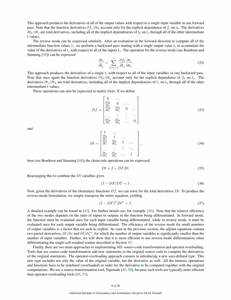
A. Single-Cell RoutineIn the previous work, the basis for the residual derivatives was a set of single-cell residual routines, developed fromthe original residual routines. These routines contained all of the functionality of the original block-based routines,including dissipation terms and boundary conditions, but were designed to operate on a 5 × 5 × 5 cell cube. This isthe smallest block of cells that encloses the second-order inviscid flux stencil, shown in Fig. 1. Evaluating this set ofroutines once produces the exact residuals for one cell in the mesh. These single-cell residual routines are generated

−3 −2 −1 0 1 2 3 −2−1

01

2−2.5

−2

−1.5

−1

−0.5

0

0.5

1

1.5

2

2.5

ji

k

Figure 1. Single-cell stencil

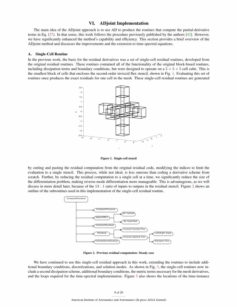
by cutting and pasting the residual computation from the original residual code, modifying the indices to limit theevaluation to a single stencil. This process, while not ideal, is less onerous than coding a derivative scheme fromscratch. Further, by reducing the residual computation to a single cell at a time, we significantly reduce the size ofthe differentiation problem, making reverse-mode differentiation more manageable. This is advantageous, as we willdiscuss in more detail later, because of the 13 : 1 ratio of inputs to outputs in the residual stencil. Figure 2 shows anoutline of the subroutines used in this implementation of the single-cell residual routine.

ComputeResidual

ComputePressure

ApplyAllBCs

InitializeResidual

Residual

VolumeNormalization

BC Farfield

BC EulerWall

Inviscid Central Flux

Inviscid Upwind Flux

Riemann Flux

Left/Right State

Figure 2. Previous residual computation: Steady case

We have continued to use this single-cell residual approach in this work, extending the routines to include addi-tional boundary conditions, discretizations, and solution modes. As shown in Fig. 3, the single-cell routines now in-clude a second dissipation scheme, additional boundary conditions, the metric terms necessary for the mesh derivatives,and the loops required for the time-spectral implementation. Figure 3 also shows the locations of the time-instance

9 of 20

American Institute of Aeronautics and Astronautics (In press-AIAA Journal)

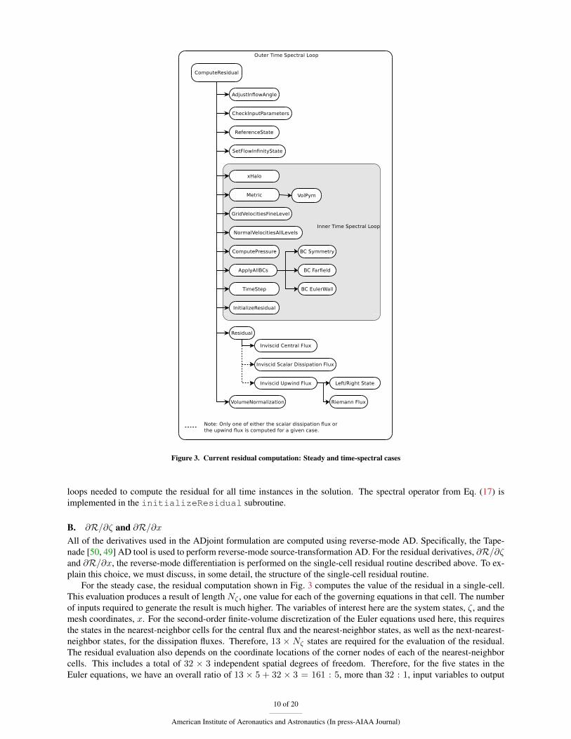
Figure 3. Current residual computation: Steady and time-spectral cases

loops needed to compute the residual for all time instances in the solution. The spectral operator from Eq. (17) isimplemented in the initializeResidual subroutine.

B. ∂R/∂ζ and ∂R/∂xAll of the derivatives used in the ADjoint formulation are computed using reverse-mode AD. Specifically, the Tape-nade [50, 49] AD tool is used to perform reverse-mode source-transformation AD. For the residual derivatives, ∂R/∂ζand ∂R/∂x, the reverse-mode differentiation is performed on the single-cell residual routine described above. To ex-plain this choice, we must discuss, in some detail, the structure of the single-cell residual routine.

For the steady case, the residual computation shown in Fig. 3 computes the value of the residual in a single-cell.This evaluation produces a result of length Nζ , one value for each of the governing equations in that cell. The numberof inputs required to generate the result is much higher. The variables of interest here are the system states, ζ, and themesh coordinates, x. For the second-order finite-volume discretization of the Euler equations used here, this requiresthe states in the nearest-neighbor cells for the central flux and the nearest-neighbor states, as well as the next-nearest-neighbor states, for the dissipation fluxes. Therefore, 13 × Nζ states are required for the evaluation of the residual.The residual evaluation also depends on the coordinate locations of the corner nodes of each of the nearest-neighborcells. This includes a total of 32 × 3 independent spatial degrees of freedom. Therefore, for the five states in theEuler equations, we have an overall ratio of 13 × 5 + 32 × 3 = 161 : 5, more than 32 : 1, input variables to output

10 of 20

American Institute of Aeronautics and Astronautics (In press-AIAA Journal)

variables. Even if we consider the fact that a single reverse-mode calculation is about 4.5 times more expensive thanthe equivalent forward evaluation of the single-cell routine, the reverse-mode calculation is still about 7 times fasterthan a forward computation for the single-cell routines.

In the time-spectral case, we must consider not only the spatial dependence of the operator but also its temporaldependence. In this discussion we refer to on-time-instance states and off-time-instance states. On-time-instance statesare those that exist in the same time instance as the current residual evaluation. Off-time-instance states are those thatexist in a time instance other than that associated with the current residual evaluation. In the case of a time-spectralsolution, the residual is dependent on the same on-time-instance states and coordinates as described above. In addition,it is dependent on the states and coordinates of the current cell on each of the off-time instances. Thus, we now haveNζ ×N residual values and (13×Nζ + 32× 3)×N + (Nζ + 8× 3)× (N − 1) input states and coordinates. Thisleads to a ratio of 36 : 1 input variables to output variables for the Euler equations with three time instances, a ratiothat increases as the number of time instances increases.

Note that both of these ratios include the state variable derivatives of ∂R/∂ζn as well as the coordinate derivativesof ∂R/∂x. This is possible because we have used reverse-mode AD for the derivative calculation. The reverseaccumulation, shown in Eq. (32), allows us to start with a single residual and, accumulating backwards through theroutines, calculate the derivatives of all the inputs at once. This turns out to be a significant advantage.

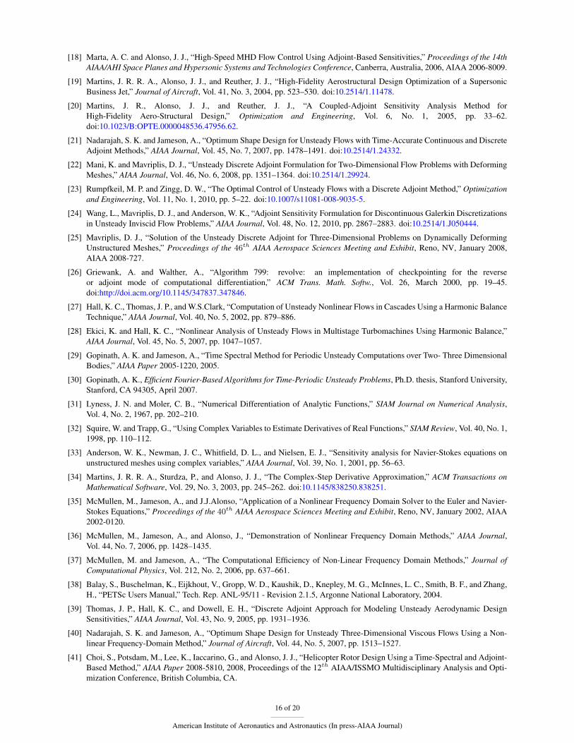
An important aspect of the expanded routine in the context of the time-spectral adjoint is the need for additionalloops to account for the extra time instances. As shown in Fig. 3, there are two time-instance loops in the spectralcomputation. The outer loop accounts for the time instances in the residual, and the inner loop accounts for the timeinstances of the states and coordinates. Therefore, we can see that the inner part of the computation scales with thenumber of instances squared, whereas the outer part scales with the number of instances. However, this is a somewhatnaive implementation of the single-cell routine. Examining Eq. (19) more closely, we notice that it is only the spectraloperator, V Dtζ

n, that contains states from all N time instances at one time. Therefore, we can reduce the numberof terms in the inner time-spectral loop to only those necessary for this term. Figure 4 shows this simplified routine.With this improved implementation, we have significantly reduced the number of computations needed in the innertime-spectral loop. Thus, the derivative computation now scales, essentially, with the number of time instances, N ,rather than N2. Timing results demonstrating this are presented in Section VII.

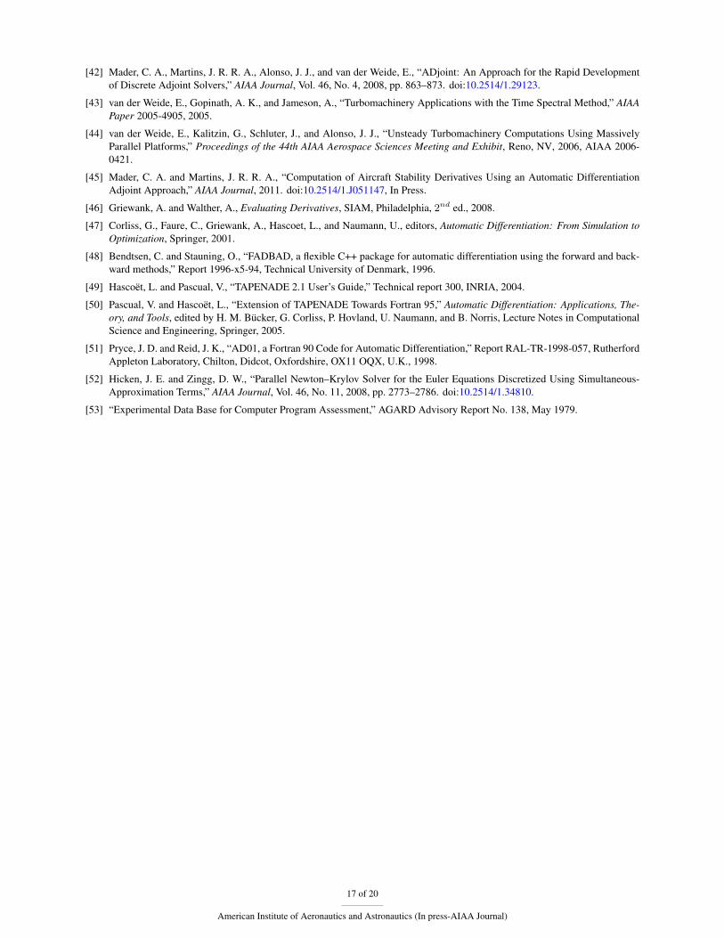
C. ∂I/∂ζ and ∂I/∂xFor most aerodynamic shape optimization problems, the objectives of interest are the forces and moments—or thecorresponding coefficients—acting on the body being optimized. Computing the partial derivatives of these quantitieswith respect to the states and mesh coordinates, ∂I/∂ζ and ∂I/∂x, is significantly simpler than the computation of theresidual partial derivatives. This is evident when we compare the routines required to compute the residual (Fig. 4) andthe routines required to compute the forces and moments (Fig. 5). As we can see from these figures, for the inviscidequations considered here, the force computation simply requires an integration of the pressure over the surface of thebody in question. This requires an application of the boundary conditions as well as a surface normal computation,but this is significantly simpler than the complicated flux computation required for the residual. Further, we can seethat the ratio of input variables to output variables strongly favors a reverse-mode technique for this computation. Fora typical optimization problem, we might be interested in fewer than ten force and moment coefficients—for example,CL and CD for a lift-constrained drag minimization—while the surface needed to compute those coefficients mayrequire hundreds, thousands, or even tens of thousands of surface cells for accurate discretization. This yields anextremely high ratio of input variables to output variables and thus strongly favors the reverse-mode approach. Asfor the residual routines, the force routines have been differentiated using the reverse-mode source-transformationcapabilities of Tapenade [50, 49]. This differentiation yields a routine that computes all the state and coordinatederivatives of a specified force or moment coefficient in a single pass.

The extension of this concept to the time-spectral case is relatively straightforward. We consider simple spectralobjectives, such as the average lift, drag, and moment coefficients. In these cases, the spectral objective is based onsimple algebraic combinations of the corresponding coefficient values at each of the discrete time instances in thesolution. For example, the average drag may be computed as

CD =1

NCD1

+1

NCD2

+ · · ·+ 1

NCDN (38)

where each of the coefficients CDi is computed directly from the states of time instance i. The time instances of theresidual computation are coupled through the spectral time derivative of Eq. (19), but once the solution is computed, thecomputations of the coefficients at each instance in time are independent. Therefore, provided the objective function

11 of 20

American Institute of Aeronautics and Astronautics (In press-AIAA Journal)

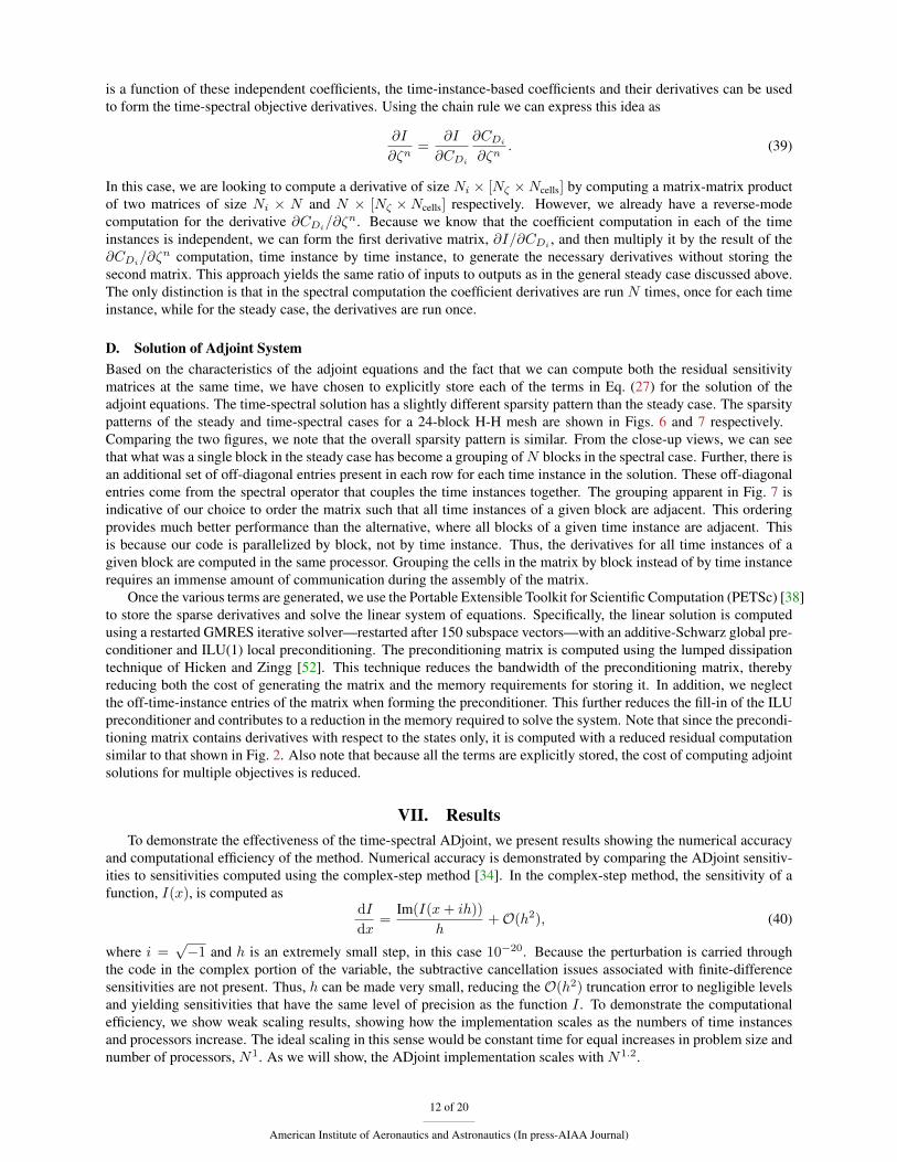
is a function of these independent coefficients, the time-instance-based coefficients and their derivatives can be usedto form the time-spectral objective derivatives. Using the chain rule we can express this idea as

∂I

∂ζn=

∂I

∂CDi

∂CDi∂ζn

. (39)

In this case, we are looking to compute a derivative of size Ni × [Nζ ×Ncells] by computing a matrix-matrix productof two matrices of size Ni × N and N × [Nζ ×Ncells] respectively. However, we already have a reverse-modecomputation for the derivative ∂CDi/∂ζ

n. Because we know that the coefficient computation in each of the timeinstances is independent, we can form the first derivative matrix, ∂I/∂CDi , and then multiply it by the result of the∂CDi/∂ζ

n computation, time instance by time instance, to generate the necessary derivatives without storing thesecond matrix. This approach yields the same ratio of inputs to outputs as in the general steady case discussed above.The only distinction is that in the spectral computation the coefficient derivatives are run N times, once for each timeinstance, while for the steady case, the derivatives are run once.

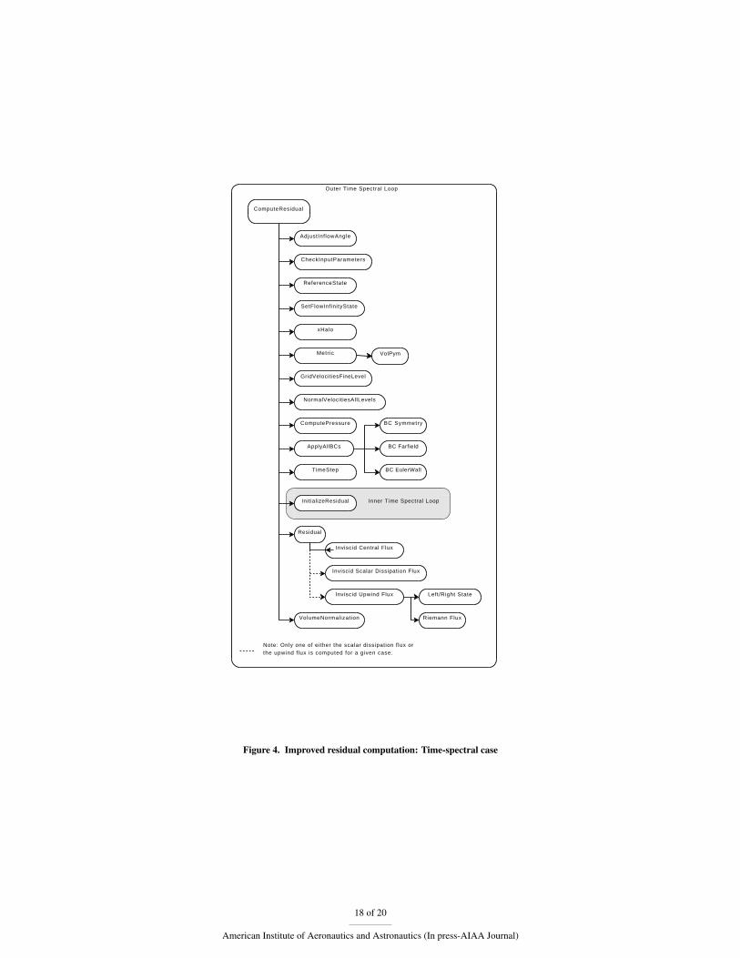
D. Solution of Adjoint SystemBased on the characteristics of the adjoint equations and the fact that we can compute both the residual sensitivitymatrices at the same time, we have chosen to explicitly store each of the terms in Eq. (27) for the solution of theadjoint equations. The time-spectral solution has a slightly different sparsity pattern than the steady case. The sparsitypatterns of the steady and time-spectral cases for a 24-block H-H mesh are shown in Figs. 6 and 7 respectively.Comparing the two figures, we note that the overall sparsity pattern is similar. From the close-up views, we can seethat what was a single block in the steady case has become a grouping ofN blocks in the spectral case. Further, there isan additional set of off-diagonal entries present in each row for each time instance in the solution. These off-diagonalentries come from the spectral operator that couples the time instances together. The grouping apparent in Fig. 7 isindicative of our choice to order the matrix such that all time instances of a given block are adjacent. This orderingprovides much better performance than the alternative, where all blocks of a given time instance are adjacent. Thisis because our code is parallelized by block, not by time instance. Thus, the derivatives for all time instances of agiven block are computed in the same processor. Grouping the cells in the matrix by block instead of by time instancerequires an immense amount of communication during the assembly of the matrix.

Once the various terms are generated, we use the Portable Extensible Toolkit for Scientific Computation (PETSc) [38]to store the sparse derivatives and solve the linear system of equations. Specifically, the linear solution is computedusing a restarted GMRES iterative solver—restarted after 150 subspace vectors—with an additive-Schwarz global pre-conditioner and ILU(1) local preconditioning. The preconditioning matrix is computed using the lumped dissipationtechnique of Hicken and Zingg [52]. This technique reduces the bandwidth of the preconditioning matrix, therebyreducing both the cost of generating the matrix and the memory requirements for storing it. In addition, we neglectthe off-time-instance entries of the matrix when forming the preconditioner. This further reduces the fill-in of the ILUpreconditioner and contributes to a reduction in the memory required to solve the system. Note that since the precondi-tioning matrix contains derivatives with respect to the states only, it is computed with a reduced residual computationsimilar to that shown in Fig. 2. Also note that because all the terms are explicitly stored, the cost of computing adjointsolutions for multiple objectives is reduced.

VII. ResultsTo demonstrate the effectiveness of the time-spectral ADjoint, we present results showing the numerical accuracy

and computational efficiency of the method. Numerical accuracy is demonstrated by comparing the ADjoint sensitiv-ities to sensitivities computed using the complex-step method [34]. In the complex-step method, the sensitivity of afunction, I(x), is computed as

dI

dx=

Im(I(x+ ih))

h+O(h2), (40)

where i =√−1 and h is an extremely small step, in this case 10−20. Because the perturbation is carried through

the code in the complex portion of the variable, the subtractive cancellation issues associated with finite-differencesensitivities are not present. Thus, h can be made very small, reducing the O(h2) truncation error to negligible levelsand yielding sensitivities that have the same level of precision as the function I . To demonstrate the computationalefficiency, we show weak scaling results, showing how the implementation scales as the numbers of time instancesand processors increase. The ideal scaling in this sense would be constant time for equal increases in problem size andnumber of processors, N1. As we will show, the ADjoint implementation scales with N1.2.

12 of 20

American Institute of Aeronautics and Astronautics (In press-AIAA Journal)

A. Test Case DescriptionTo benchmark the time-spectral ADjoint for accuracy, we compute the sensitivities for a 917,000 cell ONERA M6 [53]wing mesh. The wing is simulated with Euler wall surfaces and a symmetry plane at the root. The mesh has an H-Htopology with a nominal off-wall spacing of 0.002.

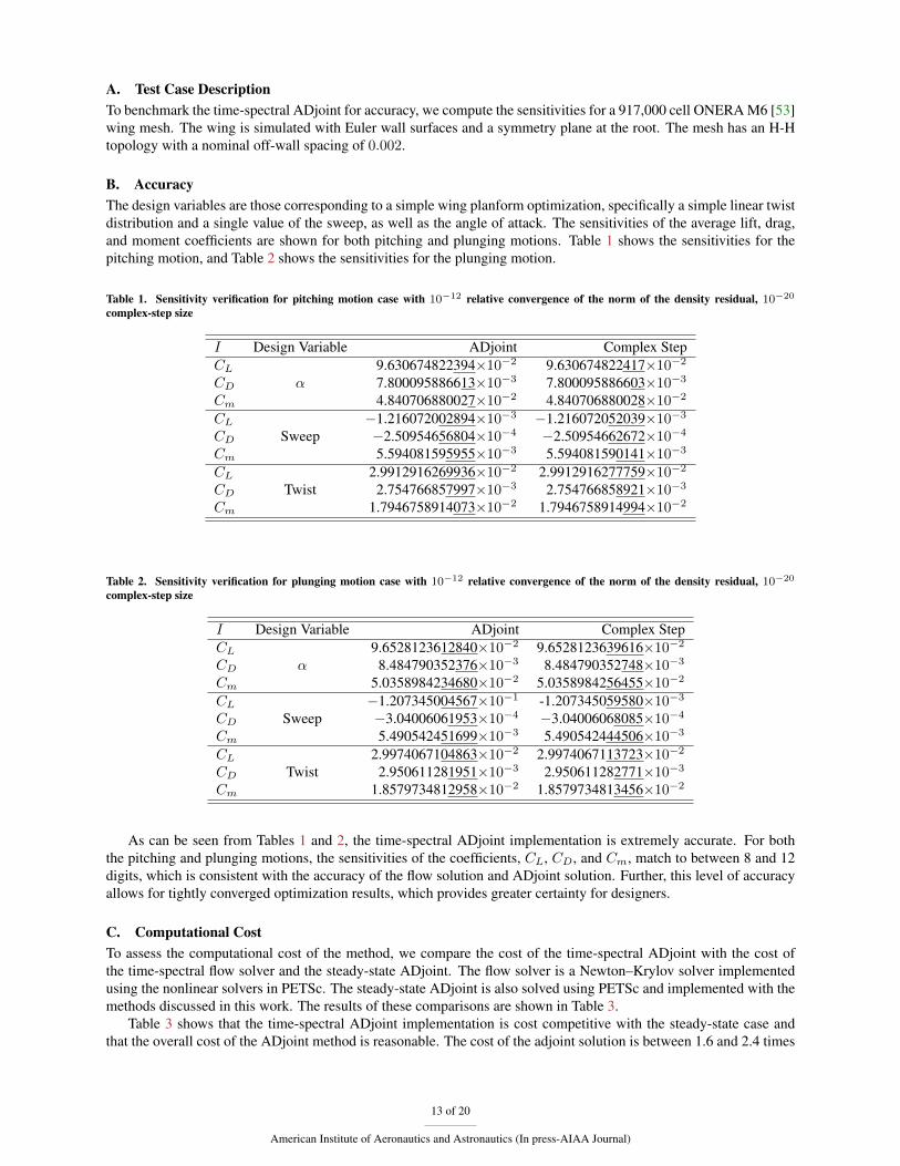
B. AccuracyThe design variables are those corresponding to a simple wing planform optimization, specifically a simple linear twistdistribution and a single value of the sweep, as well as the angle of attack. The sensitivities of the average lift, drag,and moment coefficients are shown for both pitching and plunging motions. Table 1 shows the sensitivities for thepitching motion, and Table 2 shows the sensitivities for the plunging motion.

Table 1. Sensitivity verification for pitching motion case with 10−12 relative convergence of the norm of the density residual, 10−20

complex-step size

I Design Variable ADjoint Complex StepCL 9.630674822394×10−2 9.630674822417×10−2

CD α 7.800095886613×10−3 7.800095886603×10−3

Cm 4.840706880027×10−2 4.840706880028×10−2

CL −1.216072002894×10−3 −1.216072052039×10−3

CD Sweep −2.50954656804×10−4 −2.50954662672×10−4

Cm 5.594081595955×10−3 5.594081590141×10−3

CL 2.9912916269936×10−2 2.9912916277759×10−2

CD Twist 2.754766857997×10−3 2.754766858921×10−3

Cm 1.7946758914073×10−2 1.7946758914994×10−2

Table 2. Sensitivity verification for plunging motion case with 10−12 relative convergence of the norm of the density residual, 10−20

complex-step size

I Design Variable ADjoint Complex StepCL 9.6528123612840×10−2 9.6528123639616×10−2

CD α 8.484790352376×10−3 8.484790352748×10−3

Cm 5.0358984234680×10−2 5.0358984256455×10−2

CL −1.207345004567×10−1 -1.207345059580×10−3

CD Sweep −3.04006061953×10−4 −3.04006068085×10−4

Cm 5.490542451699×10−3 5.490542444506×10−3

CL 2.9974067104863×10−2 2.9974067113723×10−2

CD Twist 2.950611281951×10−3 2.950611282771×10−3

Cm 1.8579734812958×10−2 1.8579734813456×10−2

As can be seen from Tables 1 and 2, the time-spectral ADjoint implementation is extremely accurate. For boththe pitching and plunging motions, the sensitivities of the coefficients, CL, CD, and Cm, match to between 8 and 12digits, which is consistent with the accuracy of the flow solution and ADjoint solution. Further, this level of accuracyallows for tightly converged optimization results, which provides greater certainty for designers.

C. Computational CostTo assess the computational cost of the method, we compare the cost of the time-spectral ADjoint with the cost ofthe time-spectral flow solver and the steady-state ADjoint. The flow solver is a Newton–Krylov solver implementedusing the nonlinear solvers in PETSc. The steady-state ADjoint is also solved using PETSc and implemented with themethods discussed in this work. The results of these comparisons are shown in Table 3.

Table 3 shows that the time-spectral ADjoint implementation is cost competitive with the steady-state case andthat the overall cost of the ADjoint method is reasonable. The cost of the adjoint solution is between 1.6 and 2.4 times

13 of 20

American Institute of Aeronautics and Astronautics (In press-AIAA Journal)

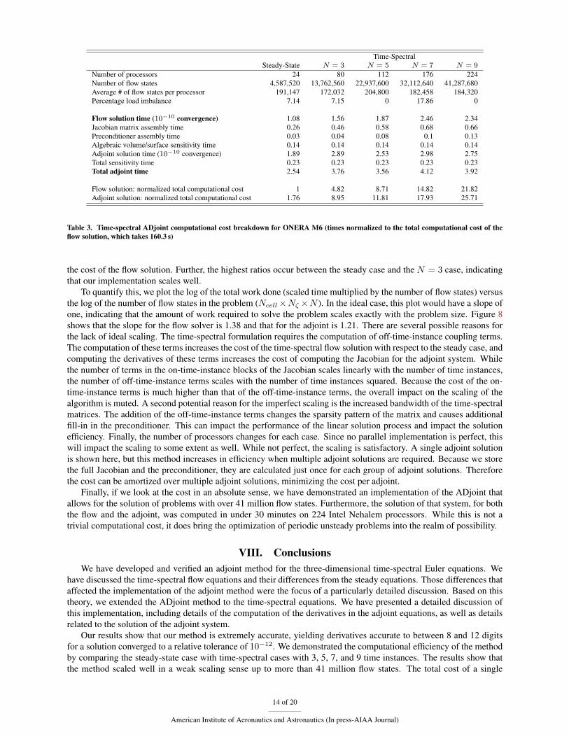
Time-SpectralSteady-State N = 3 N = 5 N = 7 N = 9

Number of processors 24 80 112 176 224Number of flow states 4,587,520 13,762,560 22,937,600 32,112,640 41,287,680Average # of flow states per processor 191,147 172,032 204,800 182,458 184,320Percentage load imbalance 7.14 7.15 0 17.86 0

Flow solution time (10−10 convergence) 1.08 1.56 1.87 2.46 2.34Jacobian matrix assembly time 0.26 0.46 0.58 0.68 0.66Preconditioner assembly time 0.03 0.04 0.08 0.1 0.13Algebraic volume/surface sensitivity time 0.14 0.14 0.14 0.14 0.14Adjoint solution time (10−10 convergence) 1.89 2.89 2.53 2.98 2.75Total sensitivity time 0.23 0.23 0.23 0.23 0.23Total adjoint time 2.54 3.76 3.56 4.12 3.92

Flow solution: normalized total computational cost 1 4.82 8.71 14.82 21.82Adjoint solution: normalized total computational cost 1.76 8.95 11.81 17.93 25.71

Table 3. Time-spectral ADjoint computational cost breakdown for ONERA M6 (times normalized to the total computational cost of theflow solution, which takes 160.3 s)

the cost of the flow solution. Further, the highest ratios occur between the steady case and the N = 3 case, indicatingthat our implementation scales well.

To quantify this, we plot the log of the total work done (scaled time multiplied by the number of flow states) versusthe log of the number of flow states in the problem (Ncell×Nζ ×N ). In the ideal case, this plot would have a slope ofone, indicating that the amount of work required to solve the problem scales exactly with the problem size. Figure 8shows that the slope for the flow solver is 1.38 and that for the adjoint is 1.21. There are several possible reasons forthe lack of ideal scaling. The time-spectral formulation requires the computation of off-time-instance coupling terms.The computation of these terms increases the cost of the time-spectral flow solution with respect to the steady case, andcomputing the derivatives of these terms increases the cost of computing the Jacobian for the adjoint system. Whilethe number of terms in the on-time-instance blocks of the Jacobian scales linearly with the number of time instances,the number of off-time-instance terms scales with the number of time instances squared. Because the cost of the on-time-instance terms is much higher than that of the off-time-instance terms, the overall impact on the scaling of thealgorithm is muted. A second potential reason for the imperfect scaling is the increased bandwidth of the time-spectralmatrices. The addition of the off-time-instance terms changes the sparsity pattern of the matrix and causes additionalfill-in in the preconditioner. This can impact the performance of the linear solution process and impact the solutionefficiency. Finally, the number of processors changes for each case. Since no parallel implementation is perfect, thiswill impact the scaling to some extent as well. While not perfect, the scaling is satisfactory. A single adjoint solutionis shown here, but this method increases in efficiency when multiple adjoint solutions are required. Because we storethe full Jacobian and the preconditioner, they are calculated just once for each group of adjoint solutions. Thereforethe cost can be amortized over multiple adjoint solutions, minimizing the cost per adjoint.

Finally, if we look at the cost in an absolute sense, we have demonstrated an implementation of the ADjoint thatallows for the solution of problems with over 41 million flow states. Furthermore, the solution of that system, for boththe flow and the adjoint, was computed in under 30 minutes on 224 Intel Nehalem processors. While this is not atrivial computational cost, it does bring the optimization of periodic unsteady problems into the realm of possibility.

VIII. ConclusionsWe have developed and verified an adjoint method for the three-dimensional time-spectral Euler equations. We

have discussed the time-spectral flow equations and their differences from the steady equations. Those differences thataffected the implementation of the adjoint method were the focus of a particularly detailed discussion. Based on thistheory, we extended the ADjoint method to the time-spectral equations. We have presented a detailed discussion ofthis implementation, including details of the computation of the derivatives in the adjoint equations, as well as detailsrelated to the solution of the adjoint system.

Our results show that our method is extremely accurate, yielding derivatives accurate to between 8 and 12 digitsfor a solution converged to a relative tolerance of 10−12. We demonstrated the computational efficiency of the methodby comparing the steady-state case with time-spectral cases with 3, 5, 7, and 9 time instances. The results show thatthe method scaled well in a weak scaling sense up to more than 41 million flow states. The total cost of a single

14 of 20

American Institute of Aeronautics and Astronautics (In press-AIAA Journal)

adjoint was approximately twice that of a flow solution. For a workload of approximately 180,000 flow states perprocessor, a flow solution and an adjoint solution can be computed in under 30 minutes. Thus, the optimization ofperiodic unsteady problems is now feasible.

AcknowledgmentsThe authors are grateful for the funding provided by the Natural Sciences and Engineering Research Council. The

computations were performed on the general purpose cluster supercomputer at the SciNet high performance computingconsortium. SciNet is funded by the Canada Foundation for Innovation under the auspices of Compute Canada, theGovernment of Ontario, Ontario Research Fund—Research Excellence, and the University of Toronto. The authorswould like to thank Edwin van der Weide and Juan J. Alonso for their assistance in the early stages of this project, inparticular with respect to the time-spectral CFD formulation in the SUmb flow solver. The authors would also like tothank Gaetan Kenway for his assistance in improving the efficiency of the steady-state ADjoint.

ReferencesReferences

[1] Pironneau, O., “On Optimum Design in Fluid Mechanics,” Journal of Fluid Mechanics, Vol. 64, 1974, pp. 97–110.

[2] Jameson, A., “Aerodynamic Design via Control Theory,” Journal of Scientific Computing, Vol. 3, No. 3, sep 1988, pp. 233–260.

[3] Nemec, M. and Zingg, D. W., “Newton—Krylov Algorithm for Aerodynamic Design Using the Navier–Stokes Equations,”AIAA Journal, Vol. 40, No. 6, June 2002, pp. 1146–1154.

[4] Anderson, W. K. and Venkatakrishnan, V., “Aerodynamic design optimization on unstructured grids with a continuous adjointformulation,” Computers and Fluids, Vol. 28, No. 4-5, 1999, pp. 443–480.

[5] Anderson, W. K. and Bonhaus, D. L., “Airfoil Design on Unstructured Grids for Turbulent Flows,” AIAA Journal, Vol. 37,No. 2, 1999, pp. 185–191.

[6] Soemarwoto, B. I. and Labrujere, T. E., “AIRFOIL DESIGN AND OPTIMIZATION METHODS:RECENT PROGRESS ATNLR,” International Journal for Numerical Methods in Fluids, Vol. 30, No. 2, 1999, pp. 217–228.

[7] Driver, J. and Zingg, D. W., “Numerical Aerodynamic Optimization Incorporating Laminar-Turbulent Transition Prediction,”AIAA Journal, Vol. 45, No. 8, 2007, pp. 1810–1818.

[8] Nemec, M., Zingg, D. W., and Pulliam, T. H., “Multipoint and Multi-Objective Aerodynamic Shape Optimization,” AIAAJournal, Vol. 42, No. 6, 2004, pp. 1057–1065.

[9] Jameson, A., “Optimum Aerodynamic Design Using Control Theory,” Computational Fluid Dynamics Review, 1995, pp. 495–528.

[10] Hicken, J. E. and Zingg, D. W., “Induced-Drag Minimization of Nonplanar Geometries Based on the Euler Equations,” AIAAJournal, Vol. 48, No. 11, 2010, pp. 2564–2575. doi:10.2514/1.J050379.

[11] Jameson, A., Martinelli, L., and Pierce, N. A., “Optimum Aerodynamic Design Using the Navier-Stokes Equations,” Theo-retical and Computational Fluid Dynamics, Vol. 10, 1998, pp. 213–237.

[12] Nielsen, E. J. and Anderson, W. K., “Aerodynamic Design Optimization on Unstructured Meshes Using the Navier-StokesEquations,” AIAA Journal, Vol. 37, No. 11, 1999, pp. 1411–1419.

[13] Buckley, H. P., Zhou, B. Y., and Zingg, D. W., “Airfoil Optimization Using Practical Aerodynamic Design Requirements,”Journal of Aircraft, Vol. 47, No. 5, 2010, pp. 1707–1719. doi:10.2514/1.C000256.

[14] Reuther, J. J., Jameson, A., Alonso, J. J., , Rimlinger, M. J., and Saunders, D., “Constrained Multipoint Aerodynamic ShapeOptimization Using an Adjoint Formulation and Parallel Computers, Part 1,” Journal of Aircraft, Vol. 36, No. 1, 1999, pp. 51–60.

[15] Reuther, J. J., Jameson, A., Alonso, J. J., , Rimlinger, M. J., and Saunders, D., “Constrained Multipoint Aerodynamic ShapeOptimization Using an Adjoint Formulation and Parallel Computers, Part 2,” Journal of Aircraft, Vol. 36, No. 1, 1999, pp. 61–74.

[16] Nadarajah, S. K., Jameson, A., and Alonso, J. J., “Sonic Boom Reduction using an Adjoint Method for Wing-Body Configu-rations in Supersonic Flow,” AIAA Paper 2002-5547, 2002.

[17] Marta, A. C., Mader, C. A., Martins, J. R. R. A., van der Weide, E., and Alonso, J. J., “A methodology for the developmentof discrete adjoint solvers using automatic differentiation tools,” International Journal of Computational Fluid Dynamics,Vol. 21, No. 9, 2007, pp. 307–327.

15 of 20

American Institute of Aeronautics and Astronautics (In press-AIAA Journal)

[18] Marta, A. C. and Alonso, J. J., “High-Speed MHD Flow Control Using Adjoint-Based Sensitivities,” Proceedings of the 14thAIAA/AHI Space Planes and Hypersonic Systems and Technologies Conference, Canberra, Australia, 2006, AIAA 2006-8009.

[19] Martins, J. R. R. A., Alonso, J. J., and Reuther, J. J., “High-Fidelity Aerostructural Design Optimization of a SupersonicBusiness Jet,” Journal of Aircraft, Vol. 41, No. 3, 2004, pp. 523–530. doi:10.2514/1.11478.

[20] Martins, J. R., Alonso, J. J., and Reuther, J. J., “A Coupled-Adjoint Sensitivity Analysis Method forHigh-Fidelity Aero-Structural Design,” Optimization and Engineering, Vol. 6, No. 1, 2005, pp. 33–62.doi:10.1023/B:OPTE.0000048536.47956.62.

[21] Nadarajah, S. K. and Jameson, A., “Optimum Shape Design for Unsteady Flows with Time-Accurate Continuous and DiscreteAdjoint Methods,” AIAA Journal, Vol. 45, No. 7, 2007, pp. 1478–1491. doi:10.2514/1.24332.

[22] Mani, K. and Mavriplis, D. J., “Unsteady Discrete Adjoint Formulation for Two-Dimensional Flow Problems with DeformingMeshes,” AIAA Journal, Vol. 46, No. 6, 2008, pp. 1351–1364. doi:10.2514/1.29924.

[23] Rumpfkeil, M. P. and Zingg, D. W., “The Optimal Control of Unsteady Flows with a Discrete Adjoint Method,” Optimizationand Engineering, Vol. 11, No. 1, 2010, pp. 5–22. doi:10.1007/s11081-008-9035-5.

[24] Wang, L., Mavriplis, D. J., and Anderson, W. K., “Adjoint Sensitivity Formulation for Discontinuous Galerkin Discretizationsin Unsteady Inviscid Flow Problems,” AIAA Journal, Vol. 48, No. 12, 2010, pp. 2867–2883. doi:10.2514/1.J050444.

[25] Mavriplis, D. J., “Solution of the Unsteady Discrete Adjoint for Three-Dimensional Problems on Dynamically DeformingUnstructured Meshes,” Proceedings of the 46th AIAA Aerospace Sciences Meeting and Exhibit, Reno, NV, January 2008,AIAA 2008-727.

[26] Griewank, A. and Walther, A., “Algorithm 799: revolve: an implementation of checkpointing for the reverseor adjoint mode of computational differentiation,” ACM Trans. Math. Softw., Vol. 26, March 2000, pp. 19–45.doi:http://doi.acm.org/10.1145/347837.347846.

[27] Hall, K. C., Thomas, J. P., and W.S.Clark, “Computation of Unsteady Nonlinear Flows in Cascades Using a Harmonic BalanceTechnique,” AIAA Journal, Vol. 40, No. 5, 2002, pp. 879–886.

[28] Ekici, K. and Hall, K. C., “Nonlinear Analysis of Unsteady Flows in Multistage Turbomachines Using Harmonic Balance,”AIAA Journal, Vol. 45, No. 5, 2007, pp. 1047–1057.

[29] Gopinath, A. K. and Jameson, A., “Time Spectral Method for Periodic Unsteady Computations over Two- Three DimensionalBodies,” AIAA Paper 2005-1220, 2005.

[30] Gopinath, A. K., Efficient Fourier-Based Algorithms for Time-Periodic Unsteady Problems, Ph.D. thesis, Stanford University,Stanford, CA 94305, April 2007.

[31] Lyness, J. N. and Moler, C. B., “Numerical Differentiation of Analytic Functions,” SIAM Journal on Numerical Analysis,Vol. 4, No. 2, 1967, pp. 202–210.

[32] Squire, W. and Trapp, G., “Using Complex Variables to Estimate Derivatives of Real Functions,” SIAM Review, Vol. 40, No. 1,1998, pp. 110–112.

[33] Anderson, W. K., Newman, J. C., Whitfield, D. L., and Nielsen, E. J., “Sensitivity analysis for Navier-Stokes equations onunstructured meshes using complex variables,” AIAA Journal, Vol. 39, No. 1, 2001, pp. 56–63.

[34] Martins, J. R. R. A., Sturdza, P., and Alonso, J. J., “The Complex-Step Derivative Approximation,” ACM Transactions onMathematical Software, Vol. 29, No. 3, 2003, pp. 245–262. doi:10.1145/838250.838251.

[35] McMullen, M., Jameson, A., and J.J.Alonso, “Application of a Nonlinear Frequency Domain Solver to the Euler and Navier-Stokes Equations,” Proceedings of the 40th AIAA Aerospace Sciences Meeting and Exhibit, Reno, NV, January 2002, AIAA2002-0120.

[36] McMullen, M., Jameson, A., and Alonso, J., “Demonstration of Nonlinear Frequency Domain Methods,” AIAA Journal,Vol. 44, No. 7, 2006, pp. 1428–1435.

[37] McMullen, M. and Jameson, A., “The Computational Efficiency of Non-Linear Frequency Domain Methods,” Journal ofComputational Physics, Vol. 212, No. 2, 2006, pp. 637–661.

[38] Balay, S., Buschelman, K., Eijkhout, V., Gropp, W. D., Kaushik, D., Knepley, M. G., McInnes, L. C., Smith, B. F., and Zhang,H., “PETSc Users Manual,” Tech. Rep. ANL-95/11 - Revision 2.1.5, Argonne National Laboratory, 2004.

[39] Thomas, J. P., Hall, K. C., and Dowell, E. H., “Discrete Adjoint Approach for Modeling Unsteady Aerodynamic DesignSensitivities,” AIAA Journal, Vol. 43, No. 9, 2005, pp. 1931–1936.

[40] Nadarajah, S. K. and Jameson, A., “Optimum Shape Design for Unsteady Three-Dimensional Viscous Flows Using a Non-linear Frequency-Domain Method,” Journal of Aircraft, Vol. 44, No. 5, 2007, pp. 1513–1527.

[41] Choi, S., Potsdam, M., Lee, K., Iaccarino, G., and Alonso, J. J., “Helicopter Rotor Design Using a Time-Spectral and Adjoint-Based Method,” AIAA Paper 2008-5810, 2008, Proceedings of the 12th AIAA/ISSMO Multidisciplinary Analysis and Opti-mization Conference, British Columbia, CA.

16 of 20

American Institute of Aeronautics and Astronautics (In press-AIAA Journal)

[42] Mader, C. A., Martins, J. R. R. A., Alonso, J. J., and van der Weide, E., “ADjoint: An Approach for the Rapid Developmentof Discrete Adjoint Solvers,” AIAA Journal, Vol. 46, No. 4, 2008, pp. 863–873. doi:10.2514/1.29123.

[43] van der Weide, E., Gopinath, A. K., and Jameson, A., “Turbomachinery Applications with the Time Spectral Method,” AIAAPaper 2005-4905, 2005.

[44] van der Weide, E., Kalitzin, G., Schluter, J., and Alonso, J. J., “Unsteady Turbomachinery Computations Using MassivelyParallel Platforms,” Proceedings of the 44th AIAA Aerospace Sciences Meeting and Exhibit, Reno, NV, 2006, AIAA 2006-0421.

[45] Mader, C. A. and Martins, J. R. R. A., “Computation of Aircraft Stability Derivatives Using an Automatic DifferentiationAdjoint Approach,” AIAA Journal, 2011. doi:10.2514/1.J051147, In Press.

[46] Griewank, A. and Walther, A., Evaluating Derivatives, SIAM, Philadelphia, 2nd ed., 2008.

[47] Corliss, G., Faure, C., Griewank, A., Hascoet, L., and Naumann, U., editors, Automatic Differentiation: From Simulation toOptimization, Springer, 2001.

[48] Bendtsen, C. and Stauning, O., “FADBAD, a flexible C++ package for automatic differentiation using the forward and back-ward methods,” Report 1996-x5-94, Technical University of Denmark, 1996.

[49] Hascoet, L. and Pascual, V., “TAPENADE 2.1 User’s Guide,” Technical report 300, INRIA, 2004.

[50] Pascual, V. and Hascoet, L., “Extension of TAPENADE Towards Fortran 95,” Automatic Differentiation: Applications, The-ory, and Tools, edited by H. M. Bucker, G. Corliss, P. Hovland, U. Naumann, and B. Norris, Lecture Notes in ComputationalScience and Engineering, Springer, 2005.

[51] Pryce, J. D. and Reid, J. K., “AD01, a Fortran 90 Code for Automatic Differentiation,” Report RAL-TR-1998-057, RutherfordAppleton Laboratory, Chilton, Didcot, Oxfordshire, OX11 OQX, U.K., 1998.

[52] Hicken, J. E. and Zingg, D. W., “Parallel Newton–Krylov Solver for the Euler Equations Discretized Using Simultaneous-Approximation Terms,” AIAA Journal, Vol. 46, No. 11, 2008, pp. 2773–2786. doi:10.2514/1.34810.

[53] “Experimental Data Base for Computer Program Assessment,” AGARD Advisory Report No. 138, May 1979.

17 of 20

American Institute of Aeronautics and Astronautics (In press-AIAA Journal)

AdjustInflowAngle

ComputeResidual

CheckInputParameters

ReferenceState

SetFlowInfinityState

xHalo

Metric

Inner Time Spectral Loop

GridVelocitiesFineLevel

NormalVelocitiesAllLevels

ComputePressure

ApplyAllBCs

TimeStep

InitializeResidual

Residual

VolumeNormalization

VolPym

BC Symmetry

BC Farfield

BC EulerWall

Inviscid Central Flux

Inviscid Scalar Dissipation Flux

Inviscid Upwind Flux

Riemann Flux

Left/Right State

Outer Time Spectral Loop

Note: Only one of either the scalar dissipation flux orthe upwind f lux is computed for a given case.

Figure 4. Improved residual computation: Time-spectral case

18 of 20

American Institute of Aeronautics and Astronautics (In press-AIAA Journal)

ComputeSurfacePressures

ComputeForces

ComputeSurfaceNormals

ComputeForcesAndMoments

GetSurfaceCoordinates

ApplyAllBCs

AdjustInflowAngle

ComputeCoefficients

BC EulerWall

Figure 5. Force and moment computation

Figure 6. Steady case sparsity pattern: 24-block H-H mesh

19 of 20

American Institute of Aeronautics and Astronautics (In press-AIAA Journal)

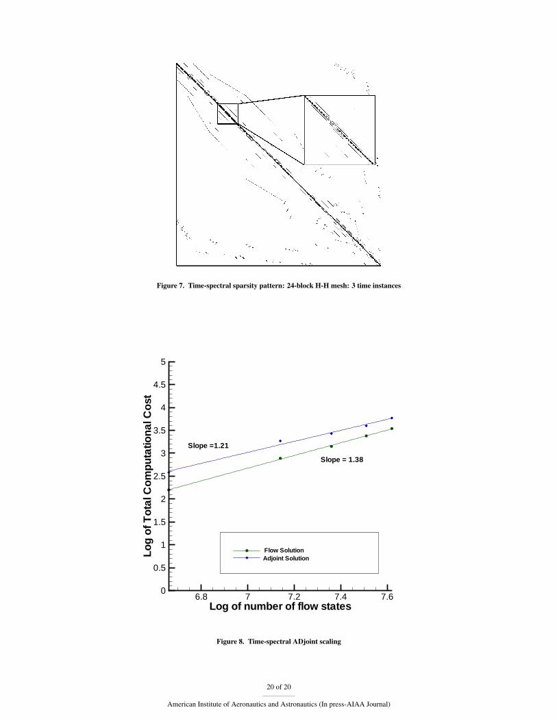
Figure 7. Time-spectral sparsity pattern: 24-block H-H mesh: 3 time instances

Log of number of flow states

Log

ofT

otal

Com

puta

tiona

lCos

t

6.8 7 7.2 7.4 7.60

0.5

1

1.5

2

2.5

3

3.5

4

4.5

5

Slope =1.21

Slope = 1.38

Flow SolutionAdjoint Solution

Figure 8. Time-spectral ADjoint scaling

20 of 20

American Institute of Aeronautics and Astronautics (In press-AIAA Journal)