Derivation of the Navier–Stokes equationsFrom Wikipedia, the free encyclopedia

The intent of this article is to highlight the important points of the derivation of the Navier–Stokes equations as well as the application and formulation for different families offluids.

Contents

  [hide] 

1 Basic assumptions 2 The material derivative 3 Conservation laws

o 3.1 Conservation of momentumo 3.2 Conservation of mass

4 General form of the equations of motion 5 Application to different fluids

o 5.1 Newtonian fluid 5.1.1 Compressible Newtonian fluid 5.1.2 Incompressible Newtonian fluid

o 5.2 Non-Newtonian fluidso 5.3 Bingham fluido 5.4 Power-law fluid

6 Stream function formulationo 6.1 2D flow in orthogonal coordinates

7 The stress tensor 8 Notes 9 References

Basic assumptions[edit]

The Navier–Stokes equations are based on the assumption that the fluid, at the scale of interest, is a continuum, in other words is not made up of discrete particles but rather a continuous substance. Another necessary assumption is that all the fields of interest like pressure, velocity, density, and temperature are differentiable, weakly at least.

The equations are derived from the basic principles of conservation of mass, momentum, and energy. For that matter, sometimes it is necessary to consider a finite arbitrary volume, called a control volume, over which these principles can be applied. This finite volume is denoted by   and its bounding surface  . The control volume can remain fixed in space or can move with the fluid.

The material derivative[edit]

Main article: material derivative

Changes in properties of a moving fluid can be measured in two different ways. One can measure a given property by either carrying out the measurement on a fixed point in space as particles of the fluid pass by, or by following a parcel of fluid along its streamline. The derivative of a field with respect to a fixed position in space is called the Eulerianderivative while the derivative following a moving parcel is called the advective or material ("Lagrangian" [1]) derivative.

The material derivative is defined as the operator:

where   is the velocity of the fluid. The first term on the right-hand side of the equation is the ordinary Eulerian derivative (i.e. the derivative on a fixed reference frame, representing changes at a point with respect to time) whereas the second term represents changes of a quantity with respect to position (see advection). This "special" derivative is in fact the ordinary derivative of a function of many variables along a path following the fluid motion; it may be derived through application of the chain rule in which all independent variables are checked for change along the path (i.e. the total derivative).

For example, the measurement of changes in wind velocity in the atmosphere can be obtained with the help of an anemometer in a weather station or by observing the movement of a weather balloon. The anemometer in the first case is measuring the velocity of all the moving particles passing through a fixed point in space, whereas in the second case the instrument is measuring changes in velocity as it moves with the fluid.

Conservation laws[edit]

The Navier–Stokes equation is a special case of the (general) continuity equation. It, and associated equations such as mass continuity, may be derived from conservation principles of:

Mass Momentum Energy .

This is done via the Reynolds transport theorem, an integral solution relation stating that the sum of the changes of some intensive property (call it  ) defined over a control volume   must be equal to what is lost (or gained) through the boundaries of the volume plus what is created/consumed by sources and sinks inside the control volume. This is expressed by the following integral equation:

where v is the velocity of the fluid and   represents the sources and sinks in the fluid, taking the sinks as positive. Recall that   represents the control volume and   its bounding surface.

The divergence theorem may be applied to the surface integral, changing it into a volume integral:

Applying Leibniz's rule to the integral on the left and then combining all of the integrals:

The integral must be zero for any control volume; this can only be true if the integrand itself is zero, so that:

From this valuable relation (a very generic continuity equation), three important concepts may be concisely written: conservation of mass, conservation of momentum, and conservation of energy. Validity is retained if   is a vector, in which case the vector-vector product in the second term will be a dyad.

Conservation of momentum[edit]

The most elemental form of the Navier–Stokes equations is obtained when the conservation relation is applied to momentum. Writing momentum as   gives:

where   is a dyad, a special case of tensor product, which results in a second rank tensor; the divergence of a second rank tensor is again a vector (a first rank tensor).[2]Noting that a body force (notated  ) is a source or sink of momentum (per volume) and expanding the derivatives completely:

Note that the gradient of a vector is a special case of the covariant derivative, the operation results in second rank tensors;[2] except in Cartesian coordinates, it's important to understand that this isn't simply an element by element gradient. Rearranging and recognizing

that  :

The leftmost expression enclosed in parentheses is, by mass continuity (shown in a moment), equal to zero. Noting that what remains on the right side of the equation is theconvective derivative:

This appears to simply be an expression of Newton's second law (F = ma) in terms of body forces instead of point forces. Each term in any case of the Navier–Stokes equations is a body force. A shorter though less rigorous way to arrive at this result would be the application of the chain rule to acceleration:

where  . The reason why this is "less rigorous" is that we haven't shown that

picking   is correct; however it does make sense since with that choice of path the derivative is "following" a fluid "particle", and in order for Newton's second law to work, forces must be summed following a particle. For this reason theconvective derivative is also known as the particle derivative.

Conservation of mass[edit]

Mass may be considered also. Taking   (no sources or sinks of mass) and putting in density:

where   is the mass density (mass per unit volume), and   is the velocity of the fluid. This equation is called the mass continuity equation, or simply "the" continuity equation. This equation generally accompanies the Navier–Stokes equation.

In the case of an incompressible fluid,   is a constant and the equation reduces to:

which is in fact a statement of the conservation of volume.

General form of the equations of motion[edit]

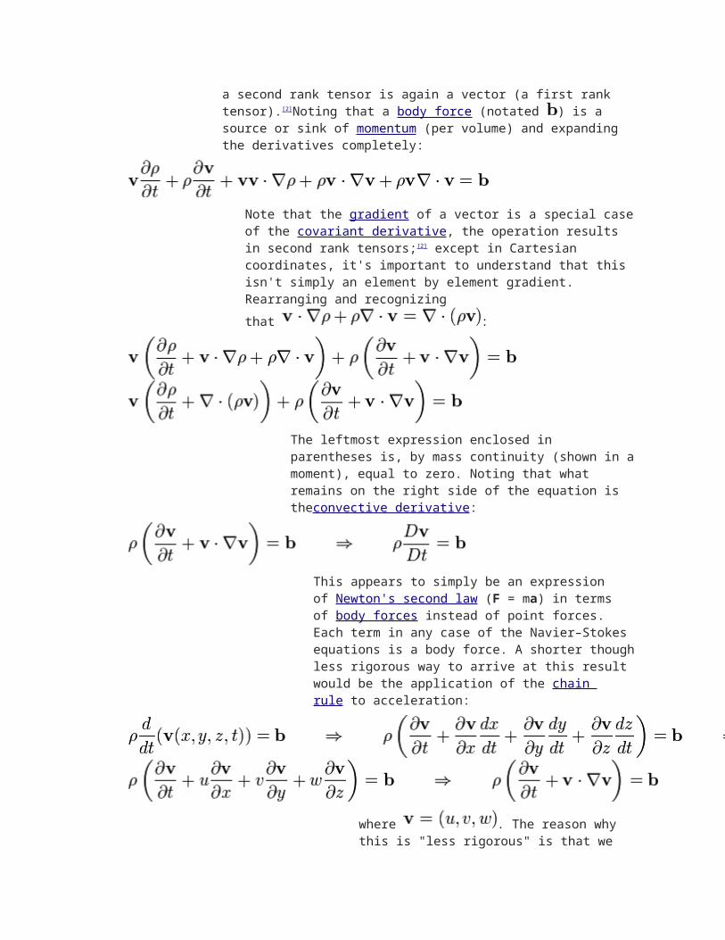
The generic body force   seen previously is made specific first by breaking it up into two new terms, one to describe forces resulting from stresses and one for "other" forces such as gravity. By examining the forces acting on a small cube in a fluid, it may be shown that

where   is the Cauchy stress tensor, and   accounts for other body forces present. This equation is called the Cauchy momentum equation and describes the non-relativistic momentum conservation of any continuum that conserves mass.   is a rank two symmetric tensor given by its covariant components:

where the   are normal stresses and   shear stresses. This tensor is split up into two terms:

where   is the 3 x 3 identity matrix and   is the deviatoric stress tensor. Note that the mechanical pressure π is equal to minus the mean normal stress:[3]

The motivation for doing this is that pressure is typically a variable of interest, and also this simplifies application to specific fluid families later on since the rightmost tensor   in the equation above must be zero for a fluid at rest. Note that   is traceless. The Navier–Stokes equation may now be written in the most general form:

This equation is still incomplete. For completion, one must make hypotheses on the forms of   and , that is, one needs a constitutive law for the stress tensor which can be obtained for specific fluid families and on the pressure; additionally, if the flow is assumed compressible an equation of state will be required, which will likely further require a conservation of energy formulation.

Application to different fluids[edit]

The general form of the equations of motion is not "ready for use", the stress tensor is still unknown so that more information is needed; this information is normally some knowledge of the viscous behavior of the fluid. For different types of fluid flow this results in specific forms of the Navier–Stokes equations.

Newtonian fluid[edit]Main article: Newtonian fluid

Compressible Newtonian fluid[edit]

The formulation for Newtonian fluids stems from an observation made by Newton that, for most fluids,

In order to apply this to the Navier–Stokes equations, three assumptions were made by Stokes:

The stress tensor is a linear function of the strain rates. The fluid is isotropic. For a fluid at rest,   must be zero (so that hydrostatic pressure results).

Applying these assumptions will lead to:

That is, the deviatoric of the deformation rate tensor is identified to the deviatoric of the stress tensor, up to a factor μ.[4]

 is the Kronecker delta. μ a

nd λ are proportionality constants associated with the assumption that stress depends on strain linearly; μ is called the first coefficient of viscosity(usually just called "viscosity") and λ is the second coefficient of viscosity (related to bulk viscosity). The value of λ, which produces a viscous effect associated with volume change, is very difficult to determine, not even its sign is known with absolute certainty. Even in

compressible flows, the term involving λ is often negligible; however it can occasionally be important even in nearly incompressible flows and is a matter of controversy. When taken nonzero, the most common approximation is λ ≈ - ⅔ μ.[5]

A straightforward substituti

on of   into the momentum conservation equation will yield the Navier–Stokes equations for a compressible Newtonian fluid:

or, more compactly in vector form,

where the transpose has been used. Gravity has been accounted for as "the" body force, i.e. 

. The associated mass continuity equation is:

In addition to this equation, an equation of state and an equation for the conservation of energy is needed. The equation of state to use depends on context (often the ideal gas law), the conservation of energy will read:

Here,   is the enthalpy, 

 is the temperature, and   is a function representing the dissipation of energy due to viscous effects:

With a good equation of state and good functions

for the dependence of parameters (such as viscosity) on the variables, this system of equations seems to properly model the dynamics of all known gases and most liquids.

Incompressible Newtonian fluid[edit]

For the special (but very common) case of incompressible flow, the momentum equations simplify significantly. Taking into account the following assumptions:

Viscosity   now be a constant

The second viscosity effect 

The simplified mass continuity equation 

then looking at the viscous terms of the   momentum equation for example we have:

Similarly for the and   momentum directions we

have   

and  .

Non-Newtonian fluids[edit]Main article: Non-Newtonian fluid

A non-Newtonian fluid is a fluid whose flow properties differ in any way from those of Newtonian fluidsMost commonly the viscosity of non-Newtonian fluids is not independent ofshear rate or shear rate history. However, there are some non-Newtonian fluids with shear-independent viscosity, that nonetheless exhibit normal stress-differences or other non-Newtonian behaviour. Many salt solutions and molten polymers

non-Newtonian fluids, as are many commonly found substances such as ketchup, custardothpaste, starch suspensions, paintod, and shampooNewtonian fluid, the relation between the shear stressthe shear rate is linear, passing through the origin, the constant of proportionality being the coefficient of viscosity. In a non-Newtonian fluid, the relation between the shear stress and the shear rate is different, and can even be time-dependent. The study of the non-Newtonian fluids is usually called rheology. A few examples are given here.

Bingham fluidMain article: Bingham plastic

In Bingham fluids, the situation is slightly different:

These are fluids capable of bearing some shear before they start flowing. Some common examples are toothpaste and

Power-law fluidMain article: Power-law fluid

A power law fluid is an idealised fluid for which the shear stressby

This form is useful for approximating all sorts of general fluids, including shear thinning (such as latex paint) and shear thickening (such as corn starch water mixture).

Stream function formulationIn the analysis of a flow, it is often desirable to reduce the number of equations or the number of variables being dealt with, or both. The incompressible Navier-Stokes equation with mass continuity (four equations in four unknowns) can, in fact, be reduced to a single equation with a single dependent variable in 2D, or one vector equation in 3D. This is enabled by two vector calculus identities:

for any differentiable scalarvector  . The first identity implies that any term in the Navier-Stokes equation that may be represented as the gradient of a scalar will disappear when the curl of the equation is taken. Commonly, pressure and gravity are what eliminate, resulting in (this is true in 2D as well as 3D):

where it's assumed that all body forces are describable as gradients (true for gravity), and density has been divided so that viscosity becomes

The second vector calculus identity above states that the divergence of the curl of a

vector field is zero. Since the (incompressible) mass continuity equation specifies the divergence of velocity being zero, we can replace the velocity with the

curl of some vectorcontinuity is always satisfied:

So, as long as velocity is represented

through unconditionally satisfied. With this new dependent vector variable, the Navier-Stokes equation (with curl taken as above) becomes a single fourth order vector equation, no longer containing the unknown pressure variable and no longer dependent on a separate mass continuity equation:

Apart from containing fourth order derivatives, this equation is fairly complicated, and is thus uncommon. Note that if the cross differentiation is left out, the result is a third order vector equation containing an unknown vector field (the gradient of pressure) that may be determined from the same boundary conditions that one would apply to the fourth order equation above.

2D flow in orthogonal coordinates

The true utility of this formulation is seen when the flow is two dimensional in nature and the equation is written in a generalother words a system where the basis vectors are orthogonal. Note that this by no means limits application to Cartesian coordinatesthe common coordinates systems are orthogonal, including familiar ones likeones like toroidal

The 3D velocity is expressed as (note that the discussion has been coordinate free up till now):

where   are basis vectors, not necessarily constant and not necessarily normalized, andcomponents; let also the coordinates of space

be 

Now suppose that the flow is 2D. This doesn't mean the flow is in a plane, rather it means that the component of velocity in one direction is zero and the remaining components are independent of the same direction. In that case (take component 3 to be zero):

The vector function

but this must simplify in some way also since the flow is assumed 2D. If orthogonal coordinates are assumed, thesimple form, and the equation above expanded becomes:

Examining this equation shows that we can setretain equality with no loss of generality, so that:

the significance here is that only one component offlow becomes a problem with only one dependent variable. The cross differentiated Navier–Stokes equation becomes two 0 = 0 equations and one meaningful equation.

The remaining component

equation for   can simplify since a variety of quantities will now equal zero, for example:

if the scale factorsdefinition of the 

Manipulating the cross differentiated Navier–Stokes equation using the above two equations and a variety of identitiesthe stream function:

where   is thecontained scalar equation that describes both momentum and mass conservation in 2D. The only other equations that thisboundary conditions.

[show]Derivation of the scalar stream function equation

The assumptions for the stream function equation are listed below:

The flow is incompressible and Newtonian. Coordinates are

Flow is 2D:  The first two scale factors of the coordinate system are independent of the last

coordinate: 

The stream function

Since negative of the Laplacian of the stream function.

The level curves

The stress tensorThe derivation of the Navier-Stokes equation involves the consideration of forces acting on fluid elements, so that a quantity called themomentum equationthe equation fully simplified, so that the original appearance of the stress tensor is lost.

However, the stress tensor still has some important uses, especially in formulating boundary conditions at fluid interfacestensor is:

If the fluid is assumed to be incompressible, the tensor simplifies significantly:

 is the strain rate