Future Generation Computer Systems 25 (2009) 617–626

Contents lists available at ScienceDirect

Future Generation Computer Systems

journal homepage: www.elsevier.com/locate/fgcs

Derivation of self-scheduling algorithms for heterogeneous distributed computersystems: Application to internet-based grids of computersJavier Díaz, Sebastián Reyes, Alfonso Niño, Camelia Muñoz-Caro ∗Grupo de Química Computacional y Computación de Alto Rendimiento, Escuela Superior de Informática, Universidad de Castilla-La Mancha, Paseo de la Universidad 4,13071, Ciudad Real, Spain

a r t i c l e i n f o

Article history:Received 27 May 2008Received in revised form4 December 2008Accepted 13 December 2008Available online 27 December 2008

Keywords:Self-scheduling algorithmsLoad balancingComputational gridDistributed systems

a b s t r a c t

Self-scheduling algorithms are useful for achieving load balance in heterogeneous computational systems.Therefore, they can be applied in computational Grids. Here, we introduce two families of self-schedulingalgorithms. The first considers an explicit form for the chunks distribution function. The second focuseson the variation rate of the chunks distribution function. From the first family, we propose a QuadraticSelf-Scheduling (QSS) algorithm. From the second, two newalgorithms, Exponential Self-Scheduling (ESS)and Root Self-Scheduling (RSS) are introduced. QSS, ESS and RSS are tested in an Internet-based Grid ofComputers involving resources from Spain andMexico. QSS and ESS outperform previous self-schedulingalgorithms. QSS is found slightly more efficient than ESS. RSS shows a poor performance, a fact tracedback to the curvature of the chunks distribution function.

© 2009 Elsevier B.V. All rights reserved.

1. Introduction

Workload distribution is an important issue in distributedsystems. Efficient allocation of the workload among processorsis necessary to optimize the use of the computational resources.This is specially important when the resources are not onlydistributed, but also heterogeneous, as in a computationalGrid [1]. A computational Grid is a hardware and softwareinfrastructure providing dependable, consistent, and pervasiveaccess to resources among different administrative domains. Inthis form, we allow the sharing of the resources in a unifiedway, maximizing their use. A Grid can be used to perform large-scale runs of distributed applications. To minimize the overallcomputing time, a correct assignment of tasks is needed, so thatcomputer loads and communication overheads are well balanced.In this context, scheduling algorithms are needed. Differentscheduling strategies have been developed along the years (for theclassical taxonomy see [2]). In particular, dynamic self-schedulingalgorithms are extensively used in practical applications. Thesealgorithms represent adaptive schemes where tasks are allocatedin run-time. Self-scheduling algorithmswere initially developed tosolve parallel loop scheduling problems in homogeneousmemory-shared systems, see for instance [3]. Here, the loop iterations have

∗ Corresponding author.E-mail addresses: javier.diaz@uclm.es (J. Díaz), sebastian.reyes@uclm.es

(S. Reyes), alfonso.nino@uclm.es (A. Niño), camelia.munoz@uclm.es(C. Muñoz-Caro).

0167-739X/$ – see front matter© 2009 Elsevier B.V. All rights reserved.doi:10.1016/j.future.2008.12.003

not interdependencies, and they can be scheduled as independenttasks. Despite their origin, these algorithms have been testedsuccessfully in distributed memory multiprocessor systems andheterogeneous clusters [4–14]. In addition, someworks about theirperformance on Grid connected clusters of computers have alsobeen reported [15–19].In the general case, a computational Grid can be thought

of as a dynamic heterogeneous distributed system. Here, bydynamic, as opposed to static, we mean that the characteristicsdefining the system are not fixed. In particular, the availabilityand performance of computer nodes (CPUs) and network links canchange over the time. From this standpoint, a suitable strategy tothe development of efficient Grid scheduling strategies is to startby deriving efficient scheduling schemes for static heterogeneousdistributed computer systems. Later, the dynamic behaviour ofthe system can be incorporated into the parameters defining theschemes. Therefore, as core components of more efficient Gridscheduling models, in this work we present new self-schedulingschemes. Thus, two general families of self-scheduling algorithmsare developed. From these families, new flexible self-schedulingalgorithms, oriented toward heterogeneous distributed systems,are derived. These algorithms are compared with prior self-scheduling strategies in a dedicated, static, heterogeneous Grid ofcomputers.The rest of this paper is organized as follows: Section 2

presents an overview of self-scheduling algorithms.; In Section 3,we introduce two families of self-scheduling algorithms, andnew self-scheduling schemes are presented; Section 4 detailsthe methodology used for comparing the new approaches with

618 J. Díaz et al. / Future Generation Computer Systems 25 (2009) 617–626

well-established self-scheduling schemes; Section 5 presents andinterprets the results found in the comparative study. Finally, inSection 6 we present the main conclusions of this paper, and inSection 7 the perspectives for future works.

2. Background

When trying to allocate a set of tasks among several proces-sors we have two complementary effects: load balance and com-munication overhead. The theoretical work of Kruskal and Weiss[20] showed that two extreme scheduling models correspond tothe optimization of one of these factors. On one hand, we havestatic chunking. This method assigns a task to each idle proces-sor achieving good load balance but causing toomuch communica-tion and scheduling overhead. On the other hand, we have ChunkSelf-Scheduling (CSS) [21], which divides the total number of tasksamong the available processors, assigning the resulting number oftasks (the chunk) to each processor. Here, we achieve low over-head, but load imbalance will be important if the tasks use differ-ent computing times. The practical self-scheduling schemes lookfor an equilibrium between load balance and overhead. In this con-text, Kruskal and Weiss [20] showed that an appropriate strategyis to use a number of chunks higher than the number of processors,assigning a decreasing number of tasks to each processor as it be-comes free. On this basis, several self-scheduling algorithms havebeen proposed.The simplest of these algorithms is Guided Self-Scheduling

(GSS), which dynamically changes the number of tasks assigned toeachprocessor [22].More specifically, the chunk size is determinedby dividing the number of remaining tasks by the total numberof processors. In this form, the chunk size decreases in eachchunk, achieving good load balancing and reducing the schedulingoverhead. However, in the early chunks GSS may assign too manytasks to the processors, and the remaining tasks may not besufficient to guarantee a good load balance.On the other hand, we have Factoring Self-Scheduling (FSS) that

results froma statistical analysiswhere the computing time in eachprocessor is considered an independent random variable. Here, thetasks are scheduled in batches (or stages) of P chunks of equalsize, where P is the number of processors [23]. The chunk sizeis determined by dividing the number of remaining tasks by theproduct of the number of processors and by a parameter (α). Thisparameter ensures that the total number of tasks per batch is afixed ratio of those remaining, i.e., only a subset of the remainingtasks (usually half) is scheduled in each batch. This algorithmprovides better workload balance than GSS when task executiontimes vary widely and unpredictably. The overhead of FSS is notsignificantly greater than that of GSS.Another approach is Trapezoid Self-Scheduling (TSS). TSS uses

a linear decreasing chunk function [24]. In this form, the algorithmtries to reduce the scheduling overhead, since the function issimple and minimizes the need for synchronization. In addition,the decreasing chunk sizes balance the workload. TSS assignsF and L tasks to the first and last chunk, respectively. F and Lare parameters adjustable by the programmer. Tzen and Ni [24]proposed as suboptimal values F = I/2P and L = 1, being I thetotal number of tasks and P the available processors.Self-scheduling algorithms are derived for homogeneous sys-

tems but, in principle, they can be applied to heterogeneous onessuch as computational Grids. However, they could be not enoughflexible (they have not enough degrees of freedom) to adapt ef-ficiently to this heterogeneous and dynamic environment. Differ-ent algorithms have been proposed for this case, such as AffinityScheduling (AS) [25]. AS combines static and dynamic schedul-ing strategies. Other approaches introduce additional degrees offreedom in the model. Thus, we have proposed previously a newself-scheduling algorithm called Quadratic Self-Scheduling (QSS)

[14,18]. This algorithm is based on a quadratic form for the chunksdistribution function. Therefore,we have three degrees of freedom,which provide higher adaptability to heterogeneous distributedsystems. A different approach is to take into account the environ-ment characteristics. Here, most of the algorithms are based ina master-slave architecture, where the master obtains the infor-mation necessary to allocate the different tasks among the slaves.Thus, Weighted Factoring (WF) uses a variant of Factoring Self-Scheduling, which incorporates weight factors for each processor(slave) [26]. These factors are experimentally determined from therelative computing power of the processors. In WF each proces-sor weight remains constant throughout the parallel execution.Banicescu and Liu [27] have proposed a method called AdaptiveFactoring (AF). AF adjusts the processors weights according to tim-ing information reflecting variations in the available computingpower of the slaves. Chronopoulos et al. [11] extended the TSS al-gorithm, proposing the Distributed TSS (DTSS). In this algorithm,chunks sizes are weighted by the relative power of the server pro-cessors and by the number of processes in their run-queue at themoment of requesting work from the master. Ciorba et al. ex-tended in [28] the DTSS algorithm, proposing DTSS+ SP to handleloops with dependencies on heterogeneous clusters via synchro-nization points (SPs). In [12], Chronopoulos et al. proposed a Hier-archical DTSS (HDTSS). This is a hierarchical method, which triesto avoid the bottleneck problems of the centralized schemes likeDTSS. Also, there are self-scheduling algorithms based on the his-tory of task timing results, like SAS [29]. This self-scheduling algo-rithm attempts to balance dynamically the applicationworkload inthe presence of a fluctuating exogenous load. SAS assigns chunksaccording to the history of previous timing results, to the history ofall incoming tasks, and to the current number of processes in therun-queue. Another approach, based in Guided Self-Scheduling, isGap-Aware Self-Scheduling (GAS) [30]. Here, a temporal gap fac-tor for each processor is calculated, measuring its availability. De-pending on these factors the algorithm modifies the chunk sizecalculated by GSS. Finally, there is another kind of self-schedulingalgorithms that can redistribute the workload when a load imbal-ance is detected, for example RAS [4]. This is an algorithm thatusing a master-slaves model estimates the computational perfor-mance of the slaves. The tasks are distributed among the slave pro-cessors depending on the performance estimates. However, themaster can redistribute tasks when a load imbalance is detected.Other approach is TREES [31,7]. This is a distributed load bal-ancing scheme that statically arranges the processors in a logicalcommunication topology based on the computing powers of theprocessors involved. When a processor becomes idle, it asks forwork from a single, predefined partner, which migrates half itswork to the idle processor.As the above examples show, self-scheduling algorithms are at

the core of more refined techniques for task scheduling in Gridenvironments. Therefore, new, more efficient algorithms are ofinterest for defining new Grid scheduling approaches.

3. New Self-Scheduling Schemes

This section presents two different families of Self-Schedulingmethods. As usual [24], they are derived using a continuous chunksdistribution function, C(t). This function gives the chunk size as afunction of the t-chunk. The first family is based in the chunks dis-tribution function,whereas the second focuses on the slope of C(t).

3.1. Methods based in the chunks distribution function

Any continuous function can be approached by a Taylor series.This represents a polynomial approach to the function around agiven point. The larger the expansion, the better the approach.

J. Díaz et al. / Future Generation Computer Systems 25 (2009) 617–626 619

Therefore, we can use a Taylor expansion of arbitrary order forapproaching the chunks distribution function C(t) in the followingform. Consider, using the nomenclature of Tzen and Ni [24], anarbitrary parallel system composed by P processors with a total ofI tasks to schedule. As in reference [24], we define a job as a unit ofwork assigned to a processor (i.e., a group or chunk, composed by acertain number of tasks). Let C(t) be the chunk function giving thechunk size for the t-th chunk, with t defined in the interval [0,N].Themain strategy is to assign each chunk to the next free processorin the system.Two conditions must be fulfilled for any form of C(t). First, the

exigency of a decreasing chunk size requires,

dC(t)dt

< 0. (1)

This condition means that C(t) is a monotonic decreasing functionand, therefore,

C(tb) ≤ C(ta) ∀tb > ta ∈ [0,N]. (2)

The second condition is that the number of tasks I is fixed. Thistranslates into,

I =∫ N

0C(t)dt. (3)

Let us consider C(t) to be anunspecified function of t : C(t) = f (t).This function can be proposed ad hoc or it can be derived froma set of assumptions. As examples of these two cases we haveGuided Self-Scheduling [22] and Factoring Self-Scheduling [23],respectively.In this work, we introduce another approach to determine C(t).

C(t) can be expressed by a Taylor expansion. In this way, assumingthat C(t) is n-derivable in a point ta ∈ [0,N], we can build a Taylorpolynomial P(t) of n order [32],

P(t) =n∑k=0

Ck(ta)k!

(t − ta)k (4)

where,

Ck(ta) =dkC(ta)dtn

(5)

and

C0(ta) = ta (6)

P(t) is an approximation to C(t) and, therefore:

C(t) = P(t)+ En(t) =n∑k=0

Ck(ta)k!

(t − ta)k + En(t) (7)

where En(t) = C(t) − P(t) is the approximation error. TheEq. (7) defines the Taylor formula with remainder [32]. It can beshown [32] that

En(t) =1n!

∫ t

ta(t − s)nC (n+1)(s)ds (8)

fromwhich it is deduced [32] that, given two valuesm andM suchas,

m ≤ C (n+1)(t) ≤ M ∀t ∈ [0,N] (9)

then

m(t − ta)n+1

(n+ 1)!≤ En(t) ≤ M

(t − ta)n+1

(n+ 1)!if t > ta (10)

and

m(ta − t)n+1

(n+ 1)!≤ (−1)n+1En(t) ≤ M

(t − ta)n+1

(n+ 1)!if ta > t (11)

Eqs. (10) and (11) represent a bracketing of the error. They showthat the error is reduced (it depends inversely on (n + 1)!) whenthe terms of the polynomial P(t) are increased. This conclusionwill be applied to our treatment. Approximating C(t) by a Taylorpolynomial we have

C(t) ' C(t0)+[dC(t)dt

]t0

(t − t0)

+12

[d2C(t)dt2

]t0

(t − t0)2 + · · · (12)

or in a more compact form,

C(t) ' a+ bt + ct2 + · · · . (13)

Limiting the expansion of Eq. (13) to the constant term, we haveeither the Pure Self-Scheduling (a = 1) or the Chunk Self-Scheduling (a = I/P) algorithm. A less approximate model isobtained retaining up to the linear term. This case correspondsto the Trapezoid Self-Scheduling algorithm. Here, we can obtainthe C(t) function with a couple of (C(t), t) points. The first (C0, 0)and last (CN ,N) points used in the TSS algorithm are (I/2P, 0)and (1,N), respectively. These points were chosen as conservativevalues to keep between bounds the load balance [24]. Using thesepoints, we have that Eq. (13) reduces for a linear expansion to.

C(t) = C0 +(CN − C0)N

t (14)

where CN = 1 and C0 = I/2P . This result is equivalent to thatderived in Reference [24].Different algorithms can be obtained by retaining additional

terms of the Taylor expansion. For the quadratic case we haveQuadratic Self-Scheduling [14,18,19].

3.1.1. Quadratic Self-Scheduling (QSS)If we retain up to the quadratic term of the Taylor expansion

(13), we obtain, in the sense of Eqs. (10) and (11), a more flexibleand less approximate model than the TSS algorithm. In this case,

C(t) = a+ bt + ct2 (15)

where t represents the t-th chunk assigned to a processor. To applythe QSS algorithm we need the a, b and c coefficients of Eq. (15).The most direct solution, albeit approximate, is to select threereference points (C(t), t) and using Eq. (13) solve for the resultingsystem of equations. In previous studies [14,18,19], the two firstpoints were selected as in the TSS linear case, that is (I/2P, 0) and(1,N). The third point is selected as (CN/2,N/2), where N/2 is halfthe number of chunks for the quadratic case. CN/2 can be any valuein the interval [C0, CN ]. Solving the system of equations for a, b andc , we obtain,

a = C0b = (4CN/2 − CN − 3C0)/N

c = (2C0 + 2CN − 4CN/2)/N2(16)

where N is obtained by applying Eq. (3), which yields,

N = 6I/(4CN/2 + CN + C0) (17)

On the other hand, the CN/2 value is given by,

CN/2 =CN + C0δ

(18)

and since C0 and CN are fixed, the CN/2 value determines the slopeof Eq. (15) at a given point. Therefore, depending on δ, the slope ofthe quadratic function for a fixed t is higher or smaller than thatof the linear case (TSS algorithm), which corresponds to δ = 2.

620 J. Díaz et al. / Future Generation Computer Systems 25 (2009) 617–626

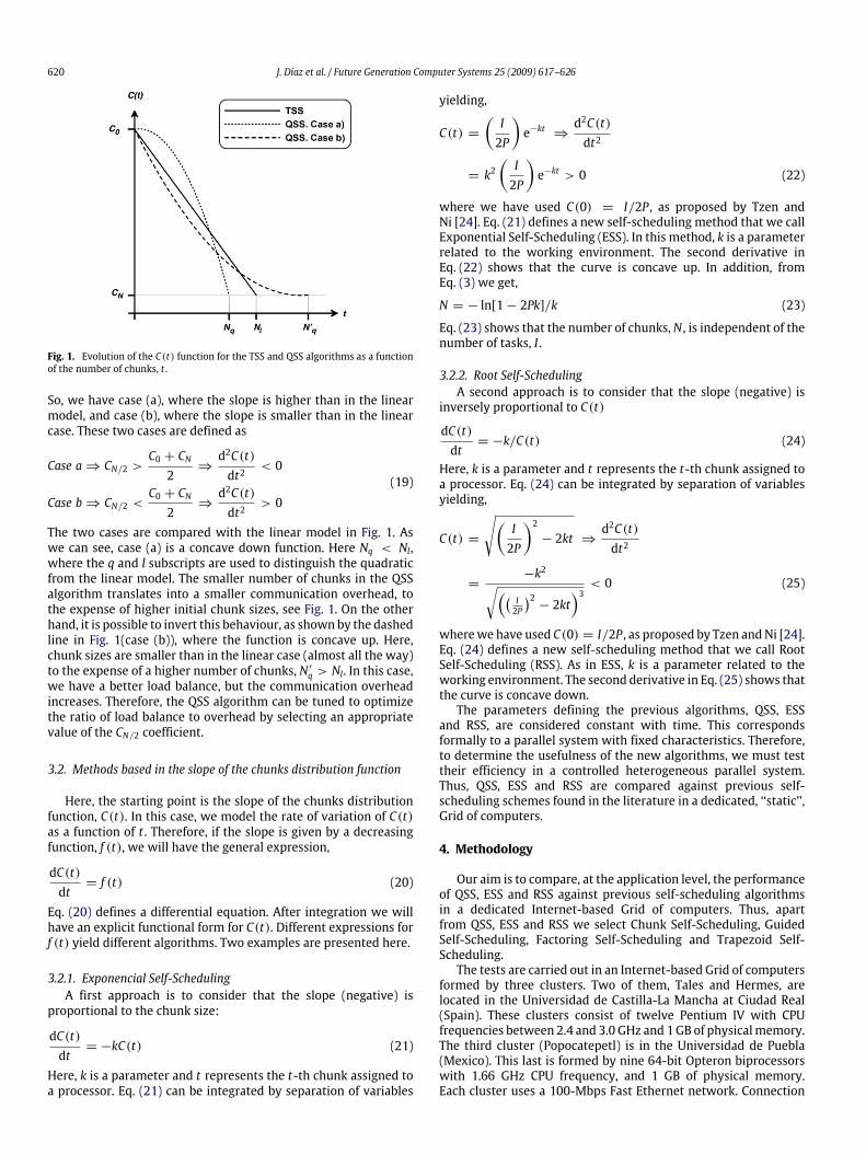
Fig. 1. Evolution of the C(t) function for the TSS and QSS algorithms as a functionof the number of chunks, t .

So, we have case (a), where the slope is higher than in the linearmodel, and case (b), where the slope is smaller than in the linearcase. These two cases are defined as

Case a⇒ CN/2 >C0 + CN2

⇒d2C(t)dt2

< 0

Case b⇒ CN/2 <C0 + CN2

⇒d2C(t)dt2

> 0(19)

The two cases are compared with the linear model in Fig. 1. Aswe can see, case (a) is a concave down function. Here Nq < Nl,where the q and l subscripts are used to distinguish the quadraticfrom the linear model. The smaller number of chunks in the QSSalgorithm translates into a smaller communication overhead, tothe expense of higher initial chunk sizes, see Fig. 1. On the otherhand, it is possible to invert this behaviour, as shown by the dashedline in Fig. 1(case (b)), where the function is concave up. Here,chunk sizes are smaller than in the linear case (almost all the way)to the expense of a higher number of chunks, N ′q > Nl. In this case,we have a better load balance, but the communication overheadincreases. Therefore, the QSS algorithm can be tuned to optimizethe ratio of load balance to overhead by selecting an appropriatevalue of the CN/2 coefficient.

3.2. Methods based in the slope of the chunks distribution function

Here, the starting point is the slope of the chunks distributionfunction, C(t). In this case, we model the rate of variation of C(t)as a function of t . Therefore, if the slope is given by a decreasingfunction, f (t), we will have the general expression,

dC(t)dt= f (t) (20)

Eq. (20) defines a differential equation. After integration we willhave an explicit functional form for C(t). Different expressions forf (t) yield different algorithms. Two examples are presented here.

3.2.1. Exponencial Self-SchedulingA first approach is to consider that the slope (negative) is

proportional to the chunk size:

dC(t)dt= −kC(t) (21)

Here, k is a parameter and t represents the t-th chunk assigned toa processor. Eq. (21) can be integrated by separation of variables

yielding,

C(t) =(I2P

)e−kt ⇒

d2C(t)dt2

= k2(I2P

)e−kt > 0 (22)

where we have used C(0) = I/2P , as proposed by Tzen andNi [24]. Eq. (21) defines a new self-scheduling method that we callExponential Self-Scheduling (ESS). In this method, k is a parameterrelated to the working environment. The second derivative inEq. (22) shows that the curve is concave up. In addition, fromEq. (3) we get,

N = − ln[1− 2Pk]/k (23)

Eq. (23) shows that the number of chunks, N , is independent of thenumber of tasks, I .

3.2.2. Root Self-SchedulingA second approach is to consider that the slope (negative) is

inversely proportional to C(t)

dC(t)dt= −k/C(t) (24)

Here, k is a parameter and t represents the t-th chunk assigned toa processor. Eq. (24) can be integrated by separation of variablesyielding,

C(t) =

√(I2P

)2− 2kt ⇒

d2C(t)dt2

=−k2√(( I

2P

)2− 2kt

)3 < 0 (25)

wherewe have used C(0) = I/2P , as proposed by Tzen andNi [24].Eq. (24) defines a new self-scheduling method that we call RootSelf-Scheduling (RSS). As in ESS, k is a parameter related to theworking environment. The second derivative in Eq. (25) shows thatthe curve is concave down.The parameters defining the previous algorithms, QSS, ESS

and RSS, are considered constant with time. This correspondsformally to a parallel system with fixed characteristics. Therefore,to determine the usefulness of the new algorithms, we must testtheir efficiency in a controlled heterogeneous parallel system.Thus, QSS, ESS and RSS are compared against previous self-scheduling schemes found in the literature in a dedicated, ‘‘static’’,Grid of computers.

4. Methodology

Our aim is to compare, at the application level, the performanceof QSS, ESS and RSS against previous self-scheduling algorithmsin a dedicated Internet-based Grid of computers. Thus, apartfrom QSS, ESS and RSS we select Chunk Self-Scheduling, GuidedSelf-Scheduling, Factoring Self-Scheduling and Trapezoid Self-Scheduling.The tests are carried out in an Internet-based Grid of computers

formed by three clusters. Two of them, Tales and Hermes, arelocated in the Universidad de Castilla-La Mancha at Ciudad Real(Spain). These clusters consist of twelve Pentium IV with CPUfrequencies between 2.4 and 3.0 GHz and 1GB of physicalmemory.The third cluster (Popocatepetl) is in the Universidad de Puebla(Mexico). This last is formed by nine 64-bit Opteron biprocessorswith 1.66 GHz CPU frequency, and 1 GB of physical memory.Each cluster uses a 100-Mbps Fast Ethernet network. Connection

J. Díaz et al. / Future Generation Computer Systems 25 (2009) 617–626 621

between clusters is achieved through Internet. The Grid usesGlobus as basic middleware in its 4.0.3 flavour [33,34]. To allocatethe tasks on the Grid we use the 5.0 version of the GridWaymetascheduler [35,36] through its DRMAA API [37,38].The different parameters of the self-scheduling algorithms have

been configured as follows. In Chunk Self-Scheduling, the chunksize is by definition given as the quotient of tasks to processors. Onthe other hand, Guided Self-Scheduling determines the chunk sizeat each step using the number of tasks and available processors.In Factoring Self-Scheduling, we have used a value of 2 for the αparameter, the optimal value obtained in the original statisticalanalysis of the FSS method [23]. In Trapezoid Self-Scheduling wehave used the optimal values found by Tzen and Ni [24] for theinitial and final chunk sizes. In QSS we have selected C0 as theinitial optimal chunk size of TSS. The CN/2 and CN parameterswill be experimentally determined in a two-dimensional (2D)study. Finally, in ESS and RSS we have selected C0 as the optimalstarting chunk size of TSS. The parameter kwill be experimentallydetermined for both algorithms.The use of adjustable parameters permits to adapt our

algorithms to the environment. In this study, we will obtain theseparameters from actual, experimental measures. This approach isuseful for assessing the performance of the algorithms. However,it can be inefficient for the regular use. A more practical approachcould be based on heuristics. This point will be discussed in theFuture Works section.In the tests, we consider sets of taskswithout any predefined re-

lationship among their durations. This is a simple way to representreal situations such as the computation of theMandelbrot set, com-puter graphics rendering, BLAST [39] searches in bioinformatics, orparameter sweep computations such as the calculation of potentialenergy hypersurfaces in molecules [40], or the determination ofgroup difference pseudopotentials for hybrid quantummechanics-molecular mechanics calculations [41]. To cover a large range ofapplications, we have considered two groups of tests correspond-ing to very different complexities (payloads). For each group, wehave built an application using a stochastically determined com-puting time. In the first case, the application performs several timesa product of square matrices of floating point numbers. The size ofthematrices is randomly determined in run time between 300 and1000. Sets of several thousand products (tasks) are used for alloca-tion in theGrid using the different self-scheduling algorithms. Eachchunk size corresponds to a number of matrix products (tasks).This application has a payload of O(n3).In the second group, we have built an application with a

differentworkload distribution. The application sorts several timesa vector of floating point numbers. The method used to sort thevectors is heapsort [42]. Therefore, the payload used here is O(n ·log2 n). The size of the vectors to sort is randomly determinedin run time between 100,000 and 20,000,000. Sets of severalthousand sorts (tasks) are used for allocation in the Grid using thedifferent self-scheduling algorithms. Each chunk size correspondsto a number of vector sorts (tasks).In both cases, each chunk defines a job in the system. When

running the tests, the system has been dedicated to this task,in order workload and communication overhead to be the onlyfactors to consider.Moreover, using these two types of applicationswe will be able to check the behaviour of our algorithms fordifferent workload distribution.In the different tests, we have used two system configurations.

The first uses 20 processors of our Grid distributed 8 from Hermes,8 from Tales and 4 from Popo. The second, uses 26 processorsdistributed 9 from Hermes, 11 from Tales and 6 from Popo. Thestarting order of assignment of chunks to the Grid nodes (in thepresent case the three clusters used) is chosen randomly but keptin all the tests. This order is: Hermes, Tales and Popocatepetl. No

additional characteristics of the Grid are taken into account inthe scheduling process. The objective is to make the performanceof each self-scheduling algorithm a function of only its intrinsicability to balance workload and network overhead in the Gridenvironment.To carry out the performance study, we consider, for each

test group, a total of three test cases involving several thousandtasks. The cases correspond to different combinations of numberof allocatable tasks and number of processors. Each case is labeledas: number of tasks/number of processors. With this conventionthe three test cases are: 2804/20, 5608/20 and 5608/26. Thecalculations needed for each test have been performed threetimes, to obtain average results. As performance index we use thespeedup relative to the worst case.

5. Results and discussion

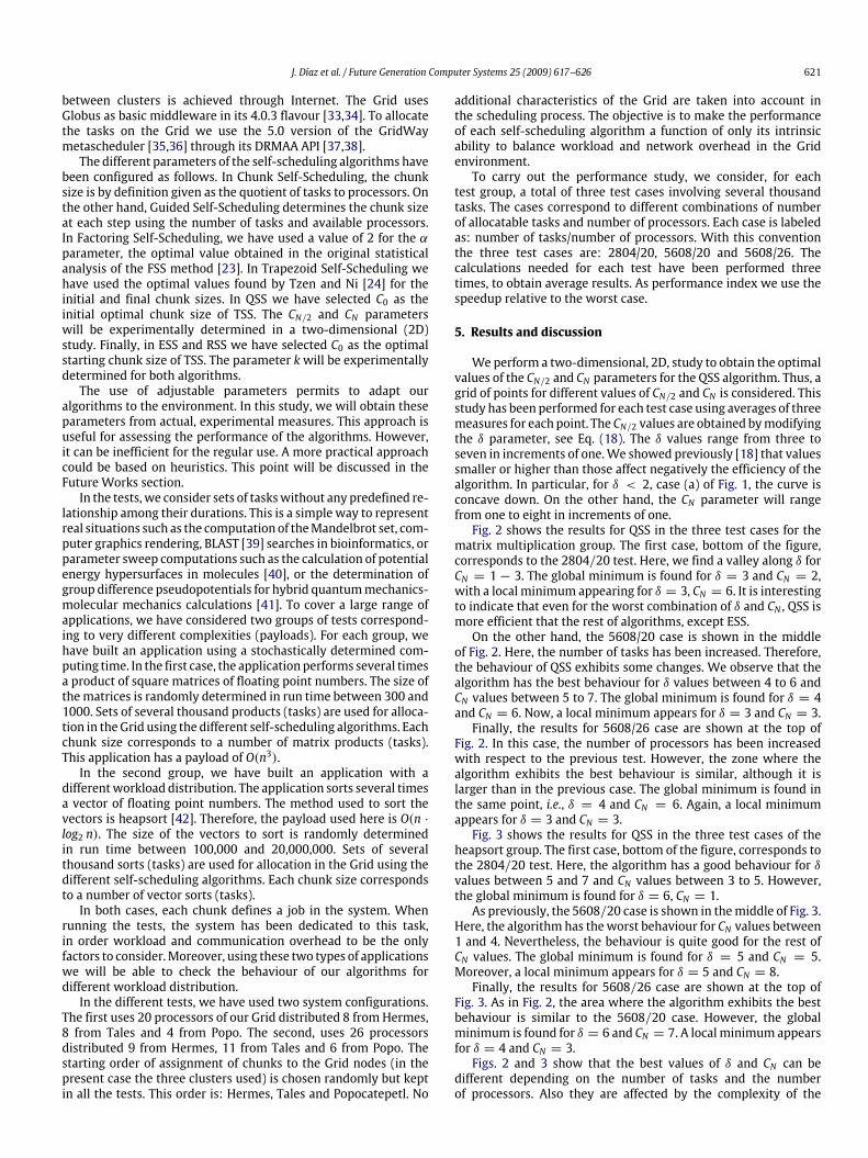
Weperform a two-dimensional, 2D, study to obtain the optimalvalues of the CN/2 and CN parameters for the QSS algorithm. Thus, agrid of points for different values of CN/2 and CN is considered. Thisstudy has been performed for each test case using averages of threemeasures for each point. The CN/2 values are obtained bymodifyingthe δ parameter, see Eq. (18). The δ values range from three toseven in increments of one.We showed previously [18] that valuessmaller or higher than those affect negatively the efficiency of thealgorithm. In particular, for δ < 2, case (a) of Fig. 1, the curve isconcave down. On the other hand, the CN parameter will rangefrom one to eight in increments of one.Fig. 2 shows the results for QSS in the three test cases for the

matrix multiplication group. The first case, bottom of the figure,corresponds to the 2804/20 test. Here, we find a valley along δ forCN = 1 − 3. The global minimum is found for δ = 3 and CN = 2,with a local minimum appearing for δ = 3, CN = 6. It is interestingto indicate that even for the worst combination of δ and CN , QSS ismore efficient that the rest of algorithms, except ESS.On the other hand, the 5608/20 case is shown in the middle

of Fig. 2. Here, the number of tasks has been increased. Therefore,the behaviour of QSS exhibits some changes. We observe that thealgorithm has the best behaviour for δ values between 4 to 6 andCN values between 5 to 7. The global minimum is found for δ = 4and CN = 6. Now, a local minimum appears for δ = 3 and CN = 3.Finally, the results for 5608/26 case are shown at the top of

Fig. 2. In this case, the number of processors has been increasedwith respect to the previous test. However, the zone where thealgorithm exhibits the best behaviour is similar, although it islarger than in the previous case. The global minimum is found inthe same point, i.e., δ = 4 and CN = 6. Again, a local minimumappears for δ = 3 and CN = 3.Fig. 3 shows the results for QSS in the three test cases of the

heapsort group. The first case, bottom of the figure, corresponds tothe 2804/20 test. Here, the algorithm has a good behaviour for δvalues between 5 and 7 and CN values between 3 to 5. However,the global minimum is found for δ = 6, CN = 1.As previously, the 5608/20 case is shown in themiddle of Fig. 3.

Here, the algorithm has theworst behaviour for CN values between1 and 4. Nevertheless, the behaviour is quite good for the rest ofCN values. The global minimum is found for δ = 5 and CN = 5.Moreover, a local minimum appears for δ = 5 and CN = 8.Finally, the results for 5608/26 case are shown at the top of

Fig. 3. As in Fig. 2, the area where the algorithm exhibits the bestbehaviour is similar to the 5608/20 case. However, the globalminimum is found for δ = 6 and CN = 7. A localminimum appearsfor δ = 4 and CN = 3.Figs. 2 and 3 show that the best values of δ and CN can be

different depending on the number of tasks and the numberof processors. Also they are affected by the complexity of the

622 J. Díaz et al. / Future Generation Computer Systems 25 (2009) 617–626

Fig. 2. Matrixmultiplication group: Performance of theQSS algorithmas a functionof δ and CN parameters. Temporal data in seconds. Interval between isocontour lines10 s. Darker zones correspond to lower value zones.

Fig. 3. Heapsort group: Performance of the QSS algorithm as a function of δ andCN parameters. Temporal data in seconds. Interval between isocontour lines 10 s.Darker zones correspond to lower value zones.

processes. In this study, we have selected the best values found foreach case.

Fig. 4. Matrixmultiplication group: Performance of the ESS algorithm as a functionof the k parameter. Temporal data in seconds.

Respect to ESS, the kparameter has been also optimized for eachtest case.We have selected k values ranging from 0.010 to 0.024, inincrements of 0.001. Smaller or larger k values do not provide anysignificant information, since for small k values the exponentialapproaches one, and the chunk size is constant. On the other hand,for large k values the exponential approaches zero, which leadsto very small chunk sizes and, therefore, to a maximization of thecommunication overhead.First, we will consider the tests for the matrix multiplication

group. Fig. 4 represents the performance of the ESS algorithm asa function of the k parameter for the different test cases. Averageof three measures are used for each point. The cases 2804/20and 5608/20 exhibit a similar behaviour. They show a generallynegative slope until k = 0.017,where theminimum is found. Fromhere a generally increasing trend is manifested. The minimumcorresponds to the point where the communication overheadcompensates the load balance in our system. On the other hand,the case 5608/26 has a similar behaviour, with a decreasing trendin the range k = 0.017–0.019. Now the minimum is reached fork = 0.019.On the other hand, Fig. 5 represents the performance of the

ESS algorithm as a function of the k parameter for the differenttest cases in the heapsort group. Here, we observe that, in general,the behaviour of the test cases is similar to that of the matrixmultiplication group. The algorithm exhibits a generally negativeslope until reaching the global minimum for each test case. Testcases 2804/20 and 5608/20 have a similar optimal value of k, thatis 0.023 and 0.024 respectively. However, the minimum for thecase 5608/26 is found in k = 0.019, which is the same value foundin the matrix multiplication group for this test case. From now on,we will use for each test case the corresponding optimal k value.The last algorithm is RSS that depends on a single, k, parameter.

As in ESS, the parameter has been optimized for each test case.Thus, we have selected k values ranging from1 to 41, in incrementsof 2. We consider this interval to be representative of the RSSbehaviour, since smaller or larger k values yield few and longchunks. This fact minimizes the communication overhead, butincreases load imbalance.Fig. 6 represents the working of the RSS algorithm as a

function of the k parameter, in the three test cases of the matrixmultiplication group. Again, averages of three measures are usedfor each point. Here, all cases have a similar behaviour with agenerally increasing trend as k decreases. The minimum is foundfor k = 35.Regarding to the heapsort group, Fig. 7 represents the working

of the RSS algorithm as a function of the k parameter, in thethree test cases. Here, the algorithm has a similar behaviour for alltest cases, but the minimum found is different for each case. The

J. Díaz et al. / Future Generation Computer Systems 25 (2009) 617–626 623

Fig. 5. Heapsort group: Performance of the ESS algorithm as a function of the kparameter. Temporal data in seconds.

Fig. 6. Matrixmultiplication group: Performance of the RSS algorithm as a functionof the k parameter. Temporal data in seconds.

Fig. 7. Heapsort group: Performance of the RSS algorithm as a function of the kparameter. Temporal data in seconds.

minimum found for the 2804/20, 5608/20 and 5608/26 test casescorresponds to k values of 41, 21 and 37, respectively.After calibration of QSS, ESS and RSS, we compare their

performance against the rest of self-scheduling algorithms. Eachalgorithm uses the optimal values of its parameters. The samethree tests are used for each group (matrix and heapsort). Thenumber of chunks allocated in the Grid for the different casesare collected in Table 1. The number of chunks follows the order:

Table 1Number of chunks allocated by the self-scheduling algorithms in the different testcases.

Test case CSS GSS TSS FSS QSS ESS RSS

2804/20 20 108 72 144 84 65 505608/20 20 122 72 168 98 66 425608/26 26 152 95 200 129 175 57

Fig. 8. Matrix multiplication group: Speedup (S), respect to CSS, for the consideredself-scheduling algorithms in the tests performed.

CSS < RSS < ESS < TSS < QSS < GSS < FSS for 20 processorsand CSS < RSS < TSS < QSS < GSS < ESS < FSS for 26processors. The difference arises because of the large increase ofchunks in ESS when the number of processors goes from 20 to26, see Eq. (23). Clearly, in this order the communication overheadincreases.Table 2 collects the time used in the tests (makespan average

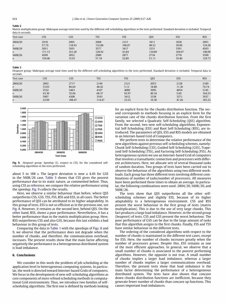
values) of the matrix multiplication group for the differentalgorithms. The standard deviation is also included, σ . Thechanging values of σ , in a range of about 10 to 170 s, reflect thedynamic nature of an actual Grid as the one used here. Anyway,in the worst case (TSS in the 2804/20 test) σ represents just a6.4% of the average time. Table 2 shows that CSS gives the poorestperformance. This is what we can expect due to its static nature(and therefore the lack of adaptability), with a small number oflarge chunks. Thus, using CSS as reference, we compare the relativeperformance using the speedup, here defined as the quotientbetween the time used by CSS and the time used by each algorithm.Fig. 8 collects the speedups so obtained.In all cases, QSS outperforms CSS, GSS, TSS, FSS, RSS and slightly

ESS. The better performance of QSS can be attributed to the higheradaptability of the model (due to its three degrees of freedom)to the heterogeneous environment and conditions used in thetests. It is remarkable than ESS, with only two parameters has asimilar performance to QSS. Therefore, this new algorithm is notonly simple, but seems to be almost as efficient as QSS. On theother hand, RSS, shows a poor perfomance and it only improveswith respect to CSS. Both, RSS and CSS have a similar behaviour,generating a small number of chunks, see Table 1. Despite this, RSSuses a larger number of chunks than CSS, see Table 1, allowing for abetter load balancing. It is interesting to note that RSS correspondsto a concave down curve, see Eq. (25), as the case (a) of QSS, seeEq. (19). Concave down functions for C(t) are translated in a smallnumber of large chunks and therefore they exhibit, as shown herefor RSS and in [18] for QSS, a bad behaviour due to inefficient loadbalancing. Therefore, RSS and the case (a) of QSS show that concavedown functions do not provide good scheduling schemes.On the other hand, we have the heapsort group of tests. In

this case, Table 3 collects the time used in the tests (makespanaverage values) for the different algorithms including the standarddeviation, σ . Here, the dynamic nature of an actual Grid isagain represented by the changing values of σ , in a range of

624 J. Díaz et al. / Future Generation Computer Systems 25 (2009) 617–626

Table 2Matrix multiplication group: Makespan average total time used by the different self-scheduling algorithms in the tests performed. Standard deviation is included. Temporaldata in seconds.

Test case CSS GSS TSS FSS QSS ESS RSS

2804/20 2910 2065 2068 2121 1811 1828 2091σ 57.79 118.93 132.88 106.07 48.52 39.00 124.285608/20 5051 3501 3577 3417 3331 3391 4503σ 171.13 161.28 128.92 41.84 134.89 104.97 148.095608/26 4509 3052 2980 2877 2734 2778 3590σ 150.46 15.01 57.18 22.89 51.11 10.40 129.73

Table 3Heapsort group: Makespan average total time used by the different self-scheduling algorithms in the tests performed. Standard deviation is included. Temporal data inseconds.

Test case CSS GSS TSS FSS QSS ESS RSS

2804/20 2892 2717 2149 2121 2053 2128 2189σ 53.03 86.64 48.42 5.13 18.88 11.36 76.745608/20 5532 5463 4107 4080 3995 4054 5145σ 43.30 35.04 68.37 92.97 40.34 5.69 164.235608/26 5907 4308 3543 3412 3338 3371 3937σ 23.09 188.47 114.47 23.52 19.30 47.26 165.23

Fig. 9. Heapsort group: Speedup (S), respect to CSS, for the considered self-scheduling algorithms in the tests performed.

about 5 to 188 s. The largest deviation is now a 4.4% for GSSin the 5608/26 case. Table 3 shows that CSS gives the poorestperformance due to its static nature, as commented before. Thus,using CSS as reference, we compare the relative performance usingthe speedup. Fig. 9 collects the results.Here, we observe a similar behaviour than before, where QSS

outperforms CSS, GSS, TSS, FSS, RSS and ESS, in all cases. The betterperformance of QSS can be attributed to its higher adaptability. Inthis group of tests, ESS is not so efficient as in the previous one, seeFig. 8. However, it remains as the second best, behind QSS. On theother hand, RSS, shows a poor performance. Nevertheless, it has abetter performance than in the matrix multiplication group. Here,RSS outperforms CSS and also GSS, because this last exhibits a badbehaviour in this group of tests.Comparing the data in Table 1 with the speedups of Figs. 8 and

9, we observe that the performance does not degrade when thenumber of chunks, and therefore, the communication overhead,increases. The present results show that the main factor affectingnegatively the performance in a heterogeneous distributed systemis load imbalance.

6. Conclusions

We consider in this work the problem of job scheduling at theapplication level in heterogeneous computing systems. In particu-lar, thework is directed toward Internet-based Grids of computers.We focus in the development of new self-scheduling algorithms ascore components ofmore refined schedulingmethods in computa-tional Grid environments. Thus, we introduce two families of self-scheduling algorithms. The first one is defined bymethods looking

for an explicit form for the chunks distribution function. The sec-ond corresponds to methods focusing in an explicit form for thevariation rate of the chunks distribution function. From the firstfamily, we selected a Quadratic Self-Scheduling (QSS) algorithm.From the second, two new self-scheduling algorithms, Exponen-tial Self-Scheduling (ESS) and Root Self-Scheduling (RSS), are in-troduced. The parameters of QSS, ESS and RSSmodels are obtainedin an Internet-based Grid of Computers.We perform tests to determine the relative performance of the

newalgorithms against previous self-scheduling schemes, namely:Chunk Self-Scheduling (CSS), Guided Self-Scheduling (GSS), Trape-zoid Self-Scheduling (TSS), and Factoring Self-Scheduling (FSS). Asheterogeneous systemweuse an Internet-basedGrid of computersthat involves a transatlantic connection and processorswith differ-ent architectures. Here, we allocate sets of several thousand tasksof random duration. Two groups of tests have been carried out toobserve the behaviour of the algorithms using two different work-loads. Each group has three different tests involving different com-binations of number of tasks/number of processors. All measureshave been performed three times to obtain an average. In particu-lar, the following combinations were used: 2804/20, 5608/20, and5608/26.The tests show that QSS outperforms all the other self-

scheduling schemes and slightly ESS, because of its higheradaptability to a heterogeneous environment. CSS and RSSpresent the worst behaviour in the first group of tests (matrixmultiplication). This is due to the use of very large chunks. Thisfact produces a large load imbalance. However, in the second group(heapsort) of tests, CSS and GSS present the worst behaviour. Thepoor performance of GSS can be due to the large amount of tasksthat this algorithm assigns to the first chunks. Finally, FSS and TSShave similar behaviour in the different tests.The ordering of the considered algorithms with respect to the

number of chunks is maintained in the different test cases, exceptfor ESS. Here, the number of chunks increases greatly when thenumber of processors grows. Despite this, ESS remains as oneof the most efficient approaches. In general, we observe that asmall number of chunks is associated to the poorest performingalgorithms. However, the opposite is not true. A small numberof chunks implies a larger load imbalance, whereas a largernumber of chunks implies a larger communications overhead.Therefore, the present tests show that load imbalance is themain factor determining the performance of a heterogeneousdistributed system. The tests have also shown that concavedown chunks distribution functions are inefficient, because theygenerate fewer number of chunks than concave up functions. Thiscauses important load imbalances.

J. Díaz et al. / Future Generation Computer Systems 25 (2009) 617–626 625

7. Future works

In the present study, the heterogeneity of the systems isincorporated in the new self-scheduling strategies (QSS andESS) through the calibration of the CN/2, CN and k parameters.Previous works [8,9,11–13,26] have shown that customizationof self-scheduling algorithms in a heterogeneous environment,using the particular characteristics of the processors, greatlyincreases the performance. Mathematically, this is a consequenceof the inclusion of additional degrees of freedom in the model,which makes it more adaptable. Here, QSS and ESS use constantparameters in its definition. This formally corresponds to a parallelsystem where its defining characteristics are constant with time.Therefore, since an actual Grid system is dynamic in nature,we will have a different value of the parameters each time itscharacteristics change. In other words, the most direct solutionto incorporate the dynamic behaviour of an actual Grid systemin our self-scheduling algorithms is to make their parameters afunction of time. One way to achieve this would be to determineheuristically a new set of parameters each time one or severalchunks have been allocated. To such a goal, a direct calibrationin the actual system is clearly impractical. An approach based ina simulation of the system seems much more appropriate.

Acknowledgements

This work has been cofinanced by FEDER funds and theConsejería de Educación y Ciencia de la Junta de Comunidadesde Castilla-La Mancha (grant # PBI08-0008). The Ministerio deEducación y Ciencia (grant # FIS2005-00293) and the Universidadde Castilla-La Mancha are also acknowledged. The authors wishalso to thank the Facultad de CienciasQuímicas and the Laboratoriode Química Teórica of the Universidad Autónoma de Puebla(Mexico), for the use of the Popocatepetl cluster. They alsowish to thank the Distributed Systems Architecture Group ofthe Universidad Complutense de Madrid for their help in theconfiguration and use of GridWay.

References

[1] I. Foster, C. Kesselman, The Grid: Blueprint for a New Computing Infrastruc-ture, Morgan-Kauffman, San Francisco, 1999.

[2] T.L. Casavant, J.G. Kuhl, A taxonomy of scheduling in general-purposedistributed computing, IEEE Transactions on Software Engineering 14 (1988)141–154.

[3] D.J. Lilja, Exploiting the parallelismavailable in loops, IEEE Computer 27 (1994)13–26.

[4] Y. Kee, S. Ha, A robust dynamic load-balancing scheme for data parallelapplication on message passing architecture, in: Int. Conf. on Parallel andDistributed Processing Techniques and Applications, 1998, pp. 974–980.

[5] C. Yang, S. Chang, A parallel loop self-scheduling on extremely heterogeneousPC clusters, Journal of Information Science and Engineering 20 (2004)263–273.

[6] T. Philip, C.R. Das, Evaluation of loop scheduling algorithms on distributedmemory systems, in: Proc. of Int. Conf. on Parallel and Distributed ComputingSystems, 1997.

[7] T.H. Kim, J.M. Purtilo, Load balancing for parallel loops in workstation clusters,in: Proc. of Int. Conf. on Parallel Processing, 1996, pp. 182–189.

[8] B. Hamidzadeh, D.J. Lilja, Y. Atif, Dynamic scheduling techniques forheterogeneous computing systems, Concurrency: Practice and Experience 7(1995) 633–652.

[9] F. Berman, R. Wolski, S. Figueira, J. Schopf, G. Shao, Application-level schedul-ing on distributed heterogeneous networks, in: Proc. of Supercomputing ’96,1996, p. 39.

[10] F. Berman, High-performance schedulers, in: I. Foster, C. Kesselman (Eds.), TheGrid: Blueprint for a New Computing Infrastructure, Morgan-Kaufmann, SanFrancisco, 1999, pp. 279–309.

[11] A.T. Chronopoulos, M. Benche, D. Grosu, R. Andonie, A class of loop self-scheduling for heterogeneous clusters, in: Proc. of the 2001 IEEE Int. Conf. onCluster Computing, 2001, pp. 282–294.

[12] A.T. Chronopoulos, S. Penmatsa, N. Yu, Scalable loop self-scheduling schemesfor heterogeneous clusters, in: Proc. 2002 IEEE Int. Conf. on Cluster Computing,2002, pp. 353–359.

[13] A.T. Chronopoulos, S. Penmatsa, J. Xu, S. Ali, Distributed loop schedulingschemes for heterogeneous computer systems, Concurrency: Practice andExperience 18 (2006) 771–785.

[14] J. Díaz, S. Reyes, A. Niño, C. Muñoz-Caro, Un Algoritmo AutoplanificadorCuadrático para Clusters Heterogéneos de Computadores, in: XVII Jornadas deParalelismo, 2006, pp. 379–382.

[15] P.J. Sokolowski, D. Grosu, C. Xu, Analysis of performance behaviors of Gridconnected clusters, in: M. Ould-khaoua, G. Min (Eds.), Performance Evaluationof Parallel and Distributed Systems, Nova Science, New York, 2006.

[16] J. Herrera, E. Huedo, R.S. Montero, I.M. Llorente, Ejecución Distribuida deBucles en Grids Computacionales, in: 3a Reunión para la Red Temática en GridMiddleware, 2005.

[17] S. Penmatsa, A.T. Chronopoulos, N.T. Karonis, B. Toonen, Implementation ofdistributed loop scheduling schemes on the TeraGrid, in: Proc. of the 21stIEEE Int. Parallel and Distributed Processing Symp. (IPDPS 2007), 4th HighPerformance Grid Computing Workshop, 2007, pp. 1–8.

[18] J. Díaz, S. Reyes, A. Niño, C. Muñoz-Caro, A quadratic self-scheduling algorithmfor heterogeneous distributed computing systems, in: Proc. of the 5th Int.Workshop on Algorithms, Models and Tools for Parallel Computing onHeterogeneous Networks, HeteroPar ’06, 2006, pp. 1–8.

[19] J. Díaz, S. Reyes, A. Niño, C. Muñoz-Caro, New self-scheduling schemesfor internet-based Grids of computers, in: 1st Iberian Grid InfrastructureConference, IBERGRID, 2007, pp. 184–195.

[20] C.P. Kruskal, A. Weiss, Allocating independent subtasks on parallel processors,IEEE Transactions on Software Engineering 11 (1985) 1001–1016.

[21] P. Tang, P.C. Yew, Processor self-scheduling for multiple nested parallel loops,in: Proc. of the 1986 Int. Conf. on Parallel Processing, 1986, pp. 528–535.

[22] C.D. Polychronopoulos, D. Kuck, Guided self-scheduling: Apractical schedulingscheme for parallel supercomputers, IEEE Transactions on Computers 36(1987) 1425–1439.

[23] S.F. Hummel, E. Schonberg, L.E. Flynn, Factoring: A method for schedulingparallel loops, Communications of the ACM 35 (1992) 90–101.

[24] T.H. Tzen, L.M. Ni, Trapezoid self-scheduling: A practical scheduling schemefor parallel compilers, IEEE Transactions on Parallel and Distributed Systems 4(1993) 87–98.

[25] E.P. Markatos, T.J. LeBlanc, Using processor affinity in loop schedulingon shared-memory multiprocessors, IEEE Transactions on Parallel andDistributed Systems 5 (1994) 379–400.

[26] S.F. Hummel, J. Schmidt, R.N. Uma, J. Wein, Load-sharing in heterogeneoussystems via weighted factoring, in: Proc. of the 8th Annu. ACM Symp. onParallel Algorithms and Architectures, 1996, pp. 318–328.

[27] I. Banicescu, Z. Liu, Adaptive factoring: A dynamic scheduling method tunedto the rate of weight changes, in: Proc. of the High Performance ComputingSymp., 2000, pp. 122–129.

[28] F.M. Ciorba, T. Andronikos, I. Riakiotakis, A.T. Chronopoulos, G. Papakonstanti-nou, Dynamic multi phase scheduling for heterogeneous clusters, in: Proc. ofthe 20th IEEE Int. Parallel & Distributed Processing Symp., IPDPS 2006, 2006,p. 10.

[29] I. Riakiotakis, F.M. Ciorba, T. Andronikos, G. Papakonstantinou, Self-adaptingscheduling for taskswith dependencies in stochastic environments, in: Proc. ofthe 5th Int.Workshop on Algorithms,Models and Tools for Parallel Computingon Heterogeneous Networks, HeteroPar ’06, 2006, p. 1–8.

[30] A. Kejariwal, A. Nicolau, C.D. Polychronopoulos, An efficient approach for self-scheduling parallel loops on multiprogrammed parallel computers, in: The18th Int.Workshop on Languages and Compilers for Parallel Computing, LCPC,2005, pp. 441–449.

[31] S.P. Dandamudi, T.K. Thyagaraj, A hierarchical processor scheduling policy fordistributed-memory multicompute system, in: Proc. 4th Int. Conf. on HighPerformance Computing, 1997, pp. 218–223.

[32] T.M. Apostol, Calculus, second ed., Reverté, Barcelona, Spain, 1998.[33] I. Foster, Globus toolkit version 4: Software for service-oriented systems,

in: IFIP Int. Conf. on Network and Parallel Computing, in: LNCS, vol. 3779,Springer-Verlag, 2005, pp. 2–13.

[34] I. Foster, C. Kesselman, The globus project: A status report, Future GenerationComputer Systems 15 (1999) 607–621.

[35] E. Huedo, R.S. Montero, I.M. Llorente, Amodular meta-scheduling architecturefor interfacing with pre-WS and WS Grid resource management services,Future Generation Computer Systems 23 (2007) 252–261.

[36] R.S. Montero, E. Huedo, I.M. Llorente, The GridWay approach for jobsubmission and management on Grids, in: iAstro Workshop on DistributedProcessing, Transfer, Retrieval, Fusion and Display of Images and Signals: HighResolution and Low Resolution in Data and Information Grids, 2003.

[37] Distributed resourcemanagement application api working group— The globalGrid forum. http://www.drmaa.org (last access December 2008).

[38] Open Grid forum. http://www.ogf.org (last access December 2008).[39] S.F. Altschul, W. Gish,W. Miller, E.W. Myers, D.J. Lipman, Basic local alignment

search tool, Journal of Molecular Biology 215 (1990) 403–410.[40] S. Reyes, C. Muñoz-Caro, A. Niño, R.M. Badia, J.M. Cela, Performance of

computationally intensive parameter sweep applications on internet-basedGrids of computers: Themapping ofmolecular potential energyhypersurfaces,Concurrency: Practice and Experience 19 (2007) 463–481.

[41] W. Sudholt, K.K. Balgridge, Parameter scan of an effective group differencepseudopotencial usingGrid computing, Grid System for Life Sciences 22 (2003)137–146.

[42] D. Knuth, TheArt of Computer Programming, Volume3: Sorting and Searching,second ed., Addison-Wesley, California, 1997.

626 J. Díaz et al. / Future Generation Computer Systems 25 (2009) 617–626

Javier Díaz received theM.Sc. degree in Computer Sciencefrom the Castilla-La Mancha University, Spain, in 2005.Actually, he is a Ph.D. candidate in the Castilla-La ManchaUniversity (UCLM). His research interests are in the areasof computational grids and scheduling algorithms.

Sebastián Reyes is Computer Science Engineer from theGranada University, Spain. He is currently a member ofthe Department of Information Technologies and Systemsat the Castilla-La Mancha University (UCLM), Spain. Heis a lecturer in Computer Networks. His present researchinterests are in clustering and Grid computing.

Alfonso Niño received his Ph.D. degree from the Com-plutenseUniversity inMadrid, Spain. Hismultidisciplinarywork involves Computer Science and Molecular Physics.Formerly, he worked at the National Research Council ofSpain (CSIC) and is currently a member of the Departmentof Information Technologies and Systems at the Castilla-La Mancha University (UCLM), Spain. He has been a lec-turer in Theoretical Chemistry, Software Engineering andObject Oriented Programming. His research interests arein the fields of clustering and Grid computing applied toScientific Computing.

Camelia Muñoz-Caro received her Ph.D. degree from theComplutense University inMadrid, Spain. Herwork coversComputer Science and Molecular Physics. Formerly, sheworked at the National Research Council of Spain (CSIC),being currently a member of the Department of Informa-tion Technologies and Systems at the Castilla-La ManchaUniversity (UCLM), Spain. She has been a lecturer in Theo-retical Chemistry, Management Information Systems andObject Oriented Programming. Her research interests arein the fields of clustering and Grid computing applied toScientific Computing.