Derivation of an EM algorithm for constrained and …€¦ · · 2018-04-14Derivation of an EM...

Derivation of an EM algorithm for constrained and unconstrained

multivariate autoregressive state-space (MARSS) models

Elizabeth Eli Holmes*

March 30, 2018

Abstract

This report presents an Expectation-Maximization (EM) algorithm for estimation of the maximum-likelihood parameter values of constrained multivariate autoregressive Gaussian state-space (MARSS)models. The MARSS model can be written: x(t)=Bx(t-1)+u+w(t), y(t)=Zx(t)+a+v(t), where w(t) andv(t) are multivariate normal error-terms with variance-covariance matrices Q and R respectively. MARSSmodels are a class of dynamic linear model and vector autoregressive model state-space model. Shumwayand Stoffer presented an unconstrained EM algorithm for this class of models in 1982, and a number ofresearchers have presented EM algorithms for specific types of constrained MARSS models since then. Inthis report, I present a general EM algorithm for constrained MARSS models, where the constraints are onthe elements within the parameter matrices (B,u,Q,Z,a,R). The constraints take the form vec(M)=f+Dm,where M is the parameter matrix, f is a column vector of fixed values, D is a matrix of multipliers, andm is the column vector of estimated values. This allows a wide variety of constrained parameter matrixforms. The presentation is for a time-varying MARSS model, where time-variation enters through thefixed (meaning not estimated) f(t) and D(t) matrices for each parameter. The algorithm allows missingvalues in y and partially deterministic systems where 0s appear on the diagonals of Q or R.

Keywords: Time-series analysis, Kalman filter, EM algorithm, maximum-likelihood, vector autoregressivemodel, dynamic linear model, parameter estimation, state-space

citation: Holmes, E. E. 2012. Derivation of an EM algorithm for constrained and unconstrained multivariate autoregressive state-space (MARSS) models.

*Northwest Fisheries Science Center, NOAA Fisheries, Seattle, WA 98112, [email protected],http://faculty.washington.edu/eeholmes

1

1 Overview

EM algorithms extend maximum-likelihood estimation to models with hidden states and are widely used inengineering and computer science applications. This report presents an EM algorithm for a general class ofGaussian constrained multivariate autoregressive state-space (MARSS) models, with a hidden multivariateautoregressive process (state) model and a multivariate observation model. This is an important class oftime-series model used in many different scientific fields. The reader is referred to McLachlan and Krishnan(2008) for general background on EM algorithms and to Harvey (1989) for a discussion of EM algorithms fortime-series data. Borman (2009) has a nice tutorial on the EM algorithm.

Before showing the derivation for the constrained case, I first show a derivation of the EM algorithm forunconstrained1 MARSS model. This EM algorithm was published by Shumway and Stoffer (1982), but myderivation is more similar to Ghahramani et al’s (Ghahramani and Hinton, 1996; Roweis and Ghahramani,1999) slightly different presentation. One difference in my presentation and all these previous presentations,however, is that I treat the data as a random variable throughout; this means that there are no “special”update equations for the missing values case. Another difference is that I present the update equations forboth stochastic initial states and fixed initial states. I then extend the derivation to constrained MARSSmodels where there are fixed and shared elements in the parameter matrices and to the case of degenerateMARSS models where some processes in the model are deterministic rather than stochastic. See also Wuet al. (1996) and Zuur et al. (2003) for other examples of the EM algorithm for different classes of constrainedMARSS models.

When working with MARSS models, one should be cognizant that misspecification of the prior on theinitial hidden states can have catastrophic and difficult to detect effects on the parameter estimates. There isoften no sign that something is amiss with the MLE estimates output by an EM algorithm. There has beenmuch work on how to avoid these initial conditions effects; see especially literature on vector autoregressivestate-space models in the economics literature. The trouble often occurs when the prior on the initial statesis inconsistent with the distribution of the initial states that is implied by the maximum-likelihood model.This often happens when the model implies a specific covariance structure on the initial states, but sincethe maximum-likelihood parameters are unknown, this covariance structure is unknown. Using a diffuseprior does not help since your diffuse prior still has some covariance structure (often independence is beingimposed). In some ways the EM algorithm is less sensitive to a misspecified prior because it uses the smoothedstates conditioned on all the data. However, if the prior is inconsistent with the model, the EM algorithmwill not (cannot) find the MLEs. It is very possible however that it will find parameter estimates that arecloser to what you intend (estimates uninfluenced by the prior), but they will not be MLEs. The derivationpresented here allows one to circumvent these problems by treating the initial states as fixed (and estimated)parameters. The problematic initial state variance-covariance matrix is removed from the model, albeit atthe cost of additional estimated parameters.

Finally, when working with MARSS models, one needs to ensure that the model is identifiable, i.e. aunique solution exists. For a given MARSS model, some of the parameter elements will need to be fixed (notestimated) in order to produce a model with one solution. How to do that depends on the MARSS modelbeing fitted and is up to the user.

1.1 The MARSS model

The linear MARSS model with a stochastic initial state2 is

xxxt = Bxxxt−1 + u + wt, where Wt ∼ MVN(0,Q) (1a)

yyyt = Zxxxt + a + vt, where Vt ∼ MVN(0,R) (1b)

XXX0 ∼ MVN(ξ,Λ) (1c)

The yyy equation is called the observation process, and yyyt is a n× 1 vector. The xxx equation is called the stateor process equation, and xxxt is a m × 1 vector. The equation for xxx describes a multivariate autoregressiveprocess (also called a random walk or Markov process). w are the process errors and are specific realizationsof the random variable W; v is defined similarly. The initial state can either defined at t = 0, as is done in

1“unconstrained” means that each element in the parameter matrix is estimated and no elements are fixed or shared.2‘Stochastic’ means the initial state has a distribution rather than a fixed value. Because the process must start somewhere,

one needs to specify the initial state. In equation 1, I show the initial state specified as a distribution. However, the derivationwill also discuss the case where the initial state is specified as an unknown fixed parameter.

2

equation 1, or at t = 1. When presenting the MARSS model, I use t = 0 but the derivations will show theEM algorithm for both cases. Q and R are variance-covariance matrices that specify the stochasticity in theobservation and state equations.

In the MARSS model, xxx and yyy equations describe two stochastic processes. By tradition, one conditionson observations of yyy, and xxx is treated as completely hidden, hence the name ‘hidden Markov process’ of whicha MARSS model is a special type. However, you could condition on (partial) observations of xxx and treat yyyas a (partially) hidden process—with as usual proper constraints to ensure identifiability. Nonetheless in thisreport, I follow tradition and treat xxx as hidden and yyy as (partially) observed. If xxx is partially observed thenthe update equations stay the same but the expectations shown in section 6 would be computed conditionedon the partially observed xxx.

The first part of this report will review the derivation of an EM algorithm for the time-constant MARSSmodel (equation 1). However the main objective of this report is to show the derivation of an EM algorithmto solve a much more general MARSS model (section 4), which is a MARSS model with linear constraintson time-varying parameters:

xxxt = Btxxxt−1 + ut + Gtwt, where Wt ∼ MVN(0,Qt)

yyyt = Ztxxxt + at + Htvt, where Vt ∼ MVN(0,Rt)

xxxt0 = ξ + Fl, where l ∼ MVN(0,Λ)

(2)

The linear constraints appear as the vectorization of each parameter (B, u, Q, Z, a, R, ξ, Λ) is describedby the relation f t + Dtm. This relation specifies linear constraints of the form βi + βa,ia + βb,ib + . . . onthe elements in each MARSS parameter matrix. Equation (2) is a much broader class of MARSS modelsthat includes MARSS models with exogenous variable (covariates), AR-p models, moving average models,constrained MARSS models and models that are combinations of these. The derivation also includes partiallydeterministic systems where Gt, Ht and F may have all zero rows.

1.2 The joint log-likelihood function

Equation 2 describes a multivariate stochastic process and YYY t and XXXt are random variables whose distri-butions are given by Equation 2. Denote a specific realization of these random variables as yyy and xxx whichdenotes a set of all y’s and x’s from t = 1 to T . The joint log-likelihood3 of yyy and xxx can then be written thenas follows4, where XXXt denotes the random variable and xxxt is a realization from that random variable (andsimilarly for YYY t):

5

f(yyy,xxx) = f(yyy|XXX = xxx)f(xxx), (3)

where

f(xxx) = f(xxx0)

T∏t=1

f(xxxt|XXXt−11 = xxxt−1

1 )

f(yyy|XXX = xxx) =

T∏t=1

f(yyyt|XXX = xxx)

(4)

Thus,

f(yyy,xxx) =

T∏t=1

f(yyyt|XXX = xxx)× f(xxx0)

T∏t=1

f(xxxt|XXXt−11 = xxxt−1

1 )

=

T∏t=1

f(yyyt|XXXt = xxxt)× f(xxx0)

T∏t=1

f(xxxt|XXXt−1 = xxxt−1).

(5)

Here xxxt2t1 denotes the set of xxxt from t = t1 to t = t2 (and thus xxx is shorthand for xxxT1 ). The third line followsbecause conditioned on xxx, the yyyt’s are independent of each other (because the vt are independent of each

3This is not the log likelihood output by the Kalman filter. The log likelihood output by the Kalman filter is the logL(yyy; Θ)(notice xxx does not appear), which is known as the marginal log likelihood.

4The log-likelihood function is shown here for the MARSS with non-time varying parameters (equation 1).5To alleviate clutter, I have left off subscripts on the f ’s. To emphasize that the f ’s represent different density functions, one

would often use a subscript showing what parameters are in the functions, i.e. f(xxxt|XXXt−1 = xxxt−1) becomes fB,u,Q(xxxt|XXXt−1 =xxxt−1).

3

other). In the last line, xxxt−11 becomes xxxt−1 from the Markov property of the equation for xxxt (equation 1a),

and xxx becomes xxxt because yyyt depends only on xxxt (equation 1b).Since (XXXt|XXXt−1 = xxxt−1) is multivariate normal and (YYY t|XXXt = xxxt) is multivariate normal (equation 1),

we can write down the joint log-likelihood function using the likelihood function for a multivariate normaldistribution (Johnson and Wichern, 2007, sec. 4.3).

log L(yyy,xxx; Θ) = −T∑1

1

2(yyyt − Zxxxt − a)>R−1(yyyt − Zxxxt − a)−

T∑1

1

2log |R|

−T∑1

1

2(xxxt −Bxxxt−1 − u)>Q−1(xxxt −Bxxxt−1 − u)−

T∑1

1

2log |Q|

− 1

2(xxx0 − ξ)>Λ−1(xxx0 − ξ)− 1

2log |Λ| − n

2log 2π

(6)

n is the number of data points. This is the same as equation 6.64 in Shumway and Stoffer (2006). The aboveequation is for the case where xxx0 is stochastic (has a known distribution). However, if we instead treat xxx0 asfixed but unknown (section 3.4.4 in Harvey, 1989), it is then a parameter and there is no Λ. The likelihoodthen is slightly different. xxx0 is defined as a parameter ξ and


1


T∑1

1

2log |R|

−T∑1

1


T∑1

1

2log |Q|

(7)

Note that in this case, xxx0 is no longer a realization of a random variable XXX0; it is a fixed (but unknown)parameter. Equation 7 is written as if all the xxx0 are fixed, however when the general derivation is presented,it allowed that some xxx0 are fixed (Λ=0) and others are stochastic.

If R is constant through time, then∑T

112 log |R| in the likelihood equation reduces to T

2 log |R|, however

sometimes one needs to includes time-dependent weighting on R6. The same applies to∑T

112 log |Q|.

All bolded elements are column vectors (lower case) and matrices (upper case). A> is the transpose ofmatrix A, A−1 is the inverse of A, and |A| is the determinant of A. Parameters are non-italic while elementsthat are slanted are realizations of a random variable (xxx and yyy are slated)7

1.3 Missing values

In Shumway and Stoffer and other presentations of the EM algorithm for MARSS models (Shumway andStoffer, 2006; Zuur et al., 2003), the missing values case is treated separately from the non-missing valuescase. In these derivations, a series of modifications are given for the EM update equations when there aremissing values. In my derivation, I present the missing values treatment differently, and there is only one setof update equations and these equations apply in both the missing values and non-missing values cases. Myderivation does this by keeping E[YYY t|data] and E[YYY tXXX

>t |data] in the update equations (much like E[XXXt|data]

is kept in the equations) while Shumway and Stoffer replace these expectations involving YYY t by their values,which depend on whether or not the data are a complete observation of YYY t with no missing values. Section6 shows how to compute the expectations involving YYY t when the data are an incomplete observation of YYY t.

6If for example, one wanted to include a temporally dependent weighting on R replace |R| with |αtR| = αnt |R|, where αt

is the weighting at time t and is fixed not estimated.7In matrix algebra, a capitol bolded letter indicates a matrix. Unfortunately in statistics, the capitol letter convention is

used for random variables. Fortunately, this derivation does not need to reference random variables except indirectly when usingexpectations. Thus, I use capitols to refer to matrices not random variables. The one exception is the reference to XXX and YYY . Inthis case a bolded slanted capitol is used.

4

2 The EM algorithm

The EM algorithm cycles iteratively between an expectation step (the integration in the equation) followedby a maximization step (the arg max in the equation):

Θj+1 = arg maxΘ

∫xxx

∫yyy

log L(xxx,yyy; Θ)f(xxx,yyy|YYY (1) = yyy(1),Θj)dxxxdyyy (8)

YYY (1) indicates those YYY that have an observation and yyy(1) are the actual observations. Note that Θ andΘj are different. If Θ consists of multiple parameters, we can also break this down into smaller steps. LetΘ = α, β, then

αj+1 = arg maxα

∫xxx

∫yyy

log L(xxx,yyy, βj ;α)f(xxx,yyy|YYY (1) = yyy(1), αj , βj)dxxxdyyy (9)

Now the maximization is only over α, the part that appears after the “;” in the log-likelihood.Expectation step The integral that appears in equation (8) is an expectation. The first step in the EM

algorithm is to compute this expectation. This will involve computing expectations like E[XXXtXXX>t |YYY t(1) =

yyyt(1),Θj ] and E[YYY tXXX>t |YYY t(1) = yyyt(1),Θj ]. The j subscript on Θ denotes that these are the parameters at

iteration j of the algorithm.Maximization step: A new parameter set Θj+1 is computed by finding the parameters that maximize

the expected log-likelihood function (the part in the integral) with respect to Θ. The equations that give theparameters for the next iteration (j + 1) are called the update equations and this report is devoted to thederivation of these update equations.

After one iteration of the expectation and maximization steps, the cycle is then repeated. New expecta-tions are computed using Θj+1, and then a new set of parameters Θj+2 is generated. This cycle is continueduntil the likelihood no longer increases more than a specified tolerance level. This algorithm is guaranteed toincrease in likelihood at each iteration (if it does not, it means there is an error in one’s update equations).The algorithm must be started from an initial set of parameter values Θ1. The algorithm is not particularlysensitive to the initial conditions but the surface could definitely be multi-modal and have local maxima. Seesection 11 on using Monte Carlo initialization to ensure that the global maximum is found.

2.1 The expected log-likelihood function

The function that is maximized in the “M” step is the expected value of the log-likelihood function. Thisexpectation is conditioned on two things: 1) the observed YYY ’s which are denoted YYY (1) and which are equal tothe fixed values yyy(1) and 2) the parameter set Θj . Note that since there may be missing values in the data,YYY (1) can be a subset of YYY , that is, only some YYY have a corresponding yyy value at time t. Mathematically whatwe are doing is EXY[g(XXX,YYY )|YYY (1) = yyy(1),Θj ]. This is a multivariate conditional expectation becauseXXX,YYY ismultivariate (a m×n×T vector). The function g(Θ) that we are taking the expectation of is log L(YYY ,XXX; Θ).Note that g(Θ) is a random variable involving the random variables, XXX and YYY , while log L(yyy,xxx; Θ) is not arandom variable but rather a specific value since yyy and xxx are a set of specific values.

We denote this expected log-likelihood by Ψ. The goal is to find the Θ that maximize Ψ and this becomesthe new Θ for the j + 1 iteration of the EM algorithm. The equations to compute the new Θ are termed theupdate equations. Using the log likelihood equation (6) and expanding out all the terms, we can write out

5

Ψ in verbose form as:

EXY[log L(YYY ,XXX; Θ);YYY (1) = yyy(1),Θj ] = Ψ =

− 1

2

T∑1

(E[YYY >t R−1YYY t]− E[YYY >t R−1ZXXXt]− E[(ZXXXt)

>R−1YYY t]− E[a>R−1YYY t]− E[YYY >t R−1a]

+ E[(ZXXXt)>R−1ZXXXt] + E[a>R−1ZXXXt] + E[(ZXXXt)

>R−1a] + E[a>R−1a]

)− T

2log |R|

− 1

2

T∑1

(E[XXX>t Q−1XXXt]− E[XXX>t Q−1BXXXt−1]− E[(BXXXt−1)>Q−1XXXt]

− E[u>Q−1XXXt]− E[XXX>t Q−1u] + E[(BXXXt−1)>Q−1BXXXt−1]

+ E[u>Q−1BXXXt−1] + E[(BXXXt−1)>Q−1u] + u>Q−1u

)− T

2log |Q|

− 1

2

(E[XXX>0 V−1

0 XXX0]− E[ξ>Λ−1XXX0]− E[XXX>0 Λ−1ξ] + ξ>Λ−1ξ

)− 1

2log |Λ| − n

2log π

(10)

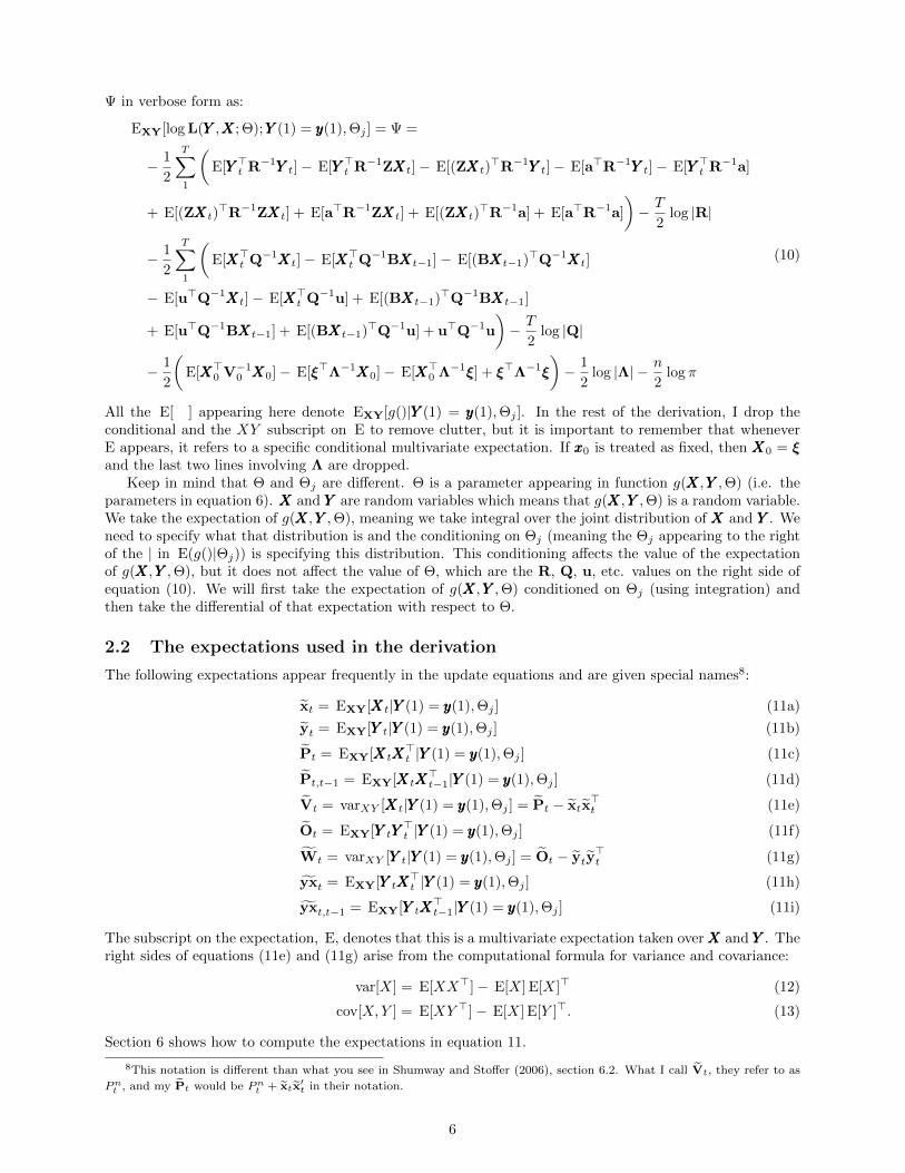
All the E[ ] appearing here denote EXY[g()|YYY (1) = yyy(1),Θj ]. In the rest of the derivation, I drop theconditional and the XY subscript on E to remove clutter, but it is important to remember that wheneverE appears, it refers to a specific conditional multivariate expectation. If xxx0 is treated as fixed, then XXX0 = ξand the last two lines involving Λ are dropped.

Keep in mind that Θ and Θj are different. Θ is a parameter appearing in function g(XXX,YYY ,Θ) (i.e. theparameters in equation 6). XXX and YYY are random variables which means that g(XXX,YYY ,Θ) is a random variable.We take the expectation of g(XXX,YYY ,Θ), meaning we take integral over the joint distribution of XXX and YYY . Weneed to specify what that distribution is and the conditioning on Θj (meaning the Θj appearing to the rightof the | in E(g()|Θj)) is specifying this distribution. This conditioning affects the value of the expectationof g(XXX,YYY ,Θ), but it does not affect the value of Θ, which are the R, Q, u, etc. values on the right side ofequation (10). We will first take the expectation of g(XXX,YYY ,Θ) conditioned on Θj (using integration) andthen take the differential of that expectation with respect to Θ.

2.2 The expectations used in the derivation

The following expectations appear frequently in the update equations and are given special names8:

xt = EXY[XXXt|YYY (1) = yyy(1),Θj ] (11a)

yt = EXY[YYY t|YYY (1) = yyy(1),Θj ] (11b)

Pt = EXY[XXXtXXX>t |YYY (1) = yyy(1),Θj ] (11c)

Pt,t−1 = EXY[XXXtXXX>t−1|YYY (1) = yyy(1),Θj ] (11d)

Vt = varXY [XXXt|YYY (1) = yyy(1),Θj ] = Pt − xtx>t (11e)

Ot = EXY[YYY tYYY>t |YYY (1) = yyy(1),Θj ] (11f)

Wt = varXY [YYY t|YYY (1) = yyy(1),Θj ] = Ot − yty>t (11g)

yxt = EXY[YYY tXXX>t |YYY (1) = yyy(1),Θj ] (11h)

yxt,t−1 = EXY[YYY tXXX>t−1|YYY (1) = yyy(1),Θj ] (11i)

The subscript on the expectation, E, denotes that this is a multivariate expectation taken overXXX and YYY . Theright sides of equations (11e) and (11g) arise from the computational formula for variance and covariance:

var[X] = E[XX>]− E[X] E[X]> (12)

cov[X,Y ] = E[XY >]− E[X] E[Y ]>. (13)

Section 6 shows how to compute the expectations in equation 11.

8This notation is different than what you see in Shumway and Stoffer (2006), section 6.2. What I call Vt, they refer to as

Pnt , and my Pt would be Pn

t + xtx′t in their notation.

6

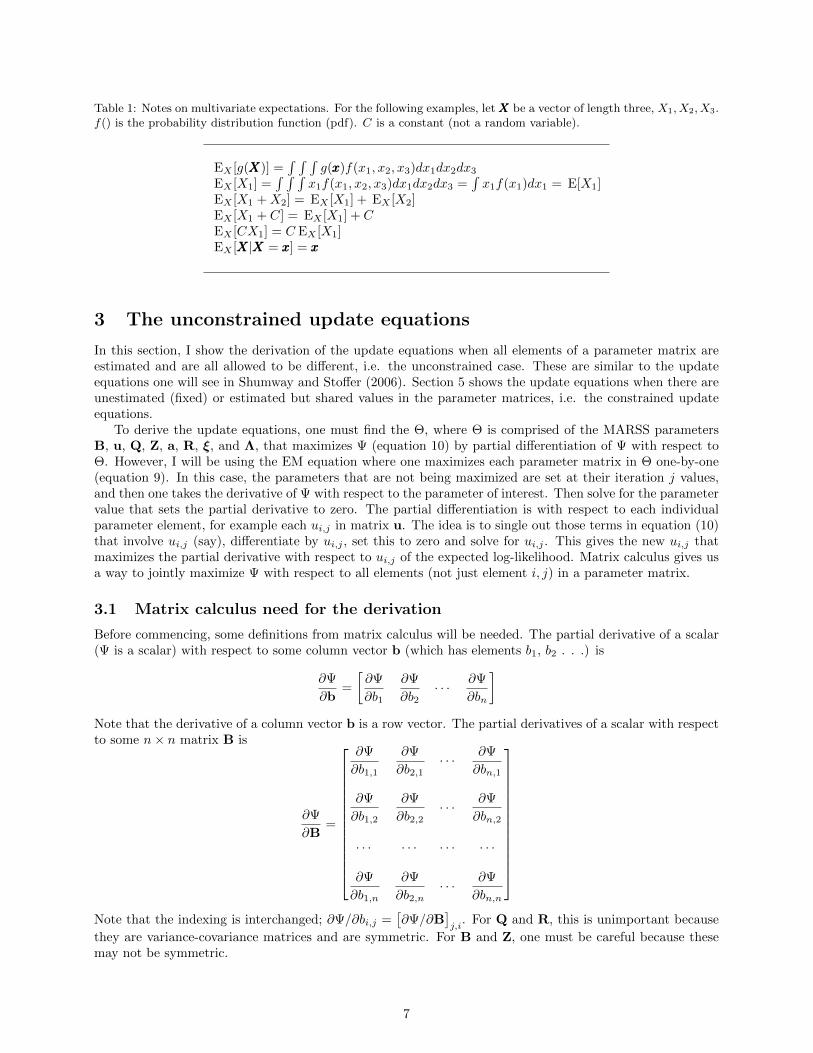
Table 1: Notes on multivariate expectations. For the following examples, let XXX be a vector of length three, X1, X2, X3.f() is the probability distribution function (pdf). C is a constant (not a random variable).

EX [g(XXX)] =∫ ∫ ∫

g(xxx)f(x1, x2, x3)dx1dx2dx3

EX [X1] =∫ ∫ ∫

x1f(x1, x2, x3)dx1dx2dx3 =∫x1f(x1)dx1 = E[X1]

EX [X1 +X2] = EX [X1] + EX [X2]EX [X1 + C] = EX [X1] + CEX [CX1] = C EX [X1]EX [XXX|XXX = xxx] = xxx

3 The unconstrained update equations

In this section, I show the derivation of the update equations when all elements of a parameter matrix areestimated and are all allowed to be different, i.e. the unconstrained case. These are similar to the updateequations one will see in Shumway and Stoffer (2006). Section 5 shows the update equations when there areunestimated (fixed) or estimated but shared values in the parameter matrices, i.e. the constrained updateequations.

To derive the update equations, one must find the Θ, where Θ is comprised of the MARSS parametersB, u, Q, Z, a, R, ξ, and Λ, that maximizes Ψ (equation 10) by partial differentiation of Ψ with respect toΘ. However, I will be using the EM equation where one maximizes each parameter matrix in Θ one-by-one(equation 9). In this case, the parameters that are not being maximized are set at their iteration j values,and then one takes the derivative of Ψ with respect to the parameter of interest. Then solve for the parametervalue that sets the partial derivative to zero. The partial differentiation is with respect to each individualparameter element, for example each ui,j in matrix u. The idea is to single out those terms in equation (10)that involve ui,j (say), differentiate by ui,j , set this to zero and solve for ui,j . This gives the new ui,j thatmaximizes the partial derivative with respect to ui,j of the expected log-likelihood. Matrix calculus gives usa way to jointly maximize Ψ with respect to all elements (not just element i, j) in a parameter matrix.

3.1 Matrix calculus need for the derivation

Before commencing, some definitions from matrix calculus will be needed. The partial derivative of a scalar(Ψ is a scalar) with respect to some column vector b (which has elements b1, b2 . . .) is

∂Ψ

∂b=

[∂Ψ

∂b1

∂Ψ

∂b2· · · ∂Ψ

∂bn

]Note that the derivative of a column vector b is a row vector. The partial derivatives of a scalar with respectto some n× n matrix B is

∂Ψ

∂B=

∂Ψ

∂b1,1

∂Ψ

∂b2,1· · · ∂Ψ

∂bn,1

∂Ψ

∂b1,2

∂Ψ

∂b2,2· · · ∂Ψ

∂bn,2

· · · · · · · · · · · ·

∂Ψ

∂b1,n

∂Ψ

∂b2,n· · · ∂Ψ

∂bn,n

Note that the indexing is interchanged; ∂Ψ/∂bi,j =

[∂Ψ/∂B

]j,i

. For Q and R, this is unimportant because

they are variance-covariance matrices and are symmetric. For B and Z, one must be careful because thesemay not be symmetric.

7

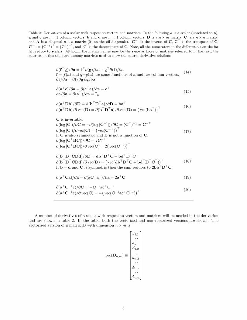
Table 2: Derivatives of a scalar with respect to vectors and matrices. In the following a is a scalar (unrelated to a),a and c are n × 1 column vectors, b and d are m × 1 column vectors, D is a n ×m matrix, C is a n × n matrix,and A is a diagonal n × n matrix (0s on the off-diagonals). C−1 is the inverse of C, C> is the transpose of C,

C−> =(C−1

)>=

(C>

)−1, and |C| is the determinant of C. Note, all the numerators in the differentials on the far

left reduce to scalars. Although the matrix names may be the same as those of matrices referred to in the text, thematrices in this table are dummy matrices used to show the matrix derivative relations.

∂(f>g)/∂a = f>∂(g)/∂a + g>∂(f)/∂a(14)

f = f(a) and g=g(a) are some functions of a and are column vectors.∂f/∂a = ∂f/∂g ∂g/∂a

∂(a>c)/∂a = ∂(c>a)/∂a = c>(15)

∂a/∂a = ∂(a>)/∂a = In

∂(a>Db)/∂D = ∂(b>D>a)/∂D = ba>(16)

∂(a>Db)/∂ vec(D) = ∂(b>D>a)/∂ vec(D) =(

vec(ba>))>

C is invertable.

(17)

∂(log |C|)/∂C = −∂(log |C−1|)/∂C = (C>)−1 = C−>

∂(log |C|)/∂ vec(C) =(

vec(C−>))>

If C is also symmetric and B is not a function of C.

∂(log |C>BC|)/∂C = 2C−1

∂(log |C>BC|)/∂ vec(C) = 2(

vec(C−1))>

∂(b>D>CDd)/∂D = db>D>C + bd>D>C>

(18)∂(b>D>CDd)/∂ vec(D) =(

vec(db>D>C + bd>D>C>))>

If b = d and C is symmetric then the sum reduces to 2bb>D>C

∂(a>Ca)/∂a = ∂(aC>a>)/∂a = 2a>C (19)

∂(a>C−1c)/∂C = −C−1ac>C−1

(20)∂(a>C−1c)/∂ vec(C) = −

(vec(C−1ac>C−1)

)>

A number of derivatives of a scalar with respect to vectors and matrices will be needed in the derivationand are shown in table 2. In the table, both the vectorized and non-vectorized versions are shown. Thevectorized version of a matrix D with dimension n×m is

vec(Dn,m) ≡

d1,1

· · ·dn,1d1,2

· · ·dn,2· · ·d1,m

· · ·dn,m

8

3.2 The update equation for u (unconstrained)

Take the partial derivative of Ψ with respect to u, which is a m× 1 matrix. All parameters other than u arefixed to constant values (because partial derivation is being done). Since the derivative of a constant is 0,terms not involving u will equal 0 and drop out. Taking the derivative to equation (10) with respect to u:

∂Ψ/∂u = −1

2

T∑t=1

(− ∂( E[XXX>t Q−1u])/∂u− ∂( E[u>Q−1XXXt])/∂u

+ ∂( E[(BXXXt−1)>Q−1u])/∂u + ∂( E[u>Q−1BXXXt−1])/∂u + ∂(u>Q−1u)/∂u

) (21)

The parameters can be moved out of the expectations and then the matrix derivative relations (table 2) areused to take the derivative.

∂Ψ/∂u = −1

2

T∑t=1

(− E[XXXt]

>Q−1 − E[XXXt]>Q−1 + (B E[XXXt−1])>Q−1 + (B E[XXXt−1])>Q−1 + 2u>Q−1

)(22)

This also uses Q−1 = (Q−1)>. This can then be reduced to

∂Ψ/∂u =

T∑t=1

(E[XXXt]

>Q−1 − E[XXXt−1]>B>Q−1 − u>Q−1)

(23)

Set the left side to zero (a p ×m matrix of zeros) and transpose the whole equation. Q−1 cancels out9 bymultiplying on the left by Q (left since the whole equation was just transposed), giving

0 =

T∑t=1

(E[XXXt]−B E[XXXt−1]− u

)=

T∑t=1

(E[XXXt]−B E[XXXt−1]

)− u (24)

Solving for u and replacing the expectations with their names from equation 11, gives us the new u thatmaximizes Ψ,

uj+1 =1

T

T∑t=1

(xt −Bxt−1

)(25)

3.3 The update equation for B (unconstrained)

Take the derivative of Ψ with respect to B. Terms not involving B, equal 0 and drop out. I have putthe E outside the partials by noting that ∂( E[h(XXXt,B)])/∂B = E[∂(h(XXXt,B))/∂B] since the expectation isconditioned on Bj not B.

∂Ψ/∂B = −1

2

T∑t=1

(− E[∂(XXX>t Q−1BXXXt−1)/∂B]

− E[∂((BXXXt−1)>Q−1XXXt)/∂B] + E[∂((BXXXt−1)>Q−1(BXXXt−1))/∂B]

+ E[∂((BXXXt−1)>Q−1u)/∂B] + E[∂(u>Q−1BXXXt−1)/∂B]

)= −1

2

T∑t=1

(− E[∂(XXX>t Q−1BXXXt−1])/∂B]

− E[∂(XXX>t−1B>Q−1XXXt)/∂B] + E[∂(XXX>t−1B

>Q−1(BXXXt−1))/∂B]

+ E[∂(XXX>t−1B>Q−1u)/∂B] + E[∂(u>Q−1BXXXt−1)/∂B

)]

(26)

9Q is a variance-covariance matrix and is invertible. Q−1Q = I, the identity matrix.

9

After pulling the constants out of the expectations, we use relations (16) and (18) to take the derivative andnote that Q−1 = (Q−1)>:

∂Ψ/∂B = −1

2

T∑t=1

(− E[XXXt−1XXX

>t ]Q−1 − E[XXXt−1XXX

>t ]Q−1

+ 2 E[XXXt−1XXX>t−1]B>Q−1 + E[XXXt−1]u>Q−1 + E[XXXt−1]u>Q−1

) (27)

This can be reduced to

∂Ψ/∂B = −1

2

T∑t=1

(− 2 E[XXXt−1XXX

>t ]Q−1 + 2 E[XXXt−1XXX

>t−1]B>Q−1 + 2 E[XXXt−1]u>Q−1

)(28)

Set the left side to zero (an m ×m matrix of zeros), cancel out Q−1 by multiplying by Q on the right, getrid of the -1/2, and transpose the whole equation to give

0 =

T∑t=1

(E[XXXtXXX

>t−1]−B E[XXXt−1XXX

>t−1]− u E[XXX>t−1]

)=

T∑t=1

(Pt,t−1 −BPt−1 − u>x>t−1

) (29)

The last line replaced the expectations with their names shown in equation (11). Solving for B and noting

that Pt−1 is like a variance-covariance matrix and is invertible, gives us the new B that maximizes Ψ,

Bj+1 =

( T∑t=1

(Pt,t−1 − u>x>t−1

))( T∑t=1

Pt−1

)−1

(30)

Because all the equations above also apply to block-diagonal matrices, the derivation immediately gener-alizes to the case where B is an unconstrained block diagonal matrix:

B =

b1,1 b1,2 b1,3 0 0 0 0 0b2,1 b2,2 b2,3 0 0 0 0 0b3,1 b3,2 b3,3 0 0 0 0 00 0 0 b4,4 b4,5 0 0 00 0 0 b5,4 b5,5 0 0 00 0 0 0 0 b6,6 b6,7 b6,80 0 0 0 0 b7,6 b7,7 b7,80 0 0 0 0 b8,6 b8,7 b8,8

=

B1 0 00 B2 00 0 B3

For the block diagonal B,

Bi,j+1 =

( T∑t=1

(Pt,t−1 − u>x>t−1

))i

( T∑t=1

Pt−1

)−1

i

(31)

where the subscript i means to take the parts of the matrices that are analogous to Bi; take the whole partwithin the parentheses not the individual matrices inside the parentheses. If Bi is comprised of rows a to band columns c to d of matrix B, then take rows a to b and columns c to d of the matrices subscripted by iin equation (31).

3.4 The update equation for Q (unconstrained)

The usual way to do this derivation is to use what is known as the “trace trick” which will pull the Q−1

out to the left of the c>Q−1b terms which appear in the likelihood (10). Here I’m showing a less elegantderivation that plods step by step through each of the likelihood terms. Take the derivative of Ψ with respect

10

to Q. Terms not involving Q equal 0 and drop out. Again the expectations are placed outside the partialsby noting that ∂( E[h(XXXt,Q)])/∂Q = E[∂(h(XXXt,Q))/∂Q].

∂Ψ/∂Q = −1

2

T∑t=1

(E[∂(XXX>t Q−1XXXt)/∂Q]− E[∂(XXX>t Q−1BXXXt−1)/∂Q]

− E[∂((BXXXt−1)>Q−1XXXt)/∂Q]− E[∂(XXX>t Q−1u)/∂Q]

− E[∂(u>Q−1XXXt)/∂Q] + E[∂((BXXXt−1)>Q−1BXXXt−1)/∂Q]

+ E[∂((BXXXt−1)>Q−1u)/∂Q] + E[∂(u>Q−1BXXXt−1)/∂Q]

+ ∂(u>Q−1u)/∂Q

)− ∂

(T

2log |Q|

)/∂Q

(32)

The relations (20) and (17) are used to do the differentiation. Notice that all the terms in the summationare of the form c>Q−1b, and thus after differentiation, all the c>b terms can be grouped inside one set ofparentheses. Also there is a minus that comes from equation (20) and it cancels out the minus in front ofthe initial −1/2.

∂Ψ/∂Q =1

2

T∑t=1

Q−1

(E[XXXtXXX

>t ]− E[XXXt(BXXXt−1)>]− E[BXXXt−1XXX

>t ]− E[XXXtu

>]− E[uXXX>t ]

+ E[BXXXt−1(BXXXt−1)>] + E[BXXXt−1u>] + E[u(BXXXt−1)>] + uu>

)Q−1 − T

2Q−1

(33)

Pulling the parameters out of the expectations and using (BXXXt)> = XXX>t B>, we have

∂Ψ/∂Q =1

2

T∑t=1

Q−1

(E[XXXtXXX

>t ]− E[XXXtXXX

>t−1]B> −B E[XXXt−1XXX

>t ]− E[XXXt]u

> − u E[XXX>t ]

+ B E[XXXt−1XXX>t−1]B> + B E[XXXt−1]u> + u E[XXX>t−1]B> + uu>

)Q−1 − T

2Q−1

(34)

The partial derivative is then rewritten in terms of the Kalman smoother output:

∂Ψ/∂Q =1

2

T∑t=1

Q−1

(Pt − Pt,t−1B

> −BPt−1,t − xtu> − ux>t

+ BPt−1B> + Bxt−1u

> + ux>t−1B> + uu>

)Q−1 − T

2Q−1

(35)

Setting this to zero (a m×m matrix of zeros), Q−1 is canceled out by multiplying by Q twice, once on theleft and once on the right and the 1/2 is removed:

TQ =

T∑t=1

(Pt − Pt,t−1B

> −BPt−1,t − xtu> − ux>t + BPt−1B

> + Bxt−1u> + ux>t−1B

> + uu>)

(36)

This gives us the new Q that maximizes Ψ,

Qj+1 =1

T

T∑t=1

(Pt − Pt,t−1B



> + ux>t−1B> + uu>

) (37)

11

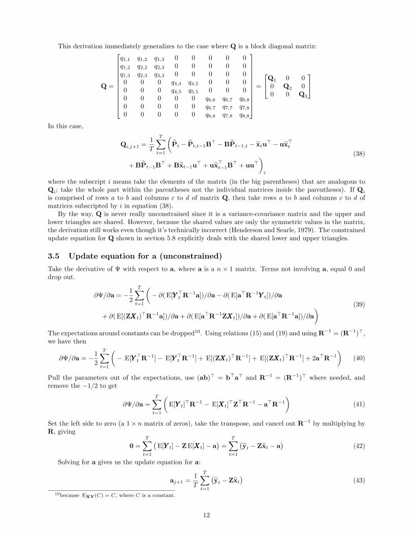
This derivation immediately generalizes to the case where Q is a block diagonal matrix:

Q =

q1,1 q1,2 q1,3 0 0 0 0 0q1,2 q2,2 q2,3 0 0 0 0 0q1,3 q2,3 q3,3 0 0 0 0 00 0 0 q4,4 q4,5 0 0 00 0 0 q4,5 q5,5 0 0 00 0 0 0 0 q6,6 q6,7 q6,8

0 0 0 0 0 q6,7 q7,7 q7,8

0 0 0 0 0 q6,8 q7,8 q8,8

=

Q1 0 00 Q2 00 0 Q3

In this case,

Qi,j+1 =1

T

T∑t=1

(Pt − Pt,t−1B



> + ux>t−1B> + uu>

)i

(38)

where the subscript i means take the elements of the matrix (in the big parentheses) that are analogous toQi; take the whole part within the parentheses not the individual matrices inside the parentheses). If Qi

is comprised of rows a to b and columns c to d of matrix Q, then take rows a to b and columns c to d ofmatrices subscripted by i in equation (38).

By the way, Q is never really unconstrained since it is a variance-covariance matrix and the upper andlower triangles are shared. However, because the shared values are only the symmetric values in the matrix,the derivation still works even though it’s technically incorrect (Henderson and Searle, 1979). The constrainedupdate equation for Q shown in section 5.8 explicitly deals with the shared lower and upper triangles.

3.5 Update equation for a (unconstrained)

Take the derivative of Ψ with respect to a, where a is a n × 1 matrix. Terms not involving a, equal 0 anddrop out.

∂Ψ/∂a = −1

2

T∑t=1

(− ∂( E[YYY >t R−1a])/∂a− ∂( E[a>R−1YYY t])/∂a

+ ∂( E[(ZXXXt)>R−1a])/∂a + ∂( E[a>R−1ZXXXt])/∂a + ∂( E[a>R−1a])/∂a

) (39)

The expectations around constants can be dropped10. Using relations (15) and (19) and using R−1 = (R−1)>,we have then

∂Ψ/∂a = −1

2

T∑t=1

(− E[YYY >t R−1]− E[YYY >t R−1] + E[(ZXXXt)

>R−1] + E[(ZXXXt)>R−1] + 2a>R−1

)(40)

Pull the parameters out of the expectations, use (ab)> = b>a> and R−1 = (R−1)> where needed, andremove the −1/2 to get

∂Ψ/∂a =

T∑t=1

(E[YYY t]

>R−1 − E[XXXt]>Z>R−1 − a>R−1

)(41)

Set the left side to zero (a 1× n matrix of zeros), take the transpose, and cancel out R−1 by multiplying byR, giving

0 =

T∑t=1

(E[YYY t]− Z E[XXXt]− a

)=

T∑t=1

(yt − Zxt − a

)(42)

Solving for a gives us the update equation for a:

aj+1 =1

T

T∑t=1

(yt − Zxt

)(43)

10because EXY(C) = C, where C is a constant.

12

3.6 The update equation for Z (unconstrained)

Take the derivative of Ψ with respect to Z. Terms not involving Z, equal 0 and drop out. The expectationsaround terms involving only constants have been dropped.

∂Ψ/∂Z = (note ∂Z is m× n while Z is n×m)

− 1

2

T∑t=1

(− E[∂(YYY >t R−1ZXXXt)/∂Z]− E[∂((ZXXXt)

>R−1YYY t)/∂Z] + E[∂((ZXXXt)>R−1ZXXXt)/∂Z]

+ E[∂((ZXXXt)>R−1a)/∂Z] + E[∂(a>R−1ZXXXt)/∂Z]

)= −1

2

T∑t=1

(− E[∂(YYY >t R−1ZXXXt)/∂Z]− E[∂(XXX>t Z>R−1YYY t)/∂Z] + E[∂(XXX>t Z>R−1ZXXXt)/∂Z]

+ E[∂(XXX>t Z>R−1a)/∂Z] + E[∂(a>R−1ZXXXt)/∂Z]

)(44)

Using the matrix derivative relations (table 2) and using R−1 = (R−1)>, we get

∂Ψ/∂Z = −1

2

T∑t=1

(− E[XXXtYYY

>t R−1]−E[XXXtYYY

>t R−1]

+ 2 E[XXXtXXX>t Z>R−1] + E[XXXt−1a

>R−1] + E[XXXta>R−1]

) (45)

Pulling the parameters out of the expectations and getting rid of the −1/2, we have

∂Ψ/∂Z =

T∑t=1

(E[XXXtYYY

>t ]R−1 − E[XXXtXXX

>t ]Z>R−1 − E[XXXt]a

>R−1

)(46)

Set the left side to zero (a m× n matrix of zeros), transpose it all, and cancel out R−1 by multiplying by Ron the left, to give

0 =

T∑t=1

(E[YYY tXXX

>t ]− Z E[XXXtXXX

>t ]− a E[XXX>t ]

)=

T∑t=1

(yxt − ZPt − ax>t

)(47)

Solving for Z and noting that Pt is invertible, gives us the new Z:

Zj+1 =

( T∑t=1

(yxt − ax>t

))( T∑t=1

Pt

)−1

(48)

3.7 The update equation for R (unconstrained)

Take the derivative of Ψ with respect to R. Terms not involving R, equal 0 and drop out. The expectationsaround terms involving constants have been removed.

∂Ψ/∂R = −1

2

T∑t=1

(E[∂(YYY >t R−1YYY t)/∂R]− E[∂(YYY >t R−1ZXXXt)/∂R]− E[∂((ZXXXt)

>R−1YYY t)/∂R]

− E[∂(YYY >t R−1a)/∂R]− E[∂(a>R−1YYY t)/∂R] + E[∂((ZXXXt)>R−1ZXXXt)/∂R]

+ E[∂((ZXXXt)>R−1a)/∂R] + E[∂(a>R−1ZXXXt)/∂R] + ∂(a>R−1a)/∂R

)− ∂

(T2

log |R|)/∂R

(49)

We use relations (20) and (17) to do the differentiation. Notice that all the terms in the summation are ofthe form c>R−1b, and thus after differentiation, we group all the c>b inside one set of parentheses. Also

13

there is a minus that comes from equation (20) and cancels out the minus in front of −1/2.

∂Ψ/∂R =1

2

T∑t=1

R−1

(E[YYY tYYY

>t ]− E[YYY t(ZXXXt)

>]− E[ZXXXtYYY>t ]− E[YYY ta

>]− E[aYYY >t ]

+ E[ZXXXt(ZXXXt)>] + E[ZXXXta

>] + E[a(ZXXXt)>] + aa>

)R−1 − T

2R−1

(50)

Pulling the parameters out of the expectations and using (ZYYY t)> = YYY >t Z>, we have

∂Ψ/∂R =1

2

T∑t=1

R−1

(E[YYY tYYY

>t ]− E[YYY tXXX

>t ]Z> − Z E[XXXtYYY

>t ]− E[YYY t]a

> − a E[YYY >t ]

+ Z E[XXXtXXX>t ]Z> + Z E[XXXt]a

> + a E[XXX>t ]Z> + aa>)

R−1 − T

2R−1

(51)

We rewrite the partial derivative in terms of expectations:

∂Ψ/∂R =1

2

T∑t=1

R−1

(Ot − yxtZ

> − Zyx>t − yta

> − ay>t

+ ZPtZ> + Zxta

> + ax>t Z> + aa>)

R−1 − T

2R−1

(52)

Setting this to zero (a n×n matrix of zeros), we cancel out R−1 by multiplying by R twice, once on the leftand once on the right, and get rid of the 1/2.

TR =

T∑t=1

(Ot − yxtZ

> − Zyx>t − yta

> − ay>t + ZPtZ> + Zxta

> + ax>t Z> + aa>)

(53)

We can then solve for R, giving us the new R that maximizes Ψ,

Rj+1 =1

T

T∑t=1

(Ot − yxtZ

> − Zyx>t − yta


> + ax>t Z> + aa>)

(54)

As with Q, this derivation immediately generalizes to a block diagonal matrix:

R =

R1 0 00 R2 00 0 R3

In this case,

Ri,j+1 =1

T

T∑t=1

(Ot − yxtZ

> − Zyx>t − yta


> + ax>t Z> + aa>)i

(55)

where the subscript i means we take the elements in the matrix in the big parentheses that are analogous toRi. If Ri is comprised of rows a to b and columns c to d of matrix R, then we take rows a to b and columnsc to d of matrix subscripted by i in equation (55).

3.8 Update equation for ξ and Λ (unconstrained), stochastic initial state

Shumway and Stoffer (2006) and Ghahramani and Hinton (1996) imply in their discussion of the EM algorithmthat both ξ and Λ can be estimated (though not simultaneously). Harvey (1989), however, discusses thatthere are only two allowable cases: xxx0 is treated as fixed (Λ = 0) and equal to the unknown parameter ξ orxxx0 is treated as stochastic with a known mean ξ and variance Λ. For completeness, we show here the updateequation in the case of xxx0 stochastic with unknown mean ξ and variance Λ (a case that Harvey (1989) saysis not consistent).

14

We proceed as before and solve for the new ξ by minimizing Ψ. Take the derivative of Ψ with respect toξ . Terms not involving ξ, equal 0 and drop out.

∂Ψ/∂ξ = −1

2

(− ∂( E[ξ>Λ−1XXX0])/∂ξ − ∂( E[XXX>0 Λ−1ξ])/∂ξ + ∂(ξ>Λ−1ξ)/∂ξ

)(56)

Using relations (15) and (19) and using Λ−1 = (Λ−1)>, we have

∂Ψ/∂ξ = −1

2

(− E[XXX>0 Λ−1]− E[XXX>0 Λ−1] + 2ξ>Λ−1

)(57)

Pulling the parameters out of the expectations, we get

∂Ψ/∂ξ = −1

2

(− 2 E[XXX>0 ]Λ−1 + 2ξ>Λ−1

)(58)

We then set the left side to zero, take the transpose, and cancel out −1/2 and Λ−1 (by noting that it is avariance-covariance matrix and is invertible).

0 =(Λ−1 E[XXX0] + Λ−1ξ

)= (x0 − ξ) (59)

Thus,ξj+1 = x0 (60)

x0 is the expected value of XXX0 conditioned on the data from t = 1 to T , which comes from the Kalmansmoother recursions with initial conditions defined as E[XXX0|YYY 0 = yyy0] ≡ ξ and var(XXX0XXX

>0 |YYY 0 = yyy0) ≡ Λ. A

similar set of steps gets us to the update equation for Λ,

Λj+1 = V0 (61)

V0 is the variance ofXXX0 conditioned on the data from t = 1 to T and is an output from the Kalman smootherrecursions.

If the initial state is defined as at t = 1 instead of t = 0, the update equation is derived in an identicalfashion and the update equation is similar:

ξj+1 = x1 (62)

Λj+1 = V1 (63)

These are output from the Kalman smoother recursions with initial conditions defined as E[XXX1|YYY 0 = yyy0] ≡ ξand var(XXX1XXX

>1 |YYY 0 = yyy0) ≡ Λ. Notice that the recursions are initialized slightly differently; you will see the

Kalman filter and smoother equations presented with both types of initializations depending on whether theauthor defines the initial state at t = 0 or t = 1.

3.9 Update equation for ξ (unconstrained), fixed xxx0

For the case where xxx0 is treated as fixed, i.e. as another parameter, then there is no Λ, and we need tomaximize ∂Ψ/∂ξ using the slightly different Ψ shown in equation (7). Now ξ appears in the state equationpart of the likelihood.

∂Ψ/∂ξ = −1

2

(− E[∂(XXX>1 Q−1Bξ)/∂ξ]− E[∂((Bξ)>Q−1XXX1)/∂ξ] + E[∂((Bξ)>Q−1(Bξ))/∂ξ]

+ E[∂((Bξ)>Q−1u)/∂ξ] + E[∂(u>Q−1Bξ)/∂ξ]

)= −1

2

(− E[∂(XXX>1 Q−1Bξ)/∂ξ]− E[∂(ξ>B>Q−1XXX1)/∂ξ] + E[∂(ξ>B>Q−1(Bξ))/∂ξ]

+ E[∂(ξ>B>Q−1u)/∂ξ] + E[∂(u>Q−1Bξ)/∂ξ]

)(64)

After pulling the constants out of the expectations, we use relations (16) and (18) to take the derivative:

∂Ψ/∂ξ = −1

2

(− E[XXX1]>Q−1B− E[XXX1]>Q−1B + 2ξ>B>Q−1B + u>Q−1B + u>Q−1B

)(65)

15


∂Ψ/∂ξ = E[XXX1]>Q−1B− ξ>B>Q−1B− u>Q−1B (66)

To solve for ξ, set the left side to zero (an m × 1 matrix of zeros), transpose the whole equation, and thencancel out B>Q−1B by multiplying by its inverse on the left, and solve for ξ. This step requires that thisinverse exists.

ξ = (B>Q−1B)−1B>Q−1( E[XXX1]− u) (67)

Thus, in terms of the Kalman filter/smoother output the new ξ for EM iteration j + 1 is

ξj+1 = (B>Q−1B)−1B>Q−1(x1 − u) (68)

Note that using, x0 output from the Kalman smoother would not work since Λ = 0. As a result, ξj+1 ≡ ξjin the EM algorithm, and it is impossible to move away from your starting condition for ξ.

This is conceptually similar to using a generalized least squares estimate of ξ to concentrate it out of thelikelihood as discussed in Harvey (1989), section 3.4.4. However, in the context of the EM algorithm, dealingwith the fixed xxx0 case requires nothing special; one simply takes care to use the likelihood for the case wherexxx0 is treated as an unknown parameter (equation 7). For the other parameters, the update equations arethe same whether one uses the log-likelihood equation with xxx0 treated as stochastic (equation 6) or fixed(equation 7).

If your MARSS model is stationary11 and your data appear stationary, however, equation (67) probablyis not what you want to use. The estimate of ξ will be the maximum-likelihood value, but it will not bedrawn from the stationary distribution; instead it could be some wildly different value that happens to givethe maximum-likelihood. If you are modeling the data as stationary, then you should probably assume thatξ is drawn from the stationary distribution of the XXX’s, which is some function of your model parameters.This would mean that the model parameters would enter the part of the likelihood that involves ξ and Λ.Since you probably don’t want to do that (if might start to get circular), you might try an iterative processto get decent ξ and Λ or try fixing ξ and estimating Λ (above). You can fix ξ at, say, zero, by making surethe model you fit has a stationary distribution with mean zero. You might also need to demean your data(or estimate the a term to account for non-zero mean data). A second approach is to estimate xxx1 as theinitial state instead of xxx0.

3.10 Update equation for ξ (unconstrained), fixed xxx1

In some cases, the estimate of xxx0 from xxx1 using equation 68 will be highly sensitive to small changes in theparameters. This is particularly the case for certain B matrices, even if they are stationary. The result isthat your ξ estimate is wildly different from the data at t = 1. The estimates are correct given how youdefined the model, just not realistic given the data. In this case, you can specify ξ as being the value of xxx att = 1 instead of t = 0. That way, the data at t = 1 will constrain the estimated ξ. In this case, we treat xxx1

as fixed but unknown parameter ξ. The likelihood is then:


1


T∑1

1

2log |R|

−T∑2

1


T∑1

1

2log |Q|

(69)

∂Ψ/∂ξ = −1

2

(− E[∂(YYY >1 R−1Zξ)/∂ξ]− E[∂((Zξ)>R−1YYY 1)/∂ξ] + E[∂((Zξ)>R−1(Zξ))/∂ξ]

+ E[∂((Zξ)>R−1a)/∂ξ] + E[∂(a>R−1Zξ)/∂ξ]

)− 1

2

(− E[∂(XXX>2 Q−1Bξ)/∂ξ]− E[∂((Bξ)>Q−1XXX2)/∂ξ] + E[∂((Bξ)>Q−1(Bξ))/∂ξ]

+ E[∂((Bξ)>Q−1u)/∂ξ] + E[∂(u>Q−1Bξ)/∂ξ]

)(70)

11meaning the XXX’s have a stationary distribution

16

Note that the second summation starts at t = 2 and ξ is xxx1 instead of xxx0.After pulling the constants out of the expectations, we use relations (16) and (18) to take the derivative:

∂Ψ/∂ξ = −1

2

(− E[YYY 1]>R−1Z− E[YYY 1]>R−1Z + 2ξ>Z>R−1Z + a>R−1Z + a>R−1Z

)− 1

2

(− E[XXX2]>Q−1B− E[XXX2]>Q−1B + 2ξ>B>Q−1B + u>Q−1B + u>Q−1B

) (71)


∂Ψ/∂ξ = E[YYY 1]>R−1Z− ξ>Z>R−1Z− a>R−1Z + E[XXX2]>Q−1B− ξ>B>Q−1B− u>Q−1B

= −ξ>(Z>R−1Z + B>Q−1B) + E[YYY 1]>R−1Z− a>R−1Z + E[XXX2]>Q−1B− u>Q−1B(72)

To solve for ξ, set the left side to zero (an m × 1 matrix of zeros), transpose the whole equation, and solvefor ξ.

ξ = (Z>R−1Z + B>Q−1B)−1(Z>R−1( E[YYY 1]− a) + B>Q−1( E[XXX2]− u)) (73)

Thus, when ξ ≡ xxx1, the new ξ for EM iteration j + 1 is

ξj+1 = (Z>R−1Z + B>Q−1B)−1(Z>R−1(y1 − a) + B>Q−1(x2 − u)) (74)

4 The time-varying MARSS model with linear constraints

The first part of this report dealt with the case of a MARSS model (equation 1) where the parameters aretime-constant and where all the elements in a parameter matrix are estimated with no constraints. I willnow describe the derivation of an EM algorithm to solve a much more general MARSS model (equation75), which is a time-varying MARSS model where the MARSS parameter matrices are written as a linearequation f + Dm. This is a very general form of a MARSS model, of which many (most) multivariateautoregressive Gaussian models are a special case. This general MARSS model includes as special cases,MARSS models with covariates (many VARSS models with exogeneous variables), multivariate AR lag-pmodels and multivariate moving average models, and MARSS models with linear constraints placed on theelements within the model parameters. The objective is to derive one EM algorithm for the whole class, thusa uniform approach to fitting these models.

The time-varying MARSS model is written:

xxxt = Btxxxt−1 + ut + Gtwt, where Wt ∼ MVN(0,Qt) (75a)

yyyt = Ztxxxt + at + Htvt, where Vt ∼ MVN(0,Rt) (75b)

xxxt0 = ξ + Fl, where t0 = 0 or t0 = 1 (75c)

L ∼ MVN(0,Λ) (75d)[wt

vt

]∼ MVN(0,Σ), Σ =

[Qt 00 Rt

](75e)

This looks quite similar to the previous non-time varying MARSS model, but now the model parameters, B,u, Q, Z, a and R, have a t subscript and we have a multiplier matrix on the error terms vt, wt, l. The Gt

multiplier is m× s, so we now have s state errors instead of m. The Ht multiplier is n× k, so we now have kobservation errors instead of n. The F multiplier is m× j, so now we can have some initial states (j of them)be stochastic and others be fixed. I assume that appropriate constraints are put on G and H so that theresulting MARSS model is not under- or over-constrained12. The notation/presentation here was influencedby SJ Koopman’s work, esp. Koopman and Ooms (2011) and Koopman (1993), but in these works, Qt andRt equal I and the variance-covariance structures are instead specified only by Ht and Gt. I keep Qt andRt in my formulation as it seems more intuitive (to me) in the context of the EM algorithm and the requiredjoint-likelihood function.

12For example, if both G and H are column vectors, then the system is over-constrained and has no solution.

17

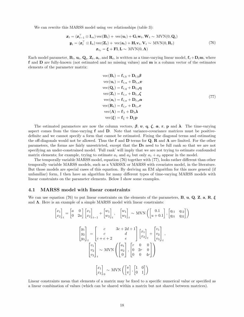
We can rewrite this MARSS model using vec relationships (table 3):

xxxt = (xxx>t−1 ⊗ Im) vec(Bt) + vec(ut) + Gtwt,Wt ∼ MVN(0,Qt)

yyyt = (xxx>t ⊗ In) vec(Zt) + vec(at) + Htvt,Vt ∼ MVN(0,Rt)

xxxt0 = ξ + Fl,L ∼ MVN(0,Λ)

(76)

Each model parameter, Bt, ut, Qt, Zt, at, and Rt, is written as a time-varying linear model, f t+Dtm, wheref and D are fully-known (not estimated and no missing values) and m is a column vector of the estimateselements of the parameter matrix:

vec(Bt) = f t,b + Dt,bβββ

vec(ut) = f t,u + Dt,uυυυ

vec(Qt) = f t,q + Dt,qq

vec(Zt) = f t,z + Dt,zζζζ

vec(at) = f t,a + Dt,aααα

vec(Rt) = f t,r + Dt,rr

vec(Λ) = fλ + Dλλλλ

vec(ξ) = fξ + Dξp

(77)

The estimated parameters are now the column vectors, βββ, υυυ, q, ζζζ, ααα, r, p and λλλ. The time-varyingaspect comes from the time-varying f and D. Note that variance-covariance matrices must be positive-definite and we cannot specify a form that cannot be estimated. Fixing the diagonal terms and estimatingthe off-diagonals would not be allowed. Thus the f and D terms for Q, R and Λ are limited. For the otherparameters, the forms are fairly unrestricted, except that the Ds need to be full rank so that we are notspecifying an under-constrained model. ’Full rank’ will imply that we are not trying to estimate confoundedmatrix elements; for example, trying to estimate a1 and a2 but only a1 + a2 appear in the model.

The temporally variable MARSS model, equation (76) together with (77), looks rather different than othertemporally variable MARSS models, such as a VARSSX or MARSS with covariates model, in the literature.But those models are special cases of this equation. By deriving an EM algorithm for this more general (ifunfamiliar) form, I then have an algorithm for many different types of time-varying MARSS models withlinear constraints on the parameter elements. Below I show some examples.

4.1 MARSS model with linear constraints

We can use equation (76) to put linear constraints on the elements of the parameters, B, u, Q, Z, a, R, ξand Λ. Here is an example of a simple MARSS model with linear constraints:[

x1

x2

]t

=

[a 00 2a

] [x1

x2

]t−1

+

[w1

w2

]t

,

[w1

w2

]t

∼ MVN

([0.1

u+ 0.1

],

[q11 q12

q21 q22

])y1

y2

y3

t

=

c 3c+ 2d+ 1c d

c+ e+ 2 e

[x1

x2

]t

+

v1

v2

v3

t

,

v1

v2

v3

t

∼ MVN

a1

a2

0

,r 0 0

0 2r 00 0 4r

[x1

x2

]0

∼ MVN

([ππ

],

[1 00 1

])Linear constraints mean that elements of a matrix may be fixed to a specific numerical value or specified asa linear combination of values (which can be shared within a matrix but not shared between matrices).

18

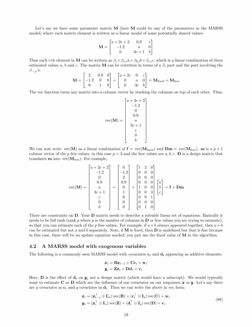
Let’s say we have some parameter matrix M (here M could be any of the parameters in the MARSSmodel) where each matrix element is written as a linear model of some potentially shared values:

M =

a+ 2c+ 2 0.9 c−1.2 a 0

0 3c+ 1 b

Thus each i-th element in M can be written as βi+βa,ia+βb,ib+βc,ic, which is a linear combination of threeestimated values a, b and c. The matrix M can be rewritten in terms of a βi part and the part involving theβ−,j ’s:

M =

2 0.9 0−1.2 0 0

0 1 0

+

a+ 2c 0 c0 a 00 3c b

= Mfixed + Mfree

The vec function turns any matrix into a column vector by stacking the columns on top of each other. Thus,

vec(M) =

a+ 2c+ 2−1.2

00.9a

3c+ 1c0b

We can now write vec(M) as a linear combination of f = vec(Mfixed) and Dm = vec(Mfree). m is a p× 1column vector of the p free values, in this case p = 3 and the free values are a, b, c. D is a design matrix thattranslates m into vec(Mfree). For example,

vec(M) =

a+ 2c+ 2−1.2

00.9a

3c+ 1c0b

=

0−1.2

20.901000

+

1 2 00 0 00 0 00 0 01 0 00 0 30 0 10 0 00 1 0

abc

= f + Dm

There are constraints on D. Your D matrix needs to describe a solvable linear set of equations. Basically itneeds to be full rank (rank p where p is the number of columns in D or free values you are trying to estimate),so that you can estimate each of the p free values. For example, if a+ b always appeared together, then a+ bcan be estimated but not a and b separately. Note, if M is fixed, then D is undefined but that is fine becausein this case, there will be no update equation needed; you just use the fixed value of M in the algorithm.

4.2 A MARSS model with exogenous variables

The following is a commonly seen MARSS model with covariates ct and dt appearing as additive elements:

xxxt = Bxxxt−1 + Cct + wt

yyyt = Zxxxt + Ddt + vt

Here, D is the effect of dt on yyyt not a design matrix (which would have a subscript). We would typicallywant to estimate C or D which are the influence of our covariates on our responses, xxx or yyy. Let’s say thereare p covariates in ct and q covariates in dt. Then we can write the above in vec form:

xxxt = (xxx>t−1 ⊗ Im) vec(B) + (c>t ⊗ Ip) vec(C) + wt

yyyt = (xxx>t ⊗ In) vec(Z) + (d>t ⊗ Iq) vec(D) + vt(88)

19

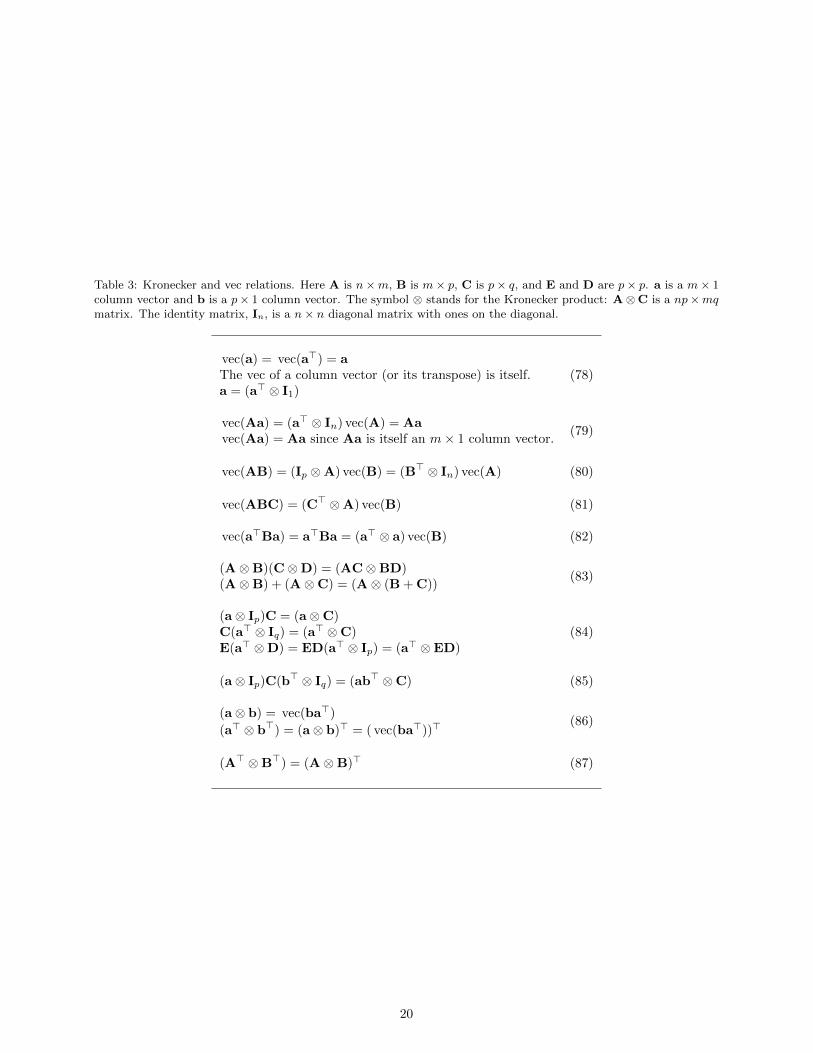
Table 3: Kronecker and vec relations. Here A is n×m, B is m× p, C is p× q, and E and D are p× p. a is a m× 1column vector and b is a p× 1 column vector. The symbol ⊗ stands for the Kronecker product: A⊗C is a np×mqmatrix. The identity matrix, In, is a n× n diagonal matrix with ones on the diagonal.

vec(a) = vec(a>) = a(78)The vec of a column vector (or its transpose) is itself.

a = (a> ⊗ I1)

vec(Aa) = (a> ⊗ In) vec(A) = Aa(79)

vec(Aa) = Aa since Aa is itself an m× 1 column vector.

vec(AB) = (Ip ⊗A) vec(B) = (B> ⊗ In) vec(A) (80)

vec(ABC) = (C> ⊗A) vec(B) (81)

vec(a>Ba) = a>Ba = (a> ⊗ a) vec(B) (82)

(A⊗B)(C⊗D) = (AC⊗BD)(83)

(A⊗B) + (A⊗C) = (A⊗ (B + C))

(a⊗ Ip)C = (a⊗C)(84)C(a> ⊗ Iq) = (a> ⊗C)

E(a> ⊗D) = ED(a> ⊗ Ip) = (a> ⊗ED)

(a⊗ Ip)C(b> ⊗ Iq) = (ab> ⊗C) (85)

(a⊗ b) = vec(ba>)(86)

(a> ⊗ b>) = (a⊗ b)> = ( vec(ba>))>

(A> ⊗B>) = (A⊗B)> (87)

20

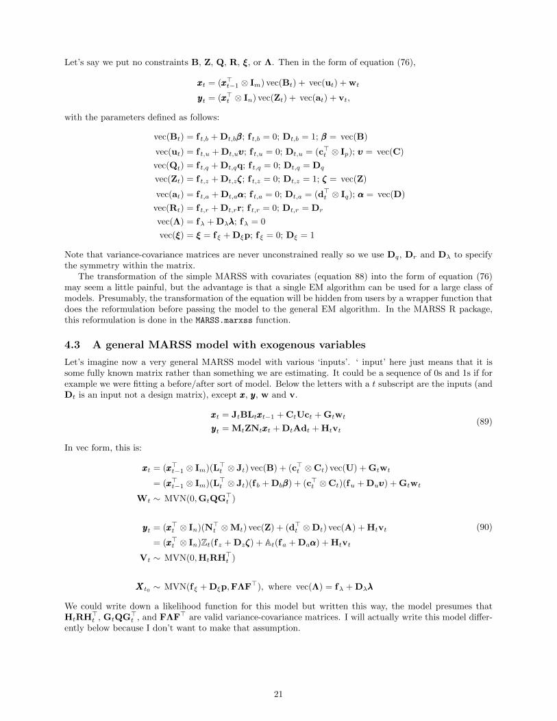
Let’s say we put no constraints B, Z, Q, R, ξ, or Λ. Then in the form of equation (76),

xxxt = (xxx>t−1 ⊗ Im) vec(Bt) + vec(ut) + wt

yyyt = (xxx>t ⊗ In) vec(Zt) + vec(at) + vt,

with the parameters defined as follows:

vec(Bt) = f t,b + Dt,bβββ; f t,b = 0; Dt,b = 1; βββ = vec(B)

vec(ut) = f t,u + Dt,uυυυ; f t,u = 0; Dt,u = (c>t ⊗ Ip); υυυ = vec(C)

vec(Qt) = f t,q + Dt,qq; f t,q = 0; Dt,q = Dq

vec(Zt) = f t,z + Dt,zζζζ; f t,z = 0; Dt,z = 1; ζζζ = vec(Z)

vec(at) = f t,a + Dt,aααα; f t,a = 0; Dt,a = (d>t ⊗ Iq); ααα = vec(D)

vec(Rt) = f t,r + Dt,rr; f t,r = 0; Dt,r = Dr

vec(Λ) = fλ + Dλλλλ; fλ = 0

vec(ξ) = ξ = fξ + Dξp; fξ = 0; Dξ = 1

Note that variance-covariance matrices are never unconstrained really so we use Dq, Dr and Dλ to specifythe symmetry within the matrix.

The transformation of the simple MARSS with covariates (equation 88) into the form of equation (76)may seem a little painful, but the advantage is that a single EM algorithm can be used for a large class ofmodels. Presumably, the transformation of the equation will be hidden from users by a wrapper function thatdoes the reformulation before passing the model to the general EM algorithm. In the MARSS R package,this reformulation is done in the MARSS.marxss function.

4.3 A general MARSS model with exogenous variables

Let’s imagine now a very general MARSS model with various ‘inputs’. ‘ input’ here just means that it issome fully known matrix rather than something we are estimating. It could be a sequence of 0s and 1s if forexample we were fitting a before/after sort of model. Below the letters with a t subscript are the inputs (andDt is an input not a design matrix), except xxx, yyy, w and v.

xxxt = JtBLtxxxt−1 + CtUct + Gtwt

yyyt = MtZNtxxxt + DtAdt + Htvt(89)

In vec form, this is:

xxxt = (xxx>t−1 ⊗ Im)(L>t ⊗ Jt) vec(B) + (c>t ⊗Ct) vec(U) + Gtwt

= (xxx>t−1 ⊗ Im)(L>t ⊗ Jt)(f b + Dbβββ) + (c>t ⊗Ct)(fu + Duυυυ) + Gtwt

Wt ∼ MVN(0,GtQG>t )

yyyt = (xxx>t ⊗ In)(N>t ⊗Mt) vec(Z) + (d>t ⊗Dt) vec(A) + Htvt

= (xxx>t ⊗ In)Zt(fz + Dzζζζ) + At(fa + Daααα) + Htvt

Vt ∼ MVN(0,HtRH>t )

XXXt0 ∼ MVN(fξ + Dξp,FΛF>), where vec(Λ) = fλ + Dλλλλ

(90)

We could write down a likelihood function for this model but written this way, the model presumes thatHtRH>t , GtQG>t , and FΛF> are valid variance-covariance matrices. I will actually write this model differ-ently below because I don’t want to make that assumption.

21

We define the f and D parameters as follows.

vec(Bt) = f t,b + Dt,bβββ = (L>t ⊗ Jt)f b + (L>t ⊗ Jt)Dbβββ

vec(ut) = f t,u + Dt,uυυυ = (c>t ⊗Ct)fu + (c>t ⊗Ct)Duυυυ

vec(Qt) = f t,q + Dt,qq = (Gt ⊗Gt)fq + (Gt ⊗Gt)Dqq

vec(Zt) = f t,z + Dt,zζζζ = (N>t ⊗Mt)fz + (N>t ⊗Mt)Dzζζζ

vec(at) = f t,a + Dt,aααα = (d>t ⊗Dt)fa + (d>t ⊗Dt)Daααα

vec(Rt) = f t,r + Dt,rr = (Ht ⊗Ht)fq + (Ht ⊗Ht)Drr

vec(Λ) = fλ + Dλλλλ = 0 + Dλλλλ

vec(ξ) = ξ = fξ + Dξp = 0 + 1p

Here, for example f b and Db indicate the linear constraints on B and f t,b is (L>t ⊗Jt)f b and Dt,b is (L>t ⊗Jt)Db.The elements of B that are being estimated are βββ arranged as a column vector.

As usual, this reformulation looks cumbersome, but would be hidden from the user presumably.

4.4 The expected log-likelihood function

As mentioned above, we do not necessarily want to assume that HtRtH>t , GtQtG

>t , and FΛF> are valid

variance-covariance matrices. This would rule out many MARSS models that we would like to fit. For

example, if Q = σ2 and G =

111

, GQG> would be an invalid variance-variance matrix. However, this is

a valid MARSS model. We do need to be careful that Ht and Gt are specified such that the model has a

solution. For example, a model where both G and H are

111

would not be solvable for all yyy.

Instead I will define Φt = (G>t Gt)−1G>t , Ξt = (H>t Ht)

−1H>t , and Π = (F>F)−1F>. I then require thatthe inverses of G>t Gt, H>t Ht, and F>F exist and that f t,q + Dt,qq, f t,r + Dt,rr, and fλ + Dλλλλ specify validvariance-covariance matrices. These are much less stringent restrictions.

For the purpose of writing down the expected log-likelihood, our MARSS model is now written

Φtxxxt = Φt(xxx>t−1 ⊗ Im) vec(Bt) + Φt vec(ut) + wt, where Wt ∼ MVN(0,Qt)

Ξtyyyt = Ξt(xxx>t ⊗ In) vec(Zt) + Ξt vec(at) + vt, where Vt ∼ MVN(0,Rt)

Πxxxt0 = Πξ + l, where L ∼ MVN(0,Λ)

(91)

As mentioned before, this relies on G and H having forms that do not lead to over- or under-constrainedlinear systems.

To derive the EM update equations, we need the expected log-likelihood function for the time-varyingMARSS model. Using equation (91), we get

EXY[log L(YYY ,XXX; Θ)] = −1

2EXY

( T∑1

(YYY t − (XXX>t ⊗ Im) vec(Zt)− vec(at))>Ξ>t R−1

t Ξt

(YYY t − (XXX>t ⊗ Im) vec(Zt)− vec(at)) +

T∑1

log |Rt|

+

T∑t0+1

(XXXt − (XXX>t−1 ⊗ Im) vec(Bt)− vec(ut))>Φ>t Q−1

t Φt

(XXXt − (XXX>t−1 ⊗ Im) vec(Bt)− vec(ut)) +

T∑t0+1

log |Qt|

+ (XXXt0 − vec(ξ))>Π>Λ−1Π(XXXt0 − vec(ξ)) + log |Λ|+ log 2π

)

(92)

22

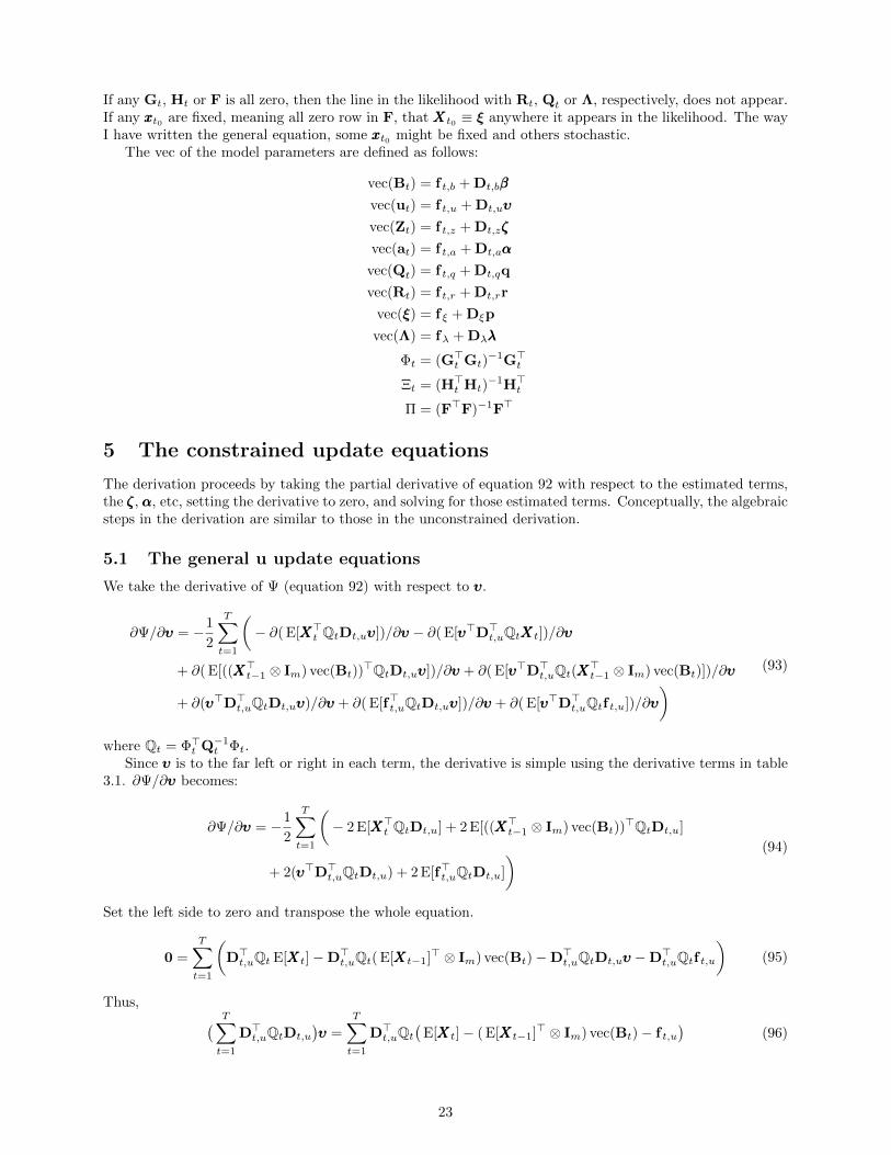
If any Gt, Ht or F is all zero, then the line in the likelihood with Rt, Qt or Λ, respectively, does not appear.If any xxxt0 are fixed, meaning all zero row in F, that XXXt0 ≡ ξ anywhere it appears in the likelihood. The wayI have written the general equation, some xxxt0 might be fixed and others stochastic.

The vec of the model parameters are defined as follows:

vec(Bt) = f t,b + Dt,bβββ

vec(ut) = f t,u + Dt,uυυυ

vec(Zt) = f t,z + Dt,zζζζ

vec(at) = f t,a + Dt,aααα

vec(Qt) = f t,q + Dt,qq

vec(Rt) = f t,r + Dt,rr

vec(ξ) = fξ + Dξp

vec(Λ) = fλ + Dλλλλ

Φt = (G>t Gt)−1G>t

Ξt = (H>t Ht)−1H>t

Π = (F>F)−1F>

5 The constrained update equations

The derivation proceeds by taking the partial derivative of equation 92 with respect to the estimated terms,the ζζζ, ααα, etc, setting the derivative to zero, and solving for those estimated terms. Conceptually, the algebraicsteps in the derivation are similar to those in the unconstrained derivation.

5.1 The general u update equations

We take the derivative of Ψ (equation 92) with respect to υυυ.

∂Ψ/∂υυυ = −1

2

T∑t=1

(− ∂( E[XXX>t QtDt,uυυυ])/∂υυυ − ∂( E[υυυ>D>t,uQtXXXt])/∂υυυ

+ ∂( E[((XXX>t−1 ⊗ Im) vec(Bt))>QtDt,uυυυ])/∂υυυ + ∂( E[υυυ>D>t,uQt(XXX

>t−1 ⊗ Im) vec(Bt)])/∂υυυ

+ ∂(υυυ>D>t,uQtDt,uυυυ)/∂υυυ + ∂( E[f>t,uQtDt,uυυυ])/∂υυυ + ∂( E[υυυ>D>t,uQtf t,u])/∂υυυ

) (93)

where Qt = Φ>t Q−1t Φt.

Since υυυ is to the far left or right in each term, the derivative is simple using the derivative terms in table3.1. ∂Ψ/∂υυυ becomes:

∂Ψ/∂υυυ = −1

2

T∑t=1

(− 2 E[XXX>t QtDt,u] + 2 E[((XXX>t−1 ⊗ Im) vec(Bt))

>QtDt,u]

+ 2(υυυ>D>t,uQtDt,u) + 2 E[f>t,uQtDt,u]

) (94)

Set the left side to zero and transpose the whole equation.

0 =

T∑t=1

(D>t,uQt E[XXXt]−D>t,uQt( E[XXXt−1]> ⊗ Im) vec(Bt)−D>t,uQtDt,uυυυ −D>t,uQtf t,u

)(95)

Thus, ( T∑t=1

D>t,uQtDt,u

)υυυ =

T∑t=1

D>t,uQt(

E[XXXt]− ( E[XXXt−1]> ⊗ Im) vec(Bt)− f t,u)

(96)

23

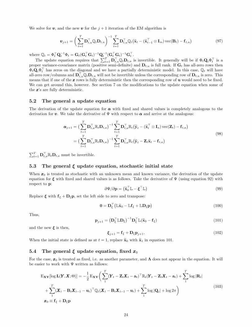
We solve for υυυ, and the new υυυ for the j + 1 iteration of the EM algorithm is

υυυj+1 =

( T∑t=1

D>t,uQtDt,u

)−1 T∑t=1

D>t,uQt(xt − (x>t−1 ⊗ Im) vec(Bt)− f t,u

)(97)

where Qt = Φ>t Q−1t Φt = Gt(G

>t Gt)

−1Q−1t (G>t Gt)

−1G>t .

The update equation requires that∑Tt=1 D>t,uQtDt,u is invertible. It generally will be if ΦtQtΦ

>t is a

proper variance-covariance matrix (positive semi-definite) and Dt,u is full rank. If Gt has all-zero rows thenΦtQtΦ

>t has zeros on the diagonal and we have a partially deterministic model. In this case, Qt will have

all-zero row/columns and D>t,uQtDt,u will not be invertible unless the corresponding row of Dt,u is zero. Thismeans that if one of the xxx rows is fully deterministic then the corresponding row of u would need to be fixed.We can get around this, however. See section 7 on the modifications to the update equation when some ofthe xxx’s are fully deterministic.

5.2 The general a update equation

The derivation of the update equation for ααα with fixed and shared values is completely analogous to thederivation for υυυ. We take the derivative of Ψ with respect to ααα and arrive at the analogous:

αααj+1 =( T∑t=1

D>t,aRtDt,a

)−1T∑t=1

D>t,aRt(yt − (x>t ⊗ In) vec(Zt)− f t,a

)=( T∑t=1

D>t,aRtDt,a

)−1T∑t=1

D>t,aRt(yt − Ztxt − f t,a

) (98)

∑Tt=1 D>t,aRtDt,a must be invertible.

5.3 The general ξ update equation, stochastic initial state

When xxx0 is treated as stochastic with an unknown mean and known variance, the derivation of the updateequation for ξ with fixed and shared values is as follows. Take the derivative of Ψ (using equation 92) withrespect to p:

∂Ψ/∂p =(x>0 L− ξ>L

)(99)

Replace ξ with fξ + Dξp, set the left side to zero and transpose:

0 = D>ξ(Lx0 − Lfξ + LDξp

)(100)

Thus,

pj+1 =(D>ξ LDξ

)−1D>ξ L(x0 − fξ) (101)

and the new ξ is then,ξj+1 = fξ + Dξpj+1, (102)

When the initial state is defined as at t = 1, replace x0 with x1 in equation 101.

5.4 The general ξ update equation, fixed xxx0

For the case, xxx0 is treated as fixed, i.e. as another parameter, and Λ does not appear in the equation. It willbe easier to work with Ψ written as follows:


2EXY

( T∑1

(YYY t − ZtXXXt − at)>Rt(YYY t − ZtXXXt − at) +

T∑1

log |Rt|

+

T∑1

(XXXt −BtXXXt−1 − ut)>Qt(XXXt −BtXXXt−1 − ut) +

T∑1

log |Qt|+ log 2π

)xxx0 ≡ fξ + Dξp

(103)

24

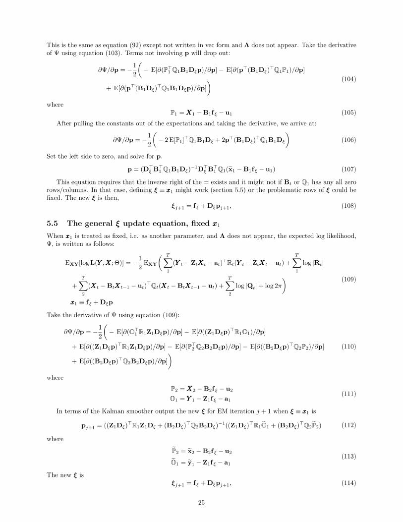
This is the same as equation (92) except not written in vec form and Λ does not appear. Take the derivativeof Ψ using equation (103). Terms not involving p will drop out:

∂Ψ/∂p = −1

2

(− E[∂(P>1 Q1B1Dξp)/∂p]− E[∂(p>(B1Dξ)

>Q1P1)/∂p]

+ E[∂(p>(B1Dξ)>Q1B1Dξp)/∂p]

) (104)

whereP1 = XXX1 −B1fξ − u1 (105)

After pulling the constants out of the expectations and taking the derivative, we arrive at:

∂Ψ/∂p = −1

2

(− 2 E[P1]>Q1B1Dξ + 2p>(B1Dξ)

>Q1B1Dξ

)(106)

Set the left side to zero, and solve for p.

p = (D>ξ B>1 Q1B1Dξ)−1D>ξ B>1 Q1(x1 −B1fξ − u1) (107)

This equation requires that the inverse right of the = exists and it might not if Bt or Q1 has any all zerorows/columns. In that case, defining ξ ≡ xxx1 might work (section 5.5) or the problematic rows of ξ could befixed. The new ξ is then,

ξj+1 = fξ + Dξpj+1, (108)

5.5 The general ξ update equation, fixed xxx1

When xxx1 is treated as fixed, i.e. as another parameter, and Λ does not appear, the expected log likelihood,Ψ, is written as follows:


2EXY

( T∑1

(YYY t − ZtXXXt − at)>Rt(YYY t − ZtXXXt − at) +

T∑1

log |Rt|

+

T∑2

(XXXt −BtXXXt−1 − ut)>Qt(XXXt −BtXXXt−1 − ut) +

T∑2

log |Qt|+ log 2π

)xxx1 ≡ fξ + Dξp

(109)

Take the derivative of Ψ using equation (109):

∂Ψ/∂p = −1

2

(− E[∂(O>1 R1Z1Dξp)/∂p]− E[∂((Z1Dξp)>R1O1)/∂p]

+ E[∂((Z1Dξp)>R1Z1Dξp)/∂p]− E[∂(P>2 Q2B2Dξp)/∂p]− E[∂((B2Dξp)>Q2P2)/∂p]

+ E[∂((B2Dξp)>Q2B2Dξp)/∂p]

) (110)

where

P2 = XXX2 −B2fξ − u2

O1 = YYY 1 − Z1fξ − a1

(111)

In terms of the Kalman smoother output the new ξ for EM iteration j + 1 when ξ ≡ xxx1 is

pj+1 = ((Z1Dξ)>R1Z1Dξ + (B2Dξ)

>Q2B2Dξ)−1((Z1Dξ)

>R1O1 + (B2Dξ)>Q2P2) (112)

where

P2 = x2 −B2fξ − u2

O1 = y1 − Z1fξ − a1

(113)

The new ξ isξj+1 = fξ + Dξpj+1, (114)

25

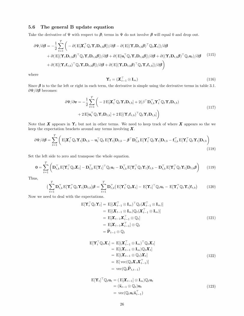
5.6 The general B update equation

Take the derivative of Ψ with respect to βββ; terms in Ψ do not involve βββ will equal 0 and drop out.

∂Ψ/∂βββ = −1

2

T∑t=1

(− ∂( E[XXX>t QtΥtDt,bβββ])/∂βββ − ∂( E[(ΥtDt,bβββ)>QtXXXt])/∂βββ

+ ∂( E[(ΥtDt,bβββ)>QtΥtDt,bβββ])/∂βββ + ∂( E[u>t QtΥtDt,bβββ])/∂βββ + ∂((ΥtDt,bβββ)>Qtut)/∂βββ

+ ∂( E[(Υtf t,b)>QtΥtDt,bβββ])/∂βββ + ∂( E[(ΥtDt,bβββ)>QtΥtf t,b])/∂βββ

) (115)

whereΥt = (XXX>t−1 ⊗ Im) (116)

Since βββ is to the far left or right in each term, the derivative is simple using the derivative terms in table 3.1.∂Ψ/∂βββ becomes:

∂Ψ/∂υυυ = −1

2

T∑t=1

(− 2 E[XXX>t QtΥtDt,b] + 2(β>D>t,bΥ

>t QtΥtDt,b)

+ 2 E[u>t QtΥtDt,b] + 2 E[(Υtf t,b)>QtΥtDt,b]

) (117)

Note that XXX appears in Υt but not in other terms. We need to keep track of where XXX appears so the wekeep the expectation brackets around any terms involving XXX.

∂Ψ/∂βββ =

T∑t=1

(E[XXX>t QtΥt]Dt,b − u>t Qt E[Υt]Dt,b − βββ>D>t,b E[Υ>t QtΥt]Dt,b − f>t,b E[Υ>t QtΥt]Dt,b

)(118)

Set the left side to zero and transpose the whole equation.

0 =

T∑t=1

(D>t,b E[Υ>t QtXXXt]−D>t,b E[Υt]

>Qtut −D>t,b E[Υ>t QtΥt]f t,b −D>t,b E[Υ>t QtΥt]Dt,bβββ

)(119)

Thus, ( T∑t=1

D>t,b E[Υ>t QtΥt]Dt,b

)βββ =

T∑t=1

D>t,b(

E[Υ>t QtXXXt]− E[Υt]>Qtut − E[Υ>t QtΥt]f t,b

)(120)

Now we need to deal with the expectations.

E[Υ>t QtΥt] = E[(XXX>t−1 ⊗ Im)>Qt(XXX>t−1 ⊗ Im)]

= E[(XXXt−1 ⊗ Im)Qt(XXX>t−1 ⊗ Im)]

= E[XXXt−1XXX>t−1 ⊗Qt]

= E[XXXt−1XXX>t−1]⊗Qt

= Pt−1 ⊗Qt

(121)

E[Υ>t QtXXXt] = E[(XXX>t−1 ⊗ Im)>QtXXXt]

= E[(XXXt−1 ⊗ Im)QtXXXt]

= E[(XXXt−1 ⊗Qt)XXXt]

= E[ vec(QtXXXtXXX>t−1)]

= vec(QtPt,t−1)

(122)

E[Υt]>Qtut = ( E[XXXt−1]⊗ Im)Qtut

= (xt−1 ⊗Qt)ut= vec(Qtutx>t−1)

(123)

26

Thus,

( T∑t=1

D>t,b(Pt−1 ⊗Qt)Dt,b

)βββ =

T∑t=1

D>t,b(

vec(QtPt,t−1)− (Pt−1 ⊗Qt)f t,b − vec(Qtutx>t−1))

(124)

Then βββ for the j + 1 iteration of the EM algorithm is then:

βββ =

( T∑t=1

D>t,b(Pt−1 ⊗Qt)Dt,b

)−1

×T∑t=1

D>t,b(

vec(QtPt,t−1)− (Pt−1 ⊗Qt)f t,b − vec(Qtutx>t−1))

(125)

This requires that D>t,b(Pt−1 ⊗Qt)Dt,b is invertible, and as usual we will run into trouble if ΦtQtΦ>t has

zeros on the diagonal. See section 7.

5.7 The general Z update equation

The derivation of the update equation for ζζζ with fixed and shared values is analogous to the derivation forβββ. The update equation for ζζζ is

ζζζj+1 =

( T∑t=1

D>t,z(Pt ⊗ Rt)Dt,z

)−1

×T∑t=1

D>t,z(

vec(Rtyxt)− (Pt ⊗ Rt)f t,z − vec(Rtatx>t ))

(126)

This requires that D>t,z(Pt ⊗ Rt)Dt,z is invertible. If ΞtRtΞ>t has zeros on the diagonal, this will not be

the case. See section 7.

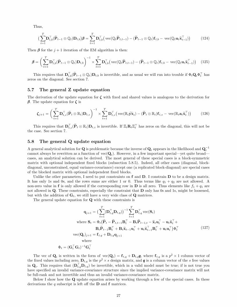
5.8 The general Q update equation

A general analytical solution for Q is problematic because the inverse of Qt appears in the likelihood and Q−1t

cannot always be rewritten as a function of vec(Qt). However, in a few important special—yet quite broad—cases, an analytical solution can be derived. The most general of these special cases is a block-symmetricmatrix with optional independent fixed blocks (subsection 5.8.5). Indeed, all other cases (diagonal, block-diagonal, unconstrained, equal variance-covariance) except one (a replicated block-diagonal) are special casesof the blocked matrix with optional independent fixed blocks.

Unlike the other parameters, I need to put constraints on f and D. I constrain D to be a design matrix.It has only 1s and 0s, and the rows sums are either 1 or 0. Thus terms like q1 + q2 are not allowed. Anon-zero value in f is only allowed if the corresponding row in D is all zero. Thus elements like f1 + q1 arenot allowed in Q. These constraints, especially the constraint that D only has 0s and 1s, might be loosened,but with the addition of Gt, we still have a very wide class of Q matrices.

The general update equation for Q with these constraints is

qj+1 =( T∑t=1

(D>t,qDt,q))−1

T∑t=1

D>t,q vec(St)

where St = Φt(Pt − Pt,t−1B

>t −BtPt−1,t − xtu

>t − utx

>t +

BtPt−1B>t + Btxt−1u

>t + utx

>t−1B

>t + utu

>t

)Φ>t

vec(Qt)j+1 = f t,q + Dt,qqj+1

where

Φt = (G>t Gt)−1G>t

(127)

The vec of Qt is written in the form of vec(Qt) = f t,q + Dt,qqqq, where f t,q is a p2 × 1 column vector ofthe fixed values including zero, Dt,q is the p2 × s design matrix, and qqq is a column vector of the s free values

in Qt. This requires that (D>t,qDt,q) be invertible, which in a valid model must be true; if is not true youhave specified an invalid variance-covariance structure since the implied variance-covariance matrix will notbe full-rank and not invertible and thus an invalid variance-covariance matrix.

Below I show how the Q update equation arises by working through a few of the special cases. In thesederivations the q subscript is left off the D and f matrices.

27

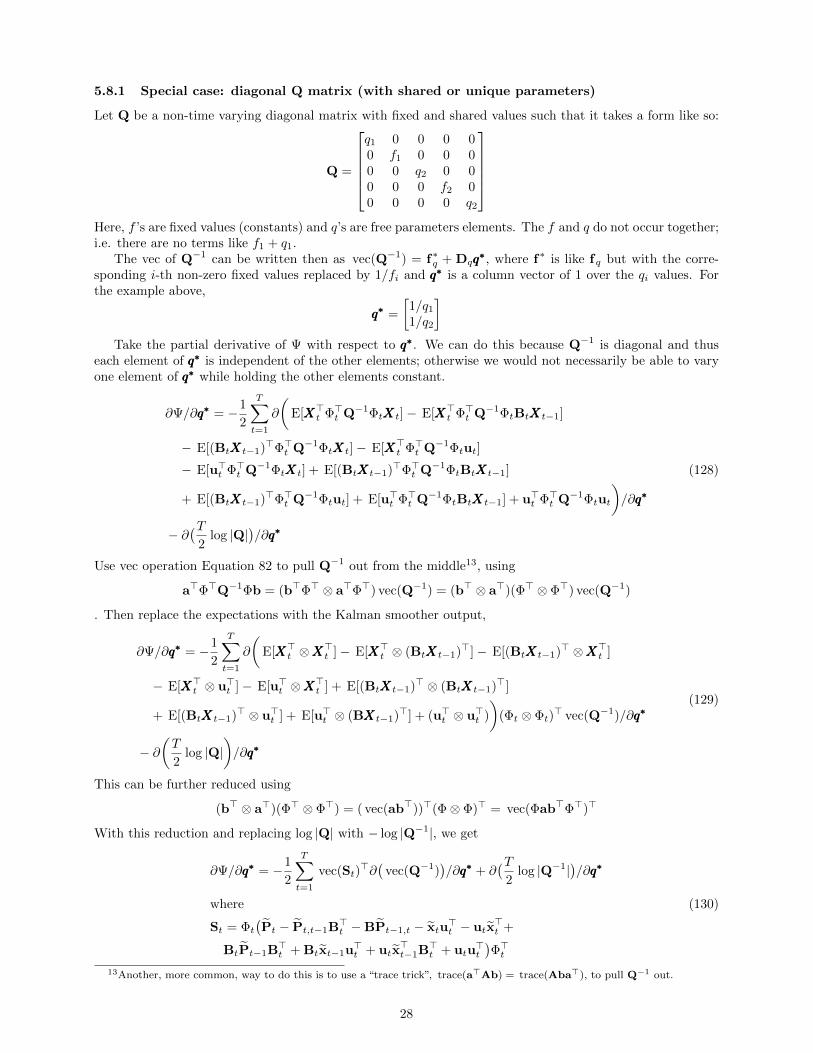
5.8.1 Special case: diagonal Q matrix (with shared or unique parameters)

Let Q be a non-time varying diagonal matrix with fixed and shared values such that it takes a form like so:

Q =

q1 0 0 0 00 f1 0 0 00 0 q2 0 00 0 0 f2 00 0 0 0 q2

Here, f ’s are fixed values (constants) and q’s are free parameters elements. The f and q do not occur together;i.e. there are no terms like f1 + q1.

The vec of Q−1 can be written then as vec(Q−1) = f∗q + Dqq∗q∗q∗, where f∗ is like fq but with the corre-

sponding i-th non-zero fixed values replaced by 1/fi and q∗q∗q∗ is a column vector of 1 over the qi values. Forthe example above,

q∗q∗q∗ =

[1/q1

1/q2

]Take the partial derivative of Ψ with respect to q∗q∗q∗. We can do this because Q−1 is diagonal and thus

each element of q∗q∗q∗ is independent of the other elements; otherwise we would not necessarily be able to varyone element of q∗q∗q∗ while holding the other elements constant.

∂Ψ/∂q∗q∗q∗ = −1

2

T∑t=1

∂

(E[XXX>t Φ>t Q−1ΦtXXXt]− E[XXX>t Φ>t Q−1ΦtBtXXXt−1]

− E[(BtXXXt−1)>Φ>t Q−1ΦtXXXt]− E[XXX>t Φ>t Q−1Φtut]

− E[u>t Φ>t Q−1ΦtXXXt] + E[(BtXXXt−1)>Φ>t Q−1ΦtBtXXXt−1]

+ E[(BtXXXt−1)>Φ>t Q−1Φtut] + E[u>t Φ>t Q−1ΦtBtXXXt−1] + u>t Φ>t Q−1Φtut

)/∂q∗q∗q∗

− ∂(T

2log |Q|

)/∂q∗q∗q∗

(128)

Use vec operation Equation 82 to pull Q−1 out from the middle13, using

a>Φ>Q−1Φb = (b>Φ> ⊗ a>Φ>) vec(Q−1) = (b> ⊗ a>)(Φ> ⊗ Φ>) vec(Q−1)

. Then replace the expectations with the Kalman smoother output,

∂Ψ/∂q∗q∗q∗ = −1

2

T∑t=1

∂

(E[XXX>t ⊗XXX

>t ]− E[XXX>t ⊗ (BtXXXt−1)>]− E[(BtXXXt−1)> ⊗XXX>t ]

− E[XXX>t ⊗ u>t ]− E[u>t ⊗XXX>t ] + E[(BtXXXt−1)> ⊗ (BtXXXt−1)>]

+ E[(BtXXXt−1)> ⊗ u>t ] + E[u>t ⊗ (BXXXt−1)>] + (u>t ⊗ u>t )

)(Φt ⊗ Φt)

> vec(Q−1)/∂q∗q∗q∗

− ∂(T

2log |Q|

)/∂q∗q∗q∗

(129)

This can be further reduced using

(b> ⊗ a>)(Φ> ⊗ Φ>) = ( vec(ab>))>(Φ⊗ Φ)> = vec(Φab>Φ>)>

With this reduction and replacing log |Q| with − log |Q−1|, we get

∂Ψ/∂q∗q∗q∗ = −1

2

T∑t=1

vec(St)>∂(

vec(Q−1))/∂q∗q∗q∗ + ∂

(T2

log |Q−1|)/∂q∗q∗q∗

where

St = Φt(Pt − Pt,t−1B

>t −BPt−1,t − xtu

>t − utx

>t +

BtPt−1B>t + Btxt−1u

>t + utx

>t−1B

>t + utu

>t

)Φ>t

(130)

13Another, more common, way to do this is to use a “trace trick”, trace(a>Ab) = trace(Aba>), to pull Q−1 out.

28

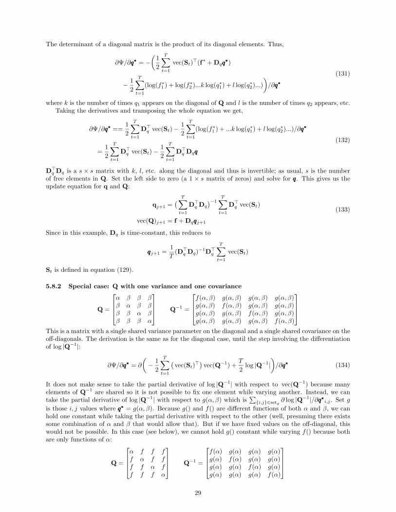
The determinant of a diagonal matrix is the product of its diagonal elements. Thus,

∂Ψ/∂q∗q∗q∗ = −(

1

2

T∑t=1

vec(St)>(f∗ + Dqq

∗q∗q∗)

− 1

2

T∑t=1

(log(f∗1 ) + log(f∗2 )...k log(q∗1) + l log(q∗2)...)

)/∂q∗q∗q∗

(131)

where k is the number of times q1 appears on the diagonal of Q and l is the number of times q2 appears, etc.Taking the derivatives and transposing the whole equation we get,

∂Ψ/∂q∗q∗q∗ ==1

2

T∑t=1

D>q vec(St)−1

2

T∑t=1

(log(f∗1 ) + ...k log(q∗1) + l log(q∗2)...)/∂q∗q∗q∗

=1

2

T∑t=1

D>q vec(St)−1

2

T∑t=1

D>q Dqqqq

(132)

D>q Dq is a s × s matrix with k, l, etc. along the diagonal and thus is invertible; as usual, s is the numberof free elements in Q. Set the left side to zero (a 1 × s matrix of zeros) and solve for qqq. This gives us theupdate equation for q and Q:

qj+1 =( T∑t=1

D>q Dq

)−1T∑t=1

D>q vec(St)

vec(Q)j+1 = f + Dqqqqj+1

(133)

Since in this example, Dq is time-constant, this reduces to

qqqj+1 =1

T(D>q Dq)

−1D>q

T∑t=1

vec(St)

St is defined in equation (129).

5.8.2 Special case: Q with one variance and one covariance

Q =

α β β ββ α β ββ β α ββ β β α

Q−1 =

f(α, β) g(α, β) g(α, β) g(α, β)g(α, β) f(α, β) g(α, β) g(α, β)g(α, β) g(α, β) f(α, β) g(α, β)g(α, β) g(α, β) g(α, β) f(α, β)

This is a matrix with a single shared variance parameter on the diagonal and a single shared covariance on theoff-diagonals. The derivation is the same as for the diagonal case, until the step involving the differentiationof log |Q−1|:

∂Ψ/∂q∗q∗q∗ = ∂

(− 1

2

T∑t=1

(vec(St)

>) vec(Q−1) +T

2log |Q−1|

)/∂q∗q∗q∗ (134)

It does not make sense to take the partial derivative of log |Q−1| with respect to vec(Q−1) because manyelements of Q−1 are shared so it is not possible to fix one element while varying another. Instead, we cantake the partial derivative of log |Q−1| with respect to g(α, β) which is

∑i,j∈setg

∂ log |Q−1|/∂q∗q∗q∗i,j . Set g

is those i, j values where q∗q∗q∗ = g(α, β). Because g() and f() are different functions of both α and β, we canhold one constant while taking the partial derivative with respect to the other (well, presuming there existssome combination of α and β that would allow that). But if we have fixed values on the off-diagonal, thiswould not be possible. In this case (see below), we cannot hold g() constant while varying f() because bothare only functions of α:

Q =

α f f ff α f ff f α ff f f α

Q−1 =

f(α) g(α) g(α) g(α)g(α) f(α) g(α) g(α)g(α) g(α) f(α) g(α)g(α) g(α) g(α) f(α)

29

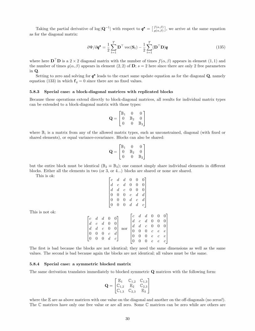
Taking the partial derivative of log |Q−1| with respect to q∗q∗q∗ =[ f(α,β)g(α,β)

], we arrive at the same equation

as for the diagonal matrix:

∂Ψ/∂q∗q∗q∗ =1

2

T∑t=1

D> vec(St)−1

2

T∑t=1

(D>D)qqq (135)

where here D>D is a 2× 2 diagonal matrix with the number of times f(α, β) appears in element (1, 1) andthe number of times g(α, β) appears in element (2, 2) of D; s = 2 here since there are only 2 free parametersin Q.

Setting to zero and solving for q∗q∗q∗ leads to the exact same update equation as for the diagonal Q, namelyequation (133) in which fq = 0 since there are no fixed values.

5.8.3 Special case: a block-diagonal matrices with replicated blocks

Because these operations extend directly to block-diagonal matrices, all results for individual matrix typescan be extended to a block-diagonal matrix with those types:

Q =

B1 0 00 B2 00 0 B3

where Bi is a matrix from any of the allowed matrix types, such as unconstrained, diagonal (with fixed orshared elements), or equal variance-covariance. Blocks can also be shared:

Q =

B1 0 00 B2 00 0 B2

but the entire block must be identical (B2 ≡ B3); one cannot simply share individual elements in differentblocks. Either all the elements in two (or 3, or 4...) blocks are shared or none are shared.

This is ok: c d d 0 0 0d c d 0 0 0d d c 0 0 00 0 0 c d d0 0 0 d c d0 0 0 d d c

This is not ok:

c d d 0 0d c d 0 0d d c 0 00 0 0 c d0 0 0 d c

nor

c d d 0 0 0d c d 0 0 0d d c 0 0 00 0 0 c e e0 0 0 e c e0 0 0 e e c

The first is bad because the blocks are not identical; they need the same dimensions as well as the samevalues. The second is bad because again the blocks are not identical; all values must be the same.

5.8.4 Special case: a symmetric blocked matrix

The same derivation translates immediately to blocked symmetric Q matrices with the following form:

Q =

E1 C1,2 C1,3

C1,2 E2 C2,3

C1,3 C2,3 E3

where the E are as above matrices with one value on the diagonal and another on the off-diagonals (no zeros!).The C matrices have only one free value or are all zero. Some C matrices can be zero while are others are

30

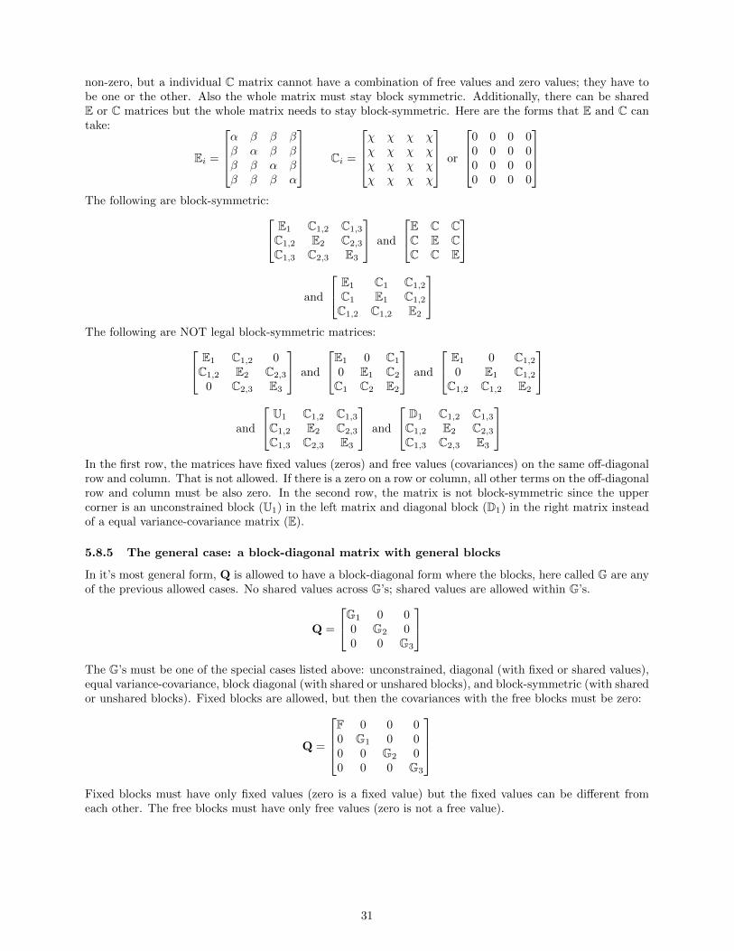
non-zero, but a individual C matrix cannot have a combination of free values and zero values; they have tobe one or the other. Also the whole matrix must stay block symmetric. Additionally, there can be sharedE or C matrices but the whole matrix needs to stay block-symmetric. Here are the forms that E and C cantake:

Ei =

α β β ββ α β ββ β α ββ β β α

Ci =

χ χ χ χχ χ χ χχ χ χ χχ χ χ χ

or

0 0 0 00 0 0 00 0 0 00 0 0 0

The following are block-symmetric: E1 C1,2 C1,3

C1,2 E2 C2,3

C1,3 C2,3 E3

and

E C CC E CC C E

and

E1 C1 C1,2

C1 E1 C1,2

C1,2 C1,2 E2

The following are NOT legal block-symmetric matrices: E1 C1,2 0

C1,2 E2 C2,3

0 C2,3 E3

and

E1 0 C1

0 E1 C2

C1 C2 E2

and

E1 0 C1,2

0 E1 C1,2

C1,2 C1,2 E2

and

U1 C1,2 C1,3

C1,2 E2 C2,3

C1,3 C2,3 E3

and

D1 C1,2 C1,3

C1,2 E2 C2,3

C1,3 C2,3 E3

In the first row, the matrices have fixed values (zeros) and free values (covariances) on the same off-diagonalrow and column. That is not allowed. If there is a zero on a row or column, all other terms on the off-diagonalrow and column must be also zero. In the second row, the matrix is not block-symmetric since the uppercorner is an unconstrained block (U1) in the left matrix and diagonal block (D1) in the right matrix insteadof a equal variance-covariance matrix (E).

5.8.5 The general case: a block-diagonal matrix with general blocks

In it’s most general form, Q is allowed to have a block-diagonal form where the blocks, here called G are anyof the previous allowed cases. No shared values across G’s; shared values are allowed within G’s.

Q =

G1 0 00 G2 00 0 G3

The G’s must be one of the special cases listed above: unconstrained, diagonal (with fixed or shared values),equal variance-covariance, block diagonal (with shared or unshared blocks), and block-symmetric (with sharedor unshared blocks). Fixed blocks are allowed, but then the covariances with the free blocks must be zero:

Q =

F 0 0 00 G1 0 00 0 G2 00 0 0 G3

Fixed blocks must have only fixed values (zero is a fixed value) but the fixed values can be different fromeach other. The free blocks must have only free values (zero is not a free value).

31

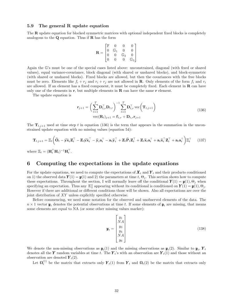
5.9 The general R update equation

The R update equation for blocked symmetric matrices with optional independent fixed blocks is completelyanalogous to the Q equation. Thus if R has the form

R =

F 0 0 00 G1 0 00 0 G2 00 0 0 G3

Again the G’s must be one of the special cases listed above: unconstrained, diagonal (with fixed or sharedvalues), equal variance-covariance, block diagonal (with shared or unshared blocks), and block-symmetric(with shared or unshared blocks). Fixed blocks are allowed, but then the covariances with the free blocksmust be zero. Elements like fi + rj and ri + rj are not allowed in R. Only elements of the form fi and riare allowed. If an element has a fixed component, it must be completely fixed. Each element in R can haveonly one of the elements in r, but multiple elements in R can have the same r element.

The update equation is

rj+1 =

( T∑t=1

D>t,rDt,r

)−1 T∑t=1

D>t,r vec

(Tt,j+1

)vec(Rt)j+1 = f t,r + Dt,rrj+1

(136)

The Tt,j+1 used at time step t in equation (136) is the term that appears in the summation in the uncon-strained update equation with no missing values (equation 54):

Tt,j+1 = Ξt

(Ot − yxtZ

>t − Ztyx

>t − yta

>t − aty

>t + ZtPtZ

>t + Ztxta

>t + atx

>t Z>t + ata

>t

)Ξ>t (137)

where Ξt = (H>t Ht)−1H>t .

6 Computing the expectations in the update equations

For the update equations, we need to compute the expectations of XXXt and YYY t and their products conditionedon 1) the observed data YYY (1) = yyy(1) and 2) the parameters at time t, Θj . This section shows how to computethese expectations. Throughout the section, I will normally leave off the conditional YYY (1) = yyy(1),Θj whenspecifying an expectation. Thus any E[] appearing without its conditional is conditioned on YYY (1) = yyy(1),Θj .However if there are additional or different conditions those will be shown. Also all expectations are over thejoint distribution of XY unless explicitly specified otherwise.

Before commencing, we need some notation for the observed and unobserved elements of the data. Then× 1 vector yyyt denotes the potential observations at time t. If some elements of yyyt are missing, that meanssome elements are equal to NA (or some other missing values marker):

yyyt =

y1

NAy3

y4

NAy6

(138)

We denote the non-missing observations as yyyt(1) and the missing observations as yyyt(2). Similar to yyyt, YYY tdenotes all the YYY random variables at time t. The YYY t’s with an observation are YYY t(1) and those without anobservation are denoted YYY t(2).

Let Ω(1)t be the matrix that extracts only YYY t(1) from YYY t and Ωt(2) be the matrix that extracts only

32

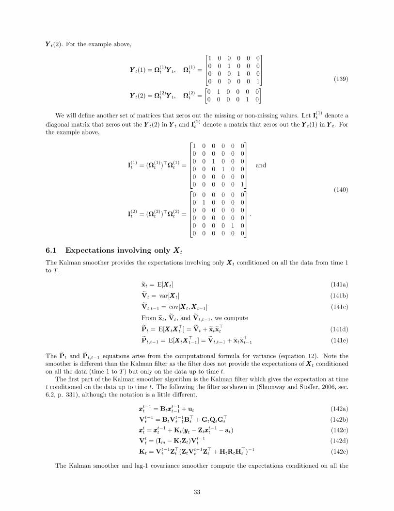
YYY t(2). For the example above,

YYY t(1) = Ω(1)t YYY t, Ω

(1)t =

1 0 0 0 0 00 0 1 0 0 00 0 0 1 0 00 0 0 0 0 1

YYY t(2) = Ω

(2)t YYY t, Ω

(2)t =

[0 1 0 0 0 00 0 0 0 1 0

] (139)

We will define another set of matrices that zeros out the missing or non-missing values. Let I(1)t denote a

diagonal matrix that zeros out the YYY t(2) in YYY t and I(2)t denote a matrix that zeros out the YYY t(1) in YYY t. For

the example above,

I(1)t = (Ω

(1)t )>Ω

(1)t =

1 0 0 0 0 00 0 0 0 0 00 0 1 0 0 00 0 0 1 0 00 0 0 0 0 00 0 0 0 0 1

and

I(2)t = (Ω

(2)t )>Ω

(2)t =

0 0 0 0 0 00 1 0 0 0 00 0 0 0 0 00 0 0 0 0 00 0 0 0 1 00 0 0 0 0 0

.(140)

6.1 Expectations involving only XXX t

The Kalman smoother provides the expectations involving only XXXt conditioned on all the data from time 1to T .

xt = E[XXXt] (141a)

Vt = var[XXXt] (141b)

Vt,t−1 = cov[XXXt,XXXt−1] (141c)

From xt, Vt, and Vt,t−1, we compute

Pt = E[XXXtXXX>t ] = Vt + xtx

>t (141d)

Pt,t−1 = E[XXXtXXX>t−1] = Vt,t−1 + xtx

>t−1 (141e)

The Pt and Pt,t−1 equations arise from the computational formula for variance (equation 12). Note thesmoother is different than the Kalman filter as the filter does not provide the expectations of XXXt conditionedon all the data (time 1 to T ) but only on the data up to time t.

The first part of the Kalman smoother algorithm is the Kalman filter which gives the expectation at timet conditioned on the data up to time t. The following the filter as shown in (Shumway and Stoffer, 2006, sec.6.2, p. 331), although the notation is a little different.

xxxt−1t = Btxxx

t−1t−1 + ut (142a)

Vt−1t = BtV

t−1t−1B

>t + GtQtG

>t (142b)

xxxtt = xxxt−1t + Kt(yyyt − Ztxxx

t−1t − at) (142c)

Vtt = (Im −KtZt)V

t−1t (142d)

Kt = Vt−1t Z>t (ZtV

t−1t Z>t + HtRtH

>t )−1 (142e)

The Kalman smoother and lag-1 covariance smoother compute the expectations conditioned on all the

33

data, 1 to T :

xxxTt−1 = xxxt−1t−1 + Jt−1(xxxTt − xxxt−1

t ) (143a)

VTt−1 = Vt−1

t−1 + Jt−1(VTt −Vt−1

t )J>t (143b)

Jt−1 = Vt−1t−1B

>t (Vt−1

t )−1 (143c)

(143d)

VTT,T−1 = (I−KTZT )BTVT−1

T−1 (143e)

VTt−1,t−2 = Vt−1

t−1J>t−2 + Jt−1((VT

t,t−1 −BtVt−1t−1))J>t−2 (143f)

The classic Kalman smoother is an algorithm to compute these expectations conditioned on no missingvalues in yyy. However, the algorithm can be easily modified to give the expected values of XXX conditioned onthe incomplete data, YYY (1) = yyy(1) (Shumway and Stoffer, 2006, sec. 6.4, eqn 6.78, p. 348). In this case, theusual filter and smoother equations are used with the following modifications to the parameters and dataused in the equations. If the i-th element of yyyt is missing, zero out the i-th rows in yyyt, a and Z. Thus if the2nd and 5th elements of yyyt are missing,

yyy∗t =

y1

0y3

y4

0y6

, a∗t =

a1

0a3

a4

0a6

, Z∗t =

z1,1 z1,2 ...0 0 ...z3,1 z3,2 ...z4,1 z4,2 ...0 0 ...z6,1 z6,2 ...

(144)

The Rt parameter used in the filter equations is also modified. We need to zero out the covariancesbetween the non-missing, yyyt(1), and missing, yyyt(2), data. For the example above, if

Rt = HtRH>t =

r1,1 r1,2 r1,3 r1,4 r1,5 r1,6

r2,1 r2,2 r2,3 r2,4 r2,5 r2,6

r3,1 r3,2 r3,3 r3,4 r3,5 r3,6

r4,1 r4,2 r4,3 r4,4 r4,5 r4,6

r5,1 r5,2 r5,3 r5,4 r5,5 r5,6

r6,1 r6,2 r6,3 r6,4 r6,5 r6,6

(145)

then the Rt we use at time t, will have zero covariances between the non-missing elements 1,3,4,6 and themissing elements 2,5:

R∗t =

r1,1 0 r1,3 r1,4 0 r1,6

0 r2,2 0 0 r2,5 0r3,1 0 r3,3 r3,4 0 r3,6

r4,1 0 r4,3 r4,4 0 r4,6

0 r5,2 0 0 r5,5 0r6,1 0 r6,3 r6,4 0 r6,6

(146)

Thus, the data and parameters used in the filter and smoother equations are

yyy∗t = I(1)t yyyt

a∗t = I(1)t at

Z∗t = I(1)t Zt

R∗t = I(1)t RtI

(1)t + I

(2)t RtI

(2)t

(147)

a∗t , Z∗t and R∗t only are used in the Kalman filter and smoother. They are not used in the EM updateequations. However when coding the algorithm, it is convenient to replace the NAs (or whatever the missingvalues placeholder is) in yyyt with zero so that there is not a problem with NAs appearing in the computations.

34

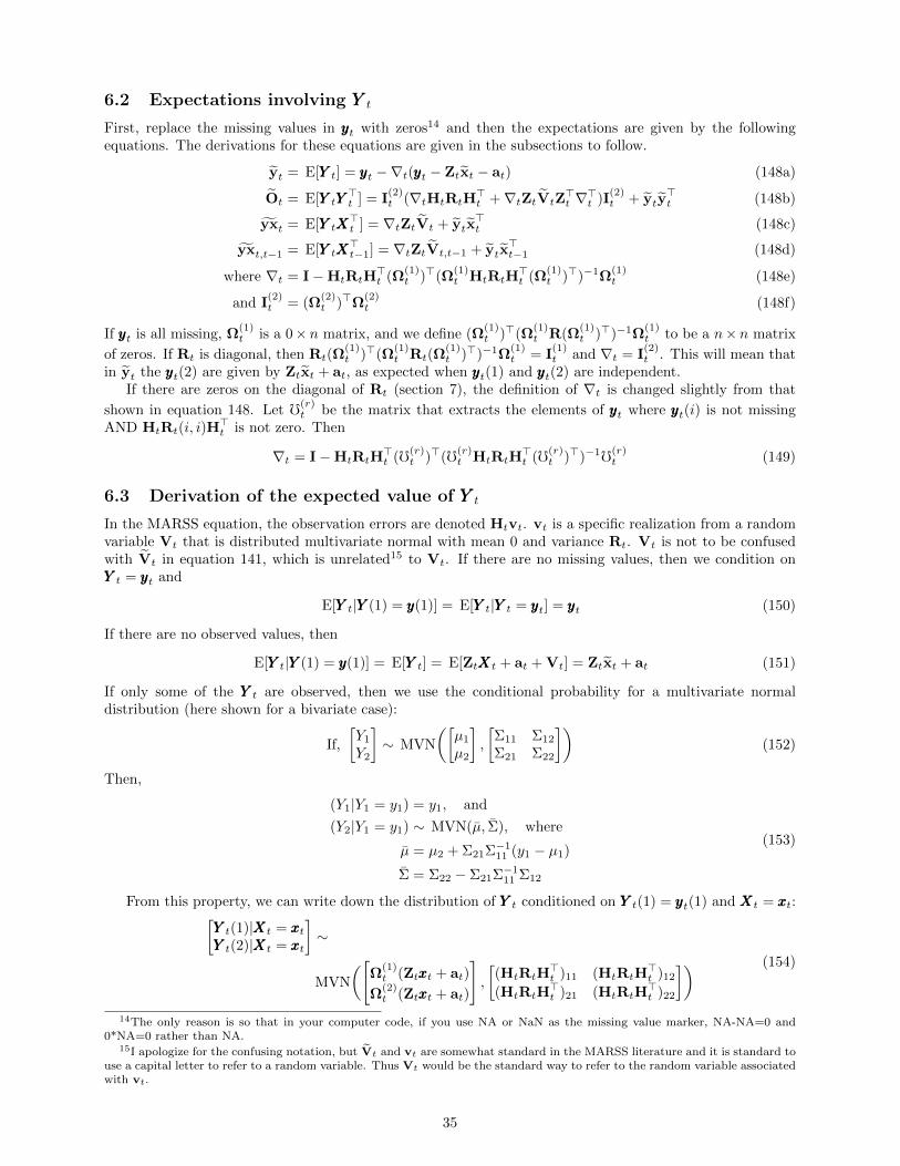
6.2 Expectations involving YYY t

First, replace the missing values in yyyt with zeros14 and then the expectations are given by the followingequations. The derivations for these equations are given in the subsections to follow.

yt = E[YYY t] = yyyt −∇t(yyyt − Ztxt − at) (148a)

Ot = E[YYY tYYY>t ] = I

(2)t (∇tHtRtH

>t +∇tZtVtZ

>t ∇>t )I

(2)t + yty

>t (148b)

yxt = E[YYY tXXX>t ] = ∇tZtVt + ytx

>t (148c)

yxt,t−1 = E[YYY tXXX>t−1] = ∇tZtVt,t−1 + ytx

>t−1 (148d)

where ∇t = I−HtRtH>t (Ω

(1)t )>(Ω

(1)t HtRtH

>t (Ω

(1)t )>)−1Ω

(1)t (148e)

and I(2)t = (Ω

(2)t )>Ω

(2)t (148f)

If yyyt is all missing, Ω(1)t is a 0× n matrix, and we define (Ω

(1)t )>(Ω

(1)t R(Ω

(1)t )>)−1Ω

(1)t to be a n× n matrix

of zeros. If Rt is diagonal, then Rt(Ω(1)t )>(Ω

(1)t Rt(Ω

(1)t )>)−1Ω

(1)t = I

(1)t and ∇t = I

(2)t . This will mean that

in yt the yyyt(2) are given by Ztxt + at, as expected when yyyt(1) and yyyt(2) are independent.If there are zeros on the diagonal of Rt (section 7), the definition of ∇t is changed slightly from that

shown in equation 148. Let f(r)t be the matrix that extracts the elements of yyyt where yyyt(i) is not missing

AND HtRt(i, i)H>t is not zero. Then

∇t = I−HtRtH>t (f(r)

t )>(f(r)t HtRtH

>t (f(r)

t )>)−1f(r)t (149)

6.3 Derivation of the expected value of YYY t

In the MARSS equation, the observation errors are denoted Htvt. vt is a specific realization from a randomvariable Vt that is distributed multivariate normal with mean 0 and variance Rt. Vt is not to be confusedwith Vt in equation 141, which is unrelated15 to Vt. If there are no missing values, then we condition onYYY t = yyyt and

E[YYY t|YYY (1) = yyy(1)] = E[YYY t|YYY t = yyyt] = yyyt (150)

If there are no observed values, then

E[YYY t|YYY (1) = yyy(1)] = E[YYY t] = E[ZtXXXt + at + Vt] = Ztxt + at (151)

If only some of the YYY t are observed, then we use the conditional probability for a multivariate normaldistribution (here shown for a bivariate case):

If,

[Y1

Y2

]∼ MVN

([µ1

µ2

],

[Σ11 Σ12

Σ21 Σ22

])(152)

Then,

(Y1|Y1 = y1) = y1, and

(Y2|Y1 = y1) ∼ MVN(µ, Σ), where

µ = µ2 + Σ21Σ−111 (y1 − µ1)

Σ = Σ22 − Σ21Σ−111 Σ12

(153)

From this property, we can write down the distribution of YYY t conditioned on YYY t(1) = yyyt(1) and XXXt = xxxt:[YYY t(1)|XXXt = xxxtYYY t(2)|XXXt = xxxt

]∼

MVN

([Ω

(1)t (Ztxxxt + at)

Ω(2)t (Ztxxxt + at)

],

[(HtRtH

>t )11 (HtRtH

>t )12

(HtRtH>t )21 (HtRtH

>t )22

]) (154)

14The only reason is so that in your computer code, if you use NA or NaN as the missing value marker, NA-NA=0 and0*NA=0 rather than NA.

15I apologize for the confusing notation, but Vt and vt are somewhat standard in the MARSS literature and it is standard touse a capital letter to refer to a random variable. Thus Vt would be the standard way to refer to the random variable associatedwith vt.

35

Thus,

(YYY t(1)|YYY t(1) = yyyt(1),XXXt = xxxt) = Ω(1)t yyyt and

(YYY t(2)|YYY t(1) = yyyt(1),XXXt = xxxt) ∼ MVN(µ, Σ) where

µ = Ω(2)t (Ztxxxt + at) + Rt,21(Rt,11)−1Ω

(1)t (yyyt − Ztxxxt − at)

Σ = Rt,22 − Rt,21(Rt,11)−1Rt,12

Rt = HtRtH>t

(155)

Note that since we are conditioning on XXXt = xxxt, we can replace YYY by YYY t in the conditional:

E[YYY t|YYY (1) = yyy(1),XXXt = xxxt] = E[YYY t|YYY t(1) = yyyt(1),XXXt = xxxt].

From this and the distributions in equation (155), we can write down yt = E[YYY t|YYY (1) = yyy(1),Θj ]:

yt = EXY [YYY t|YYY (1) = yyy(1)]

=

∫xxxt

∫yyyt

yyytf(yyyt|yyyt(1),xxxt)dyyytf(xxxt)dxxxt

= EX [ EY |x[YYY t|YYY t(1) = yyyt(1),XXXt = xxxt]]

= EX [yyyt −∇t(yyyt − ZtXXXt − at)]

= yyyt −∇t(yyyt − Ztxt − at)

where ∇t = I− Rt(Ω(1)t )>(Rt,11)−1Ω

(1)t

(156)

(Ω(1)t )>(Rt,11)−1Ω

(1)t is a n×n matrix with 0s in the non-(11) positions. If the k-th element of yyyt is observed,

then k-th row and column of ∇t will be zero. Thus if there are no missing values at time t, ∇t = I− I = 0.If there are no observed values at time t, ∇t will reduce to I.

6.4 Derivation of the expected value of YYY tYYY>t

The following outlines a16 derivation. If there are no missing values, then we condition on YYY t = yyyt and

E[YYY tYYY>t |YYY (1) = yyy(1)] = E[YYY tYYY

>t |YYY t = yyyt]

= yyytyyy>t .

(157)

If there are no observed values at time t, then

E[YYY tYYY>t ]

= var[ZtXXXt + at + HtVt] + E[ZtXXXt + at + HtVt] E[ZtXXXt + at + HtVt]>

= var[Vt] + var[ZtXXXt] + ( E[ZtXXXt + at] + E[HtVt])( E[ZtXXXt + at] + E[HtVt])>

= Rt + ZtVtZ>t + (Ztxt + at)(Ztxt + at)

>

(158)

When only some of the YYY t are observed, we use again the conditional probability of a multivariate normal(equation 152). From this property, we know that

varY |x[YYY t(2)YYY t(2)>|YYY t(1) = yyyt(1),XXXt = xxxt] = Rt,22 − Rt,21(Rt,11)−1Rt,12,

varY |x[YYY t(1)|YYY t(1) = yyyt(1),XXXt = xxxt] = 0

and covY |x[YYY t(1),YYY t(2)|YYY t(1) = yyyt(1),XXXt = xxxt] = 0

Thus varY |x[YYY t|YYY t(1) = yyyt(1),XXXt = xxxt]

= (Ω(2)t )>(Rt,22 − Rt,21(Rt,11)−1Rt,12)Ω

(2)t

= (Ω(2)t )>(Ω

(2)t Rt(Ω

(2)t )> −Ω

(2)t Rt(Ω

(1)t )>(Rt,11)−1Ω

(1)t Rt(Ω

(2)t )>)Ω

(2)t

= I(2)t (Rt − Rt(Ω

(1)t )>(Rt,11)−1Ω

(1)t Rt)I

(2)t

= I(2)t ∇tRtI

(2)t

(159)

16The following derivations are painfully ugly, but appear to work. There are surely more elegant ways to do this; at least,there must be more elegant notations.

36

The I(2)t bracketing both sides is zero-ing out the rows and columns corresponding to the yyyt(1) values.

Now we can compute the EXY [YYY tYYY>t |YYY (1) = yyy(1)]. The subscripts are added to the E to emphasize that

we are breaking the multivariate expectation into an inner and outer expectation.

Ot = EXY [YYY tYYY>t |YYY (1) = yyy(1)] = EX [ EY |x[YYY tYYY

>t |YYY t(1) = yyyt(1),XXXt = xxxt]]

= EX[

varY |x[YYY t|YYY t(1) = yyyt(1),XXXt = xxxt]

+ EY |x[YYY t|YYY t(1) = yyyt(1),XXXt = xxxt] EY |x[YYY t|YYY t(1) = yyyt(1),XXXt = xxxt]>]

= EX [I(2)t ∇tRtI

(2)t ] + EX [(yyyt −∇t(yyyt − ZtXXXt − at))(yyyt −∇t(yyyt − ZtXXXt − at))

>]

= I(2)t ∇tRtI

(2)t + varX

[yyyt −∇t(yyyt − ZtXXXt − at)

]+ EX [yyyt −∇t(yyyt − ZtXXXt − at)] EX [yyyt −∇t(yyyt − ZtXXXt − at)]

>

= I(2)t ∇tRtI

(2)t + I

(2)t ∇tZtVtZ

>t ∇>t I

(2)t + yty

>t

(160)

Thus,

Ot = I(2)t (∇tRt +∇tZtVtZ

>t ∇>t )I

(2)t + yty

>t (161)

6.5 Derivation of the expected value of YYY tXXX>t

If there are no missing values, then we condition on YYY t = yyyt and

E[YYY tXXX>t |YYY (1) = yyy(1)] = yyyt E[XXX>t ] = yyytx

>t (162)

If there are no observed values at time t, then

E[YYY tXXX>t |YYY (1) = yyy(1)]

= E[(ZtXXXt + at + Vt)XXX>t ]

= E[ZtXXXtXXX>t + atXXX

>t + VtXXX

>t ]

= ZtPt + atx>t + cov[Vt,XXXt] + E[Vt] E[XXXt]

>

= ZtPt + atx>t

(163)

Note that Vt and XXXt are independent (equation 1). E[Vt] = 0 and cov[Vt,XXXt] = 0.Now we can compute the EXY [YYY tXXX

>t |YYY (1) = yyy(1)].

yxt = EXY [YYY tXXX>t |YYY (1) = yyy(1)]

= cov[YYY t,XXXt|YYY t(1) = yyyt(1)] + EXY [YYY t|YYY (1) = yyy(1)] EXY [XXX>t |YYY (1) = yyy(1)]>

= cov[yyyt −∇t(yyyt − ZtXXXt − at) + V∗t ,XXXt] + ytx>t

= cov[yyyt,XXXt]− cov[∇tyyyt,XXXt] + cov[∇tZtXXXt,XXXt] + cov[∇tat,XXXt]

+ cov[V∗t ,XXXt] + ytx>t

= 0− 0 +∇tZtVt + 0 + 0 + ytx>t

= ∇tZtVt + ytx>t

(164)

This uses the computational formula for covariance: E[YYYXXX>] = cov[YYY ,XXX] + E[YYY ] E[XXX]>. V∗t is a ran-dom variable with mean 0 and variance Rt,22 − Rt,21(Rt,11)−1Rt,12 from equation (155). V∗t and XXXt are

independent of each other, thus cov[V∗t ,XXX>t ] = 0.

37

6.6 Derivation of the expected value of YYY tXXX>t−1

The derivation of E[YYY tXXX>t−1] is similar to the derivation of E[YYY tXXX

>t−1]:

yxt = EXY [YYY tXXX>t−1|YYY (1) = yyy(1)]

= cov[YYY t,XXXt−1|YYY t(1) = yyyt(1)] + EXY [YYY t|YYY (1) = yyy(1)] EXY [XXX>t−1|YYY (1) = yyy(1)]>

= cov[yyyt −∇t(yyyt − ZtXXXt − at) + V∗t ,XXXt−1] + ytx>t−1

= cov[yyyt,XXXt−1]− cov[∇tyyyt,XXXt−1] + cov[∇tZtXXXt,XXXt−1]

+ cov[∇tat,XXXt−1] + cov[V∗t ,XXXt−1] + ytx>t−1

= 0− 0 +∇tZtVt,t−1 + 0 + 0 + ytx>t−1

= ∇tZtVt,t−1 + ytx>t−1

(165)

7 Degenerate variance models

It is possible that the model has deterministic and probabilistic elements; mathematically this means thateither Gt, Ht or F have all zero rows, and this means that some of the observation or state processes aredeterministic. Such models often arise when a MAR-p is put into MARSS-1 form. Assuming the model issolvable (one solution and not over-determined), we can modify the Kalman smoother and EM algorithm tohandle models with deterministic elements.

The motivation behind the degenerate variance modification is that we want to use one set of EM updateequations for all models in the MARSS class—regardless of whether they are partially or fully degenerate.The difficulties arise in getting the u and ξ update equations. If we were to fix these or make ξ stochastic(a fixed mean and fixed variance), most of the trouble in this section could be avoided. However, fixingξ or making it stochastic is putting a prior on it and placing a prior on the variance-covariance structureof ξ that conflicts logically with the model is often both unavoidable (since the correct variance-covariancestructure depends on the parameters you are trying to estimate) and disastrous to one’s estimation althoughthe problem is often difficult to detect especially with long time series. Many papers have commented on thissubtle problem. So, we want to be able to estimate ξ so we do not have to specify Λ (because we removeit from the model). Note that in a univariate xxx model (one state), Λ is just a variance so we do not runinto this trouble. The problems arise when xxx is multivariate (>1 state) and then we have to deal with thevariance-covariance structure of the initial states.

7.1 Rewriting the state and observation models for degenerate variance systems

Let’s start with an example:

Rt =

[1 .2.2 1

]and Ht =

1 00 00 1

(166)

Let Ω+t,r be a p×n matrix that extracts the p non-zero rows from Ht. The diagonal matrix (Ω+

t,r)>Ω+

t,r ≡ I+t,r

is a diagonal matrix that can zero out the Ht zero rows in any n row matrix.

Ω+t,r =

[1 0 00 0 1

]I+t,r = (Ω+

t,r)>Ω+

t,r =

1 0 00 0 00 0 1

yyy+t = Ω+

t,ryyyt

(167)

Let Ω(0)t,r be a (n− p)× n matrix that extracts the n− p zero rows from Ht. For the example above,

Ω(0)t,r =

[0 1 0

]I(0)t,r = (Ω

(0)t,r )>Ω

(0)t,r =

0 0 00 1 00 0 0

yyy

(0)t = Ω

(0)t,ryyyt

(168)

38

Similarly, Ω+t,q extracts the non-zero rows from Gt and Ω

(0)t,q extracts the zero rows. I+

t,q and I(0)t,q are defined

similarly.Using these definitions, we can rewrite the state process part of the MARSS model by separating out the

deterministic parts:

xxx(0)t = Ω

(0)t,qxxxt = Ω

(0)t,q (Btxxxt−1 + ut)

xxx+t = Ω+

t,qxxxt = Ω+t,q(Btxxxt−1 + ut + Gtwt)

w+t ∼ MVN(0,Qt)

xxx0 ∼ MVN(ξ,Λ)

(169)

Similarly, we can rewrite the observation process part of the MARSS model by separating out the parts withno observation error:

yyy(0)t = Ω

(0)t,ryyyt = Ω

(0)t,r (Ztxxxt + at)

= Ω(0)t,r (ZtI

+t,qxxxt + ZtI

(0)t,qxxxt + at)

yyy+t = Ω+

t,ryyyt = Ω+t,r(Ztxxxt + at + Htvt)

= Ω+t,r(ZtI

+t,qxxxt + ZtI

(0)t,qxxxt + at + Htvt)

v+t ∼ MVN(0,Rt)

(170)

I am treating Λ as fully stochastic for this example, but in general F might have 0 rows.In order for this to be solvable using an EM algorithm with the Kalman filter, we require that no estimated

B or u elements appear in the equation for yyy(0)t . Since the yyy

(0)t do not appear in the likelihood function (since

H(0)t = 0), yyy

(0)t would not affect the estimate for the parameters appearing in the yyy

(0)t equation. This

translates to the following constraints, (11×m ⊗ Ω(0)t,rZtI

(0)t,q )Dt,b is all zeros and Ω

(0)t,rZtI

(0)t,qDu is all zeros.

Also notice that Ω(0)t,rZt and Ω

(0)t,rat appear in the yyy(0) equation and not in the yyy+ equation. This means that

Ω(0)t,rZt and Ω

(0)t,rat must be only fixed terms.

In summary, the degenerate model becomes

xxx(0)t = B

(0)t xxxt−1 + u

(0)t

xxx+t = B+

t xxxt−1 + u+t + G+

t wt

wt ∼ MVN(0,Qt)

xxx0 ∼ MVN(ξ,Λ)

yyy(0)t = Z(0)I+

q xxxt + Z(0)I(0)q xxxt + a

(0)t

yyy+t = Z+

t xxxt + a+t H+

t vt

= Z+t I+

q xxxt + Z+t I(0)

q xxxt + a+t + H+

t vt

vt ∼ MVN(0,R)

(171)

where B(0)t = Ω

(0)t,qBt and B+

t = Ω+t,qBt so that B

(0)t are the rows of Bt corresponding to the zero rows of Gt

and B+t are the rows of Bt corresponding to non-zero rows of Gt. The other parameters are similarly defined:

u(0)t = Ω

(0)t,qut and u+

t = Ω+t,qut, Z

(0)t = Ω

(0)t,rZt and Z+

t = Ω+t,rZt, and a

(0)t = Ω

(0)t,rat and a+

t = Ω+t,rat.

7.2 Identifying the fully deterministic xxx rows

To derive EM update equations, we need to take the derivative of the expected log-likelihood holding every-thing but the parameter of interest constant. If there are deterministic xxxt rows, then we cannot hold theseconstant and do this partial differentiation with respect to the state parameters. We need to identify these xxxtrows and remove them from the likelihood function by rewriting them in terms of only the state parameters.For this derivation, I am going to make the simplifying assumption that the locations of the 0 rows in Gt

and Ht are time-invariant. This is not strictly necessary, but simplifies the algebra greatly.For the deterministic xxxt rows, the process equation is xxxt = Btxxxt−1 + ut, with the wt term left off. When

we do the partial differentiation step in deriving the EM update equation for u, B or ξ, we will need to take

39

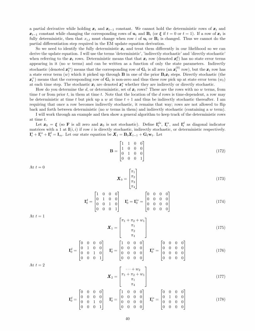
a partial derivative while holding xxxt and xxxt−1 constant. We cannot hold the deterministic rows of xxxt andxxxt−1 constant while changing the corresponding rows of ut and Bt (or ξ if t = 0 or t = 1). If a row of xxxt isfully deterministic, then that xi,t must change when row i of ut or Bt is changed. Thus we cannot do thepartial differentiation step required in the EM update equation derivation.

So we need to identify the fully deterministic xxxt and treat them differently in our likelihood so we canderive the update equation. I will use the terms ’deterministic’, ’indirectly stochastic’ and ’directly stochastic’when referring to the xxxt rows. Deterministic means that that xxxt row (denoted xxxdt ) has no state error termsappearing in it (no w terms) and can be written as a function of only the state parameters. Indirectly

stochastic (denoted xxxist ) means that the corresponding row of Gt is all zero (an xxx(0)t row), but the xxxt row has

a state error term (w) which it picked up through B in one of the prior Btxxxt steps. Directly stochastic (thexxx+t ) means that the corresponding row of Gt is non-zero and thus these row pick up at state error term (wt)

at each time step. The stochastic xxxt are denoted xxxst whether they are indirectly or directly stochastic.How do you determine the d, or deterministic, set of xxxt rows? These are the rows with no w terms, from

time t or from prior t, in them at time t. Note that the location of the d rows is time-dependent, a row maybe deterministic at time t but pick up a w at time t + 1 and thus be indirectly stochastic thereafter. I amrequiring that once a row becomes indirectly stochastic, it remains that way; rows are not allowed to flipback and forth between deterministic (no w terms in them) and indirectly stochastic (containing a w term).

I will work through an example and then show a general algorithm to keep track of the deterministic rowsat time t.

Let xxx0 = ξ (so F is all zero and xxx0 is not stochastic). Define Idst , Iist , and Idt as diagonal indicatormatrices with a 1 at I(i, i) if row i is directly stochastic, indirectly stochastic, or deterministic respectively.Ist + Iist + Idt = Im. Let our state equation be XXXt = BtXXXt−1 + Gtwt. Let

B =

1 1 0 01 0 0 00 1 0 00 0 0 1

(172)

At t = 0

XXX0 =

π1

π2

π3

π4

(173)

Id0 =

1 0 0 00 1 0 00 0 1 00 0 0 1

Is0 = Iis0 =

0 0 0 00 0 0 00 0 0 00 0 0 0

(174)

At t = 1

XXX1 =

π1 + π2 + w1

π1

π2

π4

(175)

Id0 =

0 0 0 00 1 0 00 0 1 00 0 0 1

Is0 =

1 0 0 00 0 0 00 0 0 00 0 0 0

Iis0 =

0 0 0 00 0 0 00 0 0 00 0 0 0

(176)

At t = 2

XXX2 =

· · ·+ w2

π1 + π2 + w1

π1

π4

(177)

Id0 =

0 0 0 00 0 0 00 0 1 00 0 0 1

Is0 =

1 0 0 00 0 0 00 0 0 00 0 0 0

Iis0 =

0 0 0 00 1 0 00 0 0 00 0 0 0

(178)

40

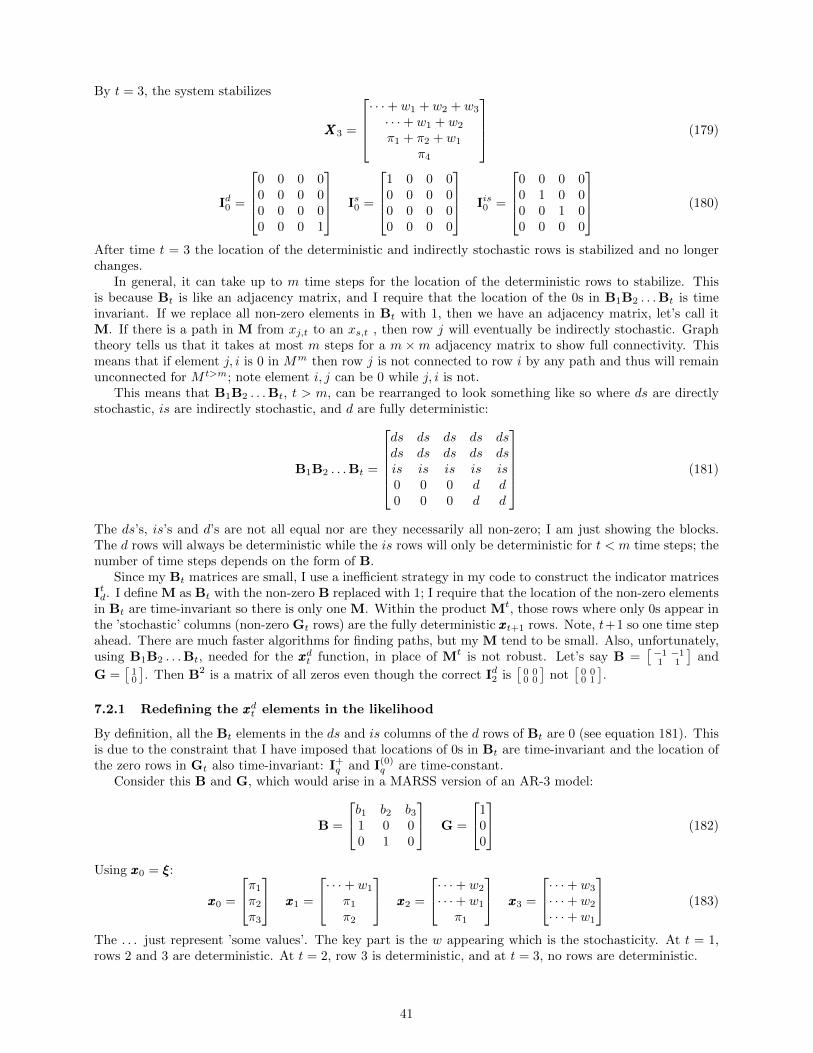
By t = 3, the system stabilizes

XXX3 =

· · ·+ w1 + w2 + w3

· · ·+ w1 + w2

π1 + π2 + w1

π4

(179)

Id0 =

0 0 0 00 0 0 00 0 0 00 0 0 1

Is0 =

1 0 0 00 0 0 00 0 0 00 0 0 0

Iis0 =

0 0 0 00 1 0 00 0 1 00 0 0 0

(180)

After time t = 3 the location of the deterministic and indirectly stochastic rows is stabilized and no longerchanges.

In general, it can take up to m time steps for the location of the deterministic rows to stabilize. Thisis because Bt is like an adjacency matrix, and I require that the location of the 0s in B1B2 . . .Bt is timeinvariant. If we replace all non-zero elements in Bt with 1, then we have an adjacency matrix, let’s call itM. If there is a path in M from xj,t to an xs,t , then row j will eventually be indirectly stochastic. Graphtheory tells us that it takes at most m steps for a m ×m adjacency matrix to show full connectivity. Thismeans that if element j, i is 0 in Mm then row j is not connected to row i by any path and thus will remainunconnected for M t>m; note element i, j can be 0 while j, i is not.

This means that B1B2 . . .Bt, t > m, can be rearranged to look something like so where ds are directlystochastic, is are indirectly stochastic, and d are fully deterministic:

B1B2 . . .Bt =

ds ds ds ds dsds ds ds ds dsis is is is is0 0 0 d d0 0 0 d d

(181)

The ds’s, is’s and d’s are not all equal nor are they necessarily all non-zero; I am just showing the blocks.The d rows will always be deterministic while the is rows will only be deterministic for t < m time steps; thenumber of time steps depends on the form of B.

Since my Bt matrices are small, I use a inefficient strategy in my code to construct the indicator matricesItd. I define M as Bt with the non-zero B replaced with 1; I require that the location of the non-zero elementsin Bt are time-invariant so there is only one M. Within the product Mt, those rows where only 0s appear inthe ’stochastic’ columns (non-zero Gt rows) are the fully deterministic xxxt+1 rows. Note, t+1 so one time stepahead. There are much faster algorithms for finding paths, but my M tend to be small. Also, unfortunately,using B1B2 . . .Bt, needed for the xxxdt function, in place of Mt is not robust. Let’s say B =

[−1 −11 1

]and

G =[

10

]. Then B2 is a matrix of all zeros even though the correct Id2 is

[0 00 0

]not

[0 00 1

].

7.2.1 Redefining the xxxdt elements in the likelihood

By definition, all the Bt elements in the ds and is columns of the d rows of Bt are 0 (see equation 181). Thisis due to the constraint that I have imposed that locations of 0s in Bt are time-invariant and the location ofthe zero rows in Gt also time-invariant: I+

q and I(0)q are time-constant.

Consider this B and G, which would arise in a MARSS version of an AR-3 model:

B =

b1 b2 b31 0 00 1 0

G =

100

(182)

Using xxx0 = ξ:

xxx0 =

π1

π2

π3

xxx1 =

· · ·+ w1

π1

π2

xxx2 =

· · ·+ w2

· · ·+ w1

π1

xxx3 =

· · ·+ w3

· · ·+ w2

· · ·+ w1

(183)

The . . . just represent ’some values’. The key part is the w appearing which is the stochasticity. At t = 1,rows 2 and 3 are deterministic. At t = 2, row 3 is deterministic, and at t = 3, no rows are deterministic.

41

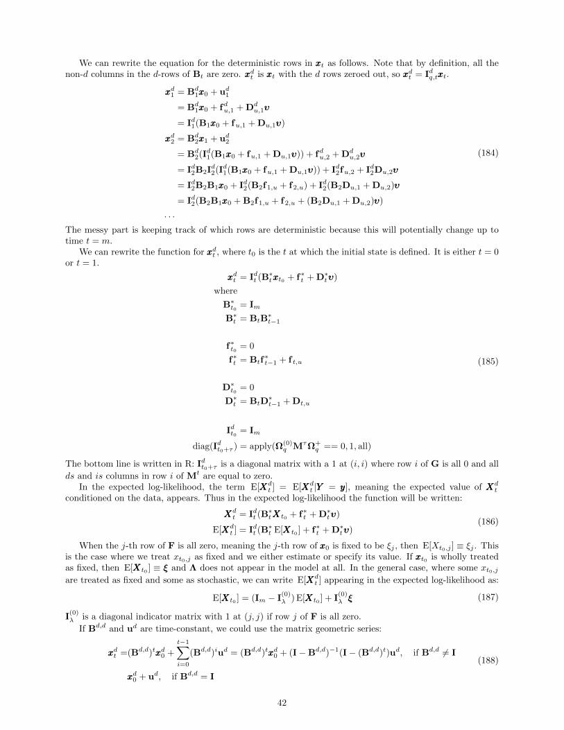
We can rewrite the equation for the deterministic rows in xxxt as follows. Note that by definition, all thenon-d columns in the d-rows of Bt are zero. xxxdt is xxxt with the d rows zeroed out, so xxxdt = Idq,txxxt.

xxxd1 = Bd1xxx0 + ud1

= Bd1xxx0 + fdu,1 + Dd

u,1υυυ

= Id1(B1xxx0 + fu,1 + Du,1υυυ)

xxxd2 = Bd2xxx1 + ud2

= Bd2(Id1(B1xxx0 + fu,1 + Du,1υυυ)) + fdu,2 + Dd

u,2υυυ

= Id2B2Id2(Id1(B1xxx0 + fu,1 + Du,1υυυ)) + Id2fu,2 + Id2Du,2υυυ

= Id2B2B1xxx0 + Id2(B2f1,u + f2,u) + Id2(B2Du,1 + Du,2)υυυ

= Id2(B2B1xxx0 + B2f1,u + f2,u + (B2Du,1 + Du,2)υυυ)

. . .

(184)

The messy part is keeping track of which rows are deterministic because this will potentially change up totime t = m.

We can rewrite the function for xxxdt , where t0 is the t at which the initial state is defined. It is either t = 0or t = 1.

xxxdt = Idt (B∗txxxt0 + f∗t + D∗tυυυ)

where

B∗t0 = Im

B∗t = BtB∗t−1

f∗t0 = 0

f∗t = Btf∗t−1 + f t,u

D∗t0 = 0

D∗t = BtD∗t−1 + Dt,u

Idt0 = Im

diag(Idt0+τ ) = apply(Ω(0)q MτΩ+

q == 0, 1, all)

(185)

The bottom line is written in R: Idt0+τ is a diagonal matrix with a 1 at (i, i) where row i of G is all 0 and all

ds and is columns in row i of Mt are equal to zero.In the expected log-likelihood, the term E[XXXd

t ] = E[XXXdt |YYY = yyy], meaning the expected value of XXXd

t

conditioned on the data, appears. Thus in the expected log-likelihood the function will be written:

XXXdt = Idt (B

∗tXXXt0 + f∗t + D∗tυυυ)

E[XXXdt ] = Idt (B

∗t E[XXXt0 ] + f∗t + D∗tυυυ)

(186)

When the j-th row of F is all zero, meaning the j-th row of xxx0 is fixed to be ξj , then E[Xt0,j ] ≡ ξj . Thisis the case where we treat xt0,j as fixed and we either estimate or specify its value. If xxxt0 is wholly treatedas fixed, then E[XXXt0 ] ≡ ξ and Λ does not appear in the model at all. In the general case, where some xt0,jare treated as fixed and some as stochastic, we can write E[XXXd

t ] appearing in the expected log-likelihood as:

E[XXXt0 ] = (Im − I(0)λ ) E[XXXt0 ] + I

(0)λ ξ (187)

I(0)λ is a diagonal indicator matrix with 1 at (j, j) if row j of F is all zero.

If Bd,d and ud are time-constant, we could use the matrix geometric series:

xxxdt =(Bd,d)txxxd0 +

t−1∑i=0

(Bd,d)iud = (Bd,d)txxxd0 + (I−Bd,d)−1(I− (Bd,d)t)ud, if Bd,d 6= I

xxxd0 + ud, if Bd,d = I

(188)

42

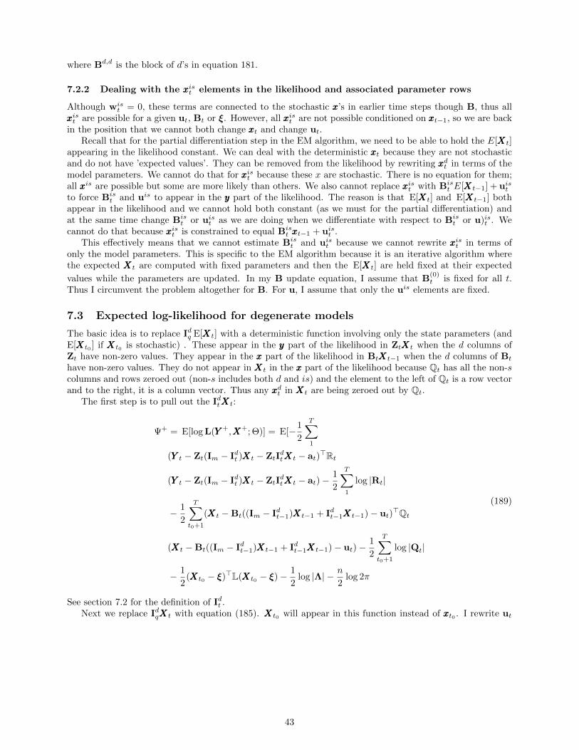
where Bd,d is the block of d’s in equation 181.

7.2.2 Dealing with the xxxist elements in the likelihood and associated parameter rows

Although wist = 0, these terms are connected to the stochastic xxx’s in earlier time steps though B, thus all

xxxist are possible for a given ut, Bt or ξ. However, all xxxist are not possible conditioned on xxxt−1, so we are backin the position that we cannot both change xxxt and change ut.

Recall that for the partial differentiation step in the EM algorithm, we need to be able to hold the E[XXXt]appearing in the likelihood constant. We can deal with the deterministic xxxt because they are not stochasticand do not have ’expected values’. They can be removed from the likelihood by rewriting xxxdt in terms of themodel parameters. We cannot do that for xxxist because these x are stochastic. There is no equation for them;all xxxis are possible but some are more likely than others. We also cannot replace xxxist with Bis

t E[XXXt−1] + uistto force Bis

t and uis to appear in the yyy part of the likelihood. The reason is that E[XXXt] and E[XXXt−1] bothappear in the likelihood and we cannot hold both constant (as we must for the partial differentiation) andat the same time change Bis

t or uist as we are doing when we differentiate with respect to Bist or u)ist . We

cannot do that because xxxist is constrained to equal Bist xxxt−1 + uist .

This effectively means that we cannot estimate Bist and uist because we cannot rewrite xxxist in terms of

only the model parameters. This is specific to the EM algorithm because it is an iterative algorithm wherethe expected XXXt are computed with fixed parameters and then the E[XXXt] are held fixed at their expected

values while the parameters are updated. In my B update equation, I assume that B(0)t is fixed for all t.

Thus I circumvent the problem altogether for B. For u, I assume that only the uis elements are fixed.

7.3 Expected log-likelihood for degenerate models

The basic idea is to replace Idq E[XXXt] with a deterministic function involving only the state parameters (andE[XXXt0 ] if XXXt0 is stochastic) . These appear in the yyy part of the likelihood in ZtXXXt when the d columns ofZt have non-zero values. They appear in the xxx part of the likelihood in BtXXXt−1 when the d columns of Bt

have non-zero values. They do not appear in XXXt in the xxx part of the likelihood because Qt has all the non-scolumns and rows zeroed out (non-s includes both d and is) and the element to the left of Qt is a row vectorand to the right, it is a column vector. Thus any xxxdt in XXXt are being zeroed out by Qt.

The first step is to pull out the IdtXXXt:

Ψ+ = E[log L(YYY +,XXX+; Θ)] = E[−1

2

T∑1

(YYY t − Zt(Im − Idt )XXXt − ZtIdtXXXt − at)

>Rt

(YYY t − Zt(Im − Idt )XXXt − ZtIdtXXXt − at)−

1

2

T∑1

log |Rt|

− 1

2

T∑t0+1

(XXXt −Bt((Im − Idt−1)XXXt−1 + Idt−1XXXt−1)− ut)>Qt

(XXXt −Bt((Im − Idt−1)XXXt−1 + Idt−1XXXt−1)− ut)−1

2

T∑t0+1

log |Qt|

− 1

2(XXXt0 − ξ)>L(XXXt0 − ξ)− 1

2log |Λ| − n

2log 2π

(189)

See section 7.2 for the definition of Idt .Next we replace IdqXXXt with equation (185). XXXt0 will appear in this function instead of xxxt0 . I rewrite ut

43

as fu,t + Du,tυυυ. This gives us the expected log-likelihood:

Ψ+ = E[log L(YYY +,XXX+; Θ)] = E[−1

2

T∑1

(YYY t − Zt(Im − Idt )XXXt − ZtIdt (B

∗tXXXt0 + f∗t + D∗tυυυ)− at)

>Rt

(YYY t − Zt(Im − Idt )XXXt − ZtIdt (B

∗tXXXt0 + f∗t + D∗tυυυ)− at)−

1

2

T∑1

log |Rt|

− 1

2

T∑t0+1

(XXXt −Bt((Im − Idt−1)XXXt−1 + Idt−1(B∗t−1XXXt0 + f∗t−1 + D∗t−1υυυ))− fu,t −Du,tυυυ)>Qt

(XXXt −Bt((Im − Idt−1)XXXt−1 + Idt−1(B∗t−1XXXt0 + f∗t−1 + D∗t−1 + υυυ))− fu,t −Du,tυυυ)

− 1

2

T∑t0

log |Qt| −1

2(XXXt0 − ξ)>L(XXXt0 − ξ)− 1

2log |Λ| − n

2log 2π

(190)

where B∗, f∗ and D∗ are defined in equation (185). Rt = Ξ>t R−1t Ξt and Qt = Φ>t Q−1

t Φt, L = Π>Λ−1Π.When xxxt0 is treated as fixed, L = 0 and the last line will drop out altogether, however in general some rowsof xxxt0 could be fixed and others stochastic.

We can see directly in equation (190) where υυυ appears in the expected log-likelihood. Where p appearsis less obvious because it depends on F, which specifies which rows of xxxt0 are fixed. From equation (187),

E[XXXt0 ] = (Im − I(0)l ) E[XXXt0 ] + I

(0)l ξ

and ξ = fξ +Dξp. Thus where p appears in the expected log-likelihood depends on the location of zero rows

in F (and thus the zero rows in the indicator matrix I(0)l ). Recall that E[XXXt0 ] appearing in the expected

log-likelihood function is conditioned on the data so E[XXXt0 ] in Ψ is not equal to ξ if xxxt0 is stochastic.The case where xxxt0 is stochastic is a little odd because conditioned on XXXt0 = xxxt0 , xxxdt is deterministic even

though XXX0 is a random variable in the model. Thus in the model, xxxdt is a random variable through XXXt0 . Butwhen we do the partial differentiation step for the EM algorithm, we hold XXX at its expected value thus weare holding XXXt0 at a specific value. We cannot do that and change u at the same time because once we fixXXXt0 the xxxdt are deterministic functions of u.

7.4 Logical constraints to ensure a consistent system of equations

We need to ensure that the model remains internally consistent when R or Q goes to zero and that we donot have an over- or under-constrained system.

As an example of a solvable versus unsolvable model, consider the following.

HtRt =

0 01 00 10 0

[a 00 b

]=

0 0 0 00 a 0 00 0 b 00 0 0 0

, (191)

then following are bad versus ok Z matrices.

Zbad =

c d 0

z(2, 1) z(2, 2) z(2, 3)z(3, 1) z(3, 1) z(3, 1)c d 0

, Zok =

c 0 0

z(2, 1) z(2, 2) z(2, 3)z(3, 1) z(3, 1) z(3, 1)c d 6= 0 0

(192)

Because yt(1) and yt(4) have zero observation variance, the first Z reduces to this for xt(1) and xt(2):[yt(1)yt(4)

]=

[cxt(1) + dxt(2)cxt(1) + dxt(2)

](193)

and since yt(1) 6= yt(4), potentially, that is not solvable. The second Z reduces to[yt(1)yt(4)

]=

[cxt(1)

cxt(1) + dxt(4)

](194)

44

and that is solvable for any yt(1) and yt(4) combination. Notice that in the latter case, xt(1) and xt(2) arefully specified by yt(1) and yt(4).

7.4.1 Constraint 1: Z does not lead to an over-determined observation process

We need to ensure that a xxxt exists for all yyy(0)t such that:

E[yyy(0)t ] = Z(0) E[xxxt] + a(0).

If Z(0) is invertible, such a xxxt certainly exists. But we do not require that only one xxxt exists, simply that atleast one exists. Thus the system can be under-constrained but not over-constrained. One way to test for thisis to use the singular value decomposition (SVD) of Z(0). If the number of singular values of Z(0) is less than

the number of columns in Z, which is the number of xxx rows, then Z(0) specifies an over-constrained system(y = Zx17) Using the R language, you would test if the length of svd(Z)$d is less than than dim(Z)[2]. If

Z(0) specifies and under-determined system, some of the singular values would be equal to 0 (within machine

tolerance). It is possible that Z(0) could specify both an over- and under-determined system at the same

time. That is, the number of singular values could be less than the number of columns in Z(0) and some ofthe singular values could be 0.

Doesn’t a Z with more rows than columns automatically specify a over-determined system? No. Consid-ered this Z 1 0

0 10 0

(195)

This Z is fine, although obviously the last row of yyy will not hold any information about the xxx. But it couldhave information about R and a, which might be shared with the other yyy, so we don’t want to prevent theuser from specifying a Z like this.

7.4.2 Constraint 2: the state processes are not over-constrained.

We also need to be concerned with the state process being over-constrained when both Q = 0 and R = 0because we can have a situation where the constraint imposed by the observation process is at odds with theconstraint imposed by the state process. Here is an example:

yyyt =

[1 00 1

] [x1

x2

]t[

x1

x2

]t

=

[1 00 0

] [x1

x2

]t−1

+

[w1

0

]t−1

(196)

In this case, some of the x’s are deterministic, Q = 0 and not linked through B to a stochastic x, andthe corresponding y are also deterministic. These cases will show up as errors in the Kalman filter/smootherbecause in the Kalman gain equation (equation 142e), the term ZtV

t−1t Z>t will appear when R = 0. We

need to make sure that 0 rows in Bt, Zt and Qt do not line up in such a way that 0 rows/cols do not appearin ZtV

t−1t Z>t at the same place as 0 rows/cols in R. In MARSS, this is checked by doing a pre-run of the

Kalman smoother to see if it throws an error in the Kalman gain step.

8 EM algorithm modifications for degenerate models

The R, Q, Z, and a update equations are largely unchanged. The real difficulties arise for the u and ξupdate equations when u(0) or ξ(0) are estimated. For B, I do not have a degenerate update equation, so Ineed to assume that B(0) elements are fixed (not estimated).

17This is the classic problem of solving the system of linear equations, which is standardly written Ax = b.

45

8.1 R and Q update equations

The constrained update equations for Q and R work fine because their update equations do not involve anyinverses of non-invertible matrices. However if HtRtH

>t is non-diagonal and there are missing values, then

the R update equation involves yt. That will involve the inverse of HtR11H>t (section 6.2), which might

have zeros on the diagonal. In that case, use the ∇t modification that deals with such zeros (equation 149).

8.2 Z and a update equations

We need to deal with Z and a elements that appear in rows where the diagonal of R = 0. These values willnot appear in the likelihood function unless they also happen to also appear on the rows where the diagonalof R is not 0 (because they are constrained to be equal for example). However, in this case the Z(0) and a(0)

are logically constrained by the equation

yyy(0)t = Z

(0)t E[xxxt] + a

(0)t .

Notice there is no wt since R = 0 for these rows. The E[xxxt] is ML estimate of xxxt computed in the Kalmansmoother from the parameter values at iteration i of the EM algorithm, so there is no information in thisequation for Z and a at iteration i + 1. The nature of the smoother is that it will find the xxxt that is mostconsistent with the data. For example if our y = Zx+ a equation looks like so[

02

]=

[11

]x, (197)

there is no x that will solve this. However x = 1 is the closest (lowest squared error) and so this is theinformation in the data about x. The Kalman filter will use this and the relative value of Q and R to comeup with the estimated x. In this case, R = 0, so the information in the data will completely determine x andthe smoother would return x = 1 regardless of the process equation.

The a and Z update equations require that∑Tt=1 D>t,aRtDt,a and

∑Tt=1 D>t,zRtDt,z are invertible. If Z

(0)t

and a(0)t are fixed, this will be satisfied, however the restriction is a little less restrictive than that since it

is possible that Rt does not have zeros on the diagonal in the same places so that the sum over t could beinvertible while the individual values at t are not. The section on the summary of constraints has the testfor this constraint.

The update equations also involve yt, and the modified algorithm for yt when Ht has all zero rows willbe needed. Other than that, the constrained update equations work (sections 5.2 and 5.7).

8.3 u update equation

Here I discuss the update for u, or more specifically υυυ which appears in u, when Gt or Ht have zero rows. Irequire that uist is not estimated. All the uist are fixed values. The udt may be estimated or more specificallythere may be υυυ in udt that are estimated; udt = fdu,t + Dd

u,tυυυ.For the constrained u update equation with deterministic xxx’s takes the following form. It is similar to

the unconstrained update equation except that that a part from the yyy part of the likelihood now appears:

υυυj+1 =

( T∑t=1

(∆>t,2Rt∆t,2 + ∆>t,4Qt∆t,4)

)−1

×( T∑t=1

(∆>t,2Rt∆t,1 + ∆>t,4Qt∆t,3

))(198)

Conceptually, I think the approach described here is the similar to the approach presented in section 4.2.5of (Harvey, 1989), but it is more general because it deals with the case where some u elements are shared(linear functions of some set of shared values), possibly across deterministic and stochastic elements. Also, Ipresent it here within the context of the EM algorithm, so solving for the maximum-likelihood u appears inthe context of maximizing Ψ+ with respect to u for the update equation at iteration j + 1.

8.3.1 u(0) is not estimated

When u(0) is not estimated (since it is at some user defined value via Du and fu), the part we are estimating,u+, only appears in the xxx part of the likelihood. The update equation for u remains equation (97).

46

8.3.2 ud is estimated

The derivation of the update equation proceeds as usual. We need to take the partial derivative of Ψ+

(equation 190) holding everything constant except υυυ, elements of which might appear in both udt and ust (butnot uist since I require that uist has no estimated elements).

The expected log-likelihood takes the following form, where t0 is the time where the initial state is defined(t = 0 or t = 1):

Ψ+ = −1

2

T∑1

(∆t,1 −∆t,2υυυ)>Rt(∆t,1 −∆t,2υυυ)− 1

2

T∑1

log |Rt|

−1

2

T∑t0+1

(∆t,3 −∆t,4υυυ)>Qt(∆t,3 −∆t,4υυυ)− 1

2

T∑t0+1

log |Qt|

−1

2(XXXt0 − ξ)>L(XXXt0 − ξ)− 1

2log |Λ| − n

2log 2π

(199)

L = F>Λ−1F. If xxxt0 is treated as fixed, F is all zero and the line with L drops out. If some but not all xxxt0are treated as fixed, then only the stochastic rows appear in the last line. In any case, the last line does notcontain υυυ, thus when we do the partial differentiation with respect to υυυ, this line drops out.

The ∆ terms are defined as:

∆t,1 = yt − Zt(Im − Idt )xt − ZtIdt (B

∗t E[XXXt0 ] + f∗t )− at

∆t,2 = ZtIdtD∗t

∆t0,3 = 0m×1

∆t,3 = xt −Bt(Im − Idt−1)xt−1 −BtIdt−1(B∗t−1 E[XXXt0 ] + f∗t−1)− f t,u

∆t0,4 = 0m×mD1,u

∆t,4 = Dt,u + BtIdt−1D

∗t−1

E[XXXt0 ] = ((Im − I(0)λ )xxxt0 + I

(0)λ ξ)

(200)

Idt , B∗t , f t∗, and D∗t are defined in equation (185). The values of these at t0 is special so that the math worksout. The expectation ( E) has been subsumed into the ∆s since ∆2 and ∆4 do not involve XXX or YYY , so termslike XXX>XXX never appear.

Take the derivative of this with respect to υυυ and arrive at:

υυυj+1 =( T∑t=1

∆>t,4Qt∆t,4 +

T∑t=1

∆>t,2Rt∆t,2

)−1 ×( T∑t=1

∆>1,4Qt∆1,3 +

T∑t=1

∆>t,2Rt∆t,1)

)(201)

8.4 ξ update equation

8.4.1 ξ is stochastic

This means that none of the rows of F (in Fλ) are zero, so I(0)λ is all zero and the update equation reduces

to a constrained version of the classic ξ update equation:

pj+1 =(D>ξ Λ−1Dξ

)−1D>ξ Λ−1( E[XXXt0 ]− fξ) (202)

8.4.2 ξ(0) is not estimated

When ξ(0) is not estimated (because you fixed it as some value), we do not need to take the partial derivative

with respect to ξ(0) since we will not be estimating it. Thus the update equation is unchanged from theconstrained update equation.

47

8.4.3 ξ(0) is estimated

Using the same approach as for u update equation, we take the derivative of (190) with respect to p whereξ = fξ + Dξp. Ψ+ will take the following form:

Ψ+ =

− 1

2

T∑t=1

(∆t,5 −∆t,6p)>Rt(∆t,5 −∆t,6p)− 1

2

T∑1

log |Rt|

− 1

2

T∑t=1

(∆t,7 −∆t,8p)>Qt(∆t,7 −∆t,8p)− 1

2

T∑1

log |Qt|

− 1

2( E[XXXt0 ]− fξ −Dξp)>L( E[XXXt0 ]− fξ −Dξp)− 1

2log |Λ|

− n

2log 2π

(203)

The ∆’s are defined as follows using E[XXXt0 ] = (Im − I(0)l )xxxt0 + I

(0)l ξ where it appears in Idt E[XXXt].

∆t,5 = yt − Zt(Im − Idt )xt − ZtIdt (B

∗t ((Im − I

(0)λ )xxxt0 + I

(0)λ fξ) + u∗t )− at

∆t,6 = ZtIdtB∗t I

(0)λ Dξ

∆t0,7 = 0m×1

∆t,7 = xt −Bt(Im − Idt−1)xt−1 −BtIdt−1(B∗t−1((Im − I

(0)l )xxxt0 + I

(0)λ fξ) + u∗t−1)− ut

∆t0,8 = 0m×mDξ

∆t,8 = BtIdt−1B

∗t−1I

(0)λ Dξ

u∗t = f∗t + D∗tυυυ

(204)

The expectation can be pulled inside the ∆s since the ∆s in front of p do not involve XXX or YYY .Take the derivative of this with respect to p and arrive at:

pj+1 =( T∑t=1

∆>t,8Qt∆t,8 +

T∑t=1

∆>t,6Rt∆t,6 + D>ξ LDξ

)−1×

( T∑t=1

∆>1,8Qt∆1,7 +

T∑t=1

∆>t,6Rt∆t,5 + D>ξ L( E[XXXt0 ]− fξ)

) (205)

8.4.4 When Ht has 0 rows in addition to Gt

When Ht has all zero rows, some of the p or υυυ may constrained by the model, but these constraints do notappear in Ψ+ since Rt zeros out those constraints. For example, if Ht is all zeros and xxx1 ≡ ξ, then ξ isconstrained to equal Z−1(y1 − a1).

The model needs to be internally consistent and we need to be able to estimate all the p and the υυυ. Ratherthan try to estimate the correct p and υυυ to ensure internal consistency of the model with the data whensome of the Ht have 0 rows, I test by running the Kalman filter with the degenerate variance modification(in particular the modification for F with zero rows is critical) before starting the EM algorithm. Then Itest that yt − Ztxt − at is all zeros. If it is not, within machine accuracy, then there is a problem. This isreported and the algorithm stopped18

I also test that(∑T

t=1 ∆>t,8Qt∆t,8 +∑Tt=1 ∆>t,6Rt∆t,6 + D>ξ LDξ

)is invertible to ensure that all the p can

be solved for, and I test that(∑T

t=1 ∆>t,4Qt∆t,4 +∑Tt=1 ∆>t,2Rt∆t,2

)is invertible so that all the υυυ can be

solved for. If errors are present, they should be apparent in iteration 1, are reported and the EM algorithmstopped.

18In some cases, it is easy to determine the correct ξ. For example, when Ht is all zero rows, t0 = 1 and there is no missingdata at time t = 1, ξ = Z∗(yyy1 − a1), where Z∗ is the pseudoinverse. One would want to use the SVD pseudoinverse calculationin case Z leads to an under-constrained system (some of the singular values of Z are 0).

48

8.5 B(0) update equation for degenerate models

I do not have an update equation for B(0) and for now, I side-step this problem by requiring that any B(0)

terms are fixed.

9 Kalman filter and smoother modifications for degenerate models

9.1 Modifications due to degenerate R and Q

[1/1/2012 note. These modifications mainly have to do with inverses that appear in the Shumway andStoffer’s presentation of the Kalman filter. Later I want to switch to Koopman’s smoother algorithm whichavoids these inverses altogether.]

In principle, when either GtQt or HtRt has zero rows, the standard Kalman filter/smoother equationswould still work and provide the correct state outputs and likelihood. In practice however errors will begenerated because under certain situations, one of the matrix inverses in the Kalman filter/smoother equationswill involve a matrix with a zero on the diagonal and this will lead to the computer code throwing an error.

When HtRt has zero rows, problems arise in the Kalman update part of the Kalman filter. The Kalmangain is

Kt = Vt−1t (Z∗t )

>(Z∗tVt−1t (Z∗t )

> + HtR∗tH>t )−1 (206)

Here, Z∗t is the missing values modified Zt matrix with the i-th rows zero-ed out if the i-th element of yyyt ismissing (section 6.1, equation 144). Thus if the i-th element of yyyt is missing and the i-th row of Ht is zero,the (i, i) element of (Z∗tV

t−1t (Z∗t )

>+HtR∗tH>t ) will be zero also and one cannot take its inverse. In addition,

if the initial value xxx1 is treated as fixed but unknown then V01 will be a m×m matrix of zeros. Again in this

situation (Z∗tVt−1t (Z∗t )

> + HtR∗tH>t ) will have zeros at any (i, i) elements where the i-th row of Ht is also

zero.The first case, where zeros on the diagonal arise due to missing values in the data, can be solved using

the matrix which pulls out the rows and columns corresponding to the non-missing values (Ω(1)t ). Replace(

Z∗tVt−1t (Z∗t )

> + HtR∗tH>t

)−1in equation (206) with

(Ω(1)t )>

(Ω

(1)t (Z∗tV

t−1t (Z∗t )

> + HtR∗tH>t )(Ω

(1)t )>

)−1Ω

(1)t (207)

Wrapping in Ω(1)t (Ω

(1)t )> gets rid of all the zero rows/columns in Z′tV

t−1t (Z′t)

> + HtR′tH>t , and the matrix

is reassembled with the zero rows/columns reinserted by wrapping in (Ω(1)t )>Ω

(1)t . This works because R′t is

the missing values modified R (section 1.3) and is block diagonal across the i and non-i rows/columns, andZ′t has the i-columns zero-ed out. Thus removing the i columns and rows before taking the inverse has noeffect on the product Zt(...)

−1. When V01 = 0, set K1 = 0 without computing the inverse (see equation 206

where V01 appears on the left).

There is also a numerical issue to deal with. When the i-th row of Ht is zero, some of the elements ofxxxt may be completely specified (fully known) given yyyt. Let’s call these fully known elements of xxxt, the k-thelements. In this case, the k-th row and column of Vt

t must be zero because given yt(i), xt(k) is known(is fixed) and its variance, Vt

t(k, k), is zero. Because Kt is computed using a numerical estimate of theinverse, the standard Vt

t update equation (which uses Kt) will cause these elements to be close to zero butnot precisely zero, and they may even be slightly negative on the diagonal. This will cause serious problemswhen the Kalman filter output is passed on to the EM algorithm. Thus after Vt

t is computed using thenormal Kalman update equation, we will want to explicitly zero out the k rows and columns in the filter.

When Gt has zero rows, then we might also have similar numerical errors in J in the Kalman smoother.The J equation is

Jt = Vt−1t−1B

>t (Vt−1

t )−1

where Vt−1t = BtV

t−1t−1B

>t + GtQtG

>t

(208)

If there are zeros on the diagonals of (Λ and/or Bt) and zero rows in Gt and these zeros line up, then if the

B(0)t and B

(1)T elements in Bt are blocks19, there will be zeros on the diagonal of Vt

t. Thus there will be zeros

19This means the following. Let the rows where the diagonal elements in Q equal zero be denoted i and the the rows where

49

on the diagonal of Vt−1t and it cannot be inverted. In this case, the corresponding elements of VT

t need tobe zero since what’s happening is that those elements are deterministic and thus have 0 variance.

We want to catch these zero variances in Vt−1t so that we can take the inverse. Note that this can only

happen when there are zeros on the diagonal of GtQtG>t since BtV

t−1t−1B

>t can never be negative on the

diagonal since BtB>t must be positive-definite and so is Vt−1

t−1. The basic idea is the same as above. We

replace (Vt−1t )−1 with:

(Ω+V t)>(Ω+

V t(Vt−1t )(Ω+

V t)>)−1

Ω+V t (209)

where Ω+V t is a matrix that removes all the positive Vt−1

t rows analogous to Ω(1)t .

9.2 Modifications due to fixed initial states

When the initial state of xxx is fixed, then it is a bit like Λ = 0 although actually Λ does not appear in themodel and ξ has a different interpretation.

When the initial state of xxx is treated as stochastic, then if t0 = 0, ξ is the expected value of xxx0 conditionedon no data. In the Kalman filter this means xxx0

0 = ξ and V00 = Λ; in words, the expected value of xxx0

conditioned on yyy0 is ξ and the variance of xxx00 conditioned on yyy0 is Λ. When t0 = 1, then ξ is the expected

value of xxx1 conditioned on no data. In the Kalman filter this means xxx01 = ξ and V0

1 = Λ. Thus where ξ andΛ appear in the Kalman filter equations is different depending on t0; the xxxtt and Vt

t initial condition versusthe xxxt−1

t and Vt−1t initial condition.

When some or all of the xxxt0 are fixed, denoted the I(0)λ xxxt0 , the fixed values are not a random variables.

While technically speaking, the expected value of a fixed value does not exist, we can think of it as a random

variable with a probability density function with all the weight on the fixed value. Thus I(0)λ E[xxxt0 ] = ξ

regardless of the data. The data have no information for I(0)λ xxxt0 since we fix I

(0)λ xxxt0 at I

(0)λ ξ. If t0 = 0, we

initialize the Kalman filter as usual with xxx00 = ξ and V0

0 = FΛF>, where the fixed xxxt0 rows correspond tothe zero row/columns in FΛF>. The Kalman filter will return the correct expectations even when some ofthe diagonals of HRH> or GQG> are 0—with the constraint that we have no purely deterministic elementsin the model (meaning there are no errors terms from either R or Q).

When t0 = 1, I(0)λ xxx0

1 and I(0)l xxx1

1 = ξ regardless of the data and V01 = FΛF> and V1

1 = FΛF>, where the

fixed rows of xxx1 correspond with the 0 row/columns in FΛF>. We also set I(0)λ K1, meaning the rows of xxx1

that are fixed, to all zero because K1 is the information in yyy1 regarding xxx1 and there is no information in

the data regarding the values of xxx1 that are fixed to equal I(0)λ ξ.

With V11, xxx1

1 and K1 set to their correct initial values, the normal Kalman filter equations will work fine.However it is possible for the data at t = 1 to be inconsistent with the model if the rows of yyy1 correspondingto any zero row/columns in Z1FΛF>Z>1 + H1R1H

>1 are not equal to Z1ξ + a1. Here is a trivial example,

let the model be xt = xt−1 + wt, yt = xt, x1 = 1. Then if y1 is anything except 1, the model is impossible.Technically, the likelihood of x1 conditioned on Y1 = y1 does not exist since neither x1 nor y1 are realizationsof a random variable (since they are fixed), so when the likelihood is computed using the innovations formof the likelihood, the t = 1 does not appear, at least for those yyy1 corresponding to any zero row/columnsin Z1FΛF>Z>1 + H1R1H

>1 . Thus these internal inconsistencies would neither provoke an error nor cause

Inf to be returned for the likelihood. In the MARSS package, the Kalman filter has been modified to returnLL=Inf and an error.

10 Summary of requirements for degenerate models

Below are discussed the update equations for the different parameters. Here I summarize the constraints thatare scattered throughout these subsections. These requirements are coded into the function MARSSkem-check() in the MARSS package but some tests must be repeated in the function degen.test(), which tests ifany of the R or Q diagonals can be set to zero if it appears they are going to zero. A model that is allowedwhen R and Q are non-zero, might be disallowed if R or Q diagonals were to be set to zero. degen.test()does this check.

there are non-zero diagonals be denoted j. The B(0)t elements are the Bt elements where both row and column are in i. The

B(1)t elements are the B elements where both row and column are in j. If the B

(0)t and B

(1)t elements in B are blocks, this

means all the Bt(i, j) are 0; no deterministic components interact with the stochastic components.

50

(Im ⊗ I(0)r ZtI

(0)q )Dt,b, is all zeros. If there is a all zero row in Ht and it is linked (through Z) to a

all zero row in Gt, then the corresponding Bt elements are fixed instead of estimated. CorrespondingB rows means those rows in B where there is a non-zero column in Z. We need I(0)

r ZtI(0)q Bt to only

specify fixed Bt elements, which means vec(I(0)r ZtI

(0)q BtIm) only specifies fixed values. This in turn

leads to the condition above. MARSSkemcheck()

(I1 ⊗ I(0)r ZtI

(0)q )Dt,u is all zeros; if there is a all zero row in Ht and it is linked (through Zt) to a all

zero row in Gt, then the corresponding ut elements are fixed instead of estimated. MARSSkemcheck()

(Im ⊗ I(0)r )Dt,z, where is all zeros; if y has no observation error, then the corresponding Zt rows are

fixed values. (Im ⊗ I(0)r ) is a diagonal matrix with 1s for the rows of Dt,z that correspond to elements

of Zt on the R = 0 rows. MARSSkemcheck()

(I1⊗I(0)r )Dt,a is all zeros; if y has no observation error, then the corresponding at rows are fixed values.

MARSSkemcheck()

(Im ⊗ I(0)q )Dt,b is all zeros. This means B(0) (the whole row) is fixed. While Bd could potentially be

estimated potentially, my derivation assumes it is not. MARSSkemcheck()

(I1⊗Iisq,t>m)Dt,u is all zeros. This means uis is fixed. Here is is defined as those rows that are indirectlystochastic at time m, where m is the dimension of B; it can take up to m steps for the is rows to beconnected to the s rows through B. MARSSkemcheck()

If u(0) or ξ(0) are being estimated, then the adjacency matrices defined by Bt 6= 0 are not time-varying. This means that the locations of the 0s in Bt are not changing over time. Bt however may betime-varying. MARSSkemcheck()

I(0)q and I(0)

r are time invariant (an imposed assumption). This means that the location of the 0 rows inGt and Ht (and thus in wt and vt) are not changing through time. It would be easy enough to allow

I(0)r to be time varying, but to make my derivation easier, I assume it is time constant.

Z(0)t in E[YYY

(0)t ] = Z

(0)t E[XXXt]+a

(0)t does not imply an over-determined system of equations. Because the

vt rows are zero for the (0) rows of yyy, it must be possible for this equality to hold. This means that Z(0)t

cannot specify an over-determined system although an underdetermined system is ok. MARSSkem-

check() checks by examining the singlular values of Z(0)t returned from the singlular value decomposition

(svd). The number of singlular values must not be less than m (columns of Z). If it is less than m, itmeans the equation system is over-determined. Singular values equal to 0 are ok; it means the systemis under-determined given only the observation equation, but that’s ok because we also have the stateequation will determine the under states and the Kalman smoother will presumably throw an error ifthe state process is under-determined (if that would even make sense...).

The state process cannot be over-determined via constraints imposed from the deterministic observationprocess (R = 0) and the deterministic state process (Q = 0). If this is the case the Kalman gain equation(in the Kalman filter) will throw an error. Checked in MARSS() via call to MARSSkf() before fittingcall; degen.test(), in MARSSkem() will also test via MARSSkf call if some R or Q are attempted to beset to 0. If B or Z changes during kem or optim iterations such that this constraint does not hold, thenalgorithm will exit with an error message.

The location of the 0s in B are time-invariant. The B can be time-varying but not the location of 0s.Also, I want B to be such that once a row becomes indirectly stochastic is stays that way. For example,if B =

[0 11 0

], then row 2 flips back and forth from being indirectly stochastic to deterministic.

The dimension of the identity matrices in the above constraints is given by the subscript on I except whenit is implicit.

51

11 Implementation comments

The EM algorithm is a hill-climbing algorithm and like all hill-climbing algorithms it can get stuck on localmaxima. There are a number approaches to doing a pre-search of the initial conditions space, but a brute forcerandom Monte Carol search appears to work well (Biernacki et al., 2003). It is slow, but normally sufficient.However an initial conditions search should be done before reporting final estimates for an analysis. Inour papers on the distributional properties of MARSS parameter estimates, we rarely found that an initialconditions search changed the estimates—except in cases where Z and B are estimated as unconstrained andas the fraction of missing data in the data set became large.

The EM algorithm will quickly home in on parameter estimates that are close to the maximum, but oncethe values are close, the EM algorithm can slow to a crawl. Some researchers start with an EM algorithmto get close to the maximum-likelihood parameters and then switch to a quasi-Newton method for the finalsearch. In many ecological applications, parameter estimates that differ by less than 3 decimal places are forall practical purposes the same. Thus we have not used the quasi-Newton final search.

Shumway and Stoffer (2006; chapter 6) imply in their discussion of the EM algorithm that both ξ and Λcan be estimated, though not simultaneously. Harvey (1989), in contrast, discusses that there are only twoallowable cases for the initial conditions: 1) fixed but unknown and 2) a initial condition set as a prior. Incase 1, ξ is xxx0 (or xxx1) and is then estimated as a parameter; Λ is held fixed at 0. In case 2, ξ and Λ specifythe mean and variance of XXX0 (or XXX1) respectively. Neither are estimated; instead, they are specified as partof the model.

As mentioned in the introduction, misspecification of the prior on xxx0 can have catastrophic and unde-tectable effects on your parameter estimates. For many MARSS models, you will never see this problem.However, if you are fitting models that imply a correlation structure between the hidden states (i.e. thevariance-covariance matrix of the XXX’s is not diagonal), then your prior can definitely create problems if itdoes not have the same correlation structure as that implied by your MLE model. A common default is to usea prior with a diagonal variance-covariance matrix. This can lead to serious problems if the implied variance-covariance of the XXX’s is not diagonal. A diffuse prior does not get around this since it has a correlationstructure also even if it has infinite variance.

One way you can detect that you have a problem is to start the EM algorithm at the outputs from aNewton-esque algorithm. If the EM estimates diverge and the likelihood drops, you have a problem. Hereare a few suggestions for getting around the problem:

Treat xxx0 as an estimated parameter and set V0=0. If the model is not stable going backwards in time,then treat xxx1 as the estimated parameter; this will allow the data to constrain the xxx1 estimate (sincethere is no data at t = 0, xxx0 has no data to constrain it).

Try a diffuse prior, but first read the info in the KFAS R package about diffuse priors since MARSS usesthe KFAS implementation. In particular, note that you will still be imposing an information on thecorrelation structure using a diffuse prior; whatever V0 you use is telling the algorithm what correlationstructure to use. If there is a mismatch between the correlation structure in the prior and the correlationstructure implied by the MLE model, you will not be escaping the prior problem. But sometimes youwill know your implied correlation structure. For example, you may know that the xxx’s are independentor you may be able to solve for the stationary distribution a priori if your stationary distribution is nota function of the parameters you are trying to estimate. Other times you are estimating a parameterthat determines the correlation structure (like B) and you will not know a priori what the correlationstructure is.

In some cases, the update equation for one parameter needs other parameters. Technically, the Kalmanfilter/smoother should be run between each parameter update, however following Ghahramani and Hinton(1996) the default MARSS algorithm skips this step (unless the user sets control$safe=TRUE) and eachupdated parameter is used for subsequent update equations. If you see warnings that the log-likelihooddrops, then try setting control$safe=TRUE. This will increase computation time greatly.

12 MARSS R package

R code for the Kalman filter, Kalman smoother, and EM algorithm is provided as a separate R package,MARSS, available on CRAN (http://cran.r-project.org/web/packages/MARSS). MARSS was developed by

52

Elizabeth Holmes, Eric Ward and Kellie Wills and provides maximum-likelihood estimation and model-selection for both unconstrained and constrained MARSS models. The package contains a detailed userguide which shows various applications. In addition to model fitting via the EM algorithm, the packageprovides algorithms for bootstrapping, confidence intervals, auxiliary residuals, and model selection criteria.

References

Biernacki, C., Celeux, G., and Govaert, G. (2003). Choosing starting values for the EM algorithm forgetting the highest likelihood in multivariate gaussian mixture models. Computational Statistics and DataAnalysis, 41(3-4):561–575.

Borman, S. (2009). The expectation maximization algorithm - a short tutorial.

Ghahramani, Z. and Hinton, G. E. (1996). Parameter estimation for linear dynamical systems. TechnicalReport CRG-TR-96-2, University of Totronto, Dept. of Computer Science.

Harvey, A. C. (1989). Forecasting, structural time series models and the Kalman filter. Cambridge UniversityPress, Cambridge, UK.

Henderson, H. V. and Searle, S. R. (1979). Vec and vech operators for matrices, with some uses in jacobiansand multivariate statistics. The Canadian Journal of Statistics, 7(1):65–81.

Johnson, R. A. and Wichern, D. W. (2007). Applied multivariate statistical analysis. Prentice Hall, UpperSaddle River, NJ.

Koopman, S. and Ooms, M. (2011). Forecasting economic time series using unobserved components timeseries models, pages 129–162. Oxford University Press, Oxford.

Koopman, S. J. (1993). Distrubance smoother for state space models. Biometrika, 80(1):117–126.

McLachlan, G. J. and Krishnan, T. (2008). The EM algorithm and extensions. John Wiley and Sons, Inc.,Hoboken, NJ, 2nd edition.

Roweis, S. and Ghahramani, Z. (1999). A unifying review of linear gaussian models. Neural Computation,11:305–345.

Shumway, R. and Stoffer, D. (2006). Time series analysis and its applications. Springer-Science+BusinessMedia, LLC, New York, New York, 2nd edition.

Shumway, R. H. and Stoffer, D. S. (1982). An approach to time series smoothing and forecasting using theEM algorithm. Journal of Time Series Analysis, 3(4):253–264.

Wu, L. S.-Y., Pai, J. S., and Hosking, J. R. M. (1996). An algorithm for estimating parameters of state-spacemodels. Statistics and Probability Letters, 28:99–106.

Zuur, A. F., Fryer, R. J., Jolliffe, I. T., Dekker, R., and Beukema, J. J. (2003). Estimating common trendsin multivariate time series using dynamic factor analysis. Environmetrics, 14(7):665–685.

53

Derivation of an EM algorithm for constrained and …€¦ · · 2018-04-14Derivation of an EM...

Documents

Transcript of Derivation of an EM algorithm for constrained and …€¦ · · 2018-04-14Derivation of an EM...