Keskustelualoitteita #43 Joensuun yliopisto, Taloustieteet

Deregulation of Finnish Electricity Markets:

Market Structure, Regional and Distribution Network Sharing Effects on District Heating Prices in Finland 1996-2002

Mikael Linden Päivi Peltola-Ojala

ISBN 978-952-458-919-2 ISSN 1795-7885

no 43

Deregulation of Finnish Electricity Markets:

Market Structure, Regional and Distribution Network Sharing

Effects on District Heating Prices in Finland 1996-2002 1)

Mikael Linden* & Päivi Peltola-Ojala Department of Business and Economics University of Joensuu, Finland MARCH 2007 Abstract We propose an empirical econometric panel data model to test deregulation and regional market structure effects on district heating prices in Finland 1996-2002. The data consists of 76 district heating firms in Finland. Special emphasis is put on the modeling of policy induced competition started in year 1999, regional based fuel selection, market structure, and distribution network sharing effects on district heating prices. The results imply that the local structures of energy production and selling have an important role on market prices and the price lowering effects of energy market deregulation have been permanent. __________________________ 1) Paper presented at the 30th IAEE-07 World Congress in Wellington, 18th-21st of February 2007. *) Address of corresponding author: Mikael Linden, Department Business and Economics, BOX 111, Yliopistokatu 2 (Aurora II), FIN-80101, E-mail: mika.linden@joensuu.fi

I. Introduction After decades of state ownership and heavy government regulation heat and power sectors

worldwide are being deregulated. Finland is not exception in this global wave. However in

Finland, a sparse inhabited country, the implementation of policy change is demanding task.

The national energy markets are still typically dominated by a small number of producers.

Even large geographic areas are dominated by one firm. When analysis is focused on the

district heating markets, the restructuring can even be impossible. The reason for this meager

result hinges on the general and specific features of Finnish electricity and district heating

markets.

Generally market power is a prominent issue in the current debate about electricity and heat

industry restructuring. Increasing the number of sellers in a market does not necessarily

reduce market power as the standard theory suggest. Location advantages, contracts and

vertical integration allow some firms to maintain profits and prices near to monopoly levels

even the seller concentration is at levels generally considered competitive. In electricity

markets independent national transmission system with enough capacity allows for local

competition from companies outside. In contrary to this presence of transmission bottlenecks

and peak load periods may induce temporal local market power even for a firm with small

market share. However in district heating markets the heat transmission network is highly

localized and no interconnections are technically or economically feasible over larger areas.

Only in some big towns and in highly urbanized regions many producers may share the same

network. Notice also that in some cases energy input substitution is possible for the small

house owners. However the change of the form of energy input for warming in the highly

horizontally and vertically integrated markets is not necessarily a competitive increasing act.

Also the restructuring gain of firms to producer, distribution and retail seller markets is low if

the number of firms is already low in the local markets.

In following we analyze in details the Finnish district heating markets in years 1996-2002

with a firm level data. Our theoretical background is in the industrial organization literature

(IO) that stresses the importance of firm’s market share on its pricing policy. We build an

empirical econometric model that focuses on three specific pricing effects in connection to

the firm’s market share in energy production and retail markets: the effects competition

1

induced policy reform, the effects of sharing distribution network, and the effects of regional

based fuel dependency.

The household electricity markets in Finland were opened to competition in the 1st of

November 1998. Regulation was only extended to limit the unreasonable pricing and to

separate the different business units (production, distribution and sales). However the district

heating industry is still simply regulated by the general Competition Laws. The policy

induced competition in the electricity industry in late 1998 is expected to affect the district

heating industry since both industries compete in the same heating goods markets. The

industry is also constantly monitored and faces a threat of intensive regulation by the state

authorities. The price effects of induced competition are modelled in regression model

framework with different trend break and dummy variable specifications.

Geographically household heating product markets are limited to the area which is covered

by the local district heating (warm water) pipe network. In Finland, most district heat

companies are isolated from each other. Typically they have a local monopoly both in heat

distribution and production. Many companies also produce both heat and electricity (CHP).

A distribution company may also have no own production at all. These companies have the

monopoly in heat distribution and they usually buy the district heat from separate producer.

Still there exist some regions where the district heating network is shared by different

production or distribution companies. All these market structures are expected to have effects

on competition and prices in the wholesale and retail heat markets. These prices effects are

analyzed by adding to estimated models firm’s market share (both in production and heat sale

markets) in local markets. An interaction model alternative is estimated also where network

sharing dummy variable interacts with other model variables. The estimates test the

extension of network sharing firms’ different response to control variables. The network

effects are also connected to regional analysis.

The regional pricing structure is also affected by the fuel type used by the local district

heating company. In the Northern and Eastern Finland where winters are colder than in the

other parts of Finland the heat production differs from the rest of country. The price of fuels

2

is important in regional context. Natural gas is supplied (from Russia) only to the Southern

Finland, peat and wood are used mainly in the Eastern and Northern Finland, and coal is the

main fuel input on the coastal area (western Finland). We build a (3x2) -cross-classifying

dummy variable reflecting the regional location and network sharing in these regions. This

solution enables us to test at same time the network and regional specific price effects.

The structure of paper is as follows. Section 2 gives shot review non-competitive aspects of

energy pricing related to economy theory. Section 3 gives a closer look at Finnish district

heating markets. Section 4 introduces our econometric methods, specifications with relevant

pricing variables, and hypotheses tests. Section 5 focuses on the obtained results, and Section

6 concludes the paper. Appendices I-II provide a more detailed picture of econometric model

specification used in the study. Appendices III-IV report the analyzed data and some

supplementary regression results.

2. Economic theory Earlier energy and heat production and distribution were considered to be public utilities that

provided their services equally to all members of society, both to industry and to private

consumers. The target was delivery security, smoothed prices and tariffs, and equal access.

This “public goods” framework was understandable in political climate of era 1950-1970.

Also the huge grounding costs of energy plants and distribution networks supported the

public solution to the development of energy sector. Since 1980’s the political climate has

changed toward private market solutions emphasizing the importance of market based

pricing rules, competition and efficiency in production and distribution. Privatization and

deregulation were seen as policy alternatives for these targets. The case of natural

monopolies with price regulation and subsidies were buried as the huge grounding costs were

paid after decades of operation. The case of small and declining fixed costs was the new

paradigm leading to the marginal cost price rule supported by competitive markets. However

the privatization is not a necessary - not even sufficient condition - for market based solution

to energy pricing. The real question is the market structure, i.e. number of operating firms in

the markets, not the ownership form of the firms. Monopoly or what ever other non-

competitive price conduct can be formulated without reference to the ownership of firms. In

3

theory all of many companies in the competitive market can be public owned or in the other

end we have only one private owned monopoly. However in reality, especially in energy

markets with their background in public (natural) monopolies, things are more complicated

with localized markets, weak product substitution of energy products, and with horizontal

and vertical integration of markets.

The case of pure monopoly is well-formulated in economic theory. The monopoly sets its

product price above the competitive efficient market price and naturally sells less. The

monopoly facing the whole local market demand curve can conduct price discrimination

leading to increased output. This social gain is however small compared to the total

monopoly loss due the monopoly pricing. When the number of firms in the market increases,

the number of firms matter, but also their relative market shares play a crucial role. The

oligopoly is an interesting case with dynamic rivalry. In pure theory co-operative solution

boils down to cartel solution having price conduct of multi-plant monopolist. The non co-

operative case leads us to many solutions and concepts of game theory. Typically in this

literature conditions for the equilibrium with stability are demanding and refer to few cases

found in real markets. Because of complexity of the issue there is no reason why price should

fall to the level where it equals marginal cost. The Bertrand-Nash equilibrium, where price is

decision variable in homogenous product oligopoly, is the exception. When number of

players increases the role of relative magnitude of players (i.e. market shares) is important for

market pricing. With high entry costs and with some product differentiation the dominant

firm can still behave close to monopoly (Waterson 1984, Tirole 1989).

In the context of energy markets the product differentiation is not so important issues as the

vertical integration. Typically the same company owns the production, distribution and

selling of the energy to end users. In some cases the company may also be a multi-product

company, i.e. producing, distributing and selling electricity and heat. However from the

viewpoint end users the substitution possibilities are very limited as they are constrained by

prevailing distribution network in supply only to one alternative. Although the substitution

possibilities existed the vertically integrated multi-product monopoly controls the price

setting in the every dimension of markets with cumulative price markups. The opposite ideal

position is obtained when all vertical stages of energy product markets are independent and

4

competitive. The case stands up as theoretical curiosity, and practical restructuring of energy

markets have only stressed the importance of separating the energy production (generation)

and distribution (transmission). Oligopoly markets with multi-product industries lead to

interesting market solutions depending on the complementarities in inputs and outputs (Iossa

1999, Laffont & Martimont 1997 and 2000, Jansen et al. 2006).

The base level restructuring is typically augmented with by breaking up large dominant

production plants to smaller independent units by privatization and building up auction

markets for energy demand and selling units (mostly for electricity) that reflect almost the

real time demand and supply conditions. These both solutions can been seen as methods to

improve the market mechanism to operate efficiently. However the end users’ demand price

elasticity is typically very low although wholesale prices may fluctuate greatly by hour to

hour in wholesale markets. This means that market power in retail markets can have little

effect on short-run consumption quantity and allocative efficiency. The optimal market

design, at least for electricity markets, is a complex and multidimensional challenge. The

pros and cons of different designs are still under heat debate (see e.g. Harris 2006, Wilson

2002, Cavanagh & Sonstelie 1998, Borenstein et al. 2002).

3. Finnish district heat markets Although the aspects of location independency of production and distribution network are

more important in the district heating markets than in the electricity markets, the above

market complexity is not redundant, at least in Finland, for district heating markets. First, the

heat producing companies are in multiple ways integrated to other power markets. Many

firms produce also other forms of energy and are connected to national electricity network.

Second, ownership structure is strongly vertically and horizontally integrated. Small

suburban areas and towns have typically only one heat producer with its own distribution

network. The retail selling company is operated by same local private or public owned firm.

In some cases the companies are independent and owned by large national level companies.

Also the contractual forms, deliberately suppressing market mechanisms, between the firms

in vertical, horizontal, and spatial dimensions can be many. Third, the geographical location

of heat producing unit determines what raw material inputs it uses. In the Southern Finland

firms typically use natural gas as input, but in the coastal regions coal and oil is still used,

5

and in northern parts of country peat and wood (woodchips) are the main inputs. Still the heat

company and market heterogeneity can be extended by production scale and product

differentiation aspects. Typically big plants are more efficient (economies of scale) and they

have combined energy production (CHP, combined heat and power production). Different

prices are exercised on the different end users, i.e. the prices of heat (and electricity) are

different for small private houses, apartment block and industrial buildings. The price

differences are mostly based on different tax rules, but quantity discounts are also used.

District heating is the most important heating good in Finland. It is the primary heating

system in 48 % of the Finnish buildings. Both electricity and light fuel oil has a 17 % market

share in the heating goods markets. Due to the Northern European weather conditions there is

a demand for heating for 7 – 10 months in a year. District heating industry can be defined as

production and distribution of hot water for central heating purposes in a heating network. In

2005, the total district heating production was 32.2 TWh1. The share of CHP production was

74 % and separate production 26 % of district heating. However the number of CHP

companies was about 20 % of total district heating companies. The district heating industry is

quite heterogeneous. There are only few large energy companies participating both in

electricity and district heating markets. Thus the energy market deregulation of act started in

year 1999 must have some effects on the heat prices also. Figure 1. illustrates operating of

the average district heating company in Finland.

The district heating company can be theoretically divided to production, distribution, and

sales business. Still most of the district heating companies are vertically integrated. In many

small companies the maintenance services of the distribution network are outsourced. In

some municipalities also the production business is separated to an own company so that the

district heating water is produced in different industrial company, which production process

produces hot water as side product, or production units are divided to an independent

production companies. These independent production companies do not usually own any

distribution network. The distribution network business includes network building, main-

tenance, and the distribution of district heating. The sales business includes purchases of

district heating, sales, and marketing of district heating services to the customer (small

private houses and apartment block). Note that the sales business contracts only with the end-

1 TWh = terawatt hour i.e. 1 TWh = 1 000 GWh = 1 000 000 MWh

6

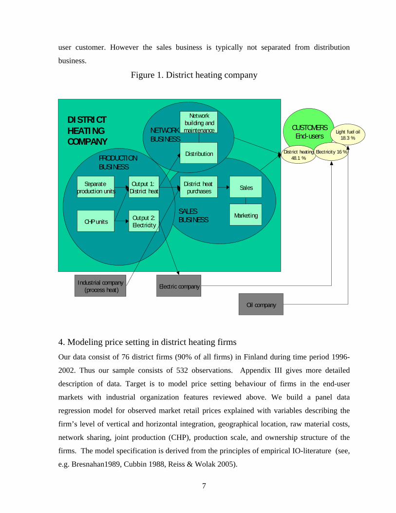
user customer. However the sales business is typically not separated from distribution

business.

Figure 1. District heating company

DISTRICT HEATING COMPANY

Separate production units

CHP units

Output 1: District heat

Output 2:Electricity

PRODUCTION BUSINESS

Networkbuilding andmaintenance

Distribution

NETWORK BUSINESS

District heat purchases Sales

Marketing

Electric company

CUSTOMERSEnd-users

SALES BUSINESS

Industrial company(process heat)

District heating48.1 %

Light fuel oil18.3 %

Electricity 16 %

Oil company

4. Modeling price setting in district heating firms Our data consist of 76 district firms (90% of all firms) in Finland during time period 1996-

2002. Thus our sample consists of 532 observations. Appendix III gives more detailed

description of data. Target is to model price setting behaviour of firms in the end-user

markets with industrial organization features reviewed above. We build a panel data

regression model for observed market retail prices explained with variables describing the

firm’s level of vertical and horizontal integration, geographical location, raw material costs,

network sharing, joint production (CHP), production scale, and ownership structure of the

firms. The model specification is derived from the principles of empirical IO-literature (see,

e.g. Bresnahan1989, Cubbin 1988, Reiss & Wolak 2005).

7

The variables are defined as

Price variables:

= price of district heating for small (single) family houses (€/kWt) ,SMA

i tP

,APA

i tP = price of district heating for apartment houses (€/kWt)

Vertical and horizontal integration variables:

,MSi tPROD = firm’s market share in district heat production (0-100%)

,MSi tSMALL = firm’s market share in energy retail markets of

small family houses (0-100%) ,

MSi tAPART = firm’s market share in energy retail markets of

apartment houses (0-100%) = dummy variable for joint production of electricity and heat ,i tCHP (1 = joint production, 0 = heat production) ,i tJOINT = dummy variable for joint retail selling of electricity and heat (1 = joint retail selling, 0 = only heat selling) = number of wholesale suppliers that the retail seller has (0,1,..,N) ,i jSUPPLY = dummy variable of distribution network sharing ,i tNETWORK (1 = firm shares network other firms, 0 = no sharing) *) Geographical location: ,i tLOCATION = dummy variable for firm’s geographical location reflecting the local raw material dependency (0=south, 1=coast, 2= east and north) *) Ownership: = dummy variable for firm’s ownership (1 = public, 0 = private) ,i tPUBLIC = dummy variable for firm’s ownership structure (1 = part of ,i tCOMPANY larger company, 0 = not part of larger company) Firm’s scale: = the scale of production or retail selling of district heat (GWt) ,i tSCALE ____________________________ *) These variables were connected together as two-dimensional dummy variable, , describing dependency between firm’s location and network sharing (see kmD Appendix I for more details)

8

Input costs: ,i tFUELCOST = the unit cost of fuel input of producer company (if the company is sole retail seller or distribution company variable gets the value of this company’s major heat supplier) Competition:

1999

0, when 1999

1, when 1999t

TRLt<⎧

= ⎨ ≥⎩

= a trend level shift variable that describes the price effect of

deregulation of Finnish energy markets starting in year 1999.

Our base line model has the from of (expect that , 1MS

i tAPART − is used instead of , 1MSi tSMALL − for

apartment house specification)

2 1, 0 , 1 0 * 19990 0

1 , 1 2 , 1

3 , 4 , 5 , 6 , 7

8 , 9

j ji t i i t km km tk m

MS MSi t i t

i t i t i t i t i t

i t

P P a D TR TRL

PROD SMALL

CHP JOINT SUPPLY PUBLIC COMPANY

SCALE FUELCOS

α β δ δ

β β

β β β β β

β β

− = =

− −

= + + + +

+ +

+ + + + +

+ +

∑ ∑

, , ,

where 1, 2,...,6, 1, 2,..,76, and small or apartment house.

ji t i tT u

t i j

+

= = =

,

TRt in a common time trend variable for all firms describing the common time depended

price effects. One period lagged endogeneous variable is also included in the model as price

dynamics are quite slow in district heating retail markets. Typically the firms change their

prices only on yearly basis. Notice also that market share variables are lagged with one

period. The price setting is one strategic variable in rivalry for market shares. Now the lagged

share variables exclude the effects from prices to market shares. Thus the used specification

is not sensitive to endogeneity specification bias. Note that we use also GMM –estimation

method in panel setting (Arellano 2003). In this case market share variables are not lagged

9

with one period but we use instrumental variable estimation method (i.e. GMM) to solve the

endogeneity problem. iα is the firm specific (fixed or random) component that models the

unobserved firm heterogeneity. Finally uit is normally and independently distributed error

term with common variance, 2(0, )it uu N σ∼ .

We estimate different specifications of above model in pooled and panel data settings

emphasizing the time dependent policy changes in the sample period, and regional network

sharing classifying price effects (see Appendix II for different specifications). In order

to study more closely the network-sharing effects the model was augmented with interaction

terms between and other right hand side variables (excluding ’s and

kmD

,i tNETWORK kmD

, 1j

i tP − ). This specification enables us to test if the possible network-sharing effects are only

location specific or they have more general pricing effects, i.e. the network-sharing firms’

pricing policy with respect to their market and production structure imply different energy

prices compared to non network-sharing firms.

5. Results 5.1. Small house pricing

We first pay attention to regional differences in pricing. Table 1a. reports the standard OLS

model estimates and interaction OLS-model estimates for pooled data. Results indicate that

there exist regional price differences for small houses. The estimates for D00,...,D21 show

tendency that firms located in the Eastern or Northern Finland (D20,D21), using mainly

wood and peat based material input in heat production, have the lowest retail energy prices.

However if the firm is a distribution network-sharing firm (Di1, i=01,2) this does not lower

the price. Notice that this result does not mean that price differences between network-

sharing and non-network-sharing firms are non-existing. The parameter equality tests for

estimates of D00,...,D21 in Tables 1b-1c. indicate clearly that relevant pricing differences are

found among the firms depending on their geographical location and network-sharing

possibilities. However there are no systematic differences over the regions for network-

sharing. Note that the “long run” level estimates of D00,...,D21 are obtained by adjusting the

estimates with the price dynamics estimate, e.g. D00LR=9.34/(1-0.77) = 40.6. Appendix IV

10

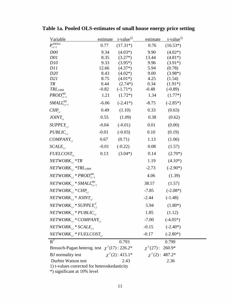
Table 1a. Pooled OLS-estimates of small house energy price setting Variable estimate t-value1) estimate t-value1)

, 1SMALL

i tP − 0.77 (17.31*) 0.76 (16.53*) D00 9.34 (4.03*) 9.90 (4.02*) D01 8.35 (3.27*) 13.44 (4.81*) D10 9.33 (3.95*) 9.96 (3.91*) D11 12.66 (4.37*) 5.94 (0.78) D20 8.43 (4.02*) 9.00 (3.98*) D21 8.75 (4.01*) 4.25 (1.54) TR 0.44 (2.74*) 0.34 (1.91*) TRL1999 -0.82 (-1.71*) -0.48 (-0.89)

, 1MSi tPROD − 1.21 (1.72*) 1.34 (1.77*)

, 1MSi tSMALL − -6.06 (-2.41*) -8.75 (-2.85*)

,i tCHP 0.49 (1.10) 0.33 (0.63)

,i tJOINT 0.55 (1.09) 0.38 (0.62)

,i jSUPPLY -0.04 (-0.01) 0.01 (0.00)

,i tPUBLIC -0.01 (-0.03) 0.10 (0.19)

,i tCOMPANY 0.67 (0.71) 1.13 (1.06)

,i tSCALE -0.01 (-0.22) 0.08 (1.57)

,i tFUELCOST 0.13 (3.04*) 0.14 (2.70*)

,i tNETWORK *TR 1.19 (4.10*)

,i tNETWORK *TRL1999 -2.73 (-2.90*)

,i tNETWORK * , 1MSi tPROD − 4.06 (1.39)

,i tNETWORK * , 1MSi tSMALL − 38.57 (1.57)

,i tNETWORK * -7.85 (-2.08*) ,i tCHP

,i tNETWORK * ,i tJOINT -2.44 (-1.48)

,i tNETWORK * 5.94 (1.80*) ,F

i jSUPPLY

,i tNETWORK * 1.85 (1.12) ,i tPUBLIC

,i tNETWORK * -7.00 (-4.05*) ,i tCOMPANY

,i tNETWORK * -0.15 (-2.40*) ,i tSCALE

,i tNETWORK * ,i tFUELCOST -0.17 (-2.80*)

R2 0.793 0.799

Breusch-Pagan heterog. test : 226.2* : 260.9* 2 (17)χ 2 (27)χ BJ normality test : 415.1* : 487.2* 2 (2)χ 2 (2)χ Durbin Watson test 2.43 2.36 1) t-values corrected for heteroskedasticity *) significant at 10% level

11

Table 1b. Tests for equality of distribution network-sharing and regional specific effects (p-values in parenthesis)

Overall equality: D00=D10=D20= D01=D11=D21

Regional equality: D00=D10=D20, D01=D11=D21

Network sharing / non sharing equality: D00=D01,D10=D11,D20=D21

2 (5) 16.92 (0.005)χ =

2 (4) 14.26 (0.006)χ =

2 (3) 13.16 (0.004)χ =

Table 1c. Tests for equality of distribution network sharing and regional specific effects in interaction model (p-values in parenthesis)

Overall equality: D00=D10=D20= D01=D11=D21

Regional equality: D00=D10=D20, D01=D11=D21

Network sharing / non sharing equality: D00=D01,D10=D11,D20=D21

2 (5) 19.32 (0.001)χ =

2 (4) 8.73 (0.009)χ = 2 (3) 13.31 (0.004)χ =

reports the unbalanced panel estimation results where variables D00,...,D21 build up six

regional-network specific cross sections in the panel setting. The estimation results are in

line with Table 1a. results but some positive price effects mount from the firm being part of

larger company.

Before analyzing in details the remaining results we notice that our estimation results are

greatly harmed by residual heteroskedasticity and non-normality. The firm level hetero-

geneity of our sample is not controlled in the OLS-model estimation for pooled data. To

secure consistent t-values we used heteroskedasticity consistent standard errors (White’s

diagonal moment matrix correction).

The second part of Table 1. reports the results from interaction model where we let network-

sharing dummy to interact with explanatory variables. The specification reveals the

differences between network-sharing and non network-sharing firms’ energy pricing

explained by the “structural” variables. The results indicate that network-sharing firms react

differently to these variables compared to non-sharing firms. Generally the pricing effects

among the network-sharing firms are amplified but some network-sharing firm specific

12

effects are also found, e.g. joint production of electricity and heat among the network-

sharing firms ( * - variable) decreases energy prices. Likewise if the

firms is part of larger company ( * ), and if the production scale of

firm is large ( * ) the energy prices are lower. However contrary to

theoretical arguments, the number of wholesale suppliers *

increases, and the unit cost of fuel input of network-sharing producer company

* ) depresses prices.

,i tNETWORK ,i tCHP

,i tNETWORK ,i tCOMPANY

,i tNETWORK ,i tSCALE

,( i tNETWORK , )i jSUPPLY

,( i tNETWORK ,i tFUELCOST

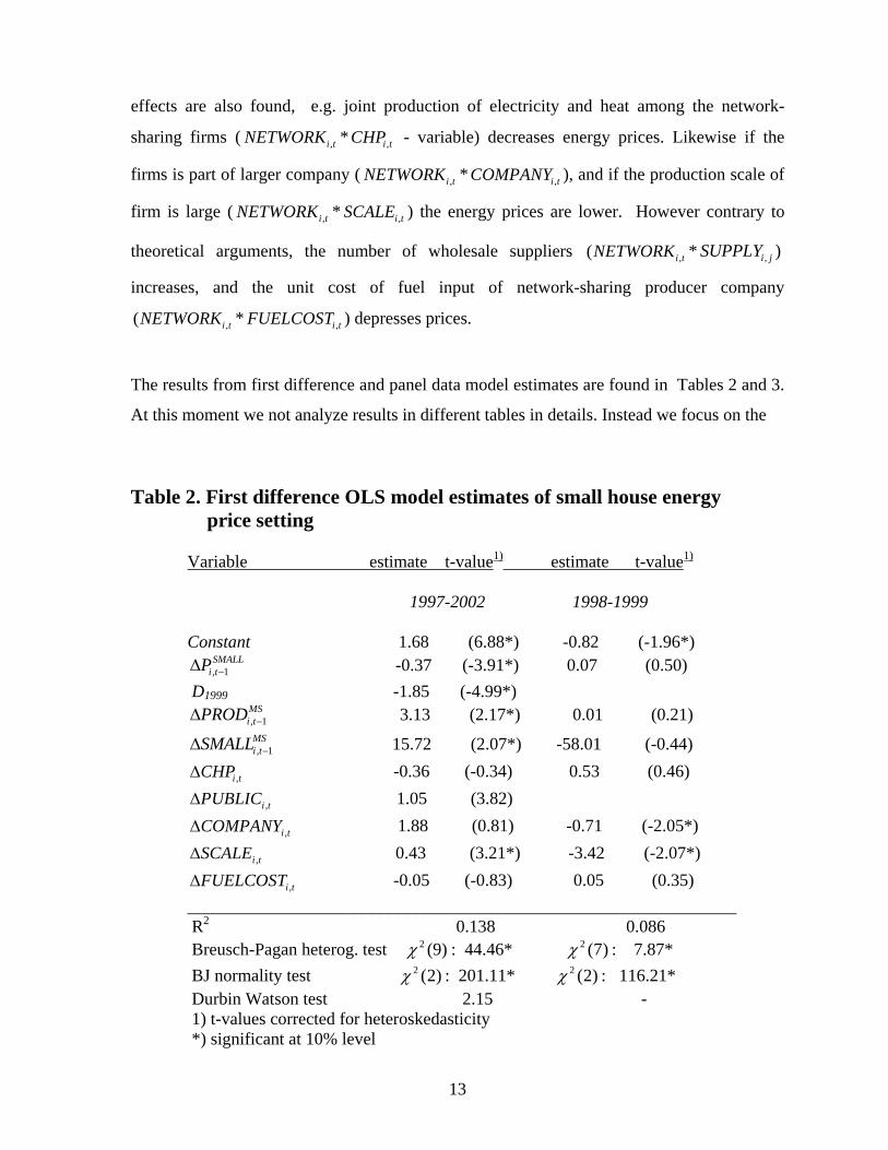
The results from first difference and panel data model estimates are found in Tables 2 and 3.

At this moment we not analyze results in different tables in details. Instead we focus on the

Table 2. First difference OLS model estimates of small house energy price setting

Variable estimate t-value1) estimate t-value1)

1997-2002 1998-1999 Constant 1.68 (6.88*) -0.82 (-1.96*)

, 1SMALL

i tP −Δ -0.37 (-3.91*) 0.07 (0.50) D1999 -1.85 (-4.99*)

, 1MSi tPROD −Δ 3.13 (2.17*) 0.01 (0.21)

, 1MSi tSMALL −Δ 15.72 (2.07*) -58.01 (-0.44)

,i tCHPΔ -0.36 (-0.34) 0.53 (0.46)

,i tPUBLICΔ 1.05 (3.82)

,i tCOMPANYΔ 1.88 (0.81) -0.71 (-2.05*)

,i tSCALEΔ 0.43 (3.21*) -3.42 (-2.07*)

,i tFUELCOSTΔ -0.05 (-0.83) 0.05 (0.35) _______________________________________________________________ R2

0.138 0.086 Breusch-Pagan heterog. test : 44.46* : 7.87* 2 (9)χ 2 (7)χ BJ normality test : 201.11* : 116.21* 2 (2)χ 2 (2)χ Durbin Watson test 2.15 - 1) t-values corrected for heteroskedasticity *) significant at 10% level

13

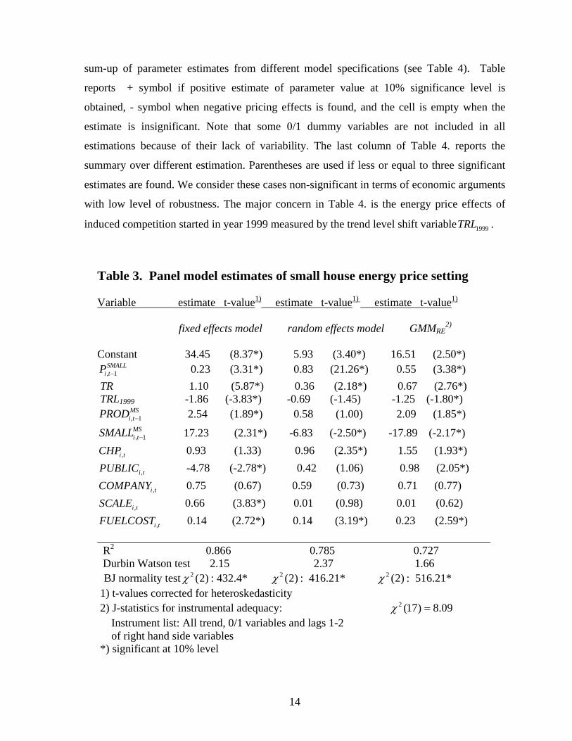
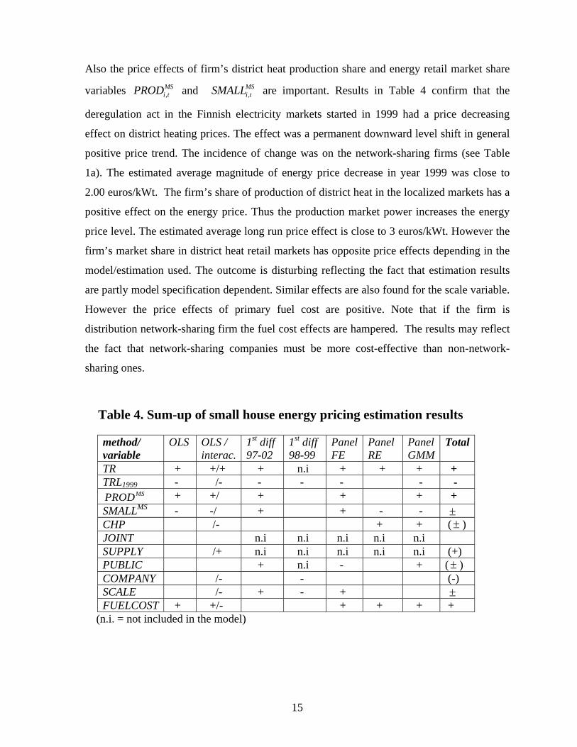
sum-up of parameter estimates from different model specifications (see Table 4). Table

reports + symbol if positive estimate of parameter value at 10% significance level is

obtained, - symbol when negative pricing effects is found, and the cell is empty when the

estimate is insignificant. Note that some 0/1 dummy variables are not included in all

estimations because of their lack of variability. The last column of Table 4. reports the

summary over different estimation. Parentheses are used if less or equal to three significant

estimates are found. We consider these cases non-significant in terms of economic arguments

with low level of robustness. The major concern in Table 4. is the energy price effects of

induced competition started in year 1999 measured by the trend level shift variable . 1999TRL

Table 3. Panel model estimates of small house energy price setting Variable estimate t-value1) estimate t-value1) estimate t-value1)

fixed effects model random effects model GMMRE

2)

Constant 34.45 (8.37*) 5.93 (3.40*) 16.51 (2.50*)

, 1SMALL

i tP − 0.23 (3.31*) 0.83 (21.26*) 0.55 (3.38*) TR 1.10 (5.87*) 0.36 (2.18*) 0.67 (2.76*) TRL1999 -1.86 (-3.83*) -0.69 (-1.45) -1.25 (-1.80*)

, 1MSi tPROD − 2.54 (1.89*) 0.58 (1.00) 2.09 (1.85*)

, 1MSi tSMALL − 17.23 (2.31*) -6.83 (-2.50*) -17.89 (-2.17*)

,i tCHP 0.93 (1.33) 0.96 (2.35*) 1.55 (1.93*)

,i tPUBLIC -4.78 (-2.78*) 0.42 (1.06) 0.98 (2.05*)

,i tCOMPANY 0.75 (0.67) 0.59 (0.73) 0.71 (0.77)

,i tSCALE 0.66 (3.83*) 0.01 (0.98) 0.01 (0.62)

,i tFUELCOST 0.14 (2.72*) 0.14 (3.19*) 0.23 (2.59*) ______________________________________________________________________ R2

0.866 0.785 0.727 Durbin Watson test 2.15 2.37 1.66

BJ normality test : 432.4* : 416.21* : 516.21* 2 (2)χ 2 (2)χ 2 (2)χ 1) t-values corrected for heteroskedasticity 2) J-statistics for instrumental adequacy: 2 (17) 8.09 χ = Instrument list: All trend, 0/1 variables and lags 1-2 of right hand side variables *) significant at 10% level

14

Also the price effects of firm’s district heat production share and energy retail market share

variables ,MSi tPROD and ,

MSi tSMALL are important. Results in Table 4 confirm that the

deregulation act in the Finnish electricity markets started in 1999 had a price decreasing

effect on district heating prices. The effect was a permanent downward level shift in general

positive price trend. The incidence of change was on the network-sharing firms (see Table

1a). The estimated average magnitude of energy price decrease in year 1999 was close to

2.00 euros/kWt. The firm’s share of production of district heat in the localized markets has a

positive effect on the energy price. Thus the production market power increases the energy

price level. The estimated average long run price effect is close to 3 euros/kWt. However the

firm’s market share in district heat retail markets has opposite price effects depending in the

model/estimation used. The outcome is disturbing reflecting the fact that estimation results

are partly model specification dependent. Similar effects are also found for the scale variable.

However the price effects of primary fuel cost are positive. Note that if the firm is

distribution network-sharing firm the fuel cost effects are hampered. The results may reflect

the fact that network-sharing companies must be more cost-effective than non-network-

sharing ones.

Table 4. Sum-up of small house energy pricing estimation results

method/ variable

OLS OLS / interac.

1st diff 97-02

1st diff 98-99

PanelFE

Panel RE

Panel GMM

Total

TR + +/+ + n.i + + + + TRL1999 - /- - - - - -

MSPROD + +/ + + + + SMALLMS - -/ + + - - ±CHP /- + + ( ) ±JOINT n.i n.i n.i n.i n.i SUPPLY /+ n.i n.i n.i n.i n.i (+) PUBLIC + n.i - + ( ) ±COMPANY /- - (-) SCALE /- + - + ±FUELCOST + +/- + + + +

(n.i. = not included in the model)

15

The rest of results in Table 4. lack stability and robustness. However if we overvalue the

results we notice that firm being part of larger company has a price depressing effect. Also if

the firm production structure allows for CHP-production it is expected to have negative price

effects. This result is confirmed by OLS-estimation and -stratification panel estimation

results found in Appendix IV. However a firm selling both electricity and heat has no retail

price effects.

kmD

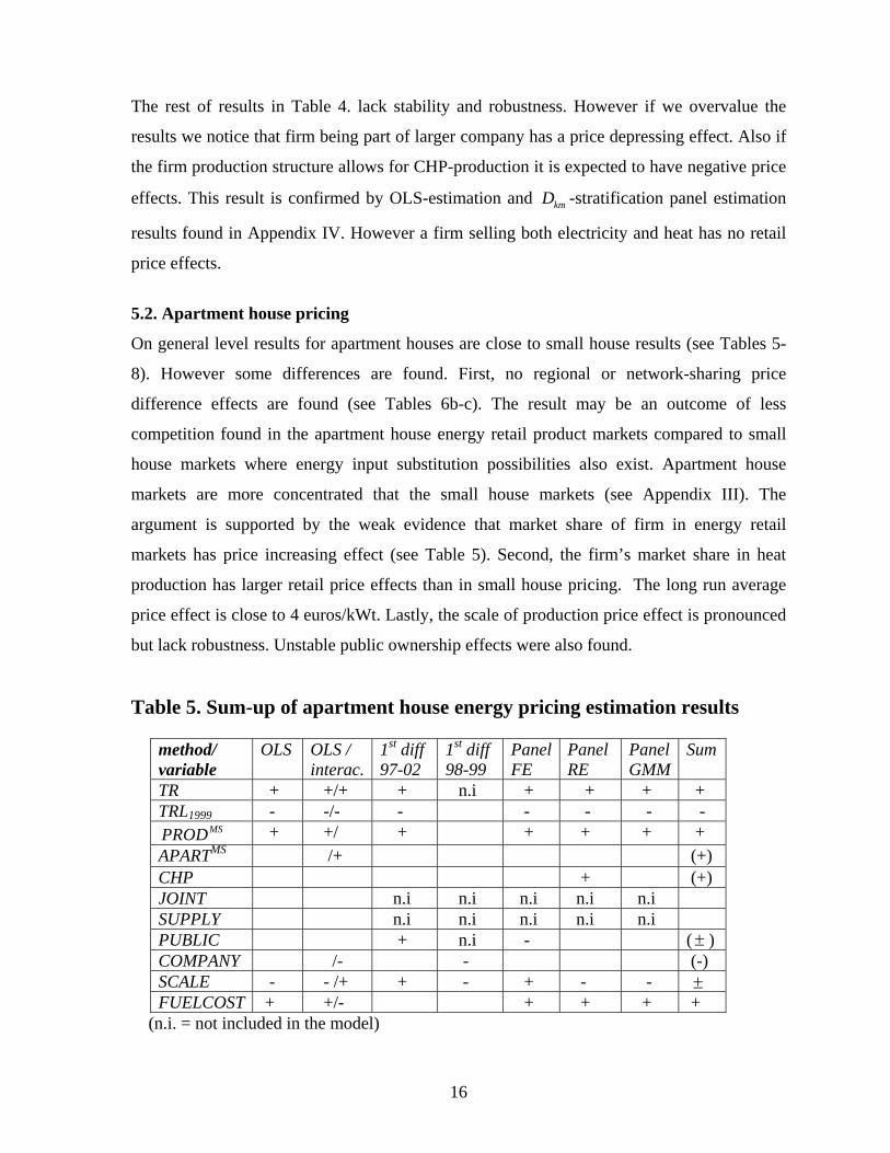
5.2. Apartment house pricing

On general level results for apartment houses are close to small house results (see Tables 5-

8). However some differences are found. First, no regional or network-sharing price

difference effects are found (see Tables 6b-c). The result may be an outcome of less

competition found in the apartment house energy retail product markets compared to small

house markets where energy input substitution possibilities also exist. Apartment house

markets are more concentrated that the small house markets (see Appendix III). The

argument is supported by the weak evidence that market share of firm in energy retail

markets has price increasing effect (see Table 5). Second, the firm’s market share in heat

production has larger retail price effects than in small house pricing. The long run average

price effect is close to 4 euros/kWt. Lastly, the scale of production price effect is pronounced

but lack robustness. Unstable public ownership effects were also found.

Table 5. Sum-up of apartment house energy pricing estimation results

method/ variable

OLS OLS / interac.

1st diff 97-02

1st diff 98-99

PanelFE

Panel RE

Panel GMM

Sum

TR + +/+ + n.i + + + + TRL1999 - -/- - - - - -

MSPROD + +/ + + + + + APARTMS /+ (+) CHP + (+) JOINT n.i n.i n.i n.i n.i SUPPLY n.i n.i n.i n.i n.i PUBLIC + n.i - ( ) ±COMPANY /- - (-) SCALE - - /+ + - + - - ±FUELCOST + +/- + + + +

(n.i. = not included in the model)

16

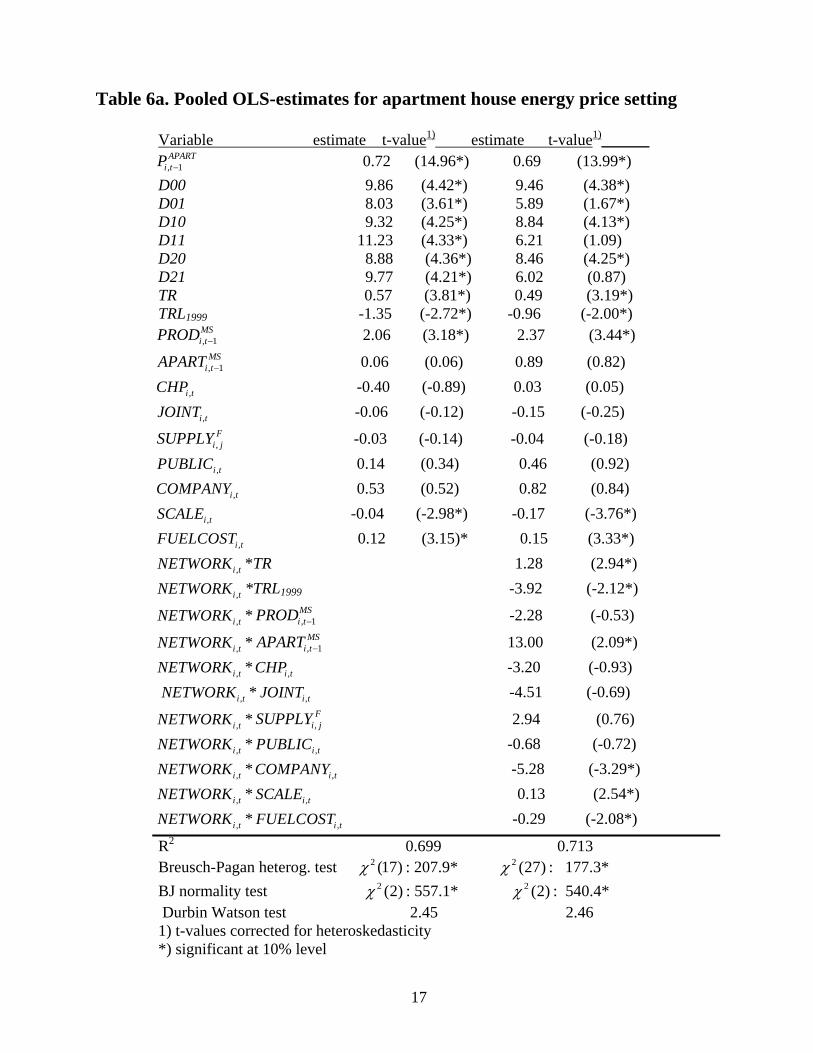
Table 6a. Pooled OLS-estimates for apartment house energy price setting

Variable estimate t-value1) estimate t-value1)______ , 1APART

i tP − 0.72 (14.96*) 0.69 (13.99*) D00 9.86 (4.42*) 9.46 (4.38*) D01 8.03 (3.61*) 5.89 (1.67*) D10 9.32 (4.25*) 8.84 (4.13*) D11 11.23 (4.33*) 6.21 (1.09) D20 8.88 (4.36*) 8.46 (4.25*) D21 9.77 (4.21*) 6.02 (0.87) TR 0.57 (3.81*) 0.49 (3.19*) TRL1999 -1.35 (-2.72*) -0.96 (-2.00*)

, 1MSi tPROD − 2.06 (3.18*) 2.37 (3.44*)

, 1MS

i tAPART − 0.06 (0.06) 0.89 (0.82)

,i tCHP -0.40 (-0.89) 0.03 (0.05)

,i tJOINT -0.06 (-0.12) -0.15 (-0.25)

,F

i jSUPPLY -0.03 (-0.14) -0.04 (-0.18)

,i tPUBLIC 0.14 (0.34) 0.46 (0.92)

,i tCOMPANY 0.53 (0.52) 0.82 (0.84)

,i tSCALE -0.04 (-2.98*) -0.17 (-3.76*)

,i tFUELCOST 0.12 (3.15)* 0.15 (3.33*)

,i tNETWORK *TR 1.28 (2.94*)

,i tNETWORK *TRL1999 -3.92 (-2.12*)

,i tNETWORK * , 1MSi tPROD − -2.28 (-0.53)

,i tNETWORK * , 1MS

i tAPART − 13.00 (2.09*)

,i tNETWORK * -3.20 (-0.93) ,i tCHP *,i tNETWORK ,i tJOINT -4.51 (-0.69)

,i tNETWORK * 2.94 (0.76) ,F

i jSUPPLY

,i tNETWORK * -0.68 (-0.72) ,i tPUBLIC

,i tNETWORK * -5.28 (-3.29*) ,i tCOMPANY

,i tNETWORK * 0.13 (2.54*) ,i tSCALE

,i tNETWORK * -0.29 (-2.08*) ,i tFUELCOST

R2 0.699 0.713

Breusch-Pagan heterog. test : 207.9* : 177.3* 2 (17)χ 2 (27)χ BJ normality test : 557.1* : 540.4* 2 (2)χ 2 (2)χ Durbin Watson test 2.45 2.46 1) t-values corrected for heteroskedasticity *) significant at 10% level

17

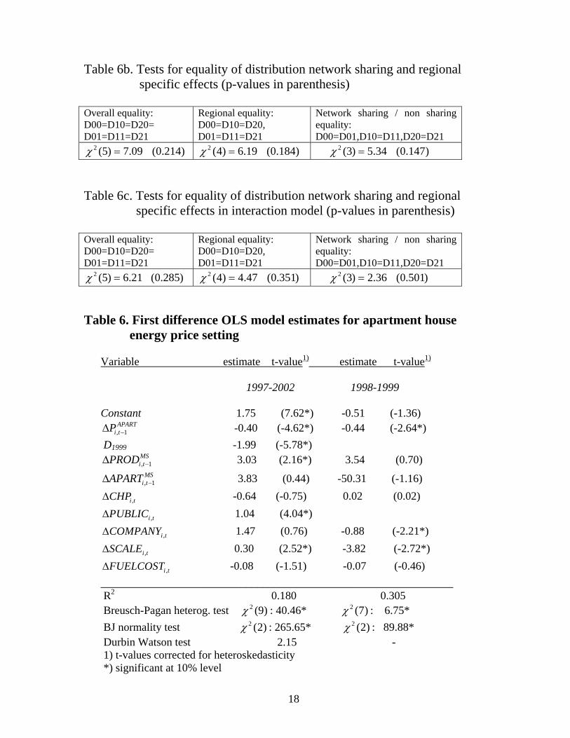
Table 6b. Tests for equality of distribution network sharing and regional specific effects (p-values in parenthesis) Overall equality: D00=D10=D20= D01=D11=D21

Regional equality: D00=D10=D20, D01=D11=D21

Network sharing / non sharing equality: D00=D01,D10=D11,D20=D21

2 (5) 7.09 (0.214)χ = 2 (4) 6.19 (0.184)χ = 2 (3) 5.34 (0.147)χ = Table 6c. Tests for equality of distribution network sharing and regional specific effects in interaction model (p-values in parenthesis) Overall equality: D00=D10=D20= D01=D11=D21

Regional equality: D00=D10=D20, D01=D11=D21

Network sharing / non sharing equality: D00=D01,D10=D11,D20=D21

2 (5) 6.21 (0.285)χ = 2 (4) 4.47 (0.351)χ = 2 (3) 2.36 (0.501)χ = Table 6. First difference OLS model estimates for apartment house energy price setting

Variable estimate t-value1) estimate t-value1)

1997-2002 1998-1999 Constant 1.75 (7.62*) -0.51 (-1.36)

, 1APART

i tP −Δ -0.40 (-4.62*) -0.44 (-2.64*) D1999 -1.99 (-5.78*)

, 1MSi tPROD −Δ 3.03 (2.16*) 3.54 (0.70)

, 1MS

i tAPART −Δ 3.83 (0.44) -50.31 (-1.16)

,i tCHPΔ -0.64 (-0.75) 0.02 (0.02)

,i tPUBLICΔ 1.04 (4.04*)

,i tCOMPANYΔ 1.47 (0.76) -0.88 (-2.21*)

,i tSCALEΔ 0.30 (2.52*) -3.82 (-2.72*)

,i tFUELCOSTΔ -0.08 (-1.51) -0.07 (-0.46) _______________________________________________________________ R2

0.180 0.305 Breusch-Pagan heterog. test : 40.46* : 6.75* 2 (9)χ 2 (7)χ BJ normality test : 265.65* : 89.88* 2 (2)χ 2 (2)χ Durbin Watson test 2.15 - 1) t-values corrected for heteroskedasticity *) significant at 10% level

18

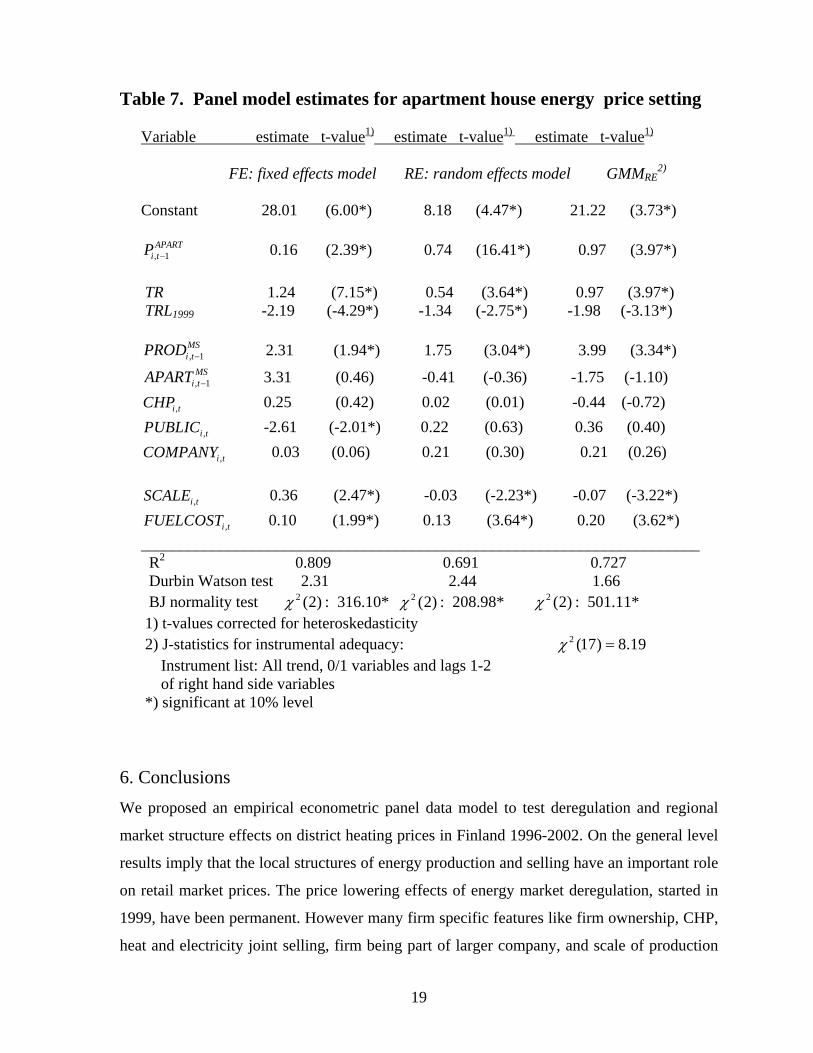
Table 7. Panel model estimates for apartment house energy price setting

Variable estimate t-value1) estimate t-value1) estimate t-value1)

FE: fixed effects model RE: random effects model GMMRE

2)

Constant 28.01 (6.00*) 8.18 (4.47*) 21.22 (3.73*)

, 1APART

i tP − 0.16 (2.39*) 0.74 (16.41*) 0.97 (3.97*) TR 1.24 (7.15*) 0.54 (3.64*) 0.97 (3.97*) TRL1999 -2.19 (-4.29*) -1.34 (-2.75*) -1.98 (-3.13*)

, 1MSi tPROD − 2.31 (1.94*) 1.75 (3.04*) 3.99 (3.34*)

, 1MS

i tAPART − 3.31 (0.46) -0.41 (-0.36) -1.75 (-1.10)

,i tCHP 0.25 (0.42) 0.02 (0.01) -0.44 (-0.72)

,i tPUBLIC -2.61 (-2.01*) 0.22 (0.63) 0.36 (0.40)

,i tCOMPANY 0.03 (0.06) 0.21 (0.30) 0.21 (0.26)

,i tSCALE 0.36 (2.47*) -0.03 (-2.23*) -0.07 (-3.22*)

,i tFUELCOST 0.10 (1.99*) 0.13 (3.64*) 0.20 (3.62*) ______________________________________________________________________ R2

0.809 0.691 0.727 Durbin Watson test 2.31 2.44 1.66 BJ normality test : 316.10* : 208.98* : 501.11* 2 (2)χ 2 (2)χ 2 (2)χ 1) t-values corrected for heteroskedasticity 2) J-statistics for instrumental adequacy: 2 (17) 8.19 χ = Instrument list: All trend, 0/1 variables and lags 1-2 of right hand side variables *) significant at 10% level

6. Conclusions We proposed an empirical econometric panel data model to test deregulation and regional

market structure effects on district heating prices in Finland 1996-2002. On the general level

results imply that the local structures of energy production and selling have an important role

on retail market prices. The price lowering effects of energy market deregulation, started in

1999, have been permanent. However many firm specific features like firm ownership, CHP,

heat and electricity joint selling, firm being part of larger company, and scale of production

19

did not have unambiguous retail price effects. Although the main empirical results obtained

preserve robustness and theory corroboration the large unobserved firm heterogeneity needs

in future research more attention.

The results showed also the housing type dependency. For small house district heat markets

regional and distribution network sharing aspects are important but for apartment houses they

are not. However for both house types, the market shares of local district heat production

firms correlate positively with retail prices. The price effects of retail market shares of energy

selling firms were not confirmed. A firm sharing a distribution network with other companies

has stronger pricing effects with firm specific control variables than a non-sharing firm.

Some network sharing firm specific effects were also found.

From the policy perspective of market deregulation and industry restructuring the results are

encouraging. The electricity market restructuring started in 1999, affecting district heating

markets only indirectly, has lowered district heat housing prices. At the same time firm

market shares – especially in wholesale markets - have still non-competitive price effects. As

the district heating markets are highly localized with extended dependency, the market

deregulation and industry restructuring may be impossible. Stronger regulation and market

monitoring by the authorities may also in future be the only policy alternative.

20

References Arellano, M. (2003). Panel Data Econometrics, OUP. Bresnahan, T.F. (1989). Empirical Studies of Industries with Market Power, in Schmalensee, R. & Willig, R. (Eds.) Handbook of Industrial Organization Vol.II., Ch. 17. North- Holland, Amsterdam. Borenstein, S., Bushnell, J.B. & Wolak, F.A. (2002). “Measuring Market Inefficiencies in California’s Restructured Wholesale Electricity Markets”, American Economic Review 92, 1376-405. Cavanagh, R. & Sostelie, R. (1988) “Energy Distribution Monopolies: A Vision for the Next Century”, The Electricity Journal, August/September. Cubbin, J.S. (1988). Market Structure and Performance - The Empirical Research. Harwood Academic Publishers. London. Harris, C. (2006). Electricity Markets. Pricing, Structures and Economics, Wiley. NY. Iossa, E. (1999) “Informative Externalities and Pricing in Regulated Multi-Product Industries”, Journal of Industrial Economics 54, 159-219. Janse, J., Jeon, D.-S. & Menicucci, D.(2007) ”The Organization of Regulated Production: Complementaries, Correlation and Collusion”, forthcoming in International Journal of Industrial Organization. Laffont, J.-J. & Martimort,D. (1997) “Collusion under Asymmetric Infromation” Econometrica 65, 875-911. __________________(2000) “Mechanism Design with and Collusion and Correlation” Econometrica 68, 309-342. Reiss,P.C. & Wolak, F.A. (2005) “Structural Econometric Modeling: Rationales and Examples from Industrial Organization” prepared for Handbook of Econometrics, Vol.6. Tirole, J. (1989). The Theory of Industrial Organization, MIT Press. Waterson, M. (1984). Economic Theory of the Industry, CUP.Cambridge Wilson, R. (2002). “Architecture of Power Markets”, Econometrica 70, 1299-1340. Wooldridge, J.M. (2000). Introductory Econometrics. A Modern Approach, South-Western.

21

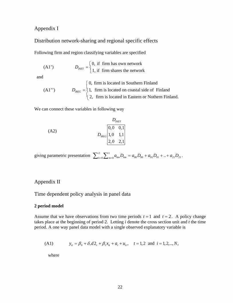
Appendix I Distribution network-sharing and regional specific effects Following firm and region classifying variables are specified

(A1’) 0, if firm has own network 1, if firm shares the network iNETD ⎧

= ⎨⎩

and

(A1’’) 0, firm is located in Southern Finland 1, firm is located on coastal side of Finland 2, firm is located in Eastern or Nothern Finland.

iREGD =⎧⎪⎨⎪⎩

We can connect these variables in following way

(A2)

0,0 0,11,0 1,12,0 2,1

iNET

iREG

D

D

giving parametric presentation . 2 1

00 00 01 01 21 210 0..km kmk m

a D a D a D a D= =

= + + +∑ ∑ Appendix II Time dependent policy analysis in panel data 2 period model Assume that we have observations from two time periods 1 and 2t t= = . A policy change takes place at the beginning of period 2. Letting i denote the cross section unit and t the time period. A one way panel data model with a single observed explanatory variable is (A1) 0 * 12 , 1, 2 and 1,2,.., ,it t it i ity d x a u t i Nβ δ β= + + + + = =

where

22

0, when 1 2 , and

1, when 2

measures cross section (unobserved) heterogeneity effects, and captures all other idiosyncratic and time-variyng unobserved effects.

t

i

it

td

t

au

=⎧= ⎨ =⎩

Thus at time period the intercept is 2t = 0 *β δ+ measuring the impact of policy change on the level of .ity Next if subtract the second period equation from the first, we obtain (A2) 2 1 * 1i i i i iy y y x uδ β− = Δ = + Δ + Δ , and read the policy effects form cross section OLS estimate of 0δ . This first-difference estimator has some advantages over the panel data model estimate (A1) since it has less parameters and consistency preserving condition for OLS, , disappears. If the cross section effects are of less importance the first difference model (A2) is a natural alternative for policy analysis (Wooldridge 2000).

( , ) 0i itCorr a x =

Multi-period model Typically we have a panel data with many time periods 1, 2,.., *,..,t t T= , where a policy change takes place at the beginning of period . Now a one way panel data model with p observed explanatory variables and year specific effects is

*t

(A3) 0 2 * 1

1

2 ... * ... ( 1)

, where 1,2,..., *,... and 1,2,.., , and

it t T t T t

pv vit i itv

y d dt d T dT

x a u t t T i N

β δ δ δ δ

β

−

=

= + + + + + − +

+ + + = =∑

0, when 1,

2,3,..., *,.... . 1, when , t

t t vdv v t T

t v= ≠⎧

= =⎨ =⎩

Difference model takes now from of

(A4) 2 * 1

1

2 ... * ... ( 1)

, 2,3,..., *,... and 1,2,.., .

it t T t T t

pv vit itv

y d dt d T dT

x u t t T i N

δ δ δ δ

β

−

=

Δ = Δ + + Δ + + Δ − + Δ

+ Δ + Δ = =∑

Model (A4) is problematic since it does not include a constant term and different yearly dummy variable takes different values in three year sequences. Likewise policy change year

23

*t is treated similarly like other years. One solution to these problems is the following difference model

(A5) 0 3 * 1

1

3 ... * .... ( 1)

, 2,3,..., *,... and 1,2,.., .

it t T t T t

pv vit itv

y d dt d T dT

x u t t T i N

β δ δ δ δ

β

−

=

Δ = + + + + + − +

+ Δ + Δ = =∑

A more efficient way to handle the policy issue is to use trend model like

(A6) 0 0 * * 1

,

1, 2,..., *,... and 1, 2,.., , and

pit t t v vit i itv

t

y TR TRL x a u

TR t T i N

β δ δ β=

= + + + + +

= =

∑

*

0, when *

1, when *. t

t tTRL

t t<⎧

= ⎨ ≥⎩ The specification in (A6) means that all time depended effects in ity are buried in a common time trend variable TRt and a trend level shift takes place at policy change year t*. Thus a trend break occurs at year t* without affecting the slope of trend. Now the difference model has a form

(A7) 0 * * 1

,

2,..., *,... and 1,2,.., , and

pit t v vit itv

y TRL x u

t t T i N

δ δ β=

Δ = + Δ + Δ + Δ

= =

∑

*

0, when *

1, when *. t

t tTRL

t t≠⎧

Δ = ⎨ =⎩ Thus the policy change year has its own specific, non permanent impulse, effect on *t t=

ityΔ , i.e. *δ , at year . *t Inserting the regional-network dummies in level model above leads to

24

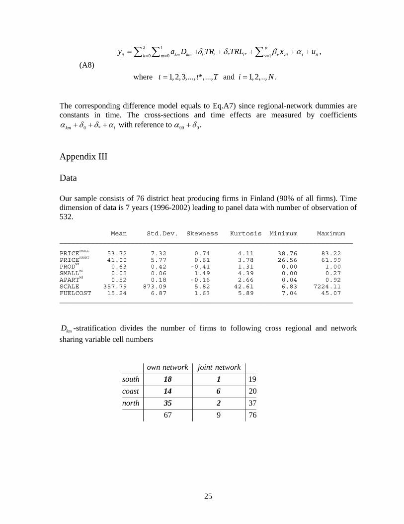
(A8)

2 10 * *0 0 1

,

where 1, 2,3,..., *,..., and 1,2,.., .

pit km km t t v vit i itk m v

y a D TR TRL x

t t T i N

δ δ β α= = =

= + + + +

= =

∑ ∑ ∑ u+

The corresponding difference model equals to Eq.A7) since regional-network dummies are constants in time. The cross-sections and time effects are measured by coefficients

0 * 00 0 with reference to .km iα δ δ α α δ+ + + + Appendix III Data Our sample consists of 76 district heat producing firms in Finland (90% of all firms). Time dimension of data is 7 years (1996-2002) leading to panel data with number of observation of 532. Mean Std.Dev. Skewness Kurtosis Minimum Maximum __________________________________________________________________________ PRICESMALL 53.72 7.32 0.74 4.11 38.76 83.22 PRICEAPART 41.00 5.77 0.61 3.78 26.56 61.99 PRODMS 0.63 0.42 -0.41 1.31 0.00 1.00 SMALLMS 0.05 0.06 1.49 4.39 0.00 0.27

APARTMS 0.52 0.18 -0.16 2.66 0.04 0.92 SCALE 357.79 873.09 5.82 42.61 6.83 7224.11 FUELCOST 15.24 6.87 1.63 5.89 7.04 45.07 __________________________________________________________________________

kmD -stratification divides the number of firms to following cross regional and network sharing variable cell numbers

192037

67 9 76

own network joint networksouthcoastnorth

18 114 635 2

25

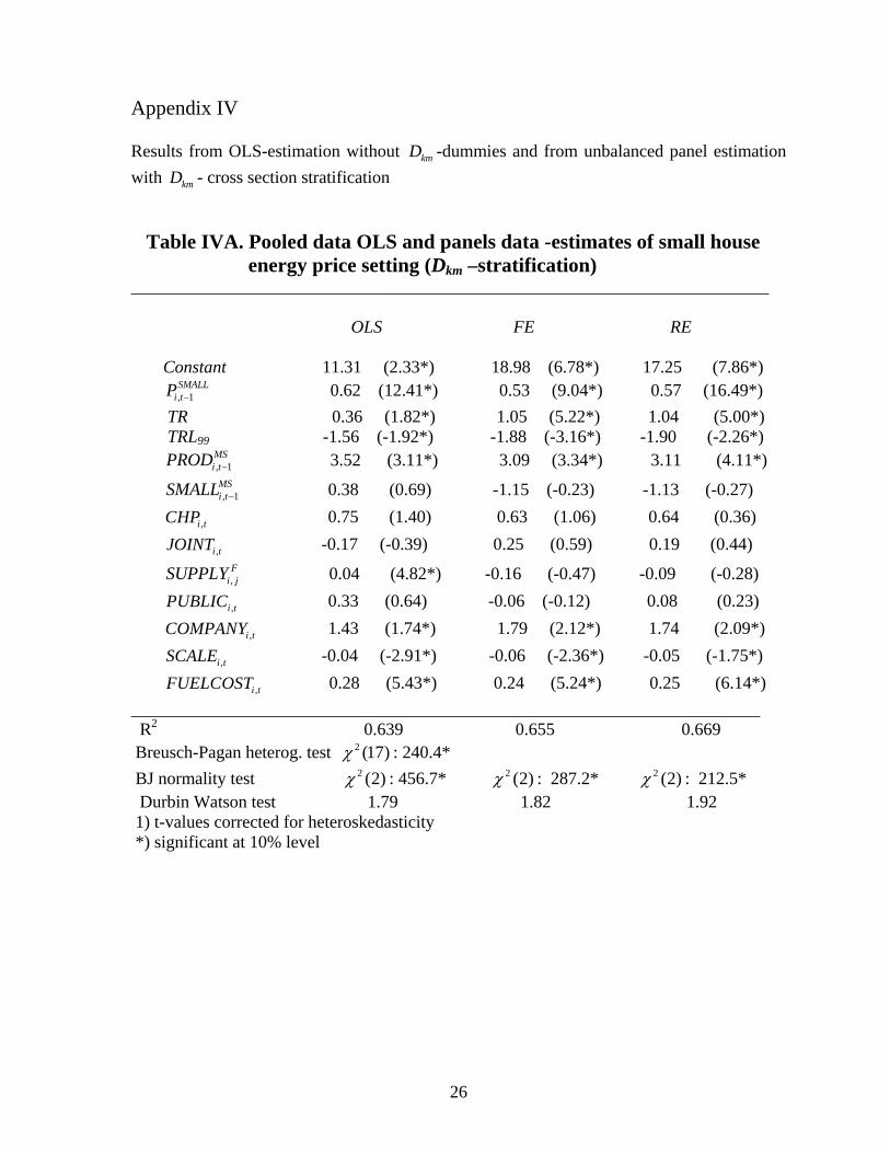
Appendix IV Results from OLS-estimation without -dummies and from unbalanced panel estimation with - cross section stratification

kmD

kmD Table IVA. Pooled data OLS and panels data -estimates of small house energy price setting (Dkm –stratification) _________________________________________________________________________

OLS FE RE Constant 11.31 (2.33*) 18.98 (6.78*) 17.25 (7.86*)

, 1SMALL

i tP − 0.62 (12.41*) 0.53 (9.04*) 0.57 (16.49*) TR 0.36 (1.82*) 1.05 (5.22*) 1.04 (5.00*) TRL99 -1.56 (-1.92*) -1.88 (-3.16*) -1.90 (-2.26*)

, 1MSi tPROD − 3.52 (3.11*) 3.09 (3.34*) 3.11 (4.11*)

, 1MSi tSMALL − 0.38 (0.69) -1.15 (-0.23) -1.13 (-0.27)

,i tCHP 0.75 (1.40) 0.63 (1.06) 0.64 (0.36)

,i tJOINT -0.17 (-0.39) 0.25 (0.59) 0.19 (0.44)

,F

i jSUPPLY 0.04 (4.82*) -0.16 (-0.47) -0.09 (-0.28)

,i tPUBLIC 0.33 (0.64) -0.06 (-0.12) 0.08 (0.23)

,i tCOMPANY 1.43 (1.74*) 1.79 (2.12*) 1.74 (2.09*)

,i tSCALE -0.04 (-2.91*) -0.06 (-2.36*) -0.05 (-1.75*) 0.28 (5.43*) 0.24 (5.24*) 0.25 (6.14*) ,i tFUELCOST

________________________________________________________________________ R2

0.639 0.655 0.669 Breusch-Pagan heterog. test : 240.4* 2 (17)χ BJ normality test : 456.7* : 287.2* : 212.5* 2 (2)χ 2 (2)χ 2 (2)χ Durbin Watson test 1.79 1.82 1.92 1) t-values corrected for heteroskedasticity *) significant at 10% level

26

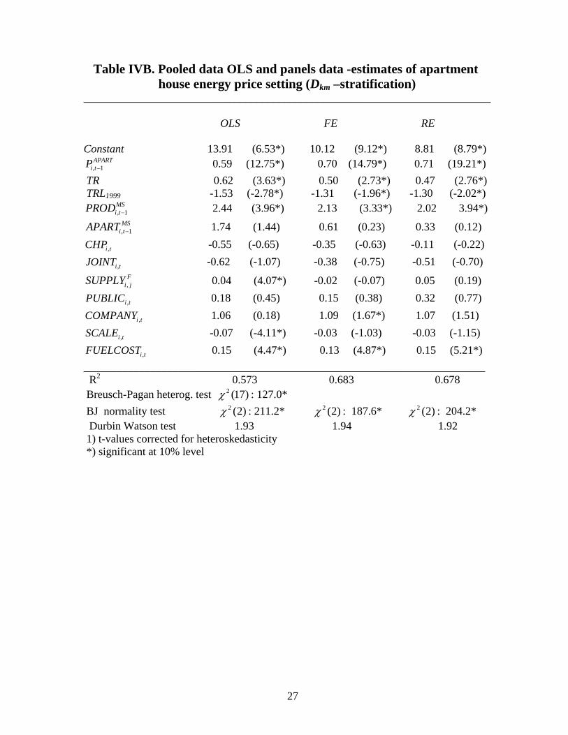
Table IVB. Pooled data OLS and panels data -estimates of apartment house energy price setting (Dkm –stratification) _________________________________________________________________________ OLS FE RE Constant 13.91 (6.53*) 10.12 (9.12*) 8.81 (8.79*)

, 1APART

i tP − 0.59 (12.75*) 0.70 (14.79*) 0.71 (19.21*) TR 0.62 (3.63*) 0.50 (2.73*) 0.47 (2.76*) TRL1999 -1.53 (-2.78*) -1.31 (-1.96*) -1.30 (-2.02*)

, 1MSi tPROD − 2.44 (3.96*) 2.13 (3.33*) 2.02 3.94*)

, 1MS

i tAPART − 1.74 (1.44) 0.61 (0.23) 0.33 (0.12)

,i tCHP -0.55 (-0.65) -0.35 (-0.63) -0.11 (-0.22)

,i tJOINT -0.62 (-1.07) -0.38 (-0.75) -0.51 (-0.70)

,F

i jSUPPLY 0.04 (4.07*) -0.02 (-0.07) 0.05 (0.19)

,i tPUBLIC 0.18 (0.45) 0.15 (0.38) 0.32 (0.77)

,i tCOMPANY 1.06 (0.18) 1.09 (1.67*) 1.07 (1.51)

,i tSCALE -0.07 (-4.11*) -0.03 (-1.03) -0.03 (-1.15)

,i tFUELCOST 0.15 (4.47*) 0.13 (4.87*) 0.15 (5.21*) ________________________________________________________________________ R2

0.573 0.683 0.678 Breusch-Pagan heterog. test : 127.0* 2 (17)χ BJ normality test : 211.2* : 187.6* : 204.2* 2 (2)χ 2 (2)χ 2 (2)χ Durbin Watson test 1.93 1.94 1.92 1) t-values corrected for heteroskedasticity *) significant at 10% level

27