Deregulated AGC scheme using Dynamic Programming Controller · 978-1-4799-5141-3/14/$31.00 ©2014...
6
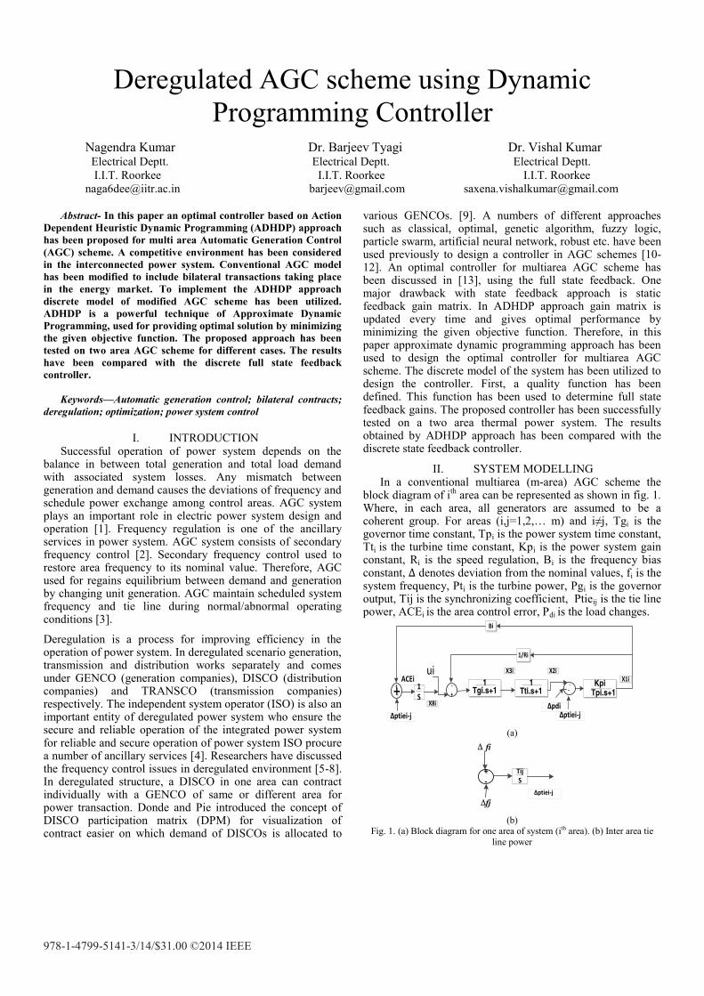
978-1-4799-5141-3/14/$31.00 ©2014 IEEE Deregulated AGC scheme using Dynamic Programming Controller Nagendra Kumar Dr. Barjeev Tyagi Dr. Vishal Kumar Electrical Deptt. Electrical Deptt. Electrical Deptt. I.I.T. Roorkee I.I.T. Roorkee I.I.T. Roorkee [email protected] [email protected] [email protected] Abstract- In this paper an optimal controller based on Action Dependent Heuristic Dynamic Programming (ADHDP) approach has been proposed for multi area Automatic Generation Control (AGC) scheme. A competitive environment has been considered in the interconnected power system. Conventional AGC model has been modified to include bilateral transactions taking place in the energy market. To implement the ADHDP approach discrete model of modified AGC scheme has been utilized. ADHDP is a powerful technique of Approximate Dynamic Programming, used for providing optimal solution by minimizing the given objective function. The proposed approach has been tested on two area AGC scheme for different cases. The results have been compared with the discrete full state feedback controller. Keywords—Automatic generation control; bilateral contracts; deregulation; optimization; power system control I. INTRODUCTION Successful operation of power system depends on the balance in between total generation and total load demand with associated system losses. Any mismatch between generation and demand causes the deviations of frequency and schedule power exchange among control areas. AGC system plays an important role in electric power system design and operation [1]. Frequency regulation is one of the ancillary services in power system. AGC system consists of secondary frequency control [2]. Secondary frequency control used to restore area frequency to its nominal value. Therefore, AGC used for regains equilibrium between demand and generation by changing unit generation. AGC maintain scheduled system frequency and tie line during normal/abnormal operating conditions [3]. Deregulation is a process for improving efficiency in the operation of power system. In deregulated scenario generation, transmission and distribution works separately and comes under GENCO (generation companies), DISCO (distribution companies) and TRANSCO (transmission companies) respectively. The independent system operator (ISO) is also an important entity of deregulated power system who ensure the secure and reliable operation of the integrated power system for reliable and secure operation of power system ISO procure a number of ancillary services [4]. Researchers have discussed the frequency control issues in deregulated environment [5-8]. In deregulated structure, a DISCO in one area can contract individually with a GENCO of same or different area for power transaction. Donde and Pie introduced the concept of DISCO participation matrix (DPM) for visualization of contract easier on which demand of DISCOs is allocated to various GENCOs. [9]. A numbers of different approaches such as classical, optimal, genetic algorithm, fuzzy logic, particle swarm, artificial neural network, robust etc. have been used previously to design a controller in AGC schemes [10- 12]. An optimal controller for multiarea AGC scheme has been discussed in [13], using the full state feedback. One major drawback with state feedback approach is static feedback gain matrix. In ADHDP approach gain matrix is updated every time and gives optimal performance by minimizing the given objective function. Therefore, in this paper approximate dynamic programming approach has been used to design the optimal controller for multiarea AGC scheme. The discrete model of the system has been utilized to design the controller. First, a quality function has been defined. This function has been used to determine full state feedback gains. The proposed controller has been successfully tested on a two area thermal power system. The results obtained by ADHDP approach has been compared with the discrete state feedback controller. II. SYSTEM MODELLING In a conventional multiarea (m-area) AGC scheme the block diagram of i th area can be represented as shown in fig. 1. Where, in each area, all generators are assumed to be a coherent group. For areas (i,j=1,2,… m) and i≠j, Tg i is the governor time constant, Tp i is the power system time constant, Tt i is the turbine time constant, Kp i is the power system gain constant, R i is the speed regulation, B i is the frequency bias constant, denotes deviation from the nominal values, f i is the system frequency, Pt i is the turbine power, Pg i is the governor output, Tij is the synchronizing coefficient, Ptie ij is the tie line power, ACE i is the area control error, P di is the load changes. 1 Tti.s+1 Kpi Tpi.s+1 1 Tgi.s+1 1/Ri Bi - + - + + 1 S Δptiei-j ui Δpdi Δptiei-j ACEi X2i X1i X3i X8i (a) Δptiei-j - + - + Tij S fj fi (b) Fig. 1. (a) Block diagram for one area of system (i th area). (b) Inter area tie line power
Transcript of Deregulated AGC scheme using Dynamic Programming Controller · 978-1-4799-5141-3/14/$31.00 ©2014...
978-1-4799-5141-3/14/$31.00 ©2014 IEEE
Deregulated AGC scheme using Dynamic
Programming ControllerNagendra Kumar Dr. Barjeev Tyagi Dr. Vishal Kumar Electrical Deptt. Electrical Deptt. Electrical Deptt.
I.I.T. Roorkee I.I.T. Roorkee I.I.T. Roorkee
[email protected] [email protected] [email protected]
Abstract- In this paper an optimal controller based on Action
Dependent Heuristic Dynamic Programming (ADHDP) approach
has been proposed for multi area Automatic Generation Control
(AGC) scheme. A competitive environment has been considered
in the interconnected power system. Conventional AGC model
has been modified to include bilateral transactions taking place
in the energy market. To implement the ADHDP approach
discrete model of modified AGC scheme has been utilized.
ADHDP is a powerful technique of Approximate Dynamic
Programming, used for providing optimal solution by minimizing
the given objective function. The proposed approach has been
tested on two area AGC scheme for different cases. The results
have been compared with the discrete full state feedback
controller.
Keywords—Automatic generation control; bilateral contracts;
deregulation; optimization; power system control
I. INTRODUCTION Successful operation of power system depends on the
balance in between total generation and total load demand with associated system losses. Any mismatch between generation and demand causes the deviations of frequency and schedule power exchange among control areas. AGC system plays an important role in electric power system design and operation [1]. Frequency regulation is one of the ancillary services in power system. AGC system consists of secondary frequency control [2]. Secondary frequency control used to restore area frequency to its nominal value. Therefore, AGC used for regains equilibrium between demand and generation by changing unit generation. AGC maintain scheduled system frequency and tie line during normal/abnormal operating conditions [3].
Deregulation is a process for improving efficiency in the operation of power system. In deregulated scenario generation, transmission and distribution works separately and comes under GENCO (generation companies), DISCO (distribution companies) and TRANSCO (transmission companies) respectively. The independent system operator (ISO) is also an important entity of deregulated power system who ensure the secure and reliable operation of the integrated power system for reliable and secure operation of power system ISO procure a number of ancillary services [4]. Researchers have discussed the frequency control issues in deregulated environment [5-8]. In deregulated structure, a DISCO in one area can contract individually with a GENCO of same or different area for power transaction. Donde and Pie introduced the concept of DISCO participation matrix (DPM) for visualization of contract easier on which demand of DISCOs is allocated to
various GENCOs. [9]. A numbers of different approaches such as classical, optimal, genetic algorithm, fuzzy logic, particle swarm, artificial neural network, robust etc. have been used previously to design a controller in AGC schemes [10-12]. An optimal controller for multiarea AGC scheme has been discussed in [13], using the full state feedback. One major drawback with state feedback approach is static feedback gain matrix. In ADHDP approach gain matrix is updated every time and gives optimal performance by minimizing the given objective function. Therefore, in this paper approximate dynamic programming approach has been used to design the optimal controller for multiarea AGC scheme. The discrete model of the system has been utilized to design the controller. First, a quality function has been defined. This function has been used to determine full state feedback gains. The proposed controller has been successfully tested on a two area thermal power system. The results obtained by ADHDP approach has been compared with the discrete state feedback controller.
II. SYSTEM MODELLING In a conventional multiarea (m-area) AGC scheme the
block diagram of ith
area can be represented as shown in fig. 1. Where, in each area, all generators are assumed to be a coherent group. For areas (i,j=1,2,… m) and i≠j, Tgi is the governor time constant, Tpi is the power system time constant, Tti is the turbine time constant, Kpi is the power system gain constant, Ri is the speed regulation, Bi is the frequency bias constant, denotes deviation from the nominal values, fi is the system frequency, Pti is the turbine power, Pgi is the governor output, Tij is the synchronizing coefficient, Ptieij is the tie line power, ACEi is the area control error, Pdi is the load changes.
1Tti.s+1
KpiTpi.s+1
1Tgi.s+1
1/Ri
Bi
-+
-+++ 1
S
Δptiei-j
ui
ΔpdiΔptiei-j
ACEiX2i
X1iX3i
X8i
(a)
Δptiei-j
-+-+
TijS
fj
fi
(b)
Fig. 1. (a) Block diagram for one area of system (ith area). (b) Inter area tie
line power
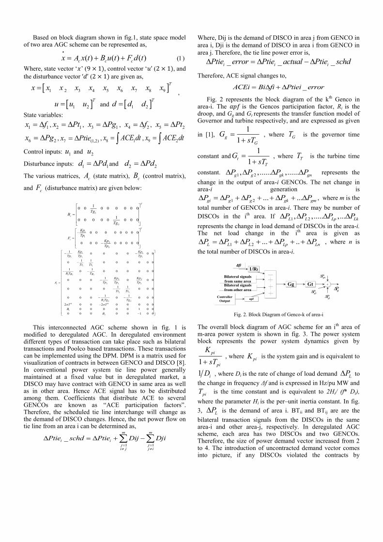
Based on block diagram shown in fig.1, state space model of two area AGC scheme can be represented as,
( ) ( ) ( )c c cx A x t B u t F d t
Where, state vector ‘ ’ ( , control vector ‘ ( , and
the disturbance vector ( are given as,
1 2 3 4 5 6 7 8 9
Tx x x x x x x x x x
,
1 2
Tu u u
and 1 2
Td d d
State variables:
1 1x f , 2 1x Pt , 3 1x Pg , 4 2x f , 5 2x Pt
6 2x Pg ,7 (1,2)x Ptie , 8 1x ACE dt , 9 2x ACE dt
Control inputs: 1u and 2u
Disturbance inputs: 1 1d Pd and 2 2d Pd
The various matrices, cA (state matrix), cB (control matrix),
and cF (disturbance matrix) are given below:
1
2
10 0 0 0 0 0 0 0
10 0 0 0 0 0 0 0
T
c
TgB
Tg
1
1
2
2
0 0 0 0 0 0 0 0
0 0 0 0 0 0 0 0
T
c
Kp
TpF
Kp
Tp
1 1
1 1 1
1 1
1 1 1
2 2
2 2 2
2 2
2 2 2
0 0
1
2
10 0 0 0 0 0
1 10 0 0 0 0 0 0
1 10 0 0 0 0 0 0
10 0 0 0 0 0
1 10 0 0 0 0 0 0
1 10 0 0 0 0 0 0
2 0 0 2 0 0 0 0 0
0 0 0 0 0 1 0 0
0 0 0 0 0 1 0 0
c
Kp Kp
Tp Tp Tp
Tt Tt
R Tg Tg
Kp Kp
Tp Tp TpA
Tt Tt
R Tg Tg
T T
B
B
This interconnected AGC scheme shown in fig. 1 is
modified to deregulated AGC. In deregulated environment different types of transaction can take place such as bilateral transactions and Poolco based transactions. These transactions can be implemented using the DPM. DPM is a matrix used for visualization of contracts in between GENCO and DISCO [8]. In conventional power system tie line power generally maintained at a fixed value but in deregulated market, a DISCO may have contract with GENCO in same area as well as in other area. Hence ACE signal has to be distributed among them. Coefficients that distribute ACE to several GENCOs are known as “ACE participation factors”. Therefore, the scheduled tie line interchange will change as the demand of DISCO changes. Hence, the net power flow on tie line from an area i can be determined as,
1 1
_m m
i i
j ji j j i
Ptie schd Ptie Dij Dji
Where, Dij is the demand of DISCO in area j from GENCO in
area i, Dji is the demand of DISCO in area i from GENCO in
area j. Therefore, the tie line power error is,
_ _ _i i iPtie error Ptie actual Ptie schd
Therefore, ACE signal changes to,
_ACEi Bi fi Ptiei error
Fig. 2 represents the block diagram of the kth
Genco in area-i. The is the Gencos participation factor, Ri is the droop, and Gg and Gt represents the transfer function model of Governor and turbine respectively, and are expressed as given
in [1], 1
1g
G
GsT
, where GT is the governor time
constant and1
1t
T
GsT
, where TT is the turbine time
constant. 1 2, ,...... ,......g g gk gnP P P P
represents the
change in the output of area-i GENCOs. The net change in area-i generation is
1 2 ... ...gi g g gk gmP P P P P , where m is the
total number of GENCOs in area-i. There may be number of
DISCOs in the ith
area. If 1 2, ,..... ,...L L Lp LkP P P P
represents the change in load demand of DISCOs in the area-i. The net load change in the i
th area is given as
1 2 ... ..L L L Lp LnP P P P P , where n is
the total number of DISCOs in area-i.
Controller
Output
1/Ri
apf
GtGg
Bilateral signals
from same area Bilateral signals
from other area
Δfi
1gP2gP
gmP
giP
Fig. 2. Block Diagram of Genco-k of area-i
The overall block diagram of AGC scheme for an ith
area of m-area power system is shown in fig. 3. The power system block represents the power system dynamics given by
1
pi
pi
K
sT , where
piK is the system gain and is equivalent to
1 iD , where Di is the rate of change of load demand LP to
the change in frequency Δf and is expressed in Hz/pu MW and
piT is the time constant and is equivalent to 2Hi/ (f* Di),
where the parameter Hi is the per–unit inertia constant. In fig.
3, LP is the demand of area i. BTii and BTij are are the
bilateral transaction signals from the DISCOs in the same area-i and other area-j, respectively. In deregulated AGC scheme, each area has two DISCOs and two GENCOs. Therefore, the size of power demand vector increased from 2 to 4. The introduction of uncontracted demand vector comes into picture, if any DISCOs violated the contracts by
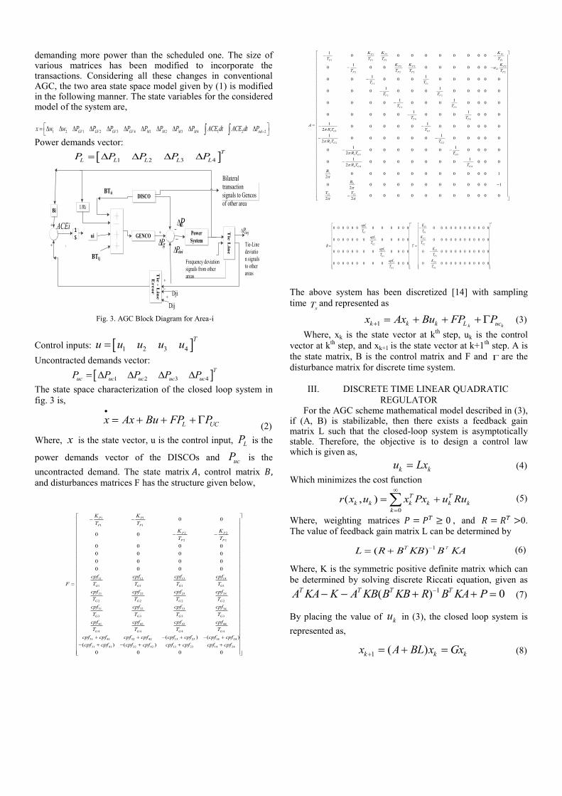
demanding more power than the scheduled one. The size of various matrices has been modified to incorporate the transactions. Considering all these changes in conventional AGC, the two area state space model given by (1) is modified in the following manner. The state variables for the considered model of the system are,
1 2 1 2 3 4 1 2 3 4 1 2 1 2GV GV GV GV M M M M tiex w w P P P P P P P P ACE dt ACE dt P
Power demands vector:
1 2 3 4
T
L L L L LP P P P P
Tie-Line
deviatio
n signals
to other
areas
Dij
GENCOPower
System
1/RiBi
DISCO
Tie
Lin
e
Tie
- L
ine
Erro
r
Frequency deviation
signals from other
areas
Bilateral
transaction
signals to Gencos
of other area
BTii
gP
LP
tieiPi
ACEi
BTij
Dji
tiejP
ui1S
Fig. 3. AGC Block Diagram for Area-i
Control inputs: 1 2 3 4
Tu u u u u
Uncontracted demands vector:
1 2 3 4
T
uc uc uc uc ucP P P P P
The state space characterization of the closed loop system in
fig. 3 is,
L UCx Ax Bu FP P
(2)
Where, x is the state vector, u is the control input, LP is the
power demands vector of the DISCOs and ucP is the
uncontracted demand. The state matrix , control matrix and disturbances matrices F has the structure given below,
1 1
1 1
2 2
2 2
1311 12 14
1 1 1 1
2321 22 24
2 2 2 2
31 32 33 34
3 3 3 3
4341 42 44
4 4 4 4
31 41 32 42
0 0
0 0
0 0 0 0
0 0 0 0
0 0 0 0
0 0 0 0
P P
P P
P P
P P
G G G G
G G G G
G G G G
G G G G
K K
T T
K K
T T
cpfcpf cpf cpf
T T T TF
cpfcpf cpf cpf
T T T T
cpf cpf cpf cpf
T T T T
cpfcpf cpf cpf
T T T T
cpf cpf cpf cpf
13 23 14 24
31 41 32 42 13 23 14 24
( ) ( )
( ) ( )
0 0 0 0
cpf cpf cpf cpf
cpf cpf cpf cpf cpf cpf cpf cpf
1 1 1
1 1 1 1
2 2 2
12
2 2 2 2
1 1
2 2
3 3
4 4
1 1 1
2 2 2
10 0 0 0 0 0 0 0 0
10 0 0 0 0 0 0 0 0
1 10 0 0 0 0 0 0 0 0 0 0
1 10 0 0 0 0 0 0 0 0 0 0
1 10 0 0 0 0 0 0 0 0 0 0
1 10 0 0 0 0 0 0 0 0 0 0
1 10 0 0 0 0 0 0 0 0 0 0
2
1 10 0 0 0 0 0 0 0 0 0
2
P P P
P P P P
P P P
P P P P
T T
T T
T T
T T
G G
G G
K K K
T T T T
K K Ka
T T T T
T T
T T
T T
T T
AR T T
R T T
3 3 3
4 4 4
1
2
12 12
0
1 10 0 0 0 0 0 0 0 0 0 0
2
1 10 0 0 0 0 0 0 0 0 0 0
2
0 0 0 0 0 0 0 0 0 0 0 12
0 0 0 0 0 0 0 0 0 0 0 12
0 0 0 0 0 0 0 0 0 0 02 2
G G
G G
R T T
R T T
B
B
T T
1 1
1 1
2 2
2 2
33
33
44
44
0 0 0 0 0 0 0 0 0 0 0 0 0 0 0 0 0 0 0 0 0 0 0 0
0 0 0 0 0 0 0 0 0 0 0 0 0 0 0 0 0 0 0 0 0 0 0 0
0 0 0 0 0 0 0 0 0 0 0 00 0 0 0 0 0 0 0 0 0 0 0
0 0 0 0 0 0 0 0 0 0 0 00 0 0 0 0 0 0 0 0 0 0 0
T
P
G P
P
G P
P
PG
P
PG
apf K
T T
apf K
T TB
Kapf
TT
Kapf
TT
T
The above system has been discretized [14] with sampling
time sT and represented as
1 k kk k k L ucx Ax Bu FP P (3)
Where, xk is the state vector at kth
step, uk is the control
vector at kth
step, and xk+1 is the state vector at k+1th
step. A is
the state matrix, B is the control matrix and F and are the
disturbance matrix for discrete time system.
III. DISCRETE TIME LINEAR QUADRATIC
REGULATOR For the AGC scheme mathematical model described in (3),
if (A, B) is stabilizable, then there exists a feedback gain matrix L such that the closed-loop system is asymptotically stable. Therefore, the objective is to design a control law which is given as,
k ku Lx (4)
Which minimizes the cost function
0
( , ) T T
k k k k k k
k
r x u x Px u Ru
(5)
Where, weighting matrices , and 0.
The value of feedback gain matrix L can be determined by
1( )TTL R B KB B KA (6)
Where, K is the symmetric positive definite matrix which can
be determined by solving discrete Riccati equation, given as 1( ) 0T T T TA KA K A KB B KB R B KA P (7)
By placing the value of ku in (3), the closed loop system is
represented as,
1 ( )k k kx A BL x Gx (8)
Where, G is the closed loop system matrix. Discrete state feedback controller is a static controller i.e., feedback gain matrix is constant. State feedback controller gives good dynamical responses, but determining the optimal control policies for nonlinear systems is difficult to solve analytically. It gives rise in complex state feedback or high order dynamical controller. The main limitation of the static controller is the risk of instability, since the gain matrix is static. ADHDP is an useful technique to design a dynamic feedback controller using approximate dynamic programming. This dynamic feedback controller can overcome the demerits of static feedback controller.
IV. ACTION DEPENDENT HEURISTIC DYNAMIC
PROGRAMMING (ADHDP) ADHDP is a useful technique of Approximate Dynamic
Programming (ADP), for feedback control of systems [14-17]. ADHDP, also known as Q- learning and used to estimate the Quality function, generally known as Q-function or action value function for any policy, optimal or non-optimal. In
ADHDP, first the feedback policy, i.e. kLx is evaluated and
then it is updated by utilizing Q function. Watkins [15] defined the Q function as a sum of the instantaneous cost incurred by taking action from state plus the total cost that would accrue if the fixed policy was followed from the state, mathematically this can be described as,
1( , ) ( , ) ( )k k k k kQ x u r x u V x (9)
Where, 0 1 is the discount factor. ( , )k kr x u is the
instantaneous cost and ( )kV x is the long term cost. For linear
system ( )kV x is quadratic and can be represented as,
( ) ( , ) ( )j k j k T T
k j j j j j i
j k j k
V x r x u x Px u Ru
0
( )i T T
i k i k i k i k
i
x Px u Ru
By placing the value of u and xk+1 from (4) and (8)
respectively, the total cost can be determined as (10), [14-15].
0
( )i T Ti k i k
i
x P L RL x
0
( ) ( ) ( )T i T i T i T
k k k k k
i
V x x D P L RL D x x Kx
(10)
For a linear system with quadratic cost, Q function also
becomes a quadratic function [16-17]. is set to 1 for
simplicity.
1 1 1
0( , ) ( , ) ( )
0
kT T T
k k k k k k k k k
k
xPQ x u r x u V x x u x Kx
uR
( ) ( )kT T T
k k k k k k
k
xx u G Ax Bu K Ax Bu
u
T
kT T
k k Tk
xAx u G K A B
uB
kT T
k k
k
xx u H
u
(11)
Where, 0
0
PG
R
is the block diagonal matrix with
blocks P and R, and ( )T
T
AH G K A B
B
is the
quadratic kernel matrix. Q function can be computed explicitly
for a Linear Quadratic Regulator (LQR) problem which is
quadratic in xk and uk and given as,
( , )xx xu kT T
k k k k
ux uu k
kT T
k k u
k
H H xQ x u x u
H H u
xx u H
u
(12)
Where x u is the column vector concatenation of and
, uH is a symmetric positive definite matrix, and the various
sub matrices are given in (13).
'
'
'
'
xx
ux
xu
uu
H P A KA
H A KB
H B KA
H R B KB
(13)
The sub matrix uuH is symmetric positive definite. By giving
policy and cost function at any time, an improved policy can
be determined as,
1 arg min ( , )k k k
u
L x Q x u (14)
Finally the minimum can be obtained by taking the partial
derivative of ( , )k kQ x u with respect to , setting it to zero.
, 0k k
k
Q x uu
(15)
By placing ( , )k kQ x u value from (12) in (15), control action
can be determined as,
1( )k uu ux ku H H x
0 ux k uu kH x H u (16)
Where, 1
1 ( )k uu uxL H H
is the minimizing policy for
all x. Further a new Q function can be assigned to the policy
and policy improvement procedure can be repeated. In
ADHDP technique, at each iteration gain matrix is updated
according to cost to provide the optimal policy. Therefore
ADHDP provides optimal policy for feedback control by
minimizing the given objective function or total cost.
V. RESULTS AND DISCUSSIONS To check the performance of the ADHDP controller two
area AGC scheme in deregulated scenario is considered. The parameters of AGC scheme are given in table I.
TABLE I. TWO AREA POWER SYSTEM PARAMETERS
( for both area)
governor time constant
s ( for both area)
power system time constant
( for both area)
power system gain constant
s ( for both area) turbine time constant
( for both area) speed regulation
( for both area) frequency bias constant
synchronizing constant
Two cases are considered in this work. In first case load
changes occur in area1 (DISCO1 and DISCO2) only. In first
case load changes occur in the DISCOs of both the areas. The
second case is a contract violation case where DISCO violates
the contract by demanding more power than specified in
contract.
A. Case 1 In this case 0.2 pu load demand change has been
considered in area1 (0.1 pu in DISCO1 and 0.1 pu in DISCO2), and 0.2 pu load demand change in area2 (0.1 pu in DISCO3 and 0.1 pu in DISCO4). All DISOCs have contract with GENCOs for power as per the following DPM.
0.5 0.25 0 0.3
0.2 0.25 0 0
0 0.25 1 0.7
0.3 0.25 0 0
DPM
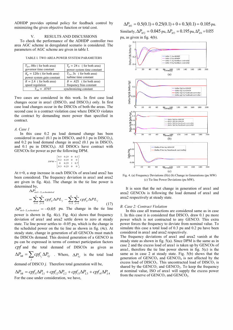
At t=0, a step increase in each DISCOs of area1and area2 has
been considered. The frequency deviation in area1 and area2
are given in fig. 4(a). The change in the tie line power is
determined by,
1 2,
2 4 4 2
1 3 3 1
tie scheduled
ij j ij j
i j i j
P
cpf PL cpf PL
(17)
1 2, 0.05tie scheduledP pu. The change in the tie line
power is shown in fig. 4(c). Fig. 4(a) shows that frequency
deviation of area1 and area2 settle down to zero at steady
state. Tie line power settles to -0.05 pu, which is the change in
the scheduled power on the tie line as shown in fig. (4c). At
steady state, change in generation of all GENCOs must match
the DISCOs demand. This desired generation of a GENCO in
pu can be expressed in terms of contract participation factors
cpf and the total demand of DISCOs as given as
jMi i Lj
j
P cpf P
. Where, LjP is the total load
demand of DISCO . Therefore total generation will be,
1 1 2 2 3 3 4 4Mi i L i L i L i LP cpf P cpf P cpf P cpf P
For the case under consideration, we have,
1 0.5(0.1) 0.25(0.1) 0 0.3(0.1) 0.105MP pu.
Similarly, 2 0.045MP pu, 3 0.195MP pu, 4 0.055MP
pu, as given in fig. 4(b).
(a)
(b)
(c)
Fig. 4. (a) Frequency Deviations (Hz) (b) Change in Generations (pu MW)
(c) Tie line Power Deviations (pu MW).
It is seen that the net change in generation of area1 and
area2 GENCOs is following the load demand of area1 and
area2 respectively at steady state.
B. Case 2: Contract Violation In this case all transactions are considered same as in case
1. In this case it is considered that DISCO1 draw 0.1 pu more power which is not contracted to any GENCO. This extra power forces the frequency to deviate from nominal value. To simulate this case a total load of 0.3 pu and 0.2 pu have been considered in area1 and area2 respectively. The frequency deviations of area1 and area2 vanish at the steady state as shown in fig. 5(a). Since DPM is the same as in case 2 and the excess load of area1 is taken up by GENCOs of area1, therefore the tie line power shown in fig. 5(c) is the same as in case 2 at steady state. Fig. 5(b) shows that the generation of GENCO3 and GENCO4 is not affected by the excess load of DISCO1. This uncontracted load of DISCO1 is shared by the GENCO1 and GENCO2. To keep the frequency at nominal value, ISO of area1 will supply the excess power from the reserve of GENCO1 and GENCO2.
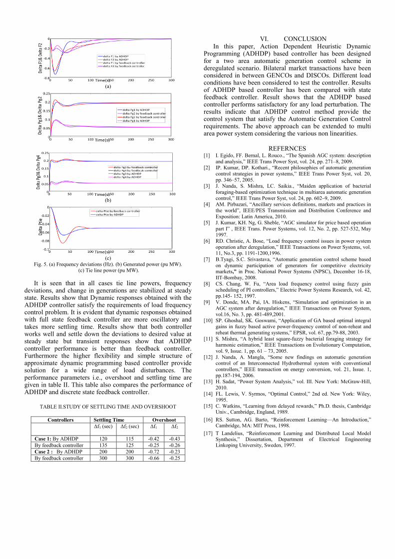
(a)
(b)
(c)
Fig. 5. (a) Frequency deviations (Hz). (b) Generated power (pu MW).
(c) Tie line power (pu MW).
It is seen that in all cases tie line powers, frequency deviations, and change in generations are stabilized at steady state. Results show that Dynamic responses obtained with the ADHDP controller satisfy the requirements of load frequency control problem. It is evident that dynamic responses obtained with full state feedback controller are more oscillatory and takes more settling time. Results show that both controller works well and settle down the deviations to desired value at steady state but transient responses show that ADHDP controller performance is better than feedback controller. Furthermore the higher flexibility and simple structure of approximate dynamic programming based controller provide solution for a wide range of load disturbances. The performance parameters i.e., overshoot and settling time are given in table II. This table also compares the performance of ADHDP and discrete state feedback controller.
TABLE II.STUDY OF SETTLING TIME AND OVERSHOOT
Controllers Settling Time Overshoot
Δf1 (sec) Δf2 (sec) Δf1
Δf2
Case 1: By ADHDP 120 115 -0.42 -0.43
By feedback controller 135 125 -0.25 -0.26
Case 2 : By ADHDP 200 200 -0.72 -0.23
By feedback controller 300 300 -0.66 -0.25
VI. CONCLUSION In this paper, Action Dependent Heuristic Dynamic
Programming (ADHDP) based controller has been designed for a two area automatic generation control scheme in deregulated scenario. Bilateral market transactions have been considered in between GENCOs and DISCOs. Different load conditions have been considered to test the controller. Results of ADHDP based controller has been compared with state feedback controller. Result shows that the ADHDP based controller performs satisfactory for any load perturbation. The results indicate that ADHDP control method provide the control system that satisfy the Automatic Generation Control requirements. The above approach can be extended to multi area power system considering the various non linearities.
REFERNCES [1] I. Egido, FF. Bernal, L. Rouco., “The Spanish AGC system: description
and analysis,” IEEE Trans Power Syst, vol. 24, pp. 271–8, 2009. [2] IP. Kumar, DP. Kothari., “Recent philosophies of automatic generation
control strategies in power systems,” IEEE Trans Power Syst, vol. 20,
pp. 346–57, 2005. [3] J. Nanda, S. Mishra, LC. Saikia., “Maiden application of bacterial
foraging-based optimization technique in multiarea automatic generation
control,” IEEE Trans Power Syst, vol. 24, pp. 602–9, 2009. [4] AM. Pirbazari, “Ancillary services definitions, markets and practices in
the world”, IEEE/PES Transmission and Distribution Conference and
Exposition: Latin America, 2010. [5] J. Kumar, KH. Ng, G. Sheble, “AGC simulator for price based operation
part I” , IEEE Trans. Power Systems, vol. 12, No. 2, pp. 527-532, May 1997.
[6] RD. Christie, A. Bose, “Load frequency control issues in power system
operation after deregulation,” IEEE Transactions on Power Systems, vol. 11, No.3, pp. 1191-1200,1996.
[7] B.Tyagi, S.C. Srivastava, “Automatic generation control scheme based
on dynamic participation of generators for competitive electricity
markets,” in Proc. National Power Systems (NPSC), December 16-18,
IIT-Bombay, 2008.
[8] CS. Chang, W. Fu, “Area load frequency control using fuzzy gain scheduling of PI controllers,” Electric Power Systems Research, vol. 42,
pp.145-/152, 1997.
[9] V. Donde, MA. Pai, IA. Hiskens, “Simulation and optimization in an AGC system after deregulation,” IEEE Transactions on Power System,
vol.16, No. 3, pp. 481-489,2001.
[10] SP. Ghoshal, SK. Goswami, “Application of GA based optimal integral gains in fuzzy based active power-frequency control of non-reheat and
reheat thermal generating systems,” EPSR, vol. 67, pp.79-88, 2003.
[11] S. Mishra, “A hybrid least square-fuzzy bacterial foraging strategy for harmonic estimation,” IEEE Transactions on Evolutionary Computation,
vol. 9, Issue. 1, pp. 61 – 73, 2005.
[12] J. Nanda, A. Mangla, “Some new findings on automatic generation control of an Interconnected Hydrothermal system with conventional
controllers,” IEEE transaction on energy conversion, vol. 21, Issue. 1,
pp.187-194, 2006.
[13] H. Sadat, “Power System Analysis,” vol. III. New York: McGraw-Hill,
2010.
[14] FL. Lewis, V. Syrmos, “Optimal Control,” 2nd ed. New York: Wiley, 1995.
[15] C. Watkins, “Learning from delayed rewards,” Ph.D. thesis, Cambridge Univ., Cambridge, England, 1989.
[16] RS. Sutton, AG. Barto, “Reinforcement Learning—An Introduction,” Cambridge, MA: MIT Press, 1998.
[17] T Landelius, “Reinforcement Learning and Distributed Local Model Synthesis,” Dissertation, Department of Electrical Engineering Linkoping University, Sweden, 1997.