DER-CAM User Manual - Building Microgrid full... · 5 I. Introduction to DER-CAM Web Optimization...

1

DER-CAM+ User Manual

Full DER Web Optimization Service: a project partly financed by

the U.S. Department of Energy

DER-CAM Version 5.0 (DER-CAM+).

Interface Version 2.1.12.

Copyright © LBNL 2008-2017

Lawrence Berkeley National Laboratory (LBNL)

03 – 20 – 2017

Project Scientific Lead: M. Stadler

Software design: D. Baldassari, T. Forget, M. Stadler, S. Wagner, F. Ewald

Optimization algorithm: G. Cardoso, S. Mashayekh, N. DeForest, M. Heleno, L. Le Gall, M. Hartner, C. Milan, T. Schittekatte, M. Stadler, D. Steen, J. Tjaeder

Special thanks to previous contributors

W. Feng, R. Firestone, J. Lai, C. Marnay, A. Siddiqui

This work was partly funded by the Public Interest Energy Research (PIER) program of the California Energy

Commission under California Interagency Agreement 500-02-004 to the California Institute for Energy and the

Environment (CIEE) and Memorandum Agreement POM081-L01 between The Regents of the University of

California and Lawrence Berkeley National Laboratory. The Berkeley Lab is managed and operated by the

University of California for the U.S. Department of Energy under contract DE-AC02-05CH11231.

2

Contents I. Introduction to DER-CAM Web Optimization ............................................................................................ 5

1. Key Concepts ......................................................................................................................................... 5

1.1. Key inputs of the model ................................................................................................................. 5

1.2. Outputs determined by DER-CAM ................................................................................................. 6

2. DER-CAM Web Optimization ................................................................................................................ 6

II. Getting started with DER-CAM in 5 Steps ................................................................................................. 7

1. Login (not applicable for Standalone version) ...................................................................................... 7

2. Review the Conditions .......................................................................................................................... 7

3. Create and Open Projects ..................................................................................................................... 7

3.1. New Project .................................................................................................................................... 7

3.2. Open an Existing Project ................................................................................................................ 7

4. Define Project Settings .......................................................................................................................... 8

4.1. Project name and DER-CAM versions ......................................................................................... 8

4.2. Single Node vs Multi-Node .......................................................................................................... 10

4.3. DER-CAM databases ..................................................................................................................... 11

4.4. View and modify project settings ................................................................................................ 13

5. Main screen overview ......................................................................................................................... 13

III. Overview of input parameters ............................................................................................................... 14

1. Global Settings .................................................................................................................................... 15

1.1. Investment Options (multi-node only) ..................................................................................... 15

1.2. Options Table ............................................................................................................................... 15

1.3. Parameters Table ......................................................................................................................... 15

1.4. Number of Days ........................................................................................................................... 17

2. Power Flow Parameters (multi-node only) ......................................................................................... 17

2.1. Options ........................................................................................................................................ 17

2.2. Parameters .................................................................................................................................. 18

2.3. Model 1 Parameters ................................................................................................................... 18

2.4. Model 2 Parameters ................................................................................................................... 18

2.5. Cable Parameters ........................................................................................................................ 19

2.6. Transformer Parameters ........................................................................................................... 19

3. Heat Transfer Parameters (multi-node only) ...................................................................................... 19

3

3.1. Options ........................................................................................................................................ 20

3.2. HT Pipe Parameters ................................................................................................................... 20

3.3. LT Pipe Parameters .................................................................................................................... 20

4. Site Weather Data ............................................................................................................................... 20

4.1. Solar Insulation ............................................................................................................................ 20

4.2. Ambient Hourly Temperature ...................................................................................................... 21

4.3. Other Location Data ..................................................................................................................... 21

4.4. Wind Power Potential .................................................................................................................. 21

5. Load Data ............................................................................................................................................ 22

5.1. Load (single node version) ........................................................................................................... 22

5.2. Load (multi node version) ............................................................................................................ 22

6. Utility ................................................................................................................................................... 23

6.1. Global Settings ............................................................................................................................. 23

6.2. Electricity Rates ............................................................................................................................ 24

6.3. Fuel Rates ..................................................................................................................................... 25

7. Technologies ....................................................................................................................................... 25

7.1. Single-node vs Multi-node versions ............................................................................................. 25

7.2. Global Tech Definitions ................................................................................................................ 25

7.3. Discrete Technologies .................................................................................................................. 26

7.4. Continuous Technologies ............................................................................................................. 27

8. Energy Management and Resiliency ................................................................................................... 28

8.1. Load Shifting ................................................................................................................................. 28

8.2. Demand Response ....................................................................................................................... 29

8.3. Direct Controllable Loads ............................................................................................................. 29

8.4. Resiliency...................................................................................................................................... 30

9. Advanced User Settings ...................................................................................................................... 31

9.1. Building Retrofit Settings ............................................................................................................. 31

9.2. Financial Incentives ...................................................................................................................... 32

9.3. SGIP .............................................................................................................................................. 32

10. Topology ............................................................................................................................................ 32

10.1. Create a new node ..................................................................................................................... 33

10.2. Node proprieties / Create new lines .......................................................................................... 33

4

10.3. Defining the load of the a consumption node ........................................................................... 33

10.4. Defining the Line, transformers and heat pipes parameters ..................................................... 34

IV. Case Study: single node version ............................................................................................................ 36

1. Starting the Project ............................................................................................................................. 36

2. Reference Case .................................................................................................................................... 36

3. Cost Minimization ............................................................................................................................... 43

4. CO2 Minimization ............................................................................................................................... 50

5. Multi-objective optimization .............................................................................................................. 52

6. Cost minimization with existing technologies, forced investments and grid outages ....................... 54

V. Case Study: multi-node version .............................................................................................................. 61

1. Starting the Project ............................................................................................................................. 61

2. Power Flow and Heat Transfer Parameters ........................................................................................ 61

3. Topology .............................................................................................................................................. 62

4. Load Database ..................................................................................................................................... 63

5. Reference Scenario ............................................................................................................................. 64

6. Investments Scenario .......................................................................................................................... 67

Appendix A: Assessments Levels for DER-CAM use .................................................................................... 72

1. Basic User Level ................................................................................................................................... 72

2. Intermediate User Level ...................................................................................................................... 72

3. Advanced User Level ........................................................................................................................... 73

4. Full User Level ..................................................................................................................................... 73

5

I. Introduction to DER-CAM Web Optimization This document contains the user manual for accessing DER-CAM via the Web Optimization

Interface in its current version, 5.0, and gives examples of its functionalities and options.

1. Key Concepts

What is DER-CAM?

DER-CAM (Distributed Energy Resources Customer Adoption Model) is a decision support

tool for investment and planning of distributed energy resources (DER) in buildings and

microgrids. The problem addressed by DER-CAM is formulated as a mixed integer linear

program (MILP) that finds optimal DER investments while minimizing total energy costs,

carbon dioxide (CO2) emissions, or a multi-objective combination of both criteria.

What is a Microgrid?

A microgrid is a group of interconnected loads and distributed energy resources within

clearly defined electrical boundaries that acts as a single controllable entity with respect to

the grid. A microgrid can connect and disconnect from the main grid and operate both in

grid-connected or island-mode. Distributed Energy Resources are commonly defined as a

set of locally available technologies and strategies with potential to make energy use more

efficient, accessible, and environmentally sustainable. These solutions include power

generation and combined heat and power (CHP) using conventional fuel-fired technologies,

but also renewable technologies such as PV, and energy management strategies such as

demand response, load shifting, and peak-shaving. Storage technologies, including

stationary storage, mobile storage in the form of electric vehicle batteries, as well as

thermal storage tanks, are also considered DER.

To optimize DER investments DER-CAM chooses the portfolio of technologies that

minimizes costs and/or environmental burdens, based on optimized hourly dispatch

decisions that consider specific site load, price information, and performance data for

available equipment options. The output results are composed of the optimal technology

portfolio and the corresponding dispatch profiles to achieve the optimal performance.

1.1. Key inputs of the model

a. Load Data - Customer's end-use hourly load profiles – ideally disaggregated by

major end-uses: e.g. space heat, hot water, natural gas only, (electric) cooling, (electric)

refrigeration, and electricity only . DER-CAM utilizes monthly load profiles three day-

types: week days, weekend days, and peak/outlier days.

6

b. Electricity Tariff and Fuel Costs - The structure and rates of the customer’s

electricity tariff, natural gas prices, and other relevant utility price data.

c. DER Technology Costs - Capital costs, operation and maintenance (O&M) costs,

along with fuel costs associated with the operation of various available technologies.

d. Investment Parameters - the discount rate on customer investment and maximum

allowed payback.

e. DER Technology Parameters - Basic technical performance indicators of

generation and storage technologies including the thermal-electric ratio that

determines the amount of residual heat that is available as a function of generator

electric output.

f. Network Topology - In case of multi-node microgrids, DER-CAM also considers the

energy networks models (electricity cables and gas/heat pipes characteristics) as well

as their operational limits, e.g. electricity network ampacities and voltage constraints or

heat/gas flows limits.

1.2. Outputs determined by DER-CAM

a. Optimal capacity of on-site DER in each node of the microgrid.

b. Optimized strategic dispatch of all DER, taking into account energy management

procedures.

c. Detailed economic results, including costs of energy supply and all DER related

costs.

2. DER-CAM Web Optimization

DER-CAM Web Optimization refers to the service that integrates the DER-CAM model with

a web-based user interface. This online platform facilitates the handling of input data and

optimization parameters prior to running the algorithm on a dedicated server hosted at

LBNL. It also enables graphical visualization of the results and exporting them via e-mail.

7

For simplicity, the DER-CAM Web Optimization will be referred to as DER-CAM throughout

this document. This manual is also valid for the “Standalone DER-CAM+” which can run

locally on a PC.

II. Getting started with DER-CAM in 5 Steps

In this section we will go through the very first steps to quickly setup a DER-CAM model.

1. Login (not applicable for Standalone version)

Go to https://microgrids2.lbl.gov and enter your user credentials. Click on “Login” and on the

following page click on “DER-CAM Plus”.

2. Review the Conditions

After the connection to the interface is established, a user agreement will appear. Please

review the conditions and click “Accept” to proceed or “Deny” to reject and exit the

application.

Note: At this point only advanced DER-CAM users are given a private storage folder for their DER-CAM projects

and customized versions. This can be accessed via the “Advanced user Login” button. For standard DER-CAM

access all files are currently kept in a common user folder and only the main stable version of DER-CAM is

offered. (Standalone version users always have private storage since it runs locally on a PC)

3. Create and Open Projects

3.1. New Project

On the main window (Figure 1) click on “New Project…” under “Start” to create a new DER-

CAM project. Alternatively you may click the button on the toolbar or select “New Project”

from the FILE menu.

3.2. Open an Existing Project

To open an existing project click on “Open Project…” under “Start”, use the button or select

“Open Project” from the FILE menu. To view and manage all your projects (rename, delete),

click on the VIEW menu and select “Your Projects”.

TIP: To create quickly a new project from an existing one, select “Save Project As…” in the File menu and enter a

name for your new project.

8

Figure 1: Start Window

4. Define Project Settings

4.1. Project name and DER-CAM versions

After selecting “New Project” the New Project window will appear (see Figure 2). Enter a

project name and select the DER-CAM version among the four options available: Basic,

Intermediate, Advanced and Full User.

A summary of the main input and output functionalities available in each version of the

DER-CAM is presented in the Table 1.

A full description of each version can be found in Appendix A.

9

DER-CAM Versions Enabled

Disabled

Functionalities Basic Intermediate Advanced Full User

Inp

uts

Scanning Databases

Editable Inputs (Loads, Solar

Radiation, Tariffs)

Microgrid outages (forced islanding)

Feed-in tariffs

Basic Load Management and

Resiliency Features

Advanced Load Management (Load

Shifting + Demand Response)

Full Customization of the microgrid

Building Retrofit Settings

Financial Settings

Zero Net Energy Constraint

Ou

tpu

ts

Run Base Case

Investment Analysis

Tradeoff analysis (outage costs vs

load curtailment/investments in DER)

Power Exports Scenarios

Islanding Scenarios

Results for real test sites (full

customizable microgrid)

Building Shell improvements

Performance and investment

subsidies

Net Metering and Zero Net Energy

Table 1: Overview of DER-CAM versions

10

Figure 2: New Project Window

4.2. Single Node vs Multi-Node

After selecting the DER-CAM version, the user is required to select single node or multi-

node microgrid model. In a single node model, all the load and DER resources of the

microgrid are considered to be connected to a single bus, which means that the energy

flows between the different locations within the microgrid are neglected. In contrast, the

multi-node model considers the electric, heat and gas networks of the microgrid and takes

into account, not only the type and size of the optimal DER investments, but also the

location of those investments. It is important to stress that the subsequent settings menus

that will be shown to the user will depend on this decision. Also, the type of DER-CAM

results presented for single-node and multi-node models will be different.

Table 2 summarizes the main differences between single node and multi-node models.

Main characteristics

Single node

Does not require information regarding network parameters. Faster total run-time. Ideal for small Microgrids or for situations where the networks parameters

are unknown

Multi-node Allows to optimize the location of the DER within the microgrid nodes Requires specific information about the microgrid gas, heat and electricity

network

11

Ideal for larger Microgrids and/or when the energy networks can be a limitations to the investment

Longer total run-time. Table 2: Single-node vs. multi-node

4.3. DER-CAM databases

DER-CAM includes three input databases to assist with the construction of new microgrid

projects, and also to illustrate the main inputs required by the tool. The databases comprise

Load Data; Solar Data and Tariff Data. Each database is composed of real data obtained for

specific locations outlined in the “New Project” window. As shown in Table 1, some

versions of the DER-CAM allow the user to modify these predefined values while building

the case. Use of each database can be enabled by ticking the corresponding checkbox.

a. Load Database:

Location information (e.g. country, state, and city), the type of building, and the period of

construction are required in order to get a load profile from the database. Once this is

provided and the data is loaded. Users may examine the loaded data by clicking on each of

the available tabs: “Electricity Only”, “Cooling”, “Refrigeration”, “Space Heating”, “Water

Heating”, “Natural Gas Only”. This navigation button show the disaggregated information

by the type of energy use. The slider on the right allows users to change the day-type

profile being displayed. Three types of day-type profiles are considered:

“Week” profile, comprising the average hourly consumption of the weekdays

“Weekend” profile, containing the average hourly consumption of the weekend day

“Peak” profile that is built considering the highest values registered for the hourly

consumption in each location.

These load profiles represent different consumption behaviors and are built assuming an

annual energy consumption of 1GWh. The magnitude of the profile can be scaled by using

the “Multiplier” boxes, located bellow the load data fields, where users can set the total

annual consumption of a specific site, and scale the load profiles accordingly.

More information about the Load Database is provided by clicking on the “Information on

load data” button. This will load the pop-up window shown in Figure 3, providing more

details about the assumptions and locations regarding the database.

The use of the load database in “New Project” window is not available if the multi-node

version is selected. For this version, the user is required to specify the load in each node of the

Microgrid network in the Parameters Menu (see section III.5.2).

12

Figure 3: Information on Load Data window

b. Solar Database:

Solar database provides irradiance values (in kW/square meter) for specific locations.

These are average values form the Typical Meteorological Year (TMY) collation. Besides the

location data (State and City) the user is required to select the TMY edition from which the

irradiance values should be extracted.

More information about the TMY editions are presented in a specific help widow (Figure 4)

that can be opened by clicking on “Information on solar data” button.

Figure 4: Information on Solar Data window

c. Tariff Database:

The tariffs available in DER-CAM database consist of a collection of data for each location

found in the DER-CAM Loads Database. In this database preparation, one utility was

selected in each location and three generalized tariffs were defined (small, medium and

large/industrial) to accommodate buildings with different peak loads. Thus, besides the

information about the location (State and City), the user must also select the appropriate

13

tariff based on the define load. More information about the three levels of tariff rates in

each location (Figure 5) can be obtained by clicking in “Information on Tariff Data”.

Figure 5: Information on Tariff data

4.4. View and modify project settings

Viewing and modifying the project settings can be done at any point during the session by

clicking on the “SETTINGS” menu.

5. Main screen overview

After creating a new project, you will be presented with the main screen. As shown in

Figure 6, this main panel is divided in three areas: Parameters Menu, Tables Input Area, and

Help Area. The Parameters Menu enables a hierarchical navigation through the parameters

required by DER-CAM. By selecting each category of inputs, the corresponding input table

will appear in the Table Area. Help information about the parameters will be presented in

the Help Area, on the right side of the panel. Finally, at the bottom of the screen, the

information regarding the DER-CAM version being used is displayed.

14

Figure 6: Input Main Screen

III. Overview of input parameters

In this section, we detail the type of inputs required by DER-CAM that should be specified

in the Parameters Menu. The Parameters Menu changes according to the type of microgrid

model selected by the user in the New Project menu, (single-node or multi-node.) For

each category of the Parameters menu explained bellow, we will indicate if it is associated

with the single-node and/or multi-node version of DER-CAM.

Parameters Menu

HelpWindow

DER-CAM Version

Input TablesArea

15

1. Global Settings

The Global Settings menu contains the general optimization parameters. It also includes the

main financial and technical parameters, as well as the high level options associated with

the technologies to be considered in the optimization. Three subsections are included

within Global Settings: Options Table; Parameter Table; Number of Days.

1.1. Investment Options (multi-node only)

The Investment Options Table is only available in multi-node version of DER-CAM. In this

table, the user can enable of disable the new investments in generation and storage

technologies per node of the microgrid, by setting 1 or 0, respectively, for each type of

investment.

1.2. Options Table

The Options Table is used to define key aspects in each model. It consists of a set of binary

parameters, where 0 disables and 1 enables the action controlled by that parameter. For

instance, setting “DiscreteInvest” to 1 will enable the possibility of investing in discrete

technologies, which consist of conventional distributed generation technologies modeled

internally using discrete variables. This includes reciprocating engines, microturbines, fuel-

cells, or gas turbines, as opposed to "continuous technologies", whose capacity is modeled

using continuous variables. This is an important distinction, as “Discrete technologies” can

only be installed in discrete quantities of the nameplate capacity. In contrast, the optimal

capacity of “Continuous technologies”, can be any continuous non-negative number. This

distinction is justified by the flexibility of commercially available system sizes.

Exporting generation can be enabled with the parameter “NonPVSales”, which allows for

the sale of generation from conventional DG technologies; and “PVSales”, which allows for

the sale of generation from PV. Revenue from export are determined using prices found in

the “PX Price” table under “Advanced User Settings.

The optimization objective function can also be selected in this menu. By default, DER-CAM

will minimize the economic function. Setting “MinimizeCO2” to 1 the objective will change

to CO2 minimization. Setting “MultiObjective” to 1 will select a weighted objective of both

costs and CO2 aspects will be considered.

1.3. Parameters Table

In the Parameter Table several project related global values can be set, including the key

financial parameters such as the project discount rate, the maximum payback period, and

16

the reference costs (base case cost) for investment scenarios. The reference costs represent

total annual energy costs prior to new investments in distributed generation technologies

and can be obtained by running DER-CAM only with the existing on-site technologies (if

any). It should be noted that even in the reference case DER-CAM will optimize the dispatch

of any existing DER, and, therefore, the reference case may already suggest relevant

improvements. The possibility of enabling existing technologies will be discussed in the

Technology section.

It is important to take into account that the “BaseCaseCost” is a key input of DER-CAM,

since it strongly relates to the maximum payback and, hence, it will affect the technology

portfolio that can be included in the optimal solution. The maximum payback constrain is

active in every investment run that is performed, and forces that any new investments

generate savings against the reference cost that respect a simple payback period shorter

than the maximum allowed payback time. In order to obtain a relevant estimation of

environmental performance, the CO2 emissions of the base case should also be introduced

in this table.

Furthermore, it should be noted that the maximum payback constraint is still active when

CO2 minimization is selected. For this reason, it may be necessary to either increase the

maximum payback period or increase the reference costs when looking for environmental

friendly solutions. This is not absolutely necessary, but failing to do so may lead to

solutions that have limited potential to reduce emissions.

If “MultiObjective” is being selected as the objective of the optimization, the solution found

by DER-CAM will lay between the cost optimal and CO2 optimal solutions, and the

preference over one objective or the other is determined by weighting factors

“MultiObjectiveWCosts” and “MultiObjectiveWCO2”. However, as both these objectives are

defined with different units, scaling factors must also be used.

To set the appropriate scaling factors, two separate optimization runs must be performed:

the scaling factor for costs, “MultiObjectiveMaxCosts”, is determined by performing a CO2

minimization and saving the correspondent cost. Similarly, the weighting factor for CO2,

“MultiObjectiveMaxCO2”, can be found by performing a cost minimization run and saving

the corresponding CO2 emissions. Although this is the recommended approach when using

weighted objectives, it should be noted that other procedures are possible and will

naturally impact the results. The weighted objective function used by DER-CAM is:

𝒎𝒊𝒏 𝒇 = 𝑴𝒖𝒍𝒕𝒊𝑶𝒃𝒋𝒆𝒄𝒕𝒊𝒗𝒆𝑾𝑪𝒐𝒔𝒕 ∗ (𝑻𝒐𝒕𝒂𝒍𝑨𝒏𝒏𝒖𝒂𝒍 𝑪𝒐𝒔𝒕

𝑴𝒖𝒍𝒕𝒊𝑶𝒃𝒋𝒆𝒄𝒕𝒊𝒗𝒆𝑴𝒂𝒙 𝑪𝒐𝒔𝒕)

+ 𝑴𝒖𝒍𝒕𝒊𝑶𝒃𝒋𝒆𝒄𝒕𝒊𝒗𝒆𝑾𝑪𝑶𝟐 ∗ (𝑻𝒐𝒕𝒂𝒍𝑨𝒏𝒏𝒖𝒂𝒍 𝑪𝑶𝟐

𝑴𝒖𝒍𝒕𝒊𝑶𝒃𝒋𝒆𝒄𝒕𝒊𝒗𝒆𝑴𝒂𝒙 𝑪𝑶𝟐)

17

An alternative method to explicitly take CO2 emissions into account in the optimization

process is through the ‘CO2tax’ value found in the Parameter Table and enabled through

the Options Table. This will introduce a price for the CO2 emissions in the costs objective

function of the DER-CAM.

In summary, performing investment runs in DER-CAM requires a reference case. If the

DER-CAM optimization is used with a single objective, a base case scenario with no

investments must be run in order to obtain the ‘BaseCaseCost’ and 'BaseCaseCO2'. Please

note that for this run you must specify the existing technologies without allowing any

further investments. In case of using the multi-objective formulation, two additional runs

are needed to determine 'MultiObjectiveMaxCosts' and 'MultiObjectiveCO2'. In chapter IV

of this Manual, a Case Study is conducted in order to illustrate the different uses of the DER-

CAM.

1.4. Number of Days

The “Number of Days” table provides the weight of each day-type per month to scale up to

a full year. Possible day types include week-days, weekend-days and peak-days, as well as

the emergency equivalents when considering outages. A more detailed description about

emergency days is given in the ‘Resiliency and Demand Management Section’. Please note

that the total number of days in this table must equal the number of days in a year, i.e.,

when defining emergency days the equivalent number must be subtracted from the

corresponding non-emergency day type.

2. Power Flow Parameters (multi-node only)

The power flow parameters section contains a set of tables that allow users to specify

options and parameters directly related with the electricity grid. It is important to stress

that this section of the menu is only available if the user selects the multi-node version of

DER-CAM in the “New Project” window (see section II.4.2).

2.1. Options

The Options table allows users to enable or disable the power flow constraints of the multi-

node optimization. By disabling this parameter the placement of DER technologies in the

network will be arbitrary since the network constraints are neglected. It is also possible to

select the type of power flow model used to represent the electricity network, by changing

18

the parameter “ModelNo”. Currently, DER-CAM offers two options for this parameter,

Model 1 and Model 2.

Model 1 is based on the linear formulation proposed in: S. Bolognani and S.

Zampieri, "On the Existence and Linear Approximation of the Power Flow Solution in

Power Distribution Networks," IEEE Transactions on Power Systems, vol. 31, no. 1, pp.

163-172, Jan. 2016.

Model 2 corresponds to a well-known linear formulation called LinDistFlow, that

can be found in: L. Gan and S. H. Low, "Convex relaxations and linear approximation

for optimal power flow in multiphase radial networks," Power Systems Computation

Conference (PSCC), 2014, Wroclaw, 2014.

A set of options regarding reactive power can also be set on the Options table: “Enable

Load/VAR”, which allows DER-CAM to take into account the reactive power load, the

“EnableGenPQLimit”, that adds generation reactive power constraints and

“EnablePreOptPQLimit”, that imposes PQ limits to the injection/consumption in each node.

2.2. Parameters

In this table, the user can specify the power flow parameters for the per unit calculations:

the slack bus nominal voltage (“SlackBusVoltage”), the base power (“Sbase”) and the base

voltage (“Vbase”). It is also possible to derate the current of the cables and the

transformers by applying a factor between 0 and 1 in the “CableDerating” and

“TxDerating”, respectively.

2.3. Model 1 Parameters

This table provides all the specific parameters of the power flow Model 1 (see section 2.1 of

the current chapter). It is possible to enable voltage and current constraints, by setting to 1

“EnableVoltConst” and “EnableCurConst”, respectively. The Voltage limits as well as the

Angle limits for all the nodes of the network can be specified in the “VoltMin”/”VoltMax”

and “ThetaMin”/”ThetaMax”, respectively. A conservative voltage limit can also be set in

order to impose binding constraints on the voltage lower bond (ConservativeVoltMin).

Finally, the user can also allow DER-CAM to perform a realistic estimation of the network

losses by enabling the parameter “EnableLosses”.

2.4. Model 2 Parameters

This table provides all the specific parameters of the power flow Model 2 (see section 2.1 of

the current chapter). The available specifications of Model two are simpler in comparison

19

with Model 1. In this case, the user is required only to enable/disable the voltage and

current constraints and the losses as well as to specify the voltage limits.

2.5. Cable Parameters

This table provides the parameters of the electric cables that can be potentially used to

connect the nodes of the electricity grid. By default, DER-CAM provides a list of 60 cables

normally used in the distribution network installations. Besides the description of the

cable, it is possible to find the economic parameters (cost and lifetime) as well as the

electric parameters (resistance, inductance, ampacity and power capacity). Users can edit

any of the 60 cable types provided to easily change these parameters and build their own

cables.

This list of cables will be required later, when the Topology of the electricity network is

defined (see section III.10).

2.6. Transformer Parameters

This table provides the parameters of the transformers that can be potentially used to

connect two nodes of the electricity grid with different voltages. By default, DER-CAM

provides a list of 30 transformers normally used in the distribution network installations.

Besides the description of the transformer, it is possible to find the economic aspects

parameters (cost and lifetime) as well as the electric parameters (resistance, inductance,

ampacity and power capacity)..

Users can edit any of the 30 transformer types provided to easily change these parameters

and build their own transformers.

This list of transformers will be required later, when the Topology of the electricity

network is defined (see section III.10).

3. Heat Transfer Parameters (multi-node only)

The heat transfer parameters menu contains a set of table allowing user to specify the

options regarding heat network. This section of the menu is only available if the user

selects the multi-node version of DER-CAM in the “New Project” window (see section

II.4.2).

20

3.1. Options

The general options regarding heat transfer consist of two binary variables. The first is to

“Enable” the heat flow through the piping network. This means that if the user disables this

option, the DER-CAM does not consider any heat transfer between the nodes, i.e. each node

needs to generate enough heat capacity to cover its heating loads. The second option lets

the user to enable the losses of the heating network. By disabling this option, the model

assumes lossless exchange of heat between nodes.

3.2. HT Pipe Parameters

This table provides the user with a list of High Temperature (HT) pipes for heat flow. The

table contains two technical parameters, energy losses coefficient (in percentage of the

energy flow) and the maximum capacity of the pipe as well as two economic parameters,

cost and lifetime. The users can edit the predefined list of pipes provided by DER-CAM in

order to build their own pipes to be used in the topology section (see section III.10).

3.3. LT Pipe Parameters

This table provides the user with a list of Low Temperature (HT) pipes for heat flow. The

table contains two technical parameters, energy losses coefficient (in percentage of the

energy flow) and the maximum capacity of the pipe as well as two economic parameters,

cost and lifetime. The users can edit the predefined list of pipes provided by DER-CAM in

order to build their own pipes to be used in the topology section (see section III.10).

4. Site Weather Data

The Site Weather Settings menu comprises four tables: Solar Insolation, Ambient Hourly

Temperature, Other Location Data, and Wind Power Potential.

4.1. Solar Insulation

Solar Insolation is used as an input to calculate the power generation by photovoltaic

panels. Figure 7 shows an example of solar insolation profiles. These default profiles are

location dependent and obtained by averaging historical data. It is assumed that one daily

21

profile with hourly time steps represents the daily solar profile for the entire month. If the

DER-CAM solar database has been used, this table will be automatically populated when

the model is created.

Figure 7: An example for solar insolation data

4.2. Ambient Hourly Temperature

The “Ambient Hourly Temperature” table defines the average hourly ambient dry-bulb

temperature over each month. This information is used to estimate losses and efficiency of

thermal devices, such as heat storage, but it also affects the efficiency of the photovoltaic

and solar thermal panels.

4.3. Other Location Data

The “Other Location Data” table contains the average annual wind speed, defined in m/s.

These values have an impact on the efficiency of the photovoltaic and solar thermal panels.

It should be noted that this parameter is not associated with wind power.

4.4. Wind Power Potential

The “Wind Power Potential” parameter defines the maximum theoretical power output of

one wind turbine, and it is expressed in kWh/h/unit. These values can be obtained by

processing historical wind data measurements and computing the theoretical power

output using the turbine power curves in any desired time step and later aggregating those

22

results to an hourly average profile per month. This approach is currently used to minimize

errors that would otherwise be introduced by the time granularity used in DER-CAM.

5. Load Data

5.1. Load (single node version)

In the single-node version of DER-CAM the aggregated load can be found in the “Load”

table. Six types of end-use consumption profiles can be defined: electricity-only, (electric)

cooling, (electric) refrigeration, space heating, water heating, and natural-gas-only loads

(e.g., cooking).

Loads are primarily served by two energy carriers: electricity (that includes electricity-

only, cooling, and refrigeration categories) and natural gas loads (that includes natural-gas-

only, space-heating, and water-heating).

This distinction is made so that electricity-only loads can be served directly by electricity

carrier, whereas electric cooling and electric refrigeration loads may be offset by different

energy carriers, as would be the case of heat used to drive an absorption chiller.

Similarly, natural-gas-only loads can only be served directly by natural gas, whereas space-

heating and water-heating loads may eventually be served by other heat sources, such as

heat recovered from CHP units, heat collected from solar thermal panels, heat collected

from heat pumps, or heat collected from boilers using fuels other than natural gas.

Both cooling and refrigeration loads are expressed by the electricity needed to drive an

electric chiller of a user-defined COP, found under the Central HVACR technology

definitions. Particularly, for a central chiller with a (default value) 4.5 COP, a cooling load of

1 kWh represents the electricity needed to extract 4.5 kWh of heat from the building /

microgrid.

All loads must follow the standard DER-CAM format, which allows the definition of hourly

load profiles for each day-type per month.

5.2. Load (multi node version)

In the multi-node version of DER-CAM, the user is required to specify the load in each

consumption node of the microgrid. The consumption nodes are defined in the topology

area (see section III.10). As in single-node version, six types of end-use consumption

profiles can be defined: electricity-only, (electric) cooling, (electric) refrigeration, space

heating, water heating, and natural-gas-only loads (e.g., cooking).

23

a. Using Load Database in multi-node version:

The DER-CAM load database can be used to set the load in each node of the grid. However,

this procedure is slightly different from the single-node version, where the user is required

to choose the load databases in the “New Project” window (see section II.4.3). In contrast,

in the multi-node version, the user is expected to select the load profiles for each individual

load connected to nodes of the network. Thus, DER-CAM provides a button in the “Load”

table allowing the user to choose the consumption magnitude and daily profile associated

with each node. By clicking in this button, the user will be presented with a similar

interface described in II.4.3. Figure 8 illustrates the access to the database in the multi-

node version of DER-CAM.

Figure 8: Access to load database in multi-node version

6. Utility

6.1. Global Settings

a. Marginal CO2 emissions: corresponds to the CO2 emissions added to the total grid

emissions when supplying 1 additional kWh of electricity. They are defined in metric

24

tons of CO2/MWh (or kg of CO2 per kWh). It is assumed that local DER will offset CO2

emissions by this factor, while introducing their own CO2 emissions. The net balance is

used to compute total building/microgrid CO2 emissions.

b. Fuel CO2 Emissions Rate: this table comprises estimated emission rates for natural

gas, diesel, biodiesel and other user-defined fuels. These CO2 emission rates are used to

calculate the CO2 production from onsite generation. They are defined as average kg of

CO2 emitted per kWh of energy content consumed in the combustion (LHV).

c. Monthly Access Fee: this table includes monthly fixed charges due to the access to

the utility service. DER-CAM distinguishes between a monthly fee for electricity, natural

gas, natural gas for distributed generation, natural gas for absorption chillers, and a

monthly fee for diesel supply.

d. Month and Season: this table allows allocating each month to the winter or summer

season, to follow with standard tariff definitions.

6.2. Electricity Rates

a. List of Hours: this table allows setting three different periods of the day, where

different rates are charged: peak, mid-peak and off-peak periods. Each hour can be

linked to one of these Time-of-Use periods, by setting 1 (peak), 2 (mid-peak), or 3 (off-

peak).

b. Electricity Charges: volumetric energy costs, expressed in $/kWh, charged by the

utility. Volumetric charges are defined as Time-Of-Use rates using the three available

time categories: peak, mid-peak, and off-peak hours.

c. Power Demand Charges: Power demand charges are expressed in $/kW and can be

set on a daily and/or monthly basis. Power demand charges are dependent of the

maximum demand observed within a specific control period. Control periods include

the peak, mid-peak, and off-peak time categories defined in the List of Hours table, in

addition to coincident and non-coincident control periods. The coincident hour refers to

the hour when the grid observes the global system peak, and if this component is

included in the tariff, the coincident hour is set by the utility on a monthly basis. The

non-coincident period considers all hours, without having to coincide with any of the

remaining categories. It considers all hours of the day/month and not just a subset.

25

The total daily/monthly demand charge is calculated by the sum of all five components.

Periods where no charge is applied should have the rate value set to zero.

6.3. Fuel Rates

Fuel rates may vary on a month-to-month basis and they are expressed in $/kWh of fuel

consumed by combustion (LHV). Estimating the cost per kWh of final energy supply is later

done in DER-CAM by dividing this value by the electric conversion efficiency of the

corresponding DG equipment.

Note: While utility tariffs and fuel prices may vary over the years, the DER-CAM analysis done with the

main stable version considers only a single representative year where tariffs are assumed to be

constant.

7. Technologies

The Technologies menu contains all relevant technological and economical information

regarding the available generation and storage technologies. This information is divided in

three tabs: Global Tech Definitions, Discrete Technologies, and Continuous technologies.

7.1. Single-node vs Multi-node versions

Similar parameters and constraints associated with the technologies can be found in both

single-node and multi-node versions of DER-CAM. However, in the multi-node version, the

user is required to specify the parameters and investment constraints for each node of the

microgrid.

7.2. Global Tech Definitions

Global Tech Definitions comprise the general constraints regarding the technology

investment, such as the total operating reserve capacity of the microgrid, the maximum

generation capacity, and the maximum number of identical generation units. Also, the

maximum annual fuel limits allowed as well as the infrastructure costs (e.g. controllers)

associated with new DER investments can be also defined under this tab.

26

7.3. Discrete Technologies

Discrete technologies include micro-turbines, fuel cells and internal combustion engines –

all of which with the possibility to operate in CHP mode by enabling heat recovery.

The relevant parameters used to characterize discrete technologies can be found in the

DER Technology Info table, where a template list of technologies is available for use,

although at any point these values can be manually changed. The data entered in this table

allows setting the most relevant characteristics of discrete technologies, including capital

costs, operation and maintenance costs, electric conversion efficiency (LHV), heat-to-power

ratio, and technology lifetime, among others.

It should be noted that while a constant electric efficiency is typically used, it is possible to

enable variable part-load efficiency in internal combustion engines, micro-turbines, and

fuel cells by setting “efficiency_var” to 1, although this has a very significant impact on

computation time.

Apart from the techno-economic characterization of discrete technologies done through

this table, an additional set of constrains is also required. These constrains can be found in

the Generator Constraints table and include both the minimum part-load operation,

“MinLoad”, and the maximum number of hours per year each technology may operate,

“MaxAnnualHours”. Properly defining these parameters allows minimizing the errors

introduced by assuming constant electric conversion efficiency, as well as considering

scheduled maintenance time.

Furthermore, the “MaxAnnualHours” parameter can be used to disable a specific

technology by setting this value to 0.

Finally, the Generator Constrains table can be used to model existing equipment and / or

force equipment in the solution. The following logic is used for this purpose:

ForcedNumber – sets the minimum number of units present in the solution

ForcedInvestment – if enabled sets the ForcedNumber to be the exact number of

units present in the solution

Existing – if enabled sets the ForcedNumber of units as pre-existing

Example 1:

Force exactly two new units to be present in the solution:

ForcedInvestment = 1; ForcedNumber = 2; Existing = 0.

Example 2:

27

Force at least three new units to be present in the solution:


Example 3:

Force at least two existing unit to be present in the solution:


Example 4:

Allow any number of units to be present in the solution, where no unit already exists:


Note: that this table interacts with the DiscreteInvest parameter in the Options Table found in the

Global Settings menu. In particular, setting this parameter to zero globally disables all new

investments in discrete technologies, and exactly the ForcedNumber will be present in the solution.

7.4. Continuous Technologies

Continuous technologies include technologies where the flexibility of commericially

available system sizes allow modeling the optimal capacity using a continuous variable and

defining the investment costs by a fixed and variable cost. Fixed costs are incurred

regardless of the installed capacity, and can describe installation costs. Variable costs are

capacity dependent, and are described per unit of capacity.

A template list of parameters to describe continuous technologies is provided by default

with DER-CAM, but these values can manually be updated at any time.

Including existing equipment in a DER-CAM model follows a procedure similar to what is

done with Discrete Technologies, although the ForcedNumber parameter is now replaced

by ForcedCapacity. Thus, the following logic is used for this purpose:

ForcedCapacity – sets the minimum capacity present in the solution

ForcedInvestment – if enabled sets the ForcedCapacity to be the exact capacity

present in the solution

Existing – if enabled sets the ForcedCapacity as pre-existing

Example 1

Force exactly 100kW of new capacity to be present in the solution:

ForcedInvestment = 1; ForcedCapacity = 100; Existing = 0.

28

Example 2

Force at least 200kW of new capacity to be present in the solution:


Example 3

Force at least 150 kW of existing capacity to be present in the solution:


Example 4

Allow any capacity to be present in the solution, where no capacity already exists:


All the specific continuous technologies, Storage, Heat Pump, Central HVACR and Static

Switch, have their own specific technical parameters. For instance, Storage parameters

group storage-specific information for electric storage, heat storage and electric vehicle

such as the charging and discharging efficiency, the storage decay (portion of stored energy

lost per hour due to self-discharge) and the maximum and minimum state of charge as well

as charge and discharge rates. Notice that for Heat Storage these parameters are available

both for high and low temperatures as DER-CAM models heat storage tanks with two

temperature strata.

8. Energy Management and Resiliency

The Energy management and resiliency menu allows defining measures that do not directly

represent any form of generation and / or storage, but rather influence the optimal

dispatch of the available DER, and therefore may affect the investment decisions. These

energy management measures include Load Shifting (LS), Demand Response (DR), and

Direct Controllable Loads (DCL). During outage events, an additional type of energy

management may also occur: Load Curtailment.

8.1. Load Shifting

The main difference between load shifting and the other two demand management options

is the fact that, when load shifting is applied, the total energy demand remains unchanged.

29

Instead, a percentage of the total load of each day-type is seen as movable in time, and this

percentage is user-defined. Currently, no cost is associated to this measure, which

translates in high potential to shift demand from periods of high time-of-use rates to those

where costs are lower. As a result, load shifting tends to flatten demand profiles, which not

only leads to lower energy purchase costs, but also minimizes power demand charges. In

addition to specifying how much total load can be shifted, a maximum decrease and

increase per hour may also be defined. These values can be set independently for different

day-types (Week and Weekend).

8.2. Demand Response

Demand response events in DER-CAM are modeled as decisions to curtail the end-use load

due to price signals from the utility, if the microgrid is connected to the grid, or due to local

generation costs, if the microgrid is in islanded mode. The Demand Response Parameters

table defines the conditions for a potential curtailment of electric loads in the event of a

demand response action. They are driven by price signals received from the utility and can

be defined for three different priority levels - high, mid, and low.

The maximum contribution of each priority level load is defined as a percentage of the total

load. The sum of all fractions associated to each priority level must be less than or equal to

1, as this would imply allowing all load to be curtailed. On the other hand, if the sum of all

fractions is lower than 1, the remaining load cannot be curtailed. In practice this can be

seen as defining a fourth load type, thus effectively having non-curtailable, high, mid, and

low priority levels.

For each curtailable load type, two parameters can be set in addition to the percentage of

hourly load. These are the curtailment cost, in $/kW, reflecting the costs incurred by the

building or microgrid in the event of load curtailment, and the annual maximum number of

hours that this specific type of curtailment may occur.

8.3. Direct Controllable Loads

Direct controllable loads (DCL) are modeled as 5 daily profiles, whose hourly values (in

kWh) should be defined by the user in “DCL Value” table. This table should be filled taking

into account that the DCL are already included in the Load Profile, which means that the

sum of the 5 DCL should be less or equal than the total electric load in all periods of the day.

In the “DCL and Days” table each one of the 5 profiles can be allocated to the three day-

types considered in the DER-CAM (week, weekend and peak days), using a binary code (1 –

allocate; 0 – do not allocate).

The main DCL parameter can be provided in a specific table “DCL Parameters”. As the

curtailment decision is made, the corresponding DCL load may be curtailed partially or

30

entirely, according to the definition of the binary Full-LengthDCL parameter. Setting this

parameter to 1 means DER-CAM will curtail the entire DCL load profile (all the 24 hours) as

defined in the DCL Value table, whereas setting it to 0 will allow hourly curtailments. In the

same table, the user should provide the curtailment cost, the maximum number of hours

per day that the DCL can be curtailed and the conditions where the curtailment can occur,

i.e., always (Outage-onlyDCL=0) or only in outage situations (Outage-onlyDCL=1). The table

below gives a numerical example of different settings of the parameters and their

implication.

8.4. Resiliency

The resiliency subsection allows modeling medium to long term grid outages, allowing a

better understanding of how resilient a microgrid is to events such as natural disasters and

of which investments would be necessary to cope with grid outages. Three tables are used

for this purpose: the Number of Days table, also found in the Global Settings menu, the

Electric Utility Availability table and the Load Curtailment Parameters (both for electric

and heating loads).

a. Number of Days: Grid outages can only occur during emergency days. For this

reason, modeling outages in DER-CAM requires specifying the corresponding number of

days using this table. Namely, to model a grid outage during one single weekday in

March, one ‘Emergency-week’ in March needs to be defined while the number of

standard weekdays in March needs to be decreased by the same amount.

b. Electric Utility Availability: This table allows defining the hourly availability of the

utility grid. By default, the grid is available during normal day-types and can only be set

31

to zero during emergency days. If for example we consider one emergency weekday in

March where the grid is unavailable from 11 am to 4 pm, the corresponding values

must be set to zero for this 5 hour outage to be considered. If the grid availability is set

to 1 for every hour the declaration of the emergency day has no impact on results as the

grid is still set to be available at all times during emergency days. Likewise, setting the

electric utility availability to zero is not taken into account if there is no corresponding

emergency day declared for that particular day-type. The availability of the electric

utility is specified on an hourly basis for each month and day-type. Sub-hourly outages

can be defined, although they will only represent a drop in the hourly energy

consumption, due to the fact that hourly time-steps are used.

c. Load Curtailment Parameters: it is a specific case of energy management when the

utility is unavailable and the microgrid is in forced islanding. If the energy demand is

greater than the local generation capacity and available storage, a percentage of the

load will necessarily be curtailed. This is done at a cost to the microgrid which is the

cost associated to the loss of service. The estimated value of lost load due to outages is

highly dependent on the activities at the site.

Note: If an outage is forced and curtailments are disabled (MaxCurtailment=0 or MaxHours=0) it may

be necessary to enable investments in order to meet the load, as otherwise the model may become

infeasible. Furthermore, it should be noted that when doing investment analysis the reference cost

must reflect the outage costs in order to properly value the DER investments needed to offset the

outage costs.

9. Advanced User Settings

The Advanced User Settings menu contains specific DER-CAM features consisting of two blocks: “Building Retrofit Settings” and “Financial Incentives”. In order to take these features into account they must be enabled in the Options Table under Global Settings.

9.1. Building Retrofit Settings

In addition to active generation, storage technologies, and energy management measures, it is also possible to consider building retrofits in DER-CAM as a way to minimize total energy costs and / or CO2 emissions. Investing in passive measures will impact the energy loads, which may be a more cost-effective solution to the problem than investing in active technologies. In order to do this, DER-CAM considers changes in the overall heat transfer coefficient or U-value of different building components and estimates heat losses to gauge the impact of passive building improvements in the original energy loads input by the user. It should be noted that this is a simplified model that does not consider all forms of heat

32

transfer and will therefore only provide guidance on whether or not building retrofits should be considered.

9.2. Financial Incentives

The standard form of financial incentive available in DER-CAM is the ability to export power back to the utility. This may be done at one of two tariff options: By net-metering, if enabled in the Global Options menu, or by setting the power exchange prices in the PX table.

9.3. SGIP

An additional part of the financial incentives is specific to the California Self-Generation Incentive Program. It contains some of the most relevant constrains that have been defined within this program, including maximum on-site capacity, efficiency constrains, feed-in tariffs, and investment subsidies.

10. Topology

The topology window allows the user to create, change, and visualize the topology of the electricity

and heating circuits of the microgrid. This window comprises a designing area, where the microgrid

energy networks can be drawn, and an information area that presents the parameters associated

with the nodes, lines, transformers and heating pipes of the network. This section explains some of

the basic steps to create and edit a microgrid topology.

Topology designing area

Information area

33

Figure 9: Topology

10.1. Create a new node

A new node can be created by right clicking on the topology area. A black bus bar will automatically

appear in the clicking position. A number identifying the node is shown next to it.

10.2. Node proprieties / Create new lines

The user can specify the proprieties of a node, by clicking (right button) on the node bar. In the

Proprieties window it is possible to define the characteristics of the node and the connections to

other nodes. The general characteristics options allow the user to specify the type of node, i.e. if it is

a consumption node a Point of Common Coupling (PCC) connected to main grid or a slack bus (for

power flow models). The node connections can be specified in the combo boxes at the bottom of the

window. Two connections can be defined for power (line or transformer) and heating circuits.

Figure 10: Nodes proprieties and new edges

10.3. Defining the load of the a consumption node

When a node is specified as a consumption node, DER-CAM expects that the user defines the load at

that point of the grid. Thus, after a consumption node is created, a Load table is created

automatically under the Load Data menu. The user should then define this load, as explained in the

section III.5.2.

PCC node

Consumption node

Electricity line

Heat pipe

New node to be connected

34

Figure 11: Nodes proprieties and new edges

10.4. Defining the Line, transformers and heat pipes parameters

When a new branch (line, transformer or heat pipe) is created to connect two nodes, DER-CAM

attributes the generic name of “new Edge” two it. The characteristics of the branch can be defined

by a right click on the “new Edge” and then “proprieties”. The Proprieties window of the branch will

pop-up and the user can edit its proprieties. Besides the name of the edge and the length, the user

can specify the type of cable of the branch, by selecting one of the predefined cables in the combo

box “Cable Type”. It is important to stress that these predefined cables are editable in the “Cable

Parameters” and “Transformer Parameters” under “Power Flow Parameters” menu, if it is an

electric cable, or in the “HT Pipe Parameters” and “LT Pipe Parameters” under the Heat Transfer

Parameters, if it is a heating pipe. See section III.2 and III.3 for additional information.

New consumption Node created

Load created and waiting to be

defined

35

Figure 12: Line parameters

Right click on the newline created

Proprieties window

36

IV. Case Study: single node version

In this section we will create a project and go through all the steps of the DER-CAM workflow to provide the user with a complete and detailed example of the single node version.

1. Starting the Project

To start a new DER-CAM project please login to the site using your credentials, and when

presented with the main interface select “New Project” or go to Menu File > New Project

(please refer to the section Getting started with DER-CAM for more details).

When creating a new project you will be able to specify a unique name for it, as well as the version of DER-CAM you would like to use. Additionally, you can choose to use the existing load and solar databases. In this case study, we have selected “CaseStudy” as the project name, and selected DER-CAM Version 4.4.1.3, along with the option to use the DER-CAM databases. The selected building is located in San Francisco, California, and consists of a large office building with Pre 1980 construction. The loads have been scaled to 1GWh, and Oakland solar data has been used (Figure 13). A medium size in San Francisco was selected.

Figure 13: Creation of a new project

2. Reference Case

37

Before using DER-CAM to find optimal DER investment options we will need to run a base case to establish reference costs and CO2 emissions. The first table we look at is the Options Table under Global Settings. To do this we start by going to the Global Settings menu and in the General Options table disable all investment options by setting the first 5 parameters to zero (Figure 14). Only the parameter CentralHVACR is set to 1, because it is assumed that central HVACR is available in order to meet cooling and heating loads. All the other options are set to 0. The purpose of this run is to properly fill the BaseCaseCost and BaseCaseCO2 found in the ParameterTable within the Global Settings table (Figure 14). These values are set to arbitrary large numbers by default, but need to be updated before conducting meaningful investment analysis.

Figure 14: Option and Parameter Table

38

Finally, the Number of Days table allows setting the number of week-days, weekend-days and peak-days in each month.

Figure 15: Number of days Table

Continuing, we go to the Site Weather settings section. In this case study we have selected solar insolation profiles from the database and use the default settings for ambient temperature, other locational data and wind power potential. However, these values can be updated by the user as necessary.

39

Figure 16: "Site Weather Settings" Tables

Figure 17: Wind Power Potential

Following the Site Weather Settings we find the Load Profiles (Figure 18). Once again, we

have opted to use the existing DER-CAM database to pre-fill this information, but it is still

available for any necessary edits.

40

Figure 18: Loads Table

The Utility menu is then used to define the relevant utility tariffs. In this case, we are using a PG&E tariff considering a medium peak load (between 200 kW and 500 kW). This tariff consists of time-of-use energy rates, defined over three control periods: peak, shoulder, off-peak, varying on a monthly basis. It also includes a peak demand charges applied the maximum monthly demand observed during non-coincident periods and an access fee of 137.97 $/month. Fuel prices can be also defined in Fuel Rates tab of the utility menu (Figure 20).

41

Figure 19: Tariff tables in DER-CAM

Figure 20: Fuel Price table

Settings regarding marginal CO2 emissions as well as CO2 emissions from burning fuel (Figure 21) can also be changed in the Utility menu under Global Settings Tab. The predefined values of the CO2 emissions rate are obtained from CAISO (Californian Independent System Operator) in combination with the U.S. Energy Information Administration (EIA), and the fuel emissions rate are estimated using average heating content values obtained from EIA.

42

Figure 21: CO2 emissions tables in DER-CAM

Even that the purpose of this initial run is to determine only the reference costs for the investment analysis, the Technology segment does not require any changes unless there is already existing equipment at the site. In this particular case we will assume this is not the case, and will address DER technologies later on. Similarly, Energy Management and Resiliency options will not be considered in this reference run. Once all the input parameters have been revised, click on button in the toolbar to run the optimization. The results window will appear shortly after (Figure 22).

Figure 22: Result View, Summary Sheet

43

Figure 23: Results View, Detailed Results Sheet

The base case cost and the base case CO2 are the highlighted values, respectively $221510

and 676367 kg. Now that the values of these parameters are obtained we can insert them

in the Parameter Table under Global Settings. Note that you should add 1 % of their values

to guarantee feasibility, which is the default solver precision.

3. Cost Minimization

After performing the base case or reference case, investment analysis may be conducted.

To do this, we have updated the BaseCaseCost and BaseCaseCO2 parameters in the

Parameter Table found in the Global Settings menu, and other financial parameters must

now be defined, including the project “InterestRate” and the “MaxPaybackPeriod”. It should

be noted that whenever performing investment analysis all financial constraints must be

verified, regardless of the objective being economic or environmental. For this reason, if

the maximum project payback is set to be too short, the investments may be limited or

nonexistent. In this case study we have set the maximum payback period equal to 10 years

and the interest rate to be 5% (Figure 24).

To enable investments we now update the “DiscreteInvest” and “ContinuousInvest”

parameters, which will allow investments all technologies that fall within these groups

(Figure 24). Further down we will refine this by defining which specific technologies we

are interested in within these groups.

44

Figure 24: Parameter and Option Table

Given that all other relevant areas were defined to calculate the reference cost, we can now

focus on the Technologies section, starting with discrete technologies.

Under Generator constraints we find the table that will allow us to enable or disable

specific technologies depending on our needs (Figure 25). Please note that the technologies

where “FixedInvest” is set to 1 are disabled and cannot be selected in the optimization. In

this case study we are only considering the first 14 technologies, as seen in Figure 27, and

have allowed them to run freely up to 8147 and 8585 hours of the year. Furthermore, we

do not want to force a number of technologies to be installed, but rather want DER-CAM to

freely choose on the optimum number of technologies. This is done by setting

“ForcedNumber” to 0 (Figure 25). In this case study we are using the default techno-

economic parameters for all 14 technologies enabled, but at any moment the existing

values can be updated to better reflect any specific project needs (Figure 26).

45

Figure 25: Generation Constraints

46

Figure 26: DER Technologies Info

After setting the parameters of the discrete technologies, we move on to continuous

technologies. In our case study we will focus specifically on stationary batteries, heat

storage, PV and air source heat pumps,allowing each of these technologies to be freely

selected by DER-CAM, since “ForcedInvest”, and “ForcedCapacity” are set to 0. All

technologies not considered in this group are disabled by forcing the capacity to be 0:

“ForcedInvest” is set to 1, and “ForcedCapacity” is set to 0 (Figure 27).

Figure 27: Forced Investment parameters for continuous technologies

47

The Investment Parameters considered for each type of continuous technology used are

presented in the Figure 28. Again, we are using default values for the economic

characteristics of each technology, but they can be customized feely at any time.

Figure 28: Investment Parameters for continuous technologies

At this point we are not considering any energy management options or resiliency issues.

Therefore, to perform the investment analysis we simply launch the optimization process.

Once the optimization is completed, in addition to visualizing results through our GUI, you

may also choose to e-mail yourself results by clicking on . Please note that macros

should be enabled in order for this document to work properly. (This feature does not exist

in the Standalone version)

The result sheet obtained is shown on Figure 29. On Figure 30, where savings are shown in

detail, it can be seen that the total annual energy cost decreased from $221510 to $189457,

even taking into account the annualized investment cost of new technologies. The

operational savings obtained are 55.3%: this has to do with the fact that less electricity is

purchase from the grid and cheaper on-site generation is used instead. In short, we have

increased capital costs by investing in new technologies, but our annual operational

expenditures are now lower, and the savings obtained are enough to repay for investments

within the boundaries set by all financial constraints. It can also be seen from Figure 30

that CO2 emissions are lowered by 32.4% in the investment case. This decrease in

emissions is mainly due to the green energy generated by the PV panels. Details about the

annual electricity balance and the annualized energy cost are shown on Figure 31.

The investment decisions are shown on Figure 32.

48

Figure 29: Investment summary section in the result sheet

Figure 30: Annual Savings of energy costs and CO2 emissions

Figure 31: Annual electricity balance and energy costs

49

Figure 32: Investments capacities and upfront capital costs

It can be seen that the investment suggested by DER-CAM includes 289kW of PV panels, a 75kW internal combustion engine, an air source heat pump of 11 kW, and an electric storage device with an energy capacity of 248 kWh. No investments in heat storage are suggested. Of all installed technologies the investment in PV is the most capital intensive as shown on the graph on the right side of Figure 32. Figure 33 shows the dispatch for electricity on a week-day in January. Similar profiles can be found for other day-types during different months and for other end-uses by browsing through the tabs and using the dropdown boxes above the chart. It can be seen that the energy bought from the main grid decreased substantially due to the increase of the PV based self-consumption.

Figure 33: Electricity Dispatch

50

4. CO2 Minimization

Changing the objective function to CO2 minimization is simple and it can be done using the “MinimizeCO2” parameter in the Parameter Table of Global Options (Figure 34). Since both the reference costs and investment options have been determined, no other changes are required and the CO2 minimization run can now be performed.

Figure 34: Options Table

In this case, the results show that the total costs decreased 14.2% in comparison to the reference costs (Figure 35). This value is similar to the cost optimization case (14.5), as in the emissions optimization the financial constraints are still imposed. The annual operational expenses have decreased 55.1%. In this CO2 minimization case, the emissions have now decreased by 34.9%, mainly due to the significant reduction of the generation from conventional DG (from 316261 to 244034 kWh), as shown in Figure 36. This occurred mainly due to the changes in the dispatch, since the investments in new technologies remained approximately the same (Figure 37).

Figure 35: Annual savings for costs and CO2 emissions for the CO2 (minimization scenario)

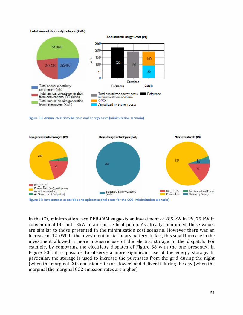
51

Figure 36: Annual electricity balance and energy costs (minimization scenario)

Figure 37: Investments capacities and upfront capital costs for the CO2 (minimization scenario)

In the CO2 minimization case DER-CAM suggests an investment of 285 kW in PV, 75 kW in conventional DG and 13kW in air source heat pump. As already mentioned, these values are similar to those presented in the minimization cost scenario. However there was an increase of 12 kWh in the investment in stationary battery. In fact, this small increase in the investment allowed a more intensive use of the electric storage in the dispatch. For example, by comparing the electricity dispatch of Figure 38 with the one presented in Figure 33 , it is possible to observe a more significant use of the energy storage. In particular, the storage is used to increase the purchases from the grid during the night (when the marginal CO2 emission rates are lower) and deliver it during the day (when the marginal the marginal CO2 emission rates are higher).

52

Figure 38: Electricity dispatch for the CO2 minimization scenario

5. Multi-objective optimization

As previously described, three reference runs must be performed prior to conducting multi-objective optimizations. These are the reference case, the cost minimization case and CO2 minimization case. Performing these runs allows setting the scaling factors for the cost and CO2 objectives, “MultiObjectiveMaxCosts” and “MultiObjectiveMaxCO2”. These values are obtained by finding the costs of a CO2 minimization run, and the CO2 emissions of a cost minimization run, respectively. In our case study we have already obtained all of the necessary information given the runs performed above, and for this reason we only need to update the scaling factors in the Parameters Table found in the Global Settings segment. Once this information has been introduced, we may now choose how each of the cost and CO2 objectives must be weighted, by setting the “MultiObjectiveWCosts” and “MultiObjectiveWCO2”, as shown in Figure 39 . These reflect the relative preference of the user over the criteria. Changing the goal to a multi-objective approach is done with the Options Table, by setting “MultiObjective” to 1.

53

Figure 39: Parameters table for multi-objective run

The button allows the user to choose some specific settings of the multi-objective

optimization. For example, it is possible to select the number of points to be included in the

Pareto frontier as well as the solver precision. Moreover, it is also possible to relax the

financial constraints of the problem, by letting cost and Payback period to increase, in

order to widen the limits of the multi-objective frontier. In our case study, we will allow a

10% increase of the costs in comparison with the base case (see Figure 40) so that lower

CO2 emissions solutions can be found.

Figure 41 presents the multi-objective frontier with 6 points. Besides the cost minimization

solution, it was possible to find 4 additional solutions with lower costs than the base case.

Due to the relaxation of the financial constraints, it was also possible to find 1 solution

leading to a significant decrease the CO2 emissions.

54

Figure 40: Multi-objective frontier options

Figure 41: Multi-objective frontier options

6. Cost minimization with existing technologies, forced investments and grid outages

In this section of the case study we assume that 100 kW of PV capacity are already installed

on-site although we are willing to consider additional PV. Additionally, we want to force

exactly 200 kWh of stationary battery capacity. Finally, in order to test the resilience of the

55

microgrid, we will simulate an outage from 5 pm to 8.30 pm during a weekday in

September.

First of all, because some equipment is pre-installed on-site, we need to run the base case

again taking the existing equipment into account. “DiscreteInvest” and “ContinuousInvest”

are set to 0 as in the initial reference case because no new investment is allowed, except

100 kW of PV that are now forced in the solution by setting “ForcedCapacity” to 100 and

defining it as “Existing”. Figure 42 shows the setting of the continuous technologies Forced

Investment Parameters.

Figure 42: Continuous technologies investment constraint

Also, outages costs need to be taken into account in this base case run. To model an outage three steps are required:

First of all, we set the number of emergency weekdays in September equal to 1 and decrease the amount of ‘normal’ weekdays from 20 to 19 (Figure 43).

Secondly, we set the hours during which the outage will occur: from 5 pm until 8.30

pm (Figure 44). This can be done in “Electric Utility Availability” table under Resiliency menu.

Finally, we chose to allow curtailment of electric loads by setting the maximum

hours of curtailment higher than 0 for all three priority levels and we assign a

variable cost to them. In this case we are not interested in heating load curtailments

and leave all the values of those parameters to zero.

It should be noted that the process of valuation of different load curtailments is a very

sensitive matter and will have a very significant impact on results. In order to properly

assess these numbers it is important to understand all costs that may incur due to loss of

56

load, including salaries of staff that may be sent home, costs of perishable goods, servers, or

any other relevant costs. While some tools may be already available to estimate these costs

(e.g. www.icecalculator.com), finding realistic values requires careful analysis and

understanding of the site being studied.

Figure 43: Number of days

Figure 44: Electric utility availability

Figure 45: Curtailment parameters

The total annual energy costs and total annual CO2 emissions for the base case are shown

on Figure 46 and will be used as reference for the investment runs. The base case cost is

57

now significantly higher due to the cost of curtailment, especially of mid and high priority

load. The electricity dispatch for the emergency weekday in September is shown on Figure

47. It can be seen that curtailment has occurred during the outage.

Figure 46: Results summary

Figure 47: Electricity dispatch for the base case with outage

After obtaining the new reference costs the investment run can be launched. We now allow new investments and set “ContinuousInvest” and “DiscreteInvest” to 1 in the Parameter Table found under Global Settings. In this case we have kept all technology options considered in the initial cost minimization run, but force a stationary battery of exactly 500 kWh. We also allow additional PV investment beyond the pre-existing 100 kW (Fig 41).

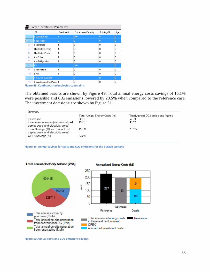
58

Figure 48: Continuous technologies constraints

The obtained results are shown by Figure 49. Total annual energy costs savings of 15.1% were possible and CO2 emissions lowered by 23.5% when compared to the reference case. The investment decisions are shown by Figure 51.

Figure 49: Annual savings for costs and CO2 emissions for the outage scenario

Figure 50:Annual costs and CO2 emissions savings

59

Figure 51: Investments capacities and upfront capital costs

No curtailment occurred as the new investments allow enough on-site generation to prevent them from happening (Figure 52).

Figure 52: Electricity dispatch with outage

It can be seen that during the outage period the loads are mainly served by the stationary

battery. Simultaneously, a significant part of the low priority load is curtailed. It should be

noted, however, that given the nature of the optimization algorithm, results are biased by

foresight. In other words, as every time steps is solved simultaneously and is equally

valued in the solution process, results reflect the anticipation of an outage, which will lead

60

to an optimistic use of the battery. Although this is a limitation of the current DER-CAM

version, it is possible to minimize this effect by applying the battery cycling obtained in

standard day-types to the end-use loads and re-adjusting the available battery size.

61

V. Case Study: multi-node version

In this section we will create a project and go through all the steps of the DER-CAM workflow to provide the user with some aspects of the multi-node version of the tool.

1. Starting the Project

As in the single node version, the multi-node project is started through the “New Project”

window. However, after naming the project and indicating the DER-CAM version, the user

should select the “multi-node” mode. This will disable the possibility of using the

embedded Load Databases in this window, since they can be used later to define the load in

each node of the microgrid. However, it is still possible to select Solar and Tariff data from

DER-CAM databases. To build our case, we will use the solar data regarding “San Francisco

International Airport” location and the “medium” utility tariffs in San Francisco, as shown

in Figure 53.

Figure 53: New project window (multi-node case study)

2. Power Flow and Heat Transfer Parameters

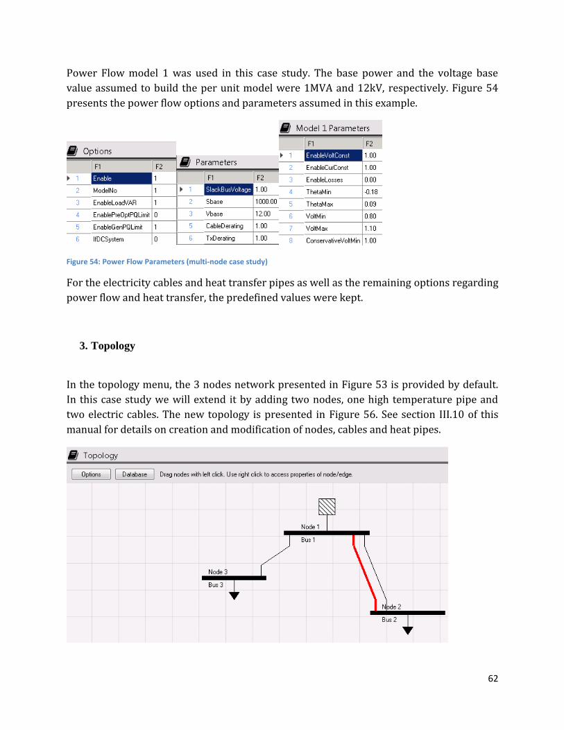
62

Power Flow model 1 was used in this case study. The base power and the voltage base

value assumed to build the per unit model were 1MVA and 12kV, respectively. Figure 54

presents the power flow options and parameters assumed in this example.

Figure 54: Power Flow Parameters (multi-node case study)

For the electricity cables and heat transfer pipes as well as the remaining options regarding

power flow and heat transfer, the predefined values were kept.

3. Topology

In the topology menu, the 3 nodes network presented in Figure 53 is provided by default.

In this case study we will extend it by adding two nodes, one high temperature pipe and

two electric cables. The new topology is presented in Figure 56. See section III.10 of this

manual for details on creation and modification of nodes, cables and heat pipes.

63

Figure 55: Default 3 node system.

Figure 56: Case study topology

In this instance, four electricity cables and two high temperature heat transfer pipes were

used to connect the nodes. The next table presents the characteristics of these connections

as well as their length. Cables and pipes with standard characteristics, provided in the

“Power Flow Parameters” menu, where chosen.

Connections Type Description Length

Node 1 Node 2 Electricity CU_XLPE_PVC_12KV_3CORE_25mm2 1200 Node 1 Node 3 Electricity CU_XLPE_PVC_12KV_3CORE_25mm2 1000

Node 2 Node 5 Electricity CU_XLPE_PVC_12KV_3CORE_25mm2 3000

Node 3 Node 4 Electricity CU_XLPE_PVC_12KV_3CORE_25mm2 3000 Node 1 Node 3 Heat HT Pipe Type 1 1000 Node 3 Node 4 Heat HT Pipe Type 1 3000

4. Load Database

The 5 nodes network topology comprises 4 consumption buses and a connection to the

electricity main grid. The following table summarizes the nodes characteristics and the

predefined databases used to build the load of each node. Details on how to use load

databases in DER-CAM multi-node version are provided in section III.5.2 of this manual.

64

Node Type Load Database

State City building Load Profile Ann Ele (scale)

Ann Gas (scale)

Node 1 PCC

Node 2 Load CA San Francisco Small Hotel New Const 5 5

Node 3 Load CA San Francisco Large Hotel New Const 8 8

Node 4 Load CA San Francisco Large Office New Const 8 8

Node 5 Load CA San Francisco Small Office New Const 6 6

5. Reference Scenario

As in the single-node version, a reference scenario is calculated prior to the definition of

the new investments. In this case study, the reference scenario does not include any

generation technologies, which means that the energy is purchased from the grid. However,

investments in conversion technologies (central heating and central cooling) should be

considered to supply the loads that cannot be directly supplied by electricity or gas. Thus,

Central HVACR investments were enabled in the Options Table of Global Settings. Also, a

high value of Base Case Cost should be defined in the Parameters Table ($100M). Figure 57

presents the Options and Parameters tables used for the Reference Scenario.

65

Figure 57: Options and Parameters tables in reference case (multi-node case study)

Figure 58 presents the summary results of the Reference Case. The total microgrids cost

(including annualized costs and electricity sales) is $10130K. The total energy was

purchased from the grid and investments in central heating and central cooling units were

made to supply heating and cooling loads from natural gas.

Figure 58: Summary Results of Reference Scenario (multi-node case study)

The “Topology” tab of the Results menu shows these investments per node. It is possible to

see in Figure 59 that central cooling units were included in all consumption nodes in order

to supply the cooling needs. However, only 3 of the 4 consumption nodes have central

heating capacity. This is due to the presence of the heating network – connecting the nodes

1, 2 and 3 – that allows the heating loads located at the node 2 to be supplied by the central

heating unit of the node 5, thus avoiding the fixed investment costs of an extra unit in node

2. In fact, by analyzing the heat dispatch in the node 5 (see Figure 60) it is possible to

observe that the heat generation is higher than the heat load consumption.

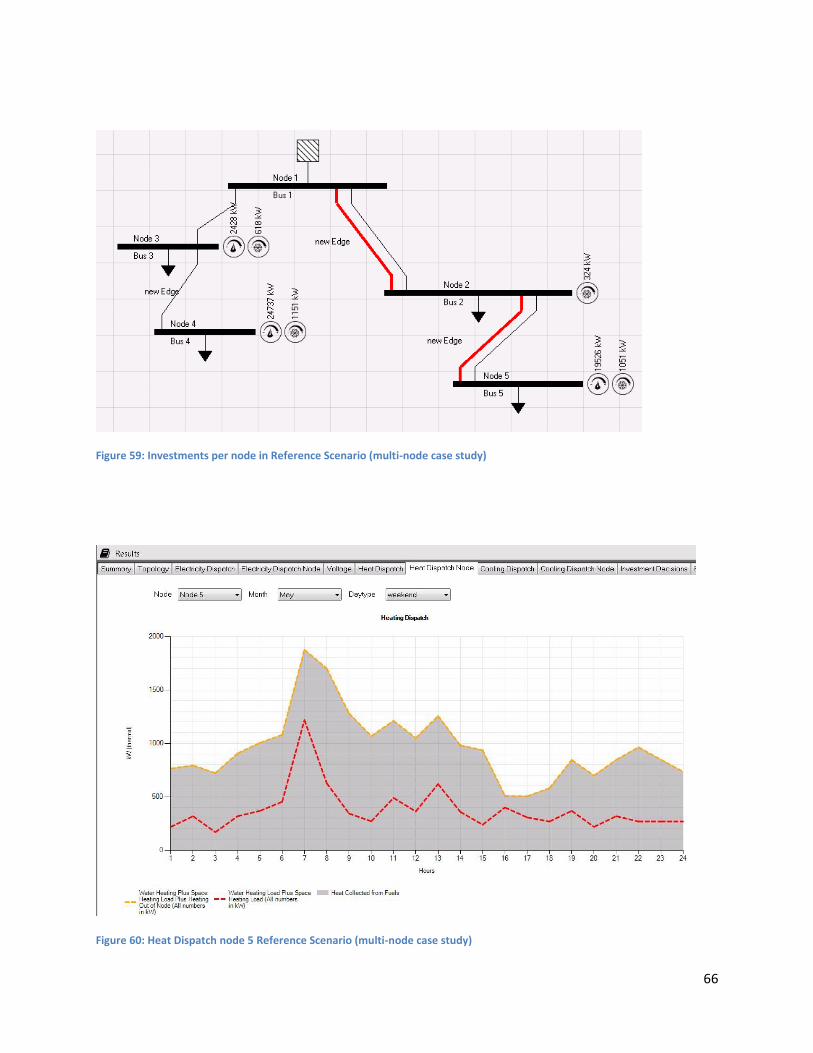
66

Figure 59: Investments per node in Reference Scenario (multi-node case study)

Figure 60: Heat Dispatch node 5 Reference Scenario (multi-node case study)

67

The “Detailed Results” tab of the results menu provides an exhaustive number of the

economic and technic values associated with the DER-CAM run. For example, regarding the

electric power flow, it is possible to obtain the maximum and minimum values of the

voltages deviations observed in each node, as shown in Figure 61.

Figure 61: Detailed Results (maximum and minimum voltages)

6. Investments Scenario

The scenario calculated in the previous section will be used as a reference for determining

new investments in the 5 nodes microgrid. Therefore it is necessary add the total cost of

the reference scenario before a new DER-CAM run. The exact value of this reference cost

can be obtained in the “Detailed Results” tab, as illustrated in Figure 62, and it should be

copied to the “Options Table” before a new run.

Figure 62: Total cost of the reference scenario

68

In order to allow DER-CAM to make investments in new DER assets it is necessary to select

the potential portfolio of technologies to be considered in each node. Besides the detailed

options regarding technical and economic aspects of discrete and continuous DER (see the

menu “Technologies” in section III.7), “Enable Investment” table should be used to specify

the types of investments per node. In this case study, we allowed investments in

continuous Technologies in all consumption nodes, as shown in Figure 63.

Figure 63: Enable Investments Table (multi-node version)

Figure 64 presents the summary results of the investment scenario. As shown in the figure,

the total savings in comparison to the base case scenario were 35%. This is caused by the

investments in photovoltaic generation in the microgrid (around 10 MW) that allow a

significant decrease of the operational costs. In fact, with these investments, the major

portion of the electricity needs are supplied by the PV capacity, while in the base case

scenario it was provided by the utility.

Besides the investments in PV panels, the optimal solution of DER-CAM also suggests that

part or the cooling loads should be supplied by absorption chillers, taking advantage of the

heat capacity during the summer periods. By looking at the investment per node in the

topology section of the results, it is possible to see that these new investments (PV and

absorption chillers) are located in the nodes 2 and 3.

69

Figure 64: Results Summary of the Investment Scenario (multi-node version)

Figure 65: Investments per node in Investment Scenario (multi-node version)

70

Figure 66 the impact of the new investments in the electricity dispatch of node 3 in June.

During the daylight periods, the PV capacity at the node is enough to supply all the loads of

connected this bus and to export to the node 4. Moreover, it is also visible the impact of the

absorption chiller, that uses heat to reduce the electricity cooling loads, represented in the

electricity dispatch as “Electric Cooling Load Offset”.

Figure 66: Electricity Dispatch per node - Investment Scenario (multi-node version)

The significant amount of PV generation in node 3 leads to an increase of the voltage in this

bus, especially around noon, as illustrated in Figure 67. However, these investments in

solar do not lead to any violation of the voltage limits specified in the power flow model.

71

Figure 67: Voltage per node - Investment Scenario (multi-node version)

72

Appendix A: Assessments Levels for DER-CAM use

1. Basic User Level

The Basic Level for DER-CAM is intended primarily for learning purposes or for quick

scanning of options at sites where the existing databases (energy loads, solar radiation, and

tariffs) are relevant.

This level requires users to pre-select a site by using the load, solar radiation, and tariff

databases present in DER-CAM. No entering of custom load, solar, and tariff data is

possible.

The menu options available are limited, and the available options are meant to help users

solidify the understanding of the workflow of DER-CAM models. As DER-CAM analyses

typically require both a reference run and an investment analysis run, these two run types

are available. However, run modifiers such as enabling power exports or forcing zero net

energy balance are disabled, and the technology options available are also limited and no

edits are allowed in any of the predefined technology parameters. This includes both

economic and performance data. The Basic User Level should enable fast and easy first

order microgrid assessment runs.

2. Intermediate User Level

The Intermediate DER-CAM user level includes all of the features available in the basic

mode, such as the loads, solar radiation, and tariff databases.

However, greater flexibility and a wider number of features is made available to the user as

all of the database inputs (loads, solar radiation, and tariffs) may be customized by users to

model more complex situations. Furthermore, the Intermediate User Level allows using of

some of the Load Management and Resiliency features, including the definition of outages

and load priority levels for load curtailment analysis in islanding conditions. It is equally

possible to enable power exports of onsite generation, as well as the definition of feed-in

tariffs and power export conditions (minimum and/or maximum requirements).

The Intermediate User Level does not allow changing technology parameters, but enables

users to test microgrid conditions including outages (forced islanding) and gauging the

tradeoff between outage costs induced by load curtailments and investment costs from

additional DERs to serve loads when the utility is unavailable.

73

3. Advanced User Level

The Advanced DER-CAM user level includes all of the features available in the Intermediate

User Level, including the ability to edit energy loads, solar radiation data, as well as tariff

information.

In addition, all technology definitions are now unlocked and users are allowed to modify

existing data and input custom technologies. Additional load management features are

enabled, including load shifting and demand response.

By enabling these features users can not only define real sites, but also express the

technical characteristics of DER equipment relevant to a particular manufacturer, rather

than using the reference values made available through the DER-CAM template.

The Advanced User Level empowers users with all of the most commonly used DER-CAM

features, and will typically allow building a customized microgrid model that fully covers

the case under study.

4. Full User Level

The Full User Level of DER-CAM grants users complete access to all input data and

parameters that are required to build the most complex models. Energy loads, weather

data, tariff information, technology options, and energy management options are all

enabled, thus allowing very complex models to be created.

All features available in the Advanced User Level are included in the Full User Level, and

additional features are now enabled, namely building shell improvement measures,

financial incentives such as investment subsidies and performance based incentives, net

metering, and Zero Net Energy constrains. This level requires advanced experience and

training in using DER-CAM.

74

Figure 1: Start Window ................................................................................................................................. 8

Figure 2: New Project Window ................................................................................................................... 10

Figure 3: Information on Load Data window .............................................................................................. 12

Figure 4: Information on Solar Data window .............................................................................................. 12

Figure 5: Information on Tariff data ........................................................................................................... 13

Figure 6: Input Main Screen ........................................................................................................................ 14

Figure 7: An example for solar insolation data ........................................................................................... 21

Figure 8: Access to load database in multi-node version ........................................................................... 23

Figure 9: Topology....................................................................................................................................... 33

Figure 10: Nodes proprieties and new edges ............................................................................................. 33

Figure 11: Nodes proprieties and new edges ............................................................................................. 34

Figure 12: Line parameters ......................................................................................................................... 35

Figure 13: Creation of a new project .......................................................................................................... 36

Figure 14: Option and Parameter Table ..................................................................................................... 37

Figure 15: Number of days Table ................................................................................................................ 38

Figure 16: "Site Weather Settings" Tables .................................................................................................. 39

Figure 17: Wind Power Potential ................................................................................................................ 39

Figure 18: Loads Table ................................................................................................................................ 40

Figure 19: Tariff tables in DER-CAM ............................................................................................................ 41

Figure 20: Fuel Price table........................................................................................................................... 41

Figure 21: CO2 emissions tables in DER-CAM ............................................................................................. 42

Figure 22: Result View, Summary Sheet ..................................................................................................... 42

Figure 23: Results View, Detailed Results Sheet ......................................................................................... 43

Figure 24: Parameter and Option Table ..................................................................................................... 44

Figure 25: Generation Constraints .............................................................................................................. 45

Figure 26: DER Technologies Info ............................................................................................................... 46

Figure 27: Forced Investment parameters for continuous technologies ................................................... 46

Figure 28: Investment Parameters for continuous technologies ............................................................... 47

Figure 29: Investment summary section in the result sheet ...................................................................... 48

Figure 30: Annual Savings of energy costs and CO2 emissions .................................................................. 48

Figure 31: Annual electricity balance and energy costs.............................................................................. 48

Figure 32: Investments capacities and upfront capital costs ...................................................................... 49

Figure 33: Electricity Dispatch ..................................................................................................................... 49

Figure 34: Options Table ............................................................................................................................. 50

Figure 35: Annual savings for costs and CO2 emissions for the CO2 (minimization scenario) ................... 50

Figure 36: Annual electricity balance and energy costs (minimization scenario) ....................................... 51

Figure 37: Investments capacities and upfront capital costs for the CO2 (minimization scenario) ........... 51

Figure 38: Electricity dispatch for the CO2 minimization scenario ............................................................. 52

Figure 39: Parameters table for multi-objective run .................................................................................. 53

Figure 40: Multi-objective frontier options ................................................................................................ 54

Figure 41: Multi-objective frontier options ................................................................................................ 54

Figure 42: Continuous technologies investment constraint ....................................................................... 55

75

Figure 43: Number of days .......................................................................................................................... 56

Figure 44: Electric utility availability ........................................................................................................... 56

Figure 45: Curtailment parameters............................................................................................................. 56

Figure 46: Results summary ........................................................................................................................ 57

Figure 47: Electricity dispatch for the base case with outage .................................................................... 57

Figure 48: Continuous technologies constraints ........................................................................................ 58

Figure 49: Annual savings for costs and CO2 emissions for the outage scenario ....................................... 58

Figure 50:Annual costs and CO2 emissions savings .................................................................................... 58

Figure 51: Investments capacities and upfront capital costs ...................................................................... 59

Figure 52: Electricity dispatch with outage ................................................................................................. 59

Figure 53: New project window (multi-node case study) ........................................................................... 61

Figure 54: Power Flow Parameters (multi-node case study) ...................................................................... 62

Figure 55: Default 3 node system. .............................................................................................................. 63

Figure 56: Case study topology ................................................................................................................... 63

Figure 57: Options and Parameters tables in reference case (multi-node case study) .............................. 65

Figure 58: Summary Results of Reference Scenario (multi-node case study) ............................................ 65

Figure 59: Investments per node in Reference Scenario (multi-node case study) ..................................... 66

Figure 60: Heat Dispatch node 5 Reference Scenario (multi-node case study) ......................................... 66

Figure 61: Detailed Results (maximum and minimum voltages) ................................................................ 67

Figure 62: Total cost of the reference scenario .......................................................................................... 67

Figure 63: Enable Investments Table (multi-node version) ........................................................................ 68

Figure 64: Results Summary of the Investment Scenario (multi-node version) ......................................... 69

Figure 65: Investments per node in Investment Scenario (multi-node version) ........................................ 69

Figure 66: Electricity Dispatch per node - Investment Scenario (multi-node version) ............................... 70

Figure 67: Voltage per node - Investment Scenario (multi-node version) ................................................. 71

DER-CAM User Manual - Building Microgrid full... · 5 I. Introduction to DER-CAM Web Optimization...

Documents

Transcript of DER-CAM User Manual - Building Microgrid full... · 5 I. Introduction to DER-CAM Web Optimization...