Understanding, Deploying and Configuring the User Profile Service

1
Deploying, analysing and configuring wireless sensor networks
Written by: Joris Ahsmann
Date: 1 July 2013
Student at: Technische Universiteit Eindhoven(TUe)
Tutor TU/e: Twan Basten
Location: Cork Institute of Technology
Department : Nimbus Centre
Tutor CIT: Alan McGibney

2
Table of contents Table of contents.................................................................................................................................... 2
1 Preface ........................................................................................................................................... 3
2 Introduction ................................................................................................................................... 4
General ................................................................................................................................... 4 2.1
Research Goals ....................................................................................................................... 4 2.2
Thesis Outline: ........................................................................................................................ 5 2.3
3 Current State of Research in Wireless Sensor Networks ................................................................ 6
Wireless Sensor Network Architecture ................................................................................... 6 3.1
The Routing ............................................................................................................................ 8 3.2
The planning ......................................................................................................................... 11 3.3
Quality of Service Support .................................................................................................... 12 3.4
Nimbus Wireless Sensor Network Test-bed ......................................................................... 13 3.5
The wireless deployment tool .............................................................................................. 17 3.6
Conclusion ............................................................................................................................ 19 3.7
4 How to analyse and configure a wireless sensor network ............................................................ 20
Analysing a network ............................................................................................................. 20 4.1
Configuring the network ....................................................................................................... 30 4.2
Determining the required configuration .............................................................................. 37 4.3
Verification of the analysis and configurations on real deployment’s .................................. 42 4.4
The analysis tool ................................................................................................................... 51 4.5
Conclusion ............................................................................................................................ 57 4.6
5 Linking the Deployment to the Design ......................................................................................... 59
The multi wall model: ........................................................................................................... 59 5.1
The ray tracing model ........................................................................................................... 61 5.2
Analysis based on site survey data ....................................................................................... 63 5.3
Ray tracing model adjustment based on the data from real deployments........................... 68 5.4
Conclusion ............................................................................................................................ 71 5.5
6 Conclusion .................................................................................................................................... 74
7 Bibliography ................................................................................................................................. 77

3
1 Preface This thesis marks the end of my study Embedded Systems at the Techinische Universiteit Eindhoven.
For the last nine months I’ve been welcomed by the nimbus Centre which is part of the Cork Institute
of technology to conduct my research for this thesis. I have found Nimbus a pleasant place to work
thanks to all the people who work here.
During these 9 months I´ve been doing research regarding the behaviour of wireless sensor network.
In this research I had the opportunity to use a within Nimbus developed test bed. This gave me
opportunity to analyse the behaviour based on a real deployment. For which I want to thank Davide
Pusceddu, who has been helping me understanding the test bed during these nine months. Next to
that I would like to thank Alan McGibney, who has my supervisor and the one who gave me guidance
and was always willing to help me out in case of issues.
At the end I would like to give special thanks to Twan Basten, who was always available for feedback
and commends on my work. I found the feedback I got from him very detailed and clear and helped
me a lot during this period.
Joris Ahsmann

4
2 Introduction
General 2.1Advances in modern day technology have enabled engineers to develop small, low cost wireless
sensor devices that can communicate with each other and form large networks of sensing and/or
actuating devices. These networks are now being used to obtain dense environmental data for
applications such as habitat monitoring [1], flood warning [2] or fire detection in for example forests
[3] or tunnels and provide engineers the ability to move from beyond basic centralized sensing and
controlling of the environment to large scale sensing and distributed control systems.
The development of wireless sensor networks (WSN) has many different aspects to be considered
such as sensor calibration, data reliability and power management. As the scale of deployments has
increased significantly in recent years one of the key focal points of research has been the challenges
related to the deployment and configuration of WSN. A WSN typically consists of small, low cost,
wireless battery powered nodes. The objective is to deploy the nodes in such a way that the network
matches the required sensing criteria, maintaining a reliable communications link and maximising the
lifetime of the network all at minimal cost. To achieve all these goals is a non-trivial task even for the
experienced designer.
Research Goals 2.2WSN are deployed for many different environments and purposes all having their own challenges.
Due to the dynamic nature of buildings and the complexity of radio propagation within them they
pose a significant challenge when it comes to planning and design of wireless applications. The
biggest challenge associated with these networks is ensuring reliable connectivity between the nodes
while maintaining a reasonable lifetime. Walls, furniture and people all influence how a wireless
signal propagates through the building and this can have an adverse effect on network performance.
Even if the influence of a building is taken into account at design time, the dynamic nature of a
building can often lead to unpredictable behaviour of the WSN during its lifetime. Once a sensor
network is deployed and operating it generally collects all the sensed data at a centralized point for
processing within business applications. Analysing how data travels through the network and
ensuring it operates as expected can be a difficult task due to the large amount of data and dynamics
of the network behaviour.
The research presented in this thesis will focus on the development of tools and methodologies to
analyse and configure WSN in buildings and it investigates how these tools and the information
gleaned from them can be used to improve the quality of a site specific deployment. More
specifically the research will investigate the following:
1. What data can be extracted from a live network and how can it be used to analyse and verify
the performance of the WSN post-deployment
2. How can the network be configured/re-configured to ensure requirements are met while
maintaining a maximum lifetime
3. How can the extracted information/QoS metrics be feed back to the design phase to improve
on the site specific deployment.

5
Thesis Outline: 2.3Frist Section 3 will focus on the state of the art in wireless sensor networks, the focus will be on the
components in wireless sensor networks, routing protocols and quality of service provisioning. After
this the test bed is analysed. What components are used and what is implemented in this test bed.
Section 3.5 will present the analysis of the WSN test bed. This includes a description of the different
components as nodes, routing protocol and the deployment tool.
Section 4 will identify what metrics will the test bed produce for analysis and how do those metrics
reflect he quality of the network. Once the analyses of the network can be made the information is
used for quality of service provisioning is presented. This research resulted in the development of an
analysis tool, and analysis descriptions for the physical, link and transport layers in the network. Next
to that a QoS provisioning method is introduced. This tool is used to visualize the status of the
network and all the data it produces.
Section 5 will focus on how real time information from the network can be feed back to the design
step and potentially be used to identify issues within the network and ultimately improve the quality
of the initial design.

6
3 Current State of Research in Wireless Sensor Networks Research in WSN started in the US military. One of the first WSN was developed by the American
army in the sixties which was used to detect Soviet submarines [4]. The network consisted of
submerged acoustic sensors which were deployed over the pacific and Atlantic oceans. For a long
time WSN has only been a subject for military use and research. This is mainly due to its cost.
However recent advances in technology made wireless systems cheaper and more energy efficient.
This drove the proliferation of WSN as they became affordable for commercial use, which intensified
the research and applications of wireless sensor networks.
When using WSN different challenges have to be faced. All of those challenges are related to the
resource constraints on the sensor nodes. Since all nodes are wireless they should have all resources,
such as power, memory, computational power and communication capabilities on board. Therefore
the first challenge is the selection of which nodes should be used for the application; what should a
node be capable of; how should those nodes communicate; and how long should they last without
changing or recharging the batteries. After the choice of nodes is made the next challenge is how to
create a network. How should the nodes route their data through the network to form a fully
connected network. This is strongly related to the challenge of deployment planning in WSN. This
involves addressing how to position the nodes in such a way that they are able to form a network
which is able to fulfil its task. Once the network is deployed the next challenge is how to configure
the network in such a way that is meets its requirements which are given by the quality of service
(QoS).
The topics of interest are listed here and the current state of the research will be discussed in this
section.
- The wireless sensor network architecture
- Routing packets through the network
- Planning of the network
- Quality of Service support
On the first three points, the network architecture, routing and planning of the network, research is
more or less crystallized. The general picture is clear and different types are defined. However the
quality of service support for wireless sensor network is still an open ended research topic. Several
research works have been published over the last few years but they all focus on their own specific
types of quality of service. I couldn’t find a common notion on the definition of quality of service for
WSN and assumes that still does not exist yet.
Wireless Sensor Network Architecture 3.1A wireless sensor network typically consists of three types of components, sensor nodes, sinks and
relay nodes. The sensor nodes are responsible for the sensing and actuation. Relay nodes can be
added as an intermediate to create a fully connected network if sensor nodes are unable to reach the
sink. A sink collects all the data from the sensor nodes for centralized processing and/or storage. This
is illustrated in Figure 1

7
Sensor node
Sensor node
Sensor node
Physical worldWireless network
Relay nodes
Sink
Sink
Figure 1: Wireless Sensor Network Architecture
Typically radio signals are used to connect the nodes with each other. Commonly used radio
communication protocols for low power networks are ZigBee [5], WirelessHART [6], 6LowPAN [7].
These protocols work on the 2.4GHz band and are all based on the 802.15.4 standard, a standard for
low power wireless communication. The most wireless sensor networks used today are based on one
of those protocols however all industrial, scientific and medical bands (ISM) can be used for
communication. The frequencies of those bands are
Industrial, scientific and medical bands
6765–6795 kHz
26,957–27,283 kHz
40.66–40.70 MHz
433.05–434.79 MHz
902–928 MHz
2400–2500 MHz
5725–5875 MHz
24–24.25 GHz
61–61.5 GHz
122–123 GHz
244–246 GHz
On top of the physical connectivity the wireless sensor network often inherits a basic version of the
IPv6 protocol stack such as 6LowPAN. Using the IPv6 stack makes the integration of the system with
the internet straight forward and also makes the support which can be used for the IPv6 stack
available for maintaining the network.
Nodes 3.1.1
A node is the component that captures sensed data from the environment and sends this data to a
sink and typically consists of the following four components:
- Sensor(s)
- Controller
- Communication device
- Battery
The sensors are form the connections between the physical world and the wireless sensor network.
All different sized sensors exist, for example temperature, light or humidity sensors. The controller is

8
the heart of the node; this normally is a small controller that is used to perform aggregation on the
data and controls the sensors and the communication of the node. The communication device is the
antenna for the communication often combined with a controller that is used to control the antenna.
And the battery is the energy source of the node. This could vary from some small to large batteries.
This depends on the required lifetime and application of the network.
Sensors can operate in three modes. The first mode is that the sensor periodically sends its sensor
data to a sink where it will be processed; this is called periodic sensing. The second mode is event-
based where the sensor is programmed only to send data when a certain event occurs, for example,
when a sensor reading exceeds a pre-defined threshold value. And the third option is a query mode.
In this mode a sensor will not send data out of its own but will only respond to query’s send to it
from other nodes or applications.
The node lifetime is mainly determined by the activity of the radio chip and the battery. To increase
the lifetime the radio chip is periodically turned on to see if other nodes want to send data to it, or to
transmit its own packets. This is done is a synchronized manner so that when a node transmits a
packet the other nodes are able to listen. If there is no more communication on the link all nodes
turn of their radio chip and turn on again in the next period. In [8] this mechanism known as the
nodes duty cycle is described. The duty cycle and can have a great influence on the latency and
energy consumption of the packets and nodes.
Sinks 3.1.2
The purpose of a sink is to collect sensor data and process it or send it to another location where it
will be processed and/or stored. What it does with the data depends on the application which
requires the data.
Due to the computational demand a sink is normally connected to a power source and therefore has
no or less power constraints than a node. With this in mind, in many cases the sink can not only be
responsible for the gathering of the data but also for maintaining and organizing the sensor network
topology. The routes that the sensors should use can be determined at the sink as it has the
capability to analyse the network status and create routing tables based on the observed network
activity. This is however only done for relatively small networks, otherwise the induced overhead on
the network to send all data to the sink required to create the routes is too large. In these cases it is
better to locally determine the routes .
Relay nodes 3.1.3
A sensor should be placed at the location where it can sense the highest quality of data. Due to walls,
furniture, people and the size of the building sensors could be too far apart for a single sink to be
placed within range of all of the sensors. To solve this mesh routing can be used. When a network
gets fragmented, extra communication nodes can be deployed to cover the entire area; these nodes
are called relay nodes.
The Routing 3.2The quality of the network is highly related to the routes the network uses. Typically the network is
able to select different routes to route the data through the network. The routing protocol is
responsible for selecting the routes in the network and determining the routes in the networks
involves selecting for each node to which other node it should send its data. In a mesh networks

9
forming the routes in such a way that all nodes are connected can be a hard task. Many different
options exist and finding the optimal topology can be difficult.
WSN are used for many different purposes and can be in various sizes, each purpose and size will
have its own characteristics and requirements, and can have all other ways to route data through the
network. When routing data through a network, different quality metrics for the used topology
exists. A topology should in the first place be able to let all the nodes in the network route their data
through the network to, in the case of WSN, a sink. Next to this several optimization goals can be
distinguished. The main options are lifetime optimization, redundancy, latency minimization and
reliability optimization [9].
Lifetime optimization involves creating a topology in which the lifetime of the network is optimized.
Usually the lifetime of the network is defined as the lifetime of the node with the shortest lifetime. In
order to optimize the lifetime of the network the topology should be balanced. This means that the
load on all nodes should be as equal as possible. A completely balanced network is however
infeasible [1]. All nodes will send their data back to a sink, when they cannot reach the sink directly
multi-hop routing is used. This results in the nodes closer the sink always having a higher load than
nodes on the edge of the network. Lifetime optimized routing protocols try to balance the load as
much as possible while maintaining a network in which all nodes are connected.
Redundant routing is an approach used to optimise the reliability of the network. This type of routing
involves sending the data over multiple links. This way when the data packet is dropped on one link,
the other path might still succeed which causes probability that data is lost is reduced. The challenge
in this type of routing is how to ensure multiple paths for all nodes which are also reliable and have a
minimal impact on the network.
Latency minimisation routing tries to minimise the maximum latency of all nodes. The simplest
example of latency aware routing is to minimize the number of hops. But also more complex latency
aware routing protocols exists that includes for example the duty cycle of the nodes.
The last routing optimisation option is the reliability. This involves optimising the reliability of the
path from a node to the sink. The reliability can be measured as the probability that a packet is
successfully propagated through the network. Therefore when creating a network topology, the links
over which the packets are routed, should be as good as possible. Those quality metrics should be
used when creating a topology. Creating a topology can be done several different ways. The most
common ones are listed here.
- Static routing
- Centralized routing
- Decentralized routing
Those 3 listed types will be discussed in this section.
Static Routing 3.2.1
Static routing means that all routes in the network will be determined pre-deployment. No online
analysis of the network is done. This type of routing is common in small networks where the
environment is static. An example of a commonly used static routing method is the star topology as
in Figure 2.

10
Sensor node
Sink
Sensor node
Sensor node
Sensor node
Sensor node
Sensor node
Figure 2: Star Topology
All nodes will send their data directly to the sink, and must therefore be in the communications range
of the sink. Larger, multi hop static routing is also possible and normally only used in small networks
because all routes have to be determined by hand pre-deployment.
Centralised routing 3.2.2
Centralised routing means that on a central point, normally the sink the routes in the network are
determined. All nodes will check which nodes are within its communication range, and what the
qualities of the links are. This data is than sent to the sink which than determines which link the
nodes should use to send its data.
The advantage of using centralised routing is that the routes of the nodes do not have to be pre-
determined. Also the network is able to respond to changes in the network. Normally the nodes will
periodically send status updates to the sink. Based on those status updates the sink can decide to
change the used topology. This way the network is able to respond to changes in the network.
The advantage of doing this in a centralised way is that at the central point an overview of the
complete network is available. Thus when creating a topology the impact on each node can be
considered and a global optimum can be determined. However the downside of creating a network
in a centralised way is that all nodes will have to send status updates to a centralized point. For small
networks this not a problem. However WSN could scale up to thousands of sensors. In these
situations created extra load might overload the network, reducing its lifetime and consuming the
available bandwidth.
Decentralised Routing 3.2.3
When using decentralised routing nodes or groups of nodes, will define their routes based on local
knowledge. Using decentralised routing will give nodes the ability to independently define their
routes using the information of their neighbours. The required information to select a route depends
on what type of routing is used. Different routing protocols will rely on different types of metrics to
form its route decision.
The major advantage of this method is that nodes are able to locally define their own route which
means that the network is able to maintain its own topology without the need of a central node or
sink to gather all the data and define the routes. The disadvantage of this approach is that there is no
global knowledge of the topology this might lead to inefficient topologies which from local

11
perspective is the best possible. Also this method can create a higher computational load on the
nodes. For large networks this type of routing is preferred since the added load on the nodes
resources is a static load for each node whereas when using the centralized routing the load on the
nodes increases by the size of network.
The planning 3.3A WSN has two major functions, sensing and communicating. When deploying a WSN, those two
functions are the most important things to consider in order to ensure a network is capable of
meeting application requirements. Next to these functions there is also a set of secondary
requirements. The secondary requirements focus more on the quality of the deployed network. Both
are discussed in this section.
Primary requirements 3.3.1
3.3.1.1 Coverage
Each sensor type has different constraints for covering an area. For example, one temperature
sensor could be sufficient to cover a room, where maybe multiple sensors per room are required to
sense movements. The properties of all sensors should be used to create a network which covers all
the requirements of the sensor network. Coverage involves the placement of sensors in such a way
that all the required sensing data for the application can be sensed. To design a sensor network
which has full coverage with the minimum number of sensors is often optimally solvable in 2D but
becomes NP-Hard in 3D [10]. NP stands for non-deterministically polynomial and implies that
typically no optimal solution can be computed based on the current computing power and algorithm
knowledge within reasonable time. Therefore most application designers create a 2D abstraction of
their environment instead of using a 3D version.
3.3.1.2 Connectivity
The connectivity problem involves making sure that all nodes are able to send their data to a
centralised point, normally the sink. When the coverage problem is solved in a 2 dimensional
abstraction, a set of sensing nodes are placed on a 2 dimensional plane. Those nodes should than try
to form a network and often the sensor nodes alone form a fragmented network. Therefore relay
nodes should be added. Since adding relay nodes involves an increase of the price, the number of
added relay nodes should be kept to a minimum. In [11] a Steiner Minimum tree with minimum
number of Steiner points and bounded edge length (SMT-MSP) is used to solve this problem, and this
problem is proven to be NP-Hard. Therefore computing the optimal solution is not tractable and
other non-optimal solutions will have to be used.
Secondary requirements 3.3.2
Along with the primary requirements connectivity and coverage, there is also a set of secondary
requirements. Those requirements are used to cover the price and quality of the network and should
be considered when creating a deployment. The requirements are:
- Lifetime
- Throughput
- Latency
- Cost

12
3.3.2.1 Lifetime
Lifetime involves the duration of the network that it is capable of operating. Since sensors and relay
nodes are battery powered their lifetime strongly depends on the amount of energy required for
operation. When the network is designed with a minimum number of sensor and relay nodes the
death of a single node could cause all nodes relying on that node to become disconnected. Therefore
the system should try to balance the power consumption of all nodes in the network in order to
maximize the lifetime. Balancing the power consumption involves minimizing the distance between
nodes to be able to reduce the transmission power. This is because communication is a key energy
consumer as the radio signal power in the network drops off with d4, where d is the distance
between the transmitter and the receiver [11]. When balancing the distance between nodes the
energy consumption per transmitted packet is balanced, however a wireless sensor network often is
a multi-hop network. So also the number of packets a node needs to send should be balanced. When
there is a single node forwarding the data of multiple nodes, its battery will deplete much faster
resulting in a shorter lifetime of the network. Due to this multi hop property of a mesh topology the
nodes close to the sink will deplete their batteries quicker than nodes at the borders of the network.
This problem can sometimes be reduced by actively measuring the remaining lifetime of the nodes
and to spare the nodes with the lowest lifetime.
3.3.2.2 Throughput
Throughput involves the amount of data a node can transmit per time unit. When the network scales
up, the amount of data it produces increases. Because of the multi-hop property the nodes close to
the sink will have to forward more data when the size of the network increases. When the network is
designed it should be made sure that no nodes are overloaded. Thus it should be assured that the
bandwidth is sufficient for all nodes’ demands. When determining the throughput it is important to
consider that it is impossible for multiple nodes that are within range of each other to transmit data
at the same time since then their signals will interfere with each other. Thus when checking whether
the bandwidth is sufficient the load of the nodes within range of each other should be combined.
3.3.2.3 Latency
Latency involves the time it takes to transmit a packet from a node to the sink. When the application
contains latency constraints the network should be able to meet these constraints. The latency is
strongly related to the number of hops a packet takes from a node to the sink. When this number is
too large, the distance between the nodes should be increased to lower the number of required hops
from the node to the sink. This requirement is fully dependent on the application requesting the
data.
3.3.2.4 Cost
Cost involves the price of the network as a whole, as each node (sensor, relay, sink) will cost money,
the number of nodes required for the network should be kept to the minimum. The optimisation goal
for cost can be described as follows. Given the requirements of the sensing network, create a
network with the minimum number of nodes while satisfying the requirements.
Quality of Service Support 3.4Defining quality of service (QoS) is always an important aspect in designing a system. The QoS defines
requirements for the system and heavily relies on the applications using the system. Based on those
requirements the system should determine how it utilises its resources. QoS frameworks for
13
traditional networks have existed already for years; however WSN are different from traditional
networks due to the strict resource constraints on the nodes. That difference also requires different
methods to define the required QoS. A new extended QoS definition method will have to be applied
on WSN. In [12] a survey is given on what options there are to specify QoS requirements for WSN.
This survey shows that due to the wide variety it is hard to create one basic QoS framework.
Currently QoS support for wireless sensor networks is one of the open research topics. Different
models for different types of QoS are developed, but there is not yet a common notion of how to
handle QoS support in WSN. This also depends on the application; currently different QoS support
frameworks are developed to support different types of application.
What the most QoS support methods have in common is that the required quality of service is
specified in two layers. The Application specific layer and network specific layer [13].The application
QoS requirements will specify the application needs in terms of for example coverage or sensor
accuracy. The network related QoS involves the metrics which are often known from traditional
networks. Metrics as throughput, latency, lifetime and reliability are the most important ones and
are often derived based on the application QoS.
The challenge when creating a QoS aware WSN is that the metrics used are often conflicting, for
example reliability and lifetime. In [14] a method is introduced that tries to optimise the lifetime of
the network by periodically turning redundant nodes off, and use energy aware routing protocols.
This comes at the cost of a lower reliability of the network. However this cost is kept to a minimum
by measuring the remaining quality and when this becomes too low the nodes will not be turned off
or other routes are used.
Nimbus Wireless Sensor Network Test-bed 3.5The QoS methodology and experiments presented in this thesis will utilise the Nimbus WSN test bed;
in this section the components of the test bed is introduced. Firstly all network components, nodes,
sink and used data packets will be described. After this the developed wireless sensor network
deployment tool is introduced.
The network components 3.5.1
The Nimbus WSN is composed of the TelosB sensing platform developed by Crossbow [15]. These
devices are deployed with the open source TinyOS operating system. For the sink a mini computer is
used. And the network itself is a periodic-based sensing network. All components used in the test
bed, and the communication protocols are discussed in the following subsection.
3.5.1.1 Sensor Nodes
The TelosB node has IEE802.15.4 communication capabilities with an on-board antenna and contains
a “TI MSP430” microcontroller and a set of on board sensors including light, temperature, humidity
and supply voltage sensors. The power supply of those nodes consists out of two AA batteries. The
node is shown in Figure 3.
.

14
Figure 4 - TelosB Sensor Node [15]
In the test bed sensor nodes periodically send two types of packets, sensor packets and statistics
packets. The sensor packets contain information about the sensor readings whereas the statistics
packet contains information about the behaviour of the sensor for example the address of its parent
and the quality of the used link. The periods of the packets is configurable and can vary from once
per couple of seconds to once per hour. The used period will be determined by the application
requesting the data.
3.5.1.2 The sink
The sink consists of a node, just like all the others, combined with an embedded PC connected to the
LAN and running a stripped version of Linux. The node will be used to receive the data from the
WSN, and the computer to execute all the sink tasks. The responsibility of the sink is to send all the
received data to the next layer in the system. This can either be a database or an application.
Figure 5 A sink
As well as sending the data from the nodes to an application, a sink can also be used to debug the
network, and reconfigure the nodes. The sink will be informed by the nodes about their status and
routes; In the Nimbus test bed nodes send status reports regarding their links and topology back to
the sink. Since indoors the networks or node clusters do not tend to be as large as for example forest
fire detection and can therefore handle this extra load. This information can be used to debug and
analyse the network. In terms of reconfiguration the sink can be used for example to change the
sensing period or the communication channel being used.
3.5.1.3 The Application Layer
The application layer has as input the data from a sink; this can be either a single sink or multiple
sinks. At the moment this layer will parse the packets and store the data in a database for later use.
The middleware layer could also be used to develop and execute applications which rely on the data
from the WSN. For the purpose of this document, storing the data can be seen as the application.
The relationships between all components are illustrated in Figure 6:

15
Sensor
Sensor
Sensor
Sensor
Sensor
Network
Sink
Sink
Application layer
DB
Figure 6: Full system
3.5.1.4 Hydro Routing Protocol
Since the routing protocol has a great influence on the behaviour of the routing proctor does this
from an crucial element for the network. In the test-bed a routing protocol called Hydro is used.
Hydro [16] is a decentralized routing protocol used by the WSN to determine the routes in the
network. This means that each node itself determines which node it chooses as its parent. Nodes
periodically send data to each other that summarises the status of their connection to the sink. The
ETX metric is used for this. ETX stands for the estimated number of transmission to successfully
transmit a packet and is a link quality indicator.
If a node A connects to the sink it will actively measure its ETX value to the sink. When another node
B asks what the status of that node’s connection is it will send the ETX value to the other node. Node
B could receive ETX values of multiple nodes; in that case it will try to connect to one with the lowest
value.
Node B will also measure the ETX value of the link between itself and its parent. But now when a
node asks for the status of its link it will add its own ETX value to the value of its parent and send that
to nodes asking for it. In this way, the ETX values cumulatively add up, and when the number of links
to be traversed to the sink becomes larger the ETX values will also be larger. This is because the
smallest ETX value is 1.
A node will always try to connect to the node which has the lowest ETX value. In that way, a node
tries to use the least amount of links, and tries to connect to the strong links, since the weak links will
have a higher ETX value. However this works for relatively small networks. For example when a rout
from a node contains 10 hops and all the nodes will have an ETX of 1.1 the cumulative value will be
11, which equals a route containing 11 hops with an ETX value of 1. In such a case the routing
protocol is unable to distinguish the quality of the route with its length. The simplicity of this protocol

16
allows nodes do determine their own routes, however since there is no global notion of the network
those routes might not lead the optimal routes of the network.
3.5.1.5 Nimbus WSN Packet Types
In the Nimbus WSN, two types of packets are used, Sensor packets and Statistics packets. The Sensor
packets give information about the readings of the sensors and contain some additional information
about the status of the links. The status of the links is measured by the radio chip on the node. This
radio chip measures the received signal strength indicator (RSSI), and the link quality indicator (LQI),
values of incoming signals. A link will be measured two ways, from the node to its parent, the route
which the sensor data will take and thus the most important one for the application point of view
and from the parent to the node. Since data flows both directions the link can also be measured both
directions.
Next to the link status the nodes also keep counters to be able to monitor the different activities of
the nodes. Those counters involve the number of forwarded packets, number of packets inserted in
the network, number of routing protocol messages to name a few.
The following lists show the different data fields in the different packets.
The sensor packets:
Temperature
Humidity
Supply voltage of the node
Light intensity
The worst measured RSSI on the link between the parent and the node in the last sensing period
The worst measured LQI on the link between the parent and the node in the last sensing period
Address of the parent
The worst measured RSSI of all connected children in the last sensing period
The worst LQI of all connected children in the last sensing period
Address of the child of which the RSSI and LQI measurement is transmitted
All mentioned data fields, except the parent, have an additional field associated with it to indicate whether the reading is valid. So when a sensor packet is received, it is not certain that all the data it contains is useful. For example when a node does not have any connected children, then there will be no valid reading of the RSSI/LQI value between the node and its children, or when there was no communication between the parent and the node, there is no RSSI/LQI reading of this link. The statistics packets contain a set of counters indicating the behaviour of the node. The data in the statics packets contains:
Number of IP packets sent. This is the number packets the node injected into the network
Number of IP packets forwarded. The number of packets it relayed for other nodes
Number of received packets dropped due to communication errors (checksum errors)
Number of packets created by the node which are dropped due to a full queue
Number of forwarded packets dropped due to a full queue
Total number of received fragmented packets. When a packet exceeds a data limit, it will be transmitted in multiple packets. This is called fragmentation.
Total number of fragmented packets dropped. When a packet is fragmented, and not all packets are received the ones that are received are dropped, due to incompleteness.

17
Number of UDP datagrams delivered to the node. UPD packets contain configuration commands from the sink to the node.
Number of router solicitations received. When a node wants another node to relay its packets a router solicitation is sent. Thus the number of received router solicitations is the number of times a node wants to use this node as its parent.
Router solicitations transmitted.
Router advertisement received. When a node asks all nodes in the environment to send back there routing information, it transmits a router advertisement.
Router advertisement transmitted. When a node wants to build its route, it requests its neighbours for their routing information. This is called a router advertisement.
Total packets received
The address of the parent node
Parent ETX. The average number of transmissions to successfully transmit a packet to the next hop.
All data available for analysing the WSN comes from these two packet types, from specific link quality
metrics such as RSSI, LQI or ETX to the sensor data and counters for the different packet types. Using
these metrics can give a good insight in to what is going on in the network. However a metric that is
missing here, which is often used to verify the requirements of a network is a timestamp. The
network does not have a notion of time and can therefore not measure what the latency of packets
is. This means that the actual time of the measurement remains unknown.
The wireless deployment tool 3.6As described in 3.3 designing a WSN is normally done in two stages. The first stage is to determine
the locations of the sensors. Since a 2 dimensional simplification of the problem can be solved
optimally, the focus for the deployment tool is on the second stage, connectivity, quality and cost of
the network. When all sensor locations are known, the complete network should be designed. The
connectivity problem itself is already proven to be NP-hard. Adding the secondary constraints makes
this problem only harder. To solve this optimisation problem in reasonable time, different types of
algorithms are proposed. Most of these algorithms are greedy algorithms to come to a solution. A
greedy algorithm will recursively accept changes that give at that moment the best improvement to
the design until no improvements are possible. This results in finding a local optimum within
reasonable time, but it is unable to guarantee the optimal solution.
To solve the problem of deploying a sensor network a wireless deployment tool is developed within
Nimbus [17]. This wireless deployment tool focuses on deploying WSN in buildings. The tool takes as
input a set of sensors and their locations combined with the floor plan of the building. Since the
locations of the sensors are predefined the coverage is of no concern for creating the deployment. So
the tool only suggests locations for the placement of relay nodes and the sink node(s). All earlier
mentioned network requirements are taken into account by this tool.
The tool uses a number of underlying models to support the optimisation; these include a battery
model, topology model and a propagation model. The propagation model is the corner stone of the
optimisation and is used to estimate the signal strengths between nodes. The model takes the
geometric structure of the building and its material types to estimate the signal coverage.
The tool contains an agent-based algorithm. An agent is representative of a node (relay or sink) that
is used to locally try to find an optimum, given a weighted sum of all requirements and constraints to

18
be optimised (the cost function). The agents iteratively check whether a move of a relay node or sink
from one candidate position to another improves the design based on a cost function. If it does
improve the design, the design is updated and re-evaluated. If after a certain number of tries there is
no move found that would improve the design, the algorithm tries to add an extra node. If the
network is already fully connected, this node will only be added if the weighted sum of the
requirements will improve the design. This means that the improvement it makes must be better
than the cost it involves. This algorithm terminates when a Pareto Optimal solution is reached.
As discusses in the previous section, there are various network quality metrics. The goal of the cost
function is to define how those metrics are related to each other. For example, when the price of the
network is of a high concern and the quality is not as important, the cost function could focus purely
on the price, and thus the tools tries to create a network with a minimum number of components.
But when the lifetime and latency should also be taken into account the cost function can be
redefined to give a higher weight to those parameters. Since the tool makes its design choices based
on this cost function, the cost function has a great impact on the final design.
When the tool is creating the design it will first try to move one of the relay nodes and or sinks in
order to get a better result based on the cost function. This is done by iteratively increasing the range
in which a move is considered. If after a pre-set amount of tries no successful move is found it tries to
find a location where it can add a relay node. Again when after a pre-set number of iterations no
location to add a relay node is found which would improve the design and the network is not fully
connected a split is executed. A split means that a sink is added to split the network in two separate
parts.
The placement decision is made at design time and does not consider dynamic changes during
network operation. For example the behaviour of the network is strongly related to the used
topology. Due to dynamic properties of a WSN it is difficult to predict the topology emerging from
the dynamic routing algorithm being used. This can result in an unbalanced network, resulting in
possible overloading of nodes and reduced lifetime of the network. An option to try to minimise
those differences between the expected design and the actual design is to try to simulate the real
world as accurate as possible. However this might lead to an extremely complex design tool and
unacceptable running times of the algorithms.
Figure 7 shows an example of a deployment plan output by the tool. All blue lines show connections
between nodes, the numbers on the links are the estimated received signal strengths and the battery
shows the relative lifetimes of the nodes and the small circle is the sink.

19
Figure 7: Example of a design output from the deployment tool
Conclusion 3.7In this section the issues regarding the use WSN’s and the current state of the art are described. The
power constraints on the nodes, the creation of the routes in the network and how to deploy a WSN
are main topics when working with WSN. Different types of networks will have different design
chooses. The for the nimbus test bed made design choices are also outlined in this section. For the
rest of the document the nimbus test-bed will be used for all the tests and measurements.

20
4 How to analyse and configure a wireless sensor network This section will describe what analysis of the network can be achieved using the Nimbus test bed.
Since this test bed sends information about the status of its links back to the sink analysing the
different properties of the network can be done very explicitly.
Next to the analysis of the Nimbus WSN a framework for QoS support is proposed. The goal of this
QoS support is to let the network utilise its resources in such a way that it meets its requirements
while optimising its lifetime.
During the process of analysing and configuring the WSN an analysis tool was developed as part of
this research project. This tool is created in order to be able to quickly analyse a deployment and see
what the values of the different information metrics are. This tool will be described at the end of this
section.
Analysing a network 4.1Analysing a WSN involves evaluating the quality of the network based on how it is operating and the
data it generates. This analysis only looks at communication quality of the network and does not
qualify the sensed data. The information extracted from the network can be analysed at three
different abstraction levels:
Physical layer
Link layer
Transport layer
The physical layer is about the quality of the signal used for communication. The RSSI and LQI of the
received signals is measured and transmitted to the sink. Based on this information, the signal
strengths of all used links can be analysed, which will give an indication of the quality of the physical
layer.
The link layer indicates the quality of the link between two nodes. To do so the estimated number of
transmissions per packet (ETX) is used. This number indicates how often on average a packet should
be transmitted before it is successfully delivered. For example a node transmits 10 packets, and once
a packet must be retransmitted to get back an acknowledgement thus the total number of
transmissions becomes 11. Thus the ETX value will become 11/10 =1.1. Based on this number it is
estimated that for the next packet we would on average need 1.1 transmissions. This ETX value will
be used in order to analyse the link layer.
The transport layer analyses the connectivity of a node with the sink independent of its position in
the network. All packets sent from the node contain a packet number. This number is then used by
the sink to check whether all packets are received or that packets got dropped by the network. Based
on this information models exist to analyse the connectivity of a node.
For analysis of the different metrics from the different layers, a test setup as shown in Figure 8 has
been designed.

21
Sink
Sensor node
Sensor node
Sensor node
Strong
Medium
Weak
Figure 8: Test setup
This setup used single hop communication from a node straight to the sink so that the behaviour of a
single links can be analysed. To do so the transmission power of the nodes is 10 dBm lower than the
transmission power of the sink. This is because the relationship between the different quality metrics
and the loss of data on the link from a node to its parent is measured. By lowering the transmission
power of the nodes the link from the node to the sink is assumed to be weaker than from the sink to
the node. Thus all the data lost in the network is assumed to be on this link.
Next to the lower transmission power are the nodes configured to use a single retransmission. A
single retransmission is used since the nodes are unable to measure all the link indicators when no
retransmissions are used. The ETX value, used for the link layer, is determined based on the number
of retransmissions a node uses, when no retransmissions are used this value will always remain 1,
and therefore no retransmissions can be used to analyse this metric. To stay consistent all analysis is
done using a single retransmission.
This section will further discuss analysis of the three different layers in the network
The physical layer 4.1.1
The physical layer analyses the quality of the signal used for communication. To do so the RSSI and
LQI are used. The RSSI is an indicator that checks the power of the received signal whereas the link
quality indicator combines the received power with the noise on the link. Both metrics are measured
by the radio chip on the nodes, and those measurements are used for analysis.
Consider the following analogy, when two persons are talking to each other, the one who speaks
should speak loud enough for the other to be heard. Speaking louder will not make the quality of the
sound better, as long as the person can be heard communication can be established. The same holds
for radio signal communications. When the signal is strong enough at the receiving side, a stronger
signal will not improve the communication quality. The limit of what can be heard by the TelosB
nodes is according to its datasheet -95dBm [15]. This section will look at what happens when the
signal strength comes close to this value.
This setup actively measured the signal strengths and LQI values and report those back to the sink
using the sensor data packets. Those packets contain the information about the signal strength of the
22
up and down link. Using this method means that the measurements are only known when the data
packets are arrived at the sink. Thus the values of when the link fails are unknown. However by
analysing the values for when the data is successfully transmitted will also give a good insight in how
the links operate.
Another downside of this method is that the link quality metrics are extracted from the data packets.
However since a sink does not generate data packets the signal strength values from the nodes to
the sink is not actively measured. However the signal strength from the sink to the nodes can be
measured and this combined with the fact that the transmission power of the nodes is 10 dBm lower
will give a good estimation of the signal strength on the other link.
The signal strength and link quality values are matched to whether the previous packet was received
or not. The packets are matched to the previous packets because the signal strength of the packet
which is lost is unknown. This method uses the assumption that the measured values do not deviate
much in relation to the previous measurement. By collecting a large data set the average reception
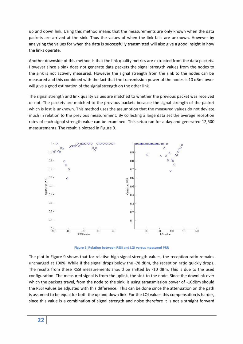
rates of each signal strength value can be examined. This setup ran for a day and generated 12,500
measurements. The result is plotted in Figure 9.
Figure 9: Relation between RSSI and LQI versus measured PRR
The plot in Figure 9 shows that for relative high signal strength values, the reception ratio remains
unchanged at 100%. While if the signal drops below the -78 dBm, the reception ratio quickly drops.
The results from these RSSI measurements should be shifted by -10 dBm. This is due to the used
configuration. The measured signal is from the uplink, the sink to the node, Since the downlink over
which the packets travel, from the node to the sink, is using atransmission power of -10dBm should
the RSSI values be adjusted with this difference. This can be done since the attenuation on the path
is assumed to be equal for both the up and down link. For the LQI values this compensation is harder,
since this value is a combination of signal strength and noise therefore it is not a straight forward
23
shift of the values. Therefore this measurement is insufficient to accurately measure the relationship
between the LQI and the packet reception ratio.
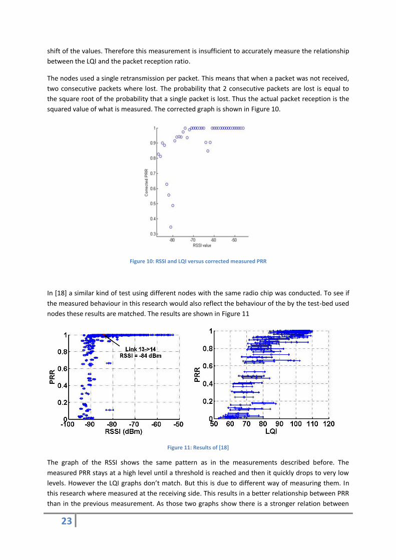
The nodes used a single retransmission per packet. This means that when a packet was not received,
two consecutive packets where lost. The probability that 2 consecutive packets are lost is equal to
the square root of the probability that a single packet is lost. Thus the actual packet reception is the
squared value of what is measured. The corrected graph is shown in Figure 10.
Figure 10: RSSI and LQI versus corrected measured PRR
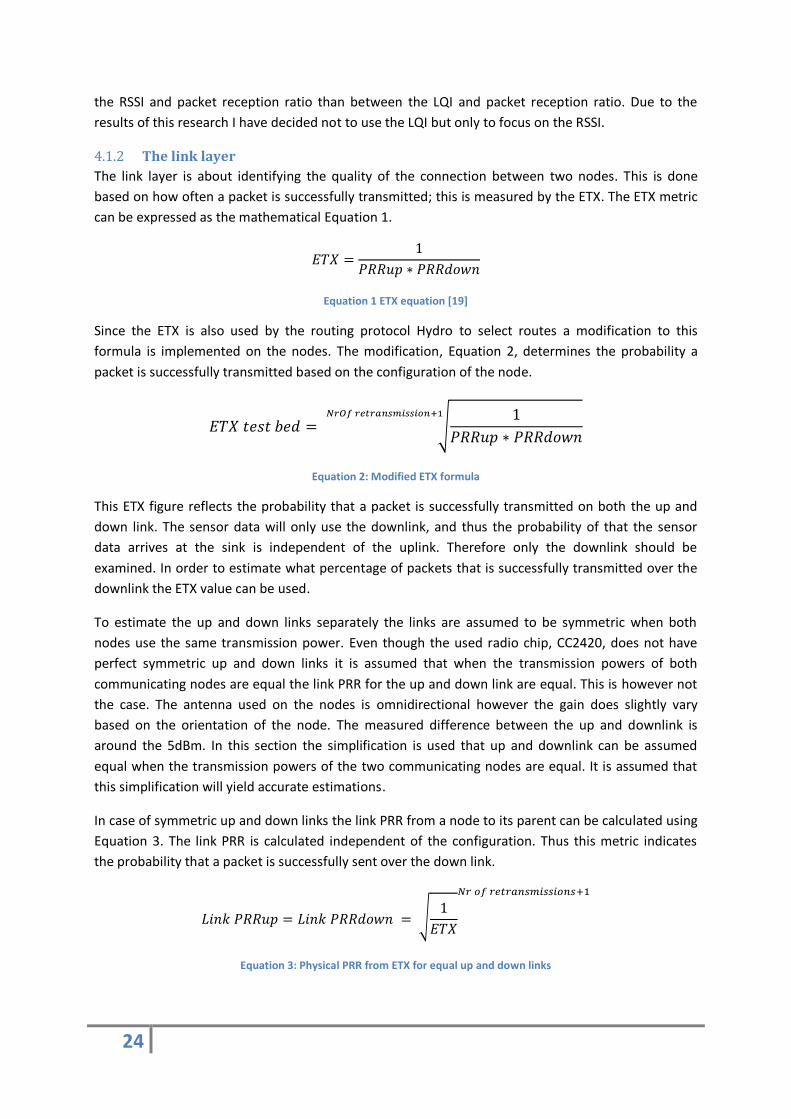
In [18] a similar kind of test using different nodes with the same radio chip was conducted. To see if
the measured behaviour in this research would also reflect the behaviour of the by the test-bed used
nodes these results are matched. The results are shown in Figure 11
Figure 11: Results of [18]
The graph of the RSSI shows the same pattern as in the measurements described before. The
measured PRR stays at a high level until a threshold is reached and then it quickly drops to very low
levels. However the LQI graphs don’t match. But this is due to different way of measuring them. In
this research where measured at the receiving side. This results in a better relationship between PRR
than in the previous measurement. As those two graphs show there is a stronger relation between
24
the RSSI and packet reception ratio than between the LQI and packet reception ratio. Due to the
results of this research I have decided not to use the LQI but only to focus on the RSSI.
The link layer 4.1.2
The link layer is about identifying the quality of the connection between two nodes. This is done
based on how often a packet is successfully transmitted; this is measured by the ETX. The ETX metric
can be expressed as the mathematical Equation 1.
Equation 1 ETX equation [19]
Since the ETX is also used by the routing protocol Hydro to select routes a modification to this
formula is implemented on the nodes. The modification, Equation 2, determines the probability a
packet is successfully transmitted based on the configuration of the node.
√
Equation 2: Modified ETX formula
This ETX figure reflects the probability that a packet is successfully transmitted on both the up and
down link. The sensor data will only use the downlink, and thus the probability of that the sensor
data arrives at the sink is independent of the uplink. Therefore only the downlink should be
examined. In order to estimate what percentage of packets that is successfully transmitted over the
downlink the ETX value can be used.
To estimate the up and down links separately the links are assumed to be symmetric when both
nodes use the same transmission power. Even though the used radio chip, CC2420, does not have
perfect symmetric up and down links it is assumed that when the transmission powers of both
communicating nodes are equal the link PRR for the up and down link are equal. This is however not
the case. The antenna used on the nodes is omnidirectional however the gain does slightly vary
based on the orientation of the node. The measured difference between the up and downlink is
around the 5dBm. In this section the simplification is used that up and downlink can be assumed
equal when the transmission powers of the two communicating nodes are equal. It is assumed that
this simplification will yield accurate estimations.
In case of symmetric up and down links the link PRR from a node to its parent can be calculated using
Equation 3. The link PRR is calculated independent of the configuration. Thus this metric indicates
the probability that a packet is successfully sent over the down link.
√
Equation 3: Physical PRR from ETX for equal up and down links

25
When the up and down links are not symmetric due to for example differences in transmission
power between the two communicating nodes this formula can be simplified to Equation 4
Equation 4: Physical PRR for unequal up and down links
Since one node is using more transmission power we assume that this link is of higher quality than
the other. When communication is still possible the higher quality link is assumed to result in a link
PRR of 100% and thus all the lost packets are assumed to be on the weak link. To verify the
relationship between the ETX and the PRR of the down link, the same type of measurement as with
the RSSI and LQI was used. This resulted in the following graph:
Figure 12: Relationship measured PRR versus the ETX
From this data, the estimated link PRR of the uplink can be determined. First the relation without
taking the number of retransmissions is examined. This is done to verify if the ETX metric accurately
estimates the probability that a packet is transmitted over the link.
Figure 13 Link PRR based on ETX values versus measured PRR

26
This graph, Figure 13, shows that the relationship between the estimated link quality and the actual
link quality. The graph shows that the ETX calculation on the nodes does take the number of
retransmissions into account when calculating the link quality. This is due to the linear relation
between the packet reception ratio and the ETX value while the nodes where using a single
retransmission. If the ETX calculation would not take the number of retransmissions into account this
graph would not have shown a linear relationship. A limitation of this metric is its precision. The
nodes report the ETX values with a precision of 0.1 Thus the first step from 1 to 1.1 reflects a change
in link quality of 9%. This is a big step when trying to estimate the quality of the link.
Another downside of this method is that it does not check the quality of the link from the node to its
parent, but looks at the link in both ways. When using the network to obtain sensing data the down
link is far more important, since on this link the data will travel from the nodes to the sink, than the
uplink. So it would be better when a method is used that only analyses the downlink instead of both
the up and downlink. When only the downlink is measured the assumption that the up and downlink
are equal is not needed to estimate the quality of the downlink which should lead to better
measurements of the downlink.
The transport layer 4.1.3
The transport layer is about the connectivity between a node and the sink independent of the node’s
location in the network and the configuration of the network. This connectivity is analysed based on
the number of received packets. The simplest method is to look at the average number of received
packets over a time span, but also more complex models exist. All those methods are coming from
the digital signal processing field. Each method results in a number between 0 and 100% quality
which should indicate the probability that a packet successfully travels through the network. This
metric is called the path quality. There is not much literature about path quality estimates. Therefor I
decided to use the link quality estimators to qualify the path quality.
In [2] different methods are introduced to estimate the link quality based on the actual received
packets. Some of these methods are mentioned here. Those methods work based on the information
whether a packet is received or dropped. Since the number of packets created by the nodes is
available the sink is able to determine this input and thus to use these models. To determine the
end-to-end PRR two different methods are presented. The first method is using the finite input
response filter (FIR) and the second method uses the infinite input response filter (IIR).
The finite input response filter is a filter type which uses a window. The most basic FIR filter is the
moving average filter (MAF). This filter uses a window of a certain length and returns the average
value over all inputs. The input in this situation is a Boolean value 1 if a packet was received and 0 if it
was not received. Calculating the average over multiple samples gives the most basic form of the
packet reception ratio; this method is also called the packet reception ratio. The formula to
determine the end-to-end PRR is given by Equation 5:
Equation 5: Packet reception ratio formula from [20]
27
In this equation the tau symbol indicates the round which is evaluated. The Link is a Boolean value
indicating whether the packet from that round is received or not, and the w is the size of the
window.
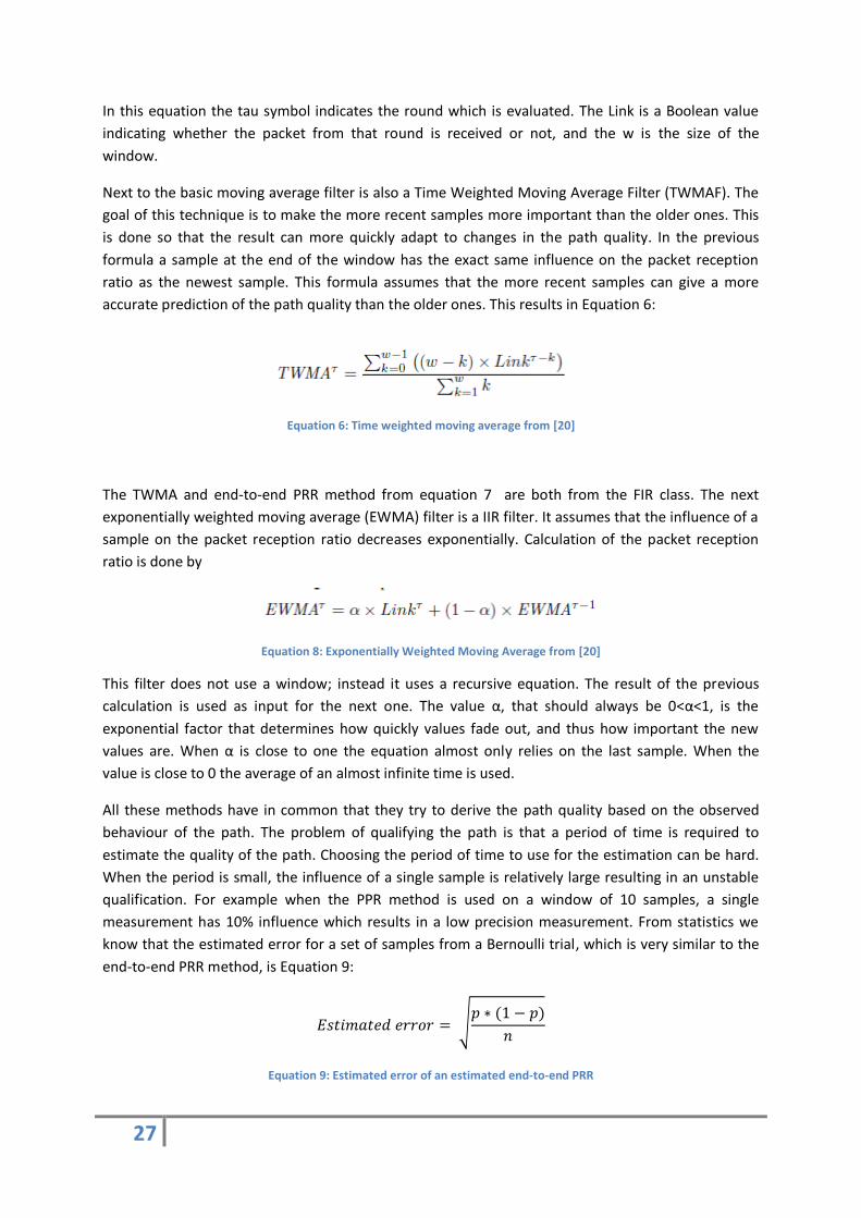
Next to the basic moving average filter is also a Time Weighted Moving Average Filter (TWMAF). The
goal of this technique is to make the more recent samples more important than the older ones. This
is done so that the result can more quickly adapt to changes in the path quality. In the previous
formula a sample at the end of the window has the exact same influence on the packet reception
ratio as the newest sample. This formula assumes that the more recent samples can give a more
accurate prediction of the path quality than the older ones. This results in Equation 6:
Equation 6: Time weighted moving average from [20]
The TWMA and end-to-end PRR method from equation 7 are both from the FIR class. The next
exponentially weighted moving average (EWMA) filter is a IIR filter. It assumes that the influence of a
sample on the packet reception ratio decreases exponentially. Calculation of the packet reception
ratio is done by
Equation 8: Exponentially Weighted Moving Average from [20]
This filter does not use a window; instead it uses a recursive equation. The result of the previous
calculation is used as input for the next one. The value α, that should always be 0<α<1, is the
exponential factor that determines how quickly values fade out, and thus how important the new
values are. When α is close to one the equation almost only relies on the last sample. When the
value is close to 0 the average of an almost infinite time is used.
All these methods have in common that they try to derive the path quality based on the observed
behaviour of the path. The problem of qualifying the path is that a period of time is required to
estimate the quality of the path. Choosing the period of time to use for the estimation can be hard.
When the period is small, the influence of a single sample is relatively large resulting in an unstable
qualification. For example when the PPR method is used on a window of 10 samples, a single
measurement has 10% influence which results in a low precision measurement. From statistics we
know that the estimated error for a set of samples from a Bernoulli trial, which is very similar to the
end-to-end PRR method, is Equation 9:
√
Equation 9: Estimated error of an estimated end-to-end PRR

28
For packet reception ratios this results in the following relation between packet reception ratios,
window sizes and estimated errors.
Equation 10: Relation between window size, packet reception ratio and estimated error
This graph shows that not only the smaller the window size the bigger the estimated error ratio but
also that the estimation shows a larger error rate when the path stability decreases. When for
example a window size of 100 is used and once per 5 minutes a sample is taken the oldest sample is
500 minutes or 8.3 hours old. Does an 8.3 hour old sample still contain valid information about the
current path’s state? So in general the smaller the window size the more accurate the information of
the samples but the more unstable the classification.
The goal of estimating the packet reception ratio is to be able to say something about the quality of
the path at the current time. To be able to see which methods and configurations have the best
reflection of what is going to happen in the future all methods are tested. The test consists of an
implementation of the method and a long run evaluation.
The evaluation is done by a deployed network where a node used 2 hops to connect the the sink.
Both hops contained a link that was of lower quality, on one node an average of 20% of the packets
was lost, the other one 5%. All the end-to-end PRR estimators from the node that relied on both of
these links are used for this analysis. The end-to-end PRR estimator is combined with the check
whether the next packet is successfully transported over the path. This check is related to the next
packet since the end-to-end PRR estimator is determined based on the previous values. In order to
make the analysis values independent of the estimator value is compared to whether the next packet
arrived. At the end the results are sorted in bins based on the path quality estimator. If the path
quality estimator is able to predict the future the average value of the check should match the
number of the estimator, or at least show a relation.
This dataset used for this evaluation is done with 13,921 samples. The node sent one sensor packet
every minute and a statistics packet every 5 minutes. The results are illustrated in Figure 14.

29
Figure 14 Relation between estimated path quality and actual path quality
This image illustrates that the large PRR methods did not give accurate estimations. This is probably
due to the time that measurements are related to the link quality. The PRR method with the window
of 20 samples does show a reasonable relation the link quality. For all three methods the ones that
are able to respond quickly performed better than the ones that try to be more accurate. Over all the
EWMA method with an exponential factor of 0.8 gave the best result. Just as with the path quality
prediction of the end-to-end PRR result, also for the TWPPR and EWMA the smaller window/smaller
coefficient implementations lead to better results.
Characteristics of a failing link 4.1.4
Next to analysing the characteristics of the parameters from the different communication layers to
the measured PRR, the characteristics of a link which is at the edge of its communication capabilities
is also considered. How does a link behave when it is close to losing connection and what quality
could the link still deliver in this situation?
As can be concluded from the physical layer analysis, the quality of the link can be well described by
the signal strength of the link. When this value comes close to the edge of it capabilities, in the test
bed -85 dBm, the quality of the link will quickly degrade. For the ETX such strong relations did not
appear. This however does not mean that those do not exist. The graphs plotted for analysis of the
ETX did not say anything about how often certain values occurred. Figure 15 shows a histogram of
the relationship between the link quality and how many measurements where received with its
corresponding value.

30
Figure 15: Histogram number of measurements and corresponding packet reception ratio
The histogram is constructed based on the communication of a single node transmitting its data back
to the sink with an RSSI value between -87dBm and -90dBm. The histogram shows on the x axis the
estimated PRR derived from the ETX value independent of its configuration. On the Y axis the
number of instances a value was measured is counted. What these graphs show is that when the
links are dropping packets, but there is still a working connection the majority of the time it is still
able to successfully transmit a packet. Over 60 % of the time the link is in a state in which it is able to
transmit over half of its packets. This shows that even when a link is of a bad quality it is still likely to
successful deliver packets with a probability over more than 50%. If the reception rate goes below
the 50% the link more likely to completely fail than to successfully deliver a low percentage of its
packets.
This information combined with the information that the link quality quickly drops when the RSSI
drops below -85dBm leads to a conclusion that if a link drops packets the packet loss is very likely to
be between 0% and 40%. Thus links that are the edge of its communication capabilities are still of a
good enough quality that the links can still successfully transmit data. Several experimental runs have
been conducted where nodes were pushed even further away from each other but a PRR of below
50% did not show up. Thus when the link quality is decreasing further total disconnection is more
likely to occur than extremely low link PRRs.
Configuring the network 4.2Once a WSN is physically deployed the configuration of the network is the next step. The possible
routes and their corresponding path qualities are highly determined by the physical deployment;
however the actual network quality relies on how the network utilises its resources.
Due to the properties of the radio communication the sensor network is most likely going to lose
packets. This should be acceptable and the network should compensate either in the application by
accepting the packet loss or in the network by increasing the reliability of the network. Therefore it is
important to consider will the application have its requirements for the WSN regarding the reliability
or the network and should the network use its resources to try to deliver the requirements.
Once a wireless network is deployed it is still highly configurable, properties like transmission power,
sensing frequency and retransmission rates are configurable post deployment. The goal of
configuring the WSN is to create a configuration that should meet the requirements. This is known as
quality of service support. To address this issue a Quality of Service (QoS) configuration framework is
proposed. This framework specifies different abstraction layers where the quality of the network is
measured and configured. For each layer, possible options are suggested to be able to change the
network’s configurations to the requirements of the application using it.
31
As the framework is targeted at the Nimbus WSN where nodes periodically send a sensing packet for
the application, no event-based configurations are taken into account. This framework could be
extended for event-based sensor networks but this is not addressed in this research.
The framework 4.2.1
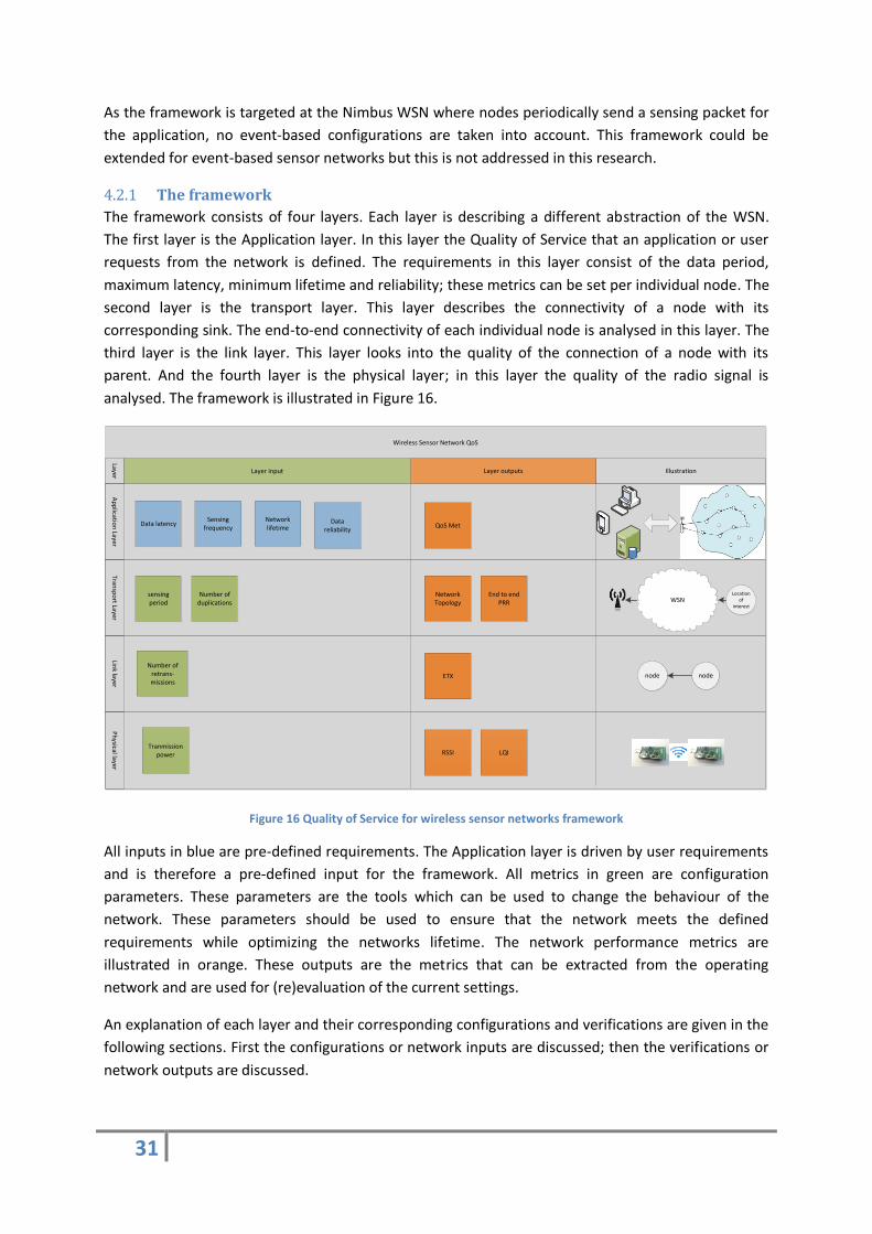
The framework consists of four layers. Each layer is describing a different abstraction of the WSN.
The first layer is the Application layer. In this layer the Quality of Service that an application or user
requests from the network is defined. The requirements in this layer consist of the data period,
maximum latency, minimum lifetime and reliability; these metrics can be set per individual node. The
second layer is the transport layer. This layer describes the connectivity of a node with its
corresponding sink. The end-to-end connectivity of each individual node is analysed in this layer. The
third layer is the link layer. This layer looks into the quality of the connection of a node with its
parent. And the fourth layer is the physical layer; in this layer the quality of the radio signal is
analysed. The framework is illustrated in Figure 16.
Wireless Sensor Network QoS
Ap
plicatio
n Layer
Transp
ort Layer
Link layer
Ph
ysical layer
Data latencySensing
frequency
sensing period
Network lifetime
RSSI LQI
Location of
interestWSN
nodenode
Layer input Layer outputs
QoS Met
Tranmission power
Network Topology
End to end PRR
ETX
Layer Illustration
Number of retrans-missions
Number of duplications
Data reliability
Figure 16 Quality of Service for wireless sensor networks framework
All inputs in blue are pre-defined requirements. The Application layer is driven by user requirements
and is therefore a pre-defined input for the framework. All metrics in green are configuration
parameters. These parameters are the tools which can be used to change the behaviour of the
network. These parameters should be used to ensure that the network meets the defined
requirements while optimizing the networks lifetime. The network performance metrics are
illustrated in orange. These outputs are the metrics that can be extracted from the operating
network and are used for (re)evaluation of the current settings.
An explanation of each layer and their corresponding configurations and verifications are given in the
following sections. First the configurations or network inputs are discussed; then the verifications or
network outputs are discussed.

32
The problem when configuring a network is how to respond to dynamic behaviours. Does the
network need to reconfigure as soon as a better configuration could be derived, or should this be
done periodically. The first option could lead to an unstable network which is reconfiguring
continuously, whereas the periodic reconfigurations could lead to unnecessary network failure, or a
waste of resources.
All sensor/network configurations are derived based on the application requirements. Thus the
required quality of the links depends on what the application requires form the network. When for
example the application does not need a high reliability then the loss of a packet in the network can
be tolerated, this in contradiction to the scenario where the application layer has a high reliability
requirement. In this section first the configuration options of each layer and their impacts on the
behaviour of the network are described. After this the method to suggest a new configuration is
introduced.
Application layer 4.2.2
In this research the type of sensing or actuation is not relevant since only the communication quality
of the network is considered. An application could define its requirements based on the following
parameters:
- Sensing period
- Reliability
- Network lifetime
The sensing period is the data dependency of the application; the reliability regards the
communication quality of the network whereas the network lifetime is a resource restriction. The
reliability and the network lifetime restrict each other which could cause the network to be un-
configurable. When there is no configuration that matches all the requirements the deployment
should be re-evaluated. The framework that has been developed will only take the reliability into
account, and is thus not restricted by lifetime constraints. Next to that it does not take throughput
into account. The used communication channel has a throughput of 250 kbps while a packet is more
or less 120 bytes long. Per second more than 2000 packets could be transmitted. The used network
for buildings has typical sensing periods in the seconds or minutes. The throughput is in this case thus
of not critical. Latency is not taken into account in this framework because of the incapability of the
network to measure it. However when the framework would be extended further research should
include the throughput, lifetime, and latency.
4.2.2.1 Sensing period
The sensing period specifies the amount of time between two consecutive readings from a location
of interest. This can differ for each sensor, or each type of sensor depending on the application.
4.2.2.2 Reliability
Due to the lousy properties of the radio channel an absolute certainty that packets arrive can never
be given. Therefore the application should specify a minimum reliability. This reliability is the
percentage of readings that are successfully delivered to the application.
4.2.2.3 Network lifetime
The lifetime of the network defines the maintenance work required to keep the application running.
For many applications a minimum operation time should be guaranteed. The deployment should be

33
aware of this minimum time, and try to adapt its configuration to meet the requirement. The lifetime
of a node is strongly related to the activity of the radio chip. By lowering the transmission power
and/or decreasing the load on the radio chip the lifetime of the node can be extended. The lifetime
of the network has multiple definitions, but all of them have in common that nodes should live as
long as possible.
4.2.2.4 Verification of the reliability
To measure the reliability of a sensor a moving average filter is used. At the end of every period a
check is done whether the sensor data from that period is received or not. This method checks
whether within the period one or multiple sensor readings are received does not matter, since
according to the specification at least one reading per period is required. The moving average filter
will determine after each period the reliability of the link at that moment of time.
The outcome heavily relies on the size of the window. A large window will have a high accuracy, but
will also allow longer bursts of packet loss. For example a reliability of 95% and a window size of 100
can accept at most 5 consecutive missed packets and has an precision of 1%. A more accurate
estimation is not possible using a windows size of a 100 samples. When a window size of 1000 is used
the maximum consecutive missed packets is 50 and will have a precision of 0.1%.
The size of the window will have to be set according to the application’s requirement to be sure that
the required accuracy can be reached and that the maximum number of possible consecutive missed
packets does not exceed the specification. Multiple windows can be created per node, for example
when different sensors need different windows.
The transport layer 4.2.3
Once the application requirements are set the transport layer should ensure that despite the
characteristics of the WSN the application gets the service required. To do so the operation metrics
from the network are used as inputs and configuration settings are used to try to let the network
deliver the required quality.
In the framework, the assumption is made that the links can be modelled as a Bernoulli trial using the
PRR of the links. In order to use a Bernoulli trial it should be possible to model the loss of data a
probability p and the events of data loss should be unrelated to each other. This probability is
assumed to be equal to the link PRR. This method has also been used to simulate link losses for WSN
by other researchers [21]. All formulas used in this section come from the Bernoulli theory and
mathematical rewrite rules.
The option on this layer to change the behaviour of the network is to configure the number of
duplicated packets transmitted per period. When the reliability requirement is not met, the amount
of lost packets in the network is too high. This can be compensated by injecting multiplications of
packets.
4.2.3.1 The number of duplications
The application requires periodic updates from a sensor. The minimum update frequency is defined
by the application. Only a case where no packets are lost in the network will the requirement be met
with 100% reliability. In all other cases a chance of not meeting the requirements is present. The
probability that a packet is not delivered to the sink is defined by Equation 11. This equation assumes
that a sensor reading is transmitted using a single packet, thus not fragmented which is the case in

34
the test bed. Based on this assumption the probability that a packet is delivered successfully is equal
to the probability that a sensor reading is delivered successfully.
Equation 11 Percentage of Application data interval deadlines met
To ensure the application requirement is met, it might be necessary to send more than one packet
per period. The probability that the requirement is met could be calculated based on the probability
that a packet gets lost which equals 1 minus the packet reception ratio to the power of the number
of packets sent per interval. The end-to-end PRR options introduced in 4.1.3 can be used in this
formula for the end-to-end PRR. This number is defined by the network; the number of duplications
is the configuration parameter in this formula. Changing the number of duplications can be used to
meet the reliability requirement
Since the PRR is a metric that can be derived from the active deployment and the minimum reliability
is specified by the application only the number of duplications can be configured to meet the
requirement. Rewriting Equation 11 gives the following result for setting the sensing interval time.
⌈
⌉
Equation 12 Minimal sensing interval length
The following chart shows the impact of the packet reception and the minimum reliability influence
on the sensing interval period.
Figure 17 Relationship between end-to-end PRR and minimum reliability
This graph shows on the x axis the packet reception ratio of the link from a node to the sink; this is
the metric that will be determined by the network. The y axis shows the required number of
retransmissions to meet the application requirement, configuration parameter of the network. The
four different lines in this graph relate to four different application requirements. So for example the

35
network has an end to end packet reception ratio of 0.8 and the application requires 98% hit ratio.
Then the required number of duplications equals:
⌈
⌉
So with these settings the number of injected packets of the node should be three times higher than
the required minimum number in order to meet the requirements of the application.
To define this value, the relation between the load on the nodes and the reliability needs to be taken
into account. The closer the hit ratio comes to 100%, the higher the load on the nodes which results
in a lower lifetime. So a trade-off between lifetime of the network and quality of the network should
be made.
Next to the minimum number of duplications there are also a maximum number of duplications. The
nodes are all limited to the amount of energy they are allowed to use due to the lifetime
requirement. To exactly determine the maximum number of retransmissions is challenging. To do so
the relationship between a nodes lifetime and sensing period and number of duplications should be
determined. A node uses more power when transmitting more packets, but the lifetime does not
only depend on the number of packets sent. Therefore, a model is required to come up with a good
maximum sensing frequency. This is research where other people within Nimbus are working on and
therefore I did not go any deeper into this subject than only stating that the sensing period and
number of duplications will be bounded on both sides. This research focuses on the restrictions on
one side. Since the lifetime of the network is not included into this version of the framework it is only
stated that the number should be kept at a minimum and in a later version restrictions could be
made on this number.
The link layer 4.2.4
The link layer defines the quality for the communications for a node to its parent. The quality of the
link is defined by its packet reception ratio. The packet reception ratio depends on the quality of the
physical link and the number of retransmissions for a packet whereas the delay depends on the duty
cycle time. The quality of the physical link will define the probability that a single packet is
transmitted successfully and the combination between the probability that a packet is transmitted
successfully and the number of retransmissions will define the link PRR. The end-to-end PRR of an
end to end link can be determined by the product of the packet reception ratios of all the individual
links on the path from a node to the sink, see Equation 13. When improving the packet reception
ratio of a link all nodes that use that link will benefit from this improvement.
∏
Equation 13 End to end packet reception ratio
To improve the quality of a link the same principle is used as for the transport layer. To improve the
link quality multiple instances of the packet will be transmitted in order to create a stronger link. On
the link layer the packets will not simply be duplicated but rather a retransmission of the same
packet, and is only transmitted when an acknowledgement is not received.

36
When a node sends a packet to its parent it expects that the parent will send back an
acknowledgement after it successfully received the packet. If a node does not receive the
acknowledgement after a pre-set period of time it retransmits that packet. The maximum number of
retransmissions is bounded in order not to overflow the nodes memory, to maintain lifetime and not
to block the communication channel an infinite amount of time for transmitting an unsuccessful
packet.
This bounded number of retransmissions is what should be configured at this layer. When increasing
the number of retransmissions the link quality will increase and lowering it enables the node to live
longer. Therefore, the minimum required number of retransmissions should be found that would still
maintain an acceptable level of link quality.
The formula for the link quality is almost the same as for the end-to-end packet reception ratio.
However the packet reception ratio of a single link is derived from the ETX value. In section 4.1.2 the
relation between the ETX value and the link reception ratio is discussed. This described method is
used to obtain the link packet reception ratio. Therefore the formula becomes
Equation 14: Link quality
The impact of the number of retransmissions on the link PRR is illustrated in Figure 18.
Figure 18: Relation between the number of retransmissions and the link packet reception ratio
This figure shows that the higher the number of retransmissions is the lower the physical PRR needs
to be to maintain a good link PRR.
As is stated in section 4.1.4, a link will barely ever drop below a packet reception ratio of 0.6.
Therefore a threshold for the maximum recoverable Physical PRR can be set at 0.6. So recovering
from physical PRRs of under 0.6 is unnecessary; those links will be qualified as unstable. Those links
qualities should be avoided and when they occur a redeployment should be considered. Since a
retransmission rate of 3 with a physical PRR of 0.6 will give a link PRR of 0.97 there is no need to use
higher retransmission rates than 3.

37
If a retransmission rate of 3 is used and a transmitter is using its maximal power and the link is still
not meeting its requirements the link will be qualified as unstable and could cause the node and all
nodes it relays the data for to miss their application requirements.
The physical layer 4.2.5
The configuration option for the physical layer consists of the adaptation of changing the
transmission power. Since the majority of a nodes energy is consumed by receiving and transmitting
data, reducing the transmission power shall have great influence on the lifetime of a node. Table 1
shows the relation between the configured transmission power and the current drawn by the
transmitter.
Transmission power in dBm Current drawn
0 17.4
-1 16.5
-3 15.2
-5 13.9
-7 12.5
-10 11.2
-15 9.9
-25 8.5 Table 1: Transmission power versus current drawn [22]
As was concluded in section 4.1.1 it is important to maintain signal strength at the receiving node of
more than -85 dBm in order to maintain a good link quality. This should thus be guaranteed when
lowering the transmission power of a node, or else the communication link between the two nodes
shall suffer from the reconfiguration.
Since all nodes measure the RSSI values of all links and report those back to the sink, these values are
known for evaluation of the links. When evaluating the transmission power of a node all incoming
and outgoing links should be taken into account. Only when the signals on all links are high enough to
lower the transmission power should it be lowered. And the other way around is the same, when
there is one link whose received power is too low the transmission power of the node should be
increased. By doing this for all nodes the transmission powers of all nodes can be determined, and
the lifetime of some of the nodes can be increased without the loss of quality for the network.
Determining the required configuration 4.3The relationship between the possible configurations and the effect on the behaviour of the network
is known a model to determine the configuration of the network is the next step. The configuration
of the network will be done in two independent stages. One stage determines the transmission
power of all the nodes, the physical layer configuration, and the other stage determines the number
of retransmissions and packet duplications, the link layer and the transport layer configurations.
The physical layer configuration 4.3.1
The configuration of the physical layer takes as input the RSSI values of all links. It is known from the
analysis of the physical layer that as long as the received RSSI is higher than -85 dBm the quality of

38
the link will remain the same. This is important due to this property the configuration of the physical
layer and the link and transport layer can be done independently of each other. The goal of the
configuration will be to use a minimum transmission power and maintaining the RSSI values of all
links above the -85 dBm.
For setting the transmission power a limited number of possible transmission powers are used. The
possible settings are:
- 0 dBm
- -7 dBm
- -15 dBm
To determine a node’s transmission power configuration the following three checks are used:
These checks involve all incoming and outgoing links on a node. Since a node requests an
acknowledgment after sending a packet is important that the link quality for as well the uplink as the
downlink are of a good quality.
All three checks will return a Boolean value on whether the value formula was true of false. The first
check that returns true determines the configuration for that node. Thus when all links will remain
higher than -85 dBm after subtracting 15 from the current signal, -15 dBm will be used as
transmission power. When none of the three checks return true the link will be configured with the
maximum transmission power but the link is likely to have a weak link. When this occurs it is up to
the routing protocol to decide whether there are other links which can be used that might have a
better quality.
The link layer and transport layer configuration 4.3.2
The number of retransmissions, link layer, on a link and duplications of a packet, transport layer, will
be configured together since both configurations are strongly related. The goal of configuring the link
and transport layer is to ensure the reliability of the nodes. The reliability was defined as the
probability that per sensing period one packet of a node is received by the sink.
Both the duplications and retransmissions will impact the reliability of the nodes. Next to that they
will also impact the load on the network and thus its lifetime. Therefore, it is important that a
minimum number of retransmissions and duplications are used while maintaining the required
reliability of the nodes.
The relationship between configuration options and the reliability was already given in section 4.2.4
for the link layer and section 4.2.3 for the transport layer. The relation between the load on the
network and the two configuration options is given by Equation 15 for the duplications and Equation
16 for the retransmissions.
∑
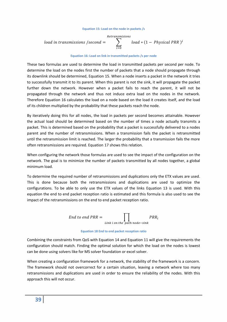
39
Equation 15: Load on the node in packets /s
∑
Equation 16: Load on link in transmitted packets /s per node
These two formulas are used to determine the load in transmitted packets per second per node. To
determine the load on the nodes first the number of packets that a node should propagate through
its downlink should be determined, Equation 15. When a node inserts a packet in the network it tries
to successfully transmit it to its parent. When this parent is not the sink, it will propagate the packet
further down the network. However when a packet fails to reach the parent, it will not be
propagated through the network and thus not induce extra load on the nodes in the network.
Therefore Equation 16 calculates the load on a node based on the load it creates itself, and the load
of its children multiplied by the probability that these packets reach the node.
By iteratively doing this for all nodes, the load in packets per second becomes attainable. However
the actual load should be determined based on the number of times a node actually transmits a
packet. This is determined based on the probability that a packet is successfully delivered to a nodes
parent and the number of retransmissions. When a transmission fails the packet is retransmitted
until the retransmission limit is reached. The larger the probability that a transmission fails the more
often retransmissions are required. Equation 17 shows this relation.
When configuring the network those formulas are used to see the impact of the configuration on the
network. The goal is to minimize the number of packets transmitted by all nodes together, a global
minimum load.
To determine the required number of retransmissions and duplications only the ETX values are used.
This is done because both the retransmissions and duplications are used to optimize the
configurations. To be able to only use the ETX values of the links Equation 13 is used. With this
equation the end to end packet reception ratio is estimated and this formula is also used to see the
impact of the retransmissions on the end to end packet reception ratio.
∏
Equation 18 End to end packet reception ratio
Combining the constraints from QoS with Equation 14 and Equation 11 will give the requirements the
configuration should match. Finding the optimal solution for which the load on the nodes is lowest
can be done using solvers like for MS solver foundation or excel solver.
When creating a configuration framework for a network, the stability of the framework is a concern.
The framework should not overcorrect for a certain situation, leaving a network where too many
retransmissions and duplications are used in order to ensure the reliability of the nodes. With this
approach this will not occur.
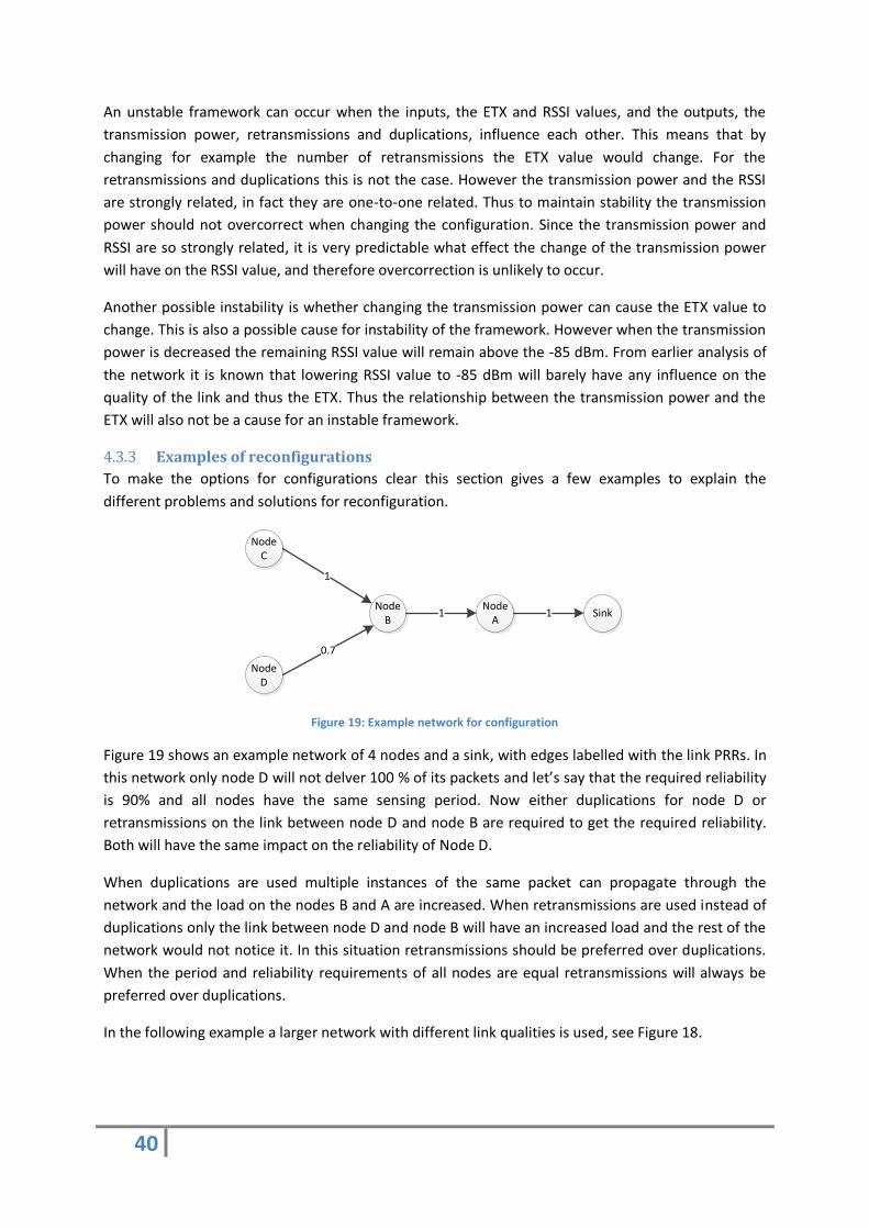
40
An unstable framework can occur when the inputs, the ETX and RSSI values, and the outputs, the
transmission power, retransmissions and duplications, influence each other. This means that by
changing for example the number of retransmissions the ETX value would change. For the
retransmissions and duplications this is not the case. However the transmission power and the RSSI
are strongly related, in fact they are one-to-one related. Thus to maintain stability the transmission
power should not overcorrect when changing the configuration. Since the transmission power and
RSSI are so strongly related, it is very predictable what effect the change of the transmission power
will have on the RSSI value, and therefore overcorrection is unlikely to occur.
Another possible instability is whether changing the transmission power can cause the ETX value to
change. This is also a possible cause for instability of the framework. However when the transmission
power is decreased the remaining RSSI value will remain above the -85 dBm. From earlier analysis of
the network it is known that lowering RSSI value to -85 dBm will barely have any influence on the
quality of the link and thus the ETX. Thus the relationship between the transmission power and the
ETX will also not be a cause for an instable framework.
Examples of reconfigurations 4.3.3
To make the options for configurations clear this section gives a few examples to explain the
different problems and solutions for reconfiguration.
Node A
Node B
Node C
Node D
Sink
1
0.7
1 1
Figure 19: Example network for configuration
Figure 19 shows an example network of 4 nodes and a sink, with edges labelled with the link PRRs. In
this network only node D will not delver 100 % of its packets and let’s say that the required reliability
is 90% and all nodes have the same sensing period. Now either duplications for node D or
retransmissions on the link between node D and node B are required to get the required reliability.
Both will have the same impact on the reliability of Node D.
When duplications are used multiple instances of the same packet can propagate through the
network and the load on the nodes B and A are increased. When retransmissions are used instead of
duplications only the link between node D and node B will have an increased load and the rest of the
network would not notice it. In this situation retransmissions should be preferred over duplications.
When the period and reliability requirements of all nodes are equal retransmissions will always be
preferred over duplications.
In the following example a larger network with different link qualities is used, see Figure 18.

41
Node C
Node B
Node D
SinkNode
A
1
1
0.7 1
Node E
Node F
1
1
Figure 20: Example network 2 for configuration
In this example the sensing periods of all nodes except node D are 1 packet per second and the
reliability requirement is 85%. For node D the requirement is to deliver once per 8 seconds a packet
with 95% reliability.
The load on the nodes is now without duplications and retransmissions
When optimizing this network for the minimum total load of the network node B should be
configured using 1 retransmissions and node D with one duplication. This will result in Table 2
showing the load on the network, and the corresponding reliabilities.
Table 2: Network load en reliability after reconfiguration
The complete load of the network becomes 15.6 transmitted packets per second and all reliabilities
are matching the requirements. This example shows the use of duplications and retransmissions
related to the QoS requirements of the nodes, and that the optimum can be found combining both.
Duplications will be used when the node that has a weak downlink or one of its children has a higher
reliability constraint that the other. By increasing the number duplications on that node could
prevent unnecessary high retransmissions, and could lead to a lower load on the network.
Node Load in packets
Node E 1/1 + Load children * link PRR = 1
Node F 1/1 + Load children * link PRR = 1
Node C 1/1 + Load children * link PRR = 1 +1 +1 = 3
Node D 1/8 + Load children * link PRR = 0.16
Node B 1/1 + Load children * link PRR = 1 + 3*1 + 0.125 *1 = 4.16
Node A 1/1 + Load children * link PRR = 1 + 4.125*0.7 = 3.89
Node Load in transmissions per second over link Reliability
Node A 4.8 1
Node B 5.2 0.91
Node C 3 0.91
Node D 0.25 0.99
Node E 1 0.91
Node F 1 0.91

42
Verification of the analysis and configurations on real deployment’s 4.4To see how the theory described previously in this document on analysis and configuration of
wireless networks data from a number of deployments were taken into account. The deployments
were carried out in two locations over a period of multiple days to see how they behave and whether
this matches the previously described expectations. The analysis of the deployments is made in this
section.
The first location contains a deployment where 8 nodes are used to create a communication network
over multiple floors of an office building in Grenoble. In the second deployment 10 nodes are used to
create a sensing network in the Nimbus building in Cork.
Both deployments contain a small number of nodes but this is also due to the small size of the
buildings. The use of more nodes would have led to a denser deployment where the routing protocol
is able to find high quality routes and the network is likely not to drop packets Therefore relatively
small sized deployments where chosen.
The Grenoble deployment 4.4.1
In Grenoble multiple test deployments were executed as part of the EU FP7 SCUBA project . And the
data of this deployment has been made available for analysis. A number of configurations were
deployed in the same building over 2 floors using 8 nodes and a gateway. All deployments were
carried out in the same building across two floors. To demonstrate the analysis capabilities of the
proposed framework, this section will present the evaluation of two configurations in terms of the
quality of the deployment.
4.4.1.1 Deployment 1
The map of the first deployment is illustrated in Figure 21.
Figure 21 Map of deployment 1 in Grenoble

43
The deployment covers two floors of the building. The nodes x0b44 and x0b45 connect the different
floors. Thus the connections between those two nodes and the connection of x0b44 to the gateway
are crucial for all the nodes on the first floor, since all packets from the first floor will be sent over
these links. The standard configuration used to deploy networks is to transmit at full power and to
use at most 2 retransmissions per packet. This is a pessimistic approach but it is good to use it as a
starting point. When there are links of a lower quality the network is still likely to be able to transmit
its data over this link.
A first look at the average end-to-end PRR and ETX values of the links as described in 4.1.2 and 4.1.3
is presented in Figure 22. This is for all nodes over the complete deployment period and shows that
node 0b45 lost 4% of its packets, and the other nodes on the first floor 0b47, 0b48 and 0ab46 lost
almost half of their packets. From this, it is likely that a fraction of the data is lost on the link between
0b45 and 0b44, but that the link between 0b47 and 0b45 is of a worse quality.
Figure 22 Packet reception ratios of deployment 1 in Grenoble
The ETX numbers are matching that analysis. The more packets were lost on the links the higher the
ETX values are. The last step of the analysis is to match it with the RSSI values. From section 4.1.2 we
know that it is possible to derive the packet reception ratio from the ETX values.
√
√
√
√
9

44
Doing this shows us that the actual measured packet reception ratio on the link 0b45-0b44 is a match
with the actual packet reception ratio. However the other link 0b47-0b45 the calculated packet
reception ratio does not match the nodes packet reception ratio. The estimated packet reception
ratio of the node 0b47 is 0.77 and the packet reception ratio of the node equals 0.57.
∏
There is a good explanation for the difference in those two numbers. When measuring the link ETX
the sink is dependent on the arrival of the packets from the node. When over a longer period no
packets arrive a new ETX value is unknown while the link is of a lower quality. When using the
average over the entire period and only values of lower quality are missing, the result will become
too optimistic. It is therefore recommended that when using the metrics from the network, a small
period of time should be evaluated to reduce this impact.
Next to the packet reception ratio and link ETX values the RSSI is a good link quality indicator. The
average RSSI value of the link between 0b45 to 0b44 is -83 dBm. This should be sufficient to maintain
a good quality link. But when looking at the plot of the RSSI value over time, Figure 23, it becomes
clear that during the day the signal strength is lower than during the night times. The same pattern is
expected for the link 0b47 to 0b45, but when a link that is at -90 dBm degrades further the
connection is lost and no new readings are obtained by the sink. It can be concluded that the
behaviour of the network is flexible since the values of the RSSI can vary by 5 to 10 dBm. Thus, when
using the configuration framework, the re-evaluation of the configuration should be a continuous
process. A single configuration for a deployment will not be sufficient, as the dynamics of the
network to high.
Figure 23: RSSI plot of deployment 1 in Grenoble
4.4.1.2 Deployment 2
For the second configuration the node which was located close to the base station was moved to the
first floor in order to create a more robust connectivity in that area, which should improve the
delivery of packets to the sink. The second deployment is illustrated in Figure 24.

45
Figure 24 Map of deployment 2
The most used links of the deployment, the node packet reception ratio sand RSSI values are
illustrated in Figure 25.
Figure 25: Deployment 2 RSSI and end-to-end PRR
A remarkable thing from this redeployment is that the node 0b44 is now loosing 30% of its packets
whereas in the first deployment the exact same location of the node was used and during that time
period no data was lost. All other nodes that rely on this node to forward their data show the same
losses, it is very likely that these losses are caused by the inability of node 0b44 to reach the sink. The
RSSI value of 0b44 is -79 dBm and does not indicate the possibility of a bad link. Normally links with
this value would be able to operate at a high quality.
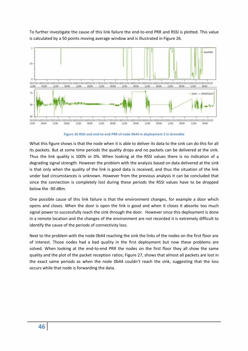
46
To further investigate the cause of this link failure the end-to-end PRR and RSSI is plotted. This value
is calculated by a 50 points moving average window and is illustrated in Figure 26.
Figure 26 RSSI and end-to-end PRR of node 0b44 in deployment 2 in Grenoble
What this figure shows is that the node when it is able to deliver its data to the sink can do this for all
its packets. But at some time periods the quality drops and no packets can be delivered at the sink.
Thus the link quality is 100% or 0%. When looking at the RSSI values there is no indication of a
degrading signal strength. However the problem with the analysis based on data delivered at the sink
is that only when the quality of the link is good data is received, and thus the situation of the link
under bad circumstances is unknown. However from the previous analysis it can be concluded that
since the connection is completely lost during these periods the RSSI values have to be dropped
below the -90 dBm.
One possible cause of this link failure is that the environment changes, for example a door which
opens and closes. When the door is open the link is good and when it closes it absorbs too much
signal power to successfully reach the sink through the door. However since this deployment is done
in a remote location and the changes of the environment are not recorded it is extremely difficult to
identify the cause of the periods of connectivity loss.
Next to the problem with the node 0b44 reaching the sink the links of the nodes on the first floor are
of interest. Those nodes had a bad quality in the first deployment but now these problems are
solved. When looking at the end-to-end PRR the nodes on the first floor they all show the same
quality and the plot of the packet reception ratios; Figure 27, shows that almost all packets are lost in
the exact same periods as when the node 0b44 couldn’t reach the sink, suggesting that the loss
occurs while that node is forwarding the data.

47
Figure 27: Packet reception ratios of all nodes on the first floor deployment 2 Grenoble
What can be concluded from this deployment analysis is that analysing the network is not straight
forward. Using the analysis tool a summary of the performance is given, however due to the
dynamics of the network this summary will not perfectly reflect how the network is behaving.
However, the in section 4.1 described metrics to analyse the network do reflect the network qualities
at specific moments in time. Thus analysing the network can be done using these metrics only the
dynamic aspects of the network should be taken into account.
The Nimbus deployment 4.4.2
For the Nimbus deployment, 10 nodes were used and dispersed across a single floor. To see if those
nodes could create a fully connected network the deployment tool was used. After deployment the
analysis was made and reconfiguration of the nodes was suggested and implemented. All steps are
discussed in this section.
4.4.2.1 The initial deployment:
As a starting point 10 nodes and a single sink were spread over the first floor of the Nimbus building.
To ensure connectivity, the deployment tool was used. The output of the deployment tool is
illustrated in Figure 28.
Figure 28: Topology and link quality estimation of deployment tool
According to the tool all nodes will be connected to the sink. Therefore, this will be the physical
deployment which is used for the tests. As a starting point, all nodes are configured at maximum
transmission power and two retransmissions.

48
4.4.2.2 Analysing the deployment
The deployment ran for one day. This should be enough to get a first impression of what the link
qualities are and to see what new configuration can be derived from the deployment information.
The packet reception ratios and RSSI values are illustrated in Figure 29.
Figure 29: Packet reception ratio s and RSSI values of deployment 1 in Nimbus
As this figure shows, all nodes managed to deliver 100% of their packets, and no links had signal
strengths lower than -85 dBm. Based on this initial deployment a reconfiguration is determined
which will optimize the lifetime of the network without compromising its quality.
4.4.2.3 The reconfiguration
As described in subsection 4.3 is reconfiguration done in two parts. The first part is to determine the
transmission power settings of the nodes and after that the number of duplications and
retransmissions are determined.
To determine the transmission power of the nodes the current signal strength values are important.
When lowering the transmission power the remaining signal should remain more than -85 dBm. Thus
the following table shows for each link the RSSI values of the worst connection. The worst
connections of each node is enough for the analysis since as shown in the section 4.3.1 all incoming
and outgoing links from a node should remain higher than -85 dBm when lowering the transmission
power. Thus only looking at the worst link is enough.
Node Worst RSSI value Check -15 dBm Value -15>-85
Check -7 dBm Check 0 dBm
A01 -81 False False true
A02 -76 False False true
A03 -61 True True true
A04 -81.2 False False true
A05 -82 False False true
A0A -73 False True true
A0B -68 True True true
A0C -81.2 False False true
A0D -80 False False true
A0E -55 True True True Table 3: Transmission power checks
Based on Table 3 the conclusion can be made that the transmission powers of nodes A01, A02, A04,
A05 A0C and A0D should remain unchanged. The transmission powers of then nodes A03 can be
lowered with 7 dBm and A03, A0C and A0E with -15 dBm without compromising on the link qualities.

49
Determining the number of retransmissions and duplications is easy in this situation. Since all nodes
delivered 100% of their packets, no duplications and retransmissions need to be used.
4.4.2.4 Deploying the reconfigured deployment
After all nodes were reprogrammed and put pack on their positions the network should start
rebuilding the network. However the test bed is only tested on a single configuration this
configuration is that all nodes use the same transmission power and 2 retransmissions. For other
configuration no extensive testing and debugging was done yet. Now that different transmission
powers are used in the same network, building the routing tables does not work properly.
All nodes which can reach the sink in a single hop where successfully connected to the sink. But for
example node A0C which used node A04 to forward its packets does not connect anymore while
those nodes are still using full transmission power. Since the transmission power has not changed
those nodes should still be able to connect to each other and form a network. The reason why this
isn’t happening is not clear.
Due to the issues regarding rebuilding of the network no data could be retrieved to verify the quality
of the network after reconfiguring the nodes. Since part of the assignment was to use the test bed as
is, verification of the framework is challenging.
Problems with the wireless sensor network test bed 4.4.3
As the previous section already stated challenges regarding the use of test bed in different
configurations raised. During the tests I have performed, three types of unexpected behaviour where
found. These types regard the use of the network with nodes using different transmission power
setting, node that use no retransmissions and links that come close to a connectivity loss. All three
are described here.
4.4.3.1 Multiple transmission powers in a single network
The issue with multiple transmission powers in a single network concerns the creation of routes in
the network. This issue can be explained using two nodes and a sink of which one node is using a
lower transmission power, node A. The other node, node B, and the sink will use the same higher
transmission power and are both able to transmit packets to the node with the lower transmission
power. However Node A due to its lowered transmission power is unable to transmit data to the
sink. This situation is illustrated in Figure 30.
Node A
Node B
Sink
Figure 30: 3 nodes connectivity problem
Node A would preferably connect to the sink instead of connecting through node B. However, this
connection is not possible since node A is using a lower transmission power and it therefore unable
to reach the sink. But what I think that will happen is that node A receives messages of the sink and
that it thus assumes that the sink is within range of node A. This causes node A to try to send its
packets directly to the sink whereas it due to its lower transmission power is unable to reach it. This

50
leaves node A unconnected while it could connect to the network using node B. I ran into this
multiple transmission power problem multiple times and in different configurations and locations
and the same pattern was seen over and over again. My conclusion form this was that this test bed
only supports a single transmission power level for each node.
4.4.3.2 No retransmissions
The problem when no retransmissions are used is that the network does not measure its ETX
according to its definition. No matter what the quality of the link is the ETX value will always remain 1
while it should indicate the quality of the link. To illustrate this I placed a node at a location where
during the night the link was of a good quality and during the day packets where lost on the link. This
node is directly connected to the sink thus only one link is involved in the communication. Both the
packet reception ratio and the ETX value are plotted in Figure 31.
Figure 32: Packet reception ratio and ETX of a weak link with 0 retransmissions
As this graph shows, the end-to-end PRR drops to about 30% while the ETX remains 1. Since the ETX
is related to the link quality it should show the same pattern as the end-to-end PRR. Using the ETX
value to qualify the link quality becomes more challenging when this value cannot be used when a no
retransmissions are used the link.
Next to analysis of the links, also the network itself will suffer from this. The routes in the network
are determined based on the ETX values. When those values will not reflect the actual link qualities
the network is unable to determine which routes lead to a strong topology and it will always select
the shortest route independent of the quality of the links.
My hypothesis is caused by the fact that the ETX values are measured depending on the configured
number of retransmissions on the nodes. Thus the ETX reflects the probability that a packet is
successfully transmitted of the link in the current configuration. Thus the higher the number
configured retransmissions the lower the ETX value will be. This suggests that the ETX value is also
determined based on how often and how many retransmissions are used to send a packet over the
link, but when a node is configured not to use retransmissions it will never use one and thus no
increase in ETX will be measured since each packet will only be transmitted once.

51
4.4.3.3 Low quality links with retransmissions
The last problem that I have encountered occurred in the situation when a node connects to for
example the sink and there are no other nodes to use to forward the node’s data. The used location
of the node is the same as in the previous problem description only now 2 retransmissions are used.
Since the number of transmissions per packet is increased I would expect that the node is able to
successfully deliver more of its packets and to see variation in the ETX values. However the node
disconnects itself after a couple of minutes and does not reconnect to the sink. When moving the
node closer to sink, and the link quality increases it can reconnect. When moving the node back to its
old position results again in an active link for a couple of minutes after which it disconnects again.
What I think causes this is that a node uses a threshold value after which it assumes that the link is of
a too bad quality to use and disconnects from the link. When there are no other links to connect to
the node remains unconnected to the network. The link quality is measured in ETX and I think that a
threshold is set on the ETX value. This idea is strengthened by the fact that when placing a node at
the same location using no retransmissions, which causes the node to use a constant ETX value of 1,
the node keeps its connection regardless of the quality of the link. However when increasing the
number of retransmissions on the node it disconnects from the network.
The analysis tool 4.5When a network is deployed and the data collection is in progress the analysis on how the network is
operating is the next step. To create this the presented framework was encapsulated within a
software tool to aid in the analysis post-deployment. This tool should help the network engineer to
easily see how the network is operating providing information such as what topology is used, what is
the connectivity of the nodes and what is quality of the links on a link and physical level.
In order to easily analyse a network the visualisation is one of the important aspects. Therefore the
network will be displayed as a directed graph G = (V,E). In this graph, the vertices represent the
nodes and the edges the links between nodes. Using this technique the used topology during a pre-
selected interval can be visualised and this can be combined with information of the different metrics
in the network. A screenshot of the tool is given in Figure 33.
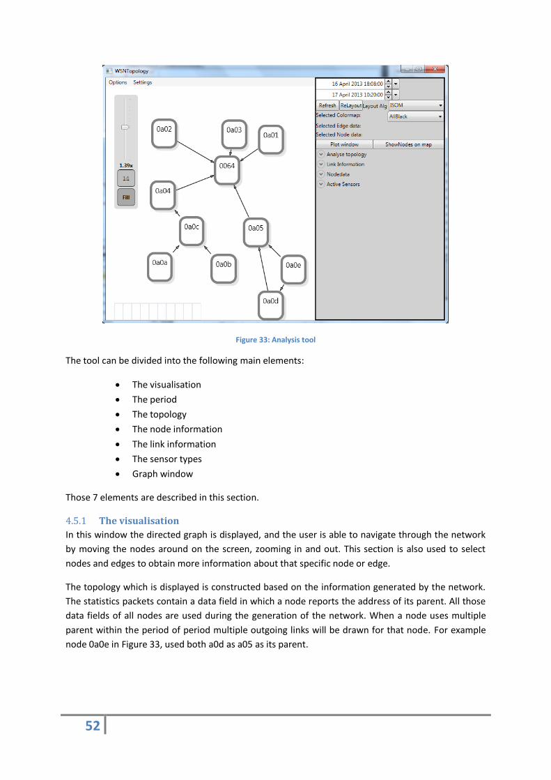
52
Figure 33: Analysis tool
The tool can be divided into the following main elements:
The visualisation
The period
The topology
The node information
The link information
The sensor types
Graph window
Those 7 elements are described in this section.
The visualisation 4.5.1
In this window the directed graph is displayed, and the user is able to navigate through the network
by moving the nodes around on the screen, zooming in and out. This section is also used to select
nodes and edges to obtain more information about that specific node or edge.
The topology which is displayed is constructed based on the information generated by the network.
The statistics packets contain a data field in which a node reports the address of its parent. All those
data fields of all nodes are used during the generation of the network. When a node uses multiple
parent within the period of period multiple outgoing links will be drawn for that node. For example
node 0a0e in Figure 33, used both a0d as a05 as its parent.

53
The period 4.5.2
To select the period a start and end time setter are used. The first one specifies the start time and
the second one the end time. This time is used to query the database and thus the analysis for the
network will be done based on the selected time period.
The topology 4.5.3
During the selected period the topology could change over time. This might result in a network
where nodes have several down links and the actually used topologies cannot be extracted from the
first summary of the by the network used topologies. It could be interesting to see what topology is
used at what time and how the topology develops over time.
Next to only visualizing the used topology at a certain time point only showing the most used link
from each node might give a better understanding of the network.
The menu to control this in illustrated in Figure 34.
Figure 34 Topology analysis interface
When looking at the deployment based on time there are two options to select a topology. The first
option is to step through the various used topologies by clicking on the next and previous. The way
the sequential development of the topology can be analysed. When a more specific time is of
interest the scroll bar can be used to scroll through time and select a specific time point.
This function should give the network engineer the opportunity to analyse a highly dynamic network.
It should help to see how the network changes over time, and what topology dynamics are occurring.
Using this function links of interest can be separated from those which are not important for the
network.
Node Information 4.5.4
The nodes send data to the sink for analysis. The information of each node is aggregated and
attached to node in the visualization. By selecting a node from the topology the information will be
displayed in this section. The information is divided into different boxes. Each tap will contain its own
type of information. The 4 taps are:
- Node QoS
- Node statistics
- Node sent packets counters
- Others
All statistics from can also be used to select any data type which should be displayed in the nodes in
the visualisation. This way the values of all nodes of a specific statistic can easily be compared. In
Figure 35 an example of the node data window is shown.

54
Figure 35: Node data window
Those four types are further discussed here.
4.5.4.1 Node QoS
The node QoS matches the given quality of service requirements with the measured behaviour of a
node. The user can predefine the required quality of service of each node. Then the tool will match
this requirement with the actual performance of the node and sees if the node is operating according
to those requirements. The only quality of service metric which is analysed at the moment is
reliability as described in 4.2.2.2 and added to that will the longest period of consecutive packet loss
be showed here. This however can later be extended when lifetime and latency analysis are made.
This metrics represents the amount of data that is received at the sink. Later when the network is
further developed this can be extended with for example lifetime and latency.
4.5.4.2 Node statistics
The node statistics give information about how the node is performing, and what it did in the period.
Information like the average packet reception ratio, number sensor/statistics packets sent and the
average ETX of the uplink are given in this. This list of information is a small summary of how active
the node was.
The metrics shown here are:
- Number of missed packets: the number of packets a node sent to the sink but did never
reach it.
- Number of used link: the number of different down links the node used
- Link ETX The average value of the downlink during the period
- Estimated link quality: the estimated link quality based on the ETX corrected for the
number of retransmissions used.
4.5.4.3 Node sent packets counter
The activity of a node can be analysed based on counters which are embedded in the statistics
packets. The number of for example sent sensor/statistics and routing packets are summarized in
this tap .
The statistics available in this tab are:

55
- Nr of packets sent, this is the number packets created by the node itself.
- Number of packets received, the number or routing and configuration packets received
by the node
- Nr of packet forwarded, this is the number of packets that are successfully sent to a node
and that it forwarded to its parent.
- Nr of data packets sent, this is the sum of sensor, statistics and routing packets is the
number of data packets sent by a node
- Number of sensor packets, this is the absolute and relative number of sensor packets a
node sent. The relative value is relative to the number of data packets sent.
- Number of statistics packets, this is the absolute and relative number of statistics packets
a node sent. The relative value is relative to the number of data packets sent.
- Router solicitation sent, this is the number of times a node requests other nodes their
network status. This is done when re-evaluating its parent.
- Router advertisements sent, this is the number of times a node responds to router
solicitations of other nodes
4.5.4.4 Others
When extra sensors are added for examination of the deployment, the average value and deviation
of the dataset can be found on this tab.
The link information 4.5.5
The edge information has the same purpose as the node information. It should give the user a
summary of the information available for the link. Just as on the node is the information on the link
also divided into multiple tabs. The available taps are:
- List statistics
- Link indicators
Just as with the node information can the all metrics in the different tabs be used to display on the
edges in the visualisation to compare the different values of all edges. Figure 36 shows an example of
the link information window.
Figure 36: Link information window

56
4.5.5.1 Link statistics:
The link statistics yield some basic numbers on of the link. This contains statistics like load, number of
packets over the link absolute and relative to the number of packets sent by the node or how many
packets a the node missed using that link.
The statics are:
- Estimated load in p/s.
In section 4.3.2 a method is described to determine the load in packets per second on
each link is described. This method is used to determine the load on each link
- Number of activations.
This number indicates how often the node switched to that specific link. And is given in
an absolute and relate to the total number of link changes number.
- Nr of missed packets.
An absolute and relative to the total number of transmitted packets number indicating
how many packets where lost on that link
- Number of packets over link.
An absolute and relative number indicating the number how many packets where
transmitted. The relative number shows how much per cent of packets where
transmitted over that link
4.5.5.2 Link indicators
The link indicators section contains the metrics that are used in section 4.1 to analyse the network.
The used values are:
- RSSI up average and deviation
- LQI up average and deviation
- RSSI down average and deviation
- LQI down average and deviation
- ETX average
- Link ETX average and deviation
- Estimated link quality based on the link ETX and configuration
The sensor types 4.5.6
Next to the analysis of the standard network indicators is can also all other types of sensors which
are on the nodes be added to the analysis. Sensors like for example the temperature can be selected
to be included in the analyses and then will the average and deviation be added to the The nodes
information. Also the graphs of those sensors can be plotted in the plot window. Figure 37 shows the
sensor selection window.

57
Figure 37: Sensor selection window
Graph window 4.5.7
All the previously described data are either absolute average or relative values over the complete period. This can give a good first understanding of the network. However to get real insight in the dynamics of the networks time graphs are important. These graphs can show the different links or nodes perform over time. To show these graphs a different window is created. This window is illustrated in Figure 38.
Figure 38: Plot window
This window contains 2 columns. The first one contains a list of all nodes and edges. When selecting
a node or edge all the available plots will be listed in the right window. By selecting a instance in both
columns the requested plot can be selected and added by the add button. So the dynamics of the
network can be further examined.
Conclusion 4.6The central question for this chapter was: Once a wireless sensor network is deployed what
information can be extracted from the active deployment for analysis, and can this information be
used to (re)configure the network?
This question could only partially be answered. Analysing the wireless sensor network can be done
based on the information the network supplies. However analysing a network involves more than
looking at just a single moment in time. Wireless sensor networks tend to have a dynamic behaviour
making it hard to analyse the network over time. Single links at certain moments are easy to analyse,
but analysis of the changing topology combined with variations in link quality is challenging.
When analysing the network this should be done in three layers. First the transport layer, this
analyses the connectivity of a node with the sink independent of its location in the network. Second
the link layer. This layer looks at the quality of the links used in the network based on the probability
that a packet is successfully transmitted over the link. And the third layer is the physical layer. This
layer checks the signal of each link which is used for communication.
In order to make the analysis of a network easier an analysis tool is developed. This tool visualises
the topology of the network. Within the visualisation, aggregations of all metrics which are sent by

58
the nodes to the sink can be visualised on the nodes or links. Next to the aggregations, the plots of
all metrics can be created; this makes analysing the network easier.
When the network is analysed the performance of the network is better known. This knowledge of
the performance is used to see if the network’s configuration can be derived from these analyses.
The relation between the metrics and the behaviour of the network is used to determine the
required configuration for the specified quality of service of the network.
In order to test the derived configurations a test setup was made using the Nimbus wireless sensor
network test bed. However this test bed was only tested in a single configuration setting and caused
failures in other configuration settings, like for example when the nodes where using different
transmission powers, the network is unable to operate in a normal way which caused the
configuration method to be untested.

59
5 Linking the Deployment to the Design The previous sections considered what information could be extracted from the network to evaluate
the performance of a network once deployed. This section will consider what can be taken from the
network and feed back to the design phase in order to support a system integrator when evaluating
changes in the deployment (i.e. node positions). As was stated previously the design can only provide
an estimate of connectivity however due to changes in the environment it is very difficult to know if
this is reflected in reality and if not then can it be improved from analysing the network connectivity.
For the initial design using the deployment tool the floor plans of a building are given as input and
used to estimate the propagation of the signals within the environment. This enables a user to design
without any physical measurements at a building offering a great advantage because now a design
can be made without visiting the building. The downside is that since only limited knowledge of the
building is used the quality of the design might not be sufficient for the application.
This section will focus on how the models used to predict the signal propagation and whether it can
be adjusted using the network data. This information can either be a site survey or the output from a
deployment. Both will contain data about the signal attenuation between a transmitter and receiver.
This data is than compared to the estimated values and the differences can be used to improve the
estimation model.
At the last week of my research information which was unknown to me raised. This information
would have led to other approaches to improve one of the models (ray tracing model). However due
to the late notice I was not able to process this new information and conduct a proper research using
this. Therefor the described method regarding the ray tracing model will probably not be
implemented, but since this thesis should also describe my work I left it in there.
Different models for signal estimations exist. The two most commonly used are the multi wall model
[23] [24] [25] and the ray tracing model [26] [27]. The ray tracing model is currently being used by
the design tool but it also can use an optimised version of the multi wall model after a detailed site
survey. For both models the theory and how they can be used to improve the predication quality for
the design tool will be explained.
The multi wall model: 5.1The multi wall model is an empirical model and used to predict the attenuation between a
transmitter and a received. The model contains 3 components of signal loss. [24]
Free space attenuation
Distance attenuation
Object attenuation
All those components will be described here.
Free space attenuation: 5.1.1
The free space attenuation, also called Pl(0) or path loss 0, is a static number of signal loss that is
caused by the gain of the transmitter, receiver and the frequency of the signal used for propagation.

60
By definition the free space attenuation component is given by the loss of signal at 1 meter from the
transmitter. The formula is given in Equation 19.
Equation 19: Free space loss multi wall model [25]
λ represents the wavelength of the used signal. The wavelength of the used 2.4 GHz signal is 0.12491
meter. Filling in this parameter in Equation 19 gives a free space loss of 40 dBm.
(
)
This means that the signal loss at one meter distance from the transmitter is 40.05 dBm. Thus the
best possible received signal power is 0 dBm maximum transmission power minus 40 dBm free space
attenuation, which equals -40 dBm.
Distance attenuation 5.1.2
The second component is the propagation distance attenuation. This number represents the amount
of signal that is lost between the transmitter and the receiver based on the distance between the
two. This factor can be determined by Equation 20.
(
)
Equation 20: Distance attenuation for the multi wall model
In this formula, d represents the distance between the receiver and the transmitter, d0 is the unit in
which the distance is measured and n the attenuation factor. This factor n should be tuned based on
measurements in the building. The structure of each building is different and the signal quality is
heavily influenced by the structure. Therefore this number can vary for each building.
To determine this value a site survey should be performed. A site survey means that at different
distances and different locations within the building the signal strength is measured. These
measurements are than used to determine the value for n.
Wall attenuation 5.1.3
The third component is the signal loss due to objects such as walls that intersect the direct path
between the transmitter and receiver. Walls and other object are harder to propagate through, and
should therefore be taken into account when estimating for the total loss factor. Those object types
will have a constant attenuation factor. To determine the attenuation of propagating through walls a
site survey just like for the distance factor is used.
The cost for propagating through walls can be determined at different levels. One cost factor that is
equal for all walls, or get a cost factor per wall type when a building has multiple wall types for
example, a heavy outside walls, glass walls or a lighter internal walls. To obtain a cost factor per wall
can lead to a higher accuracy in the model but this has as downside that the required dataset to tune
the costs for each wall should be much larger than to for the two other types. Thus it is a trade-off
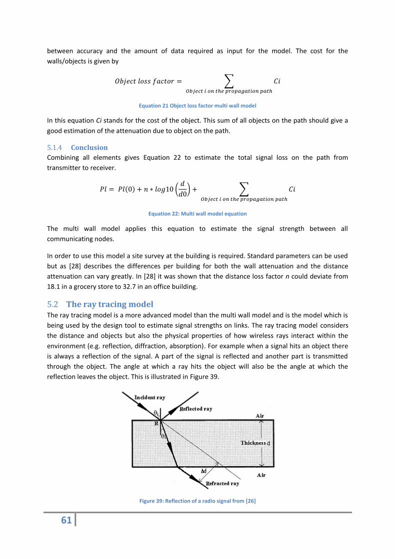
61
between accuracy and the amount of data required as input for the model. The cost for the
walls/objects is given by
∑
Equation 21 Object loss factor multi wall model
In this equation Ci stands for the cost of the object. This sum of all objects on the path should give a
good estimation of the attenuation due to object on the path.
Conclusion 5.1.4
Combining all elements gives Equation 22 to estimate the total signal loss on the path from
transmitter to receiver.
(
) ∑
Equation 22: Multi wall model equation
The multi wall model applies this equation to estimate the signal strength between all
communicating nodes.
In order to use this model a site survey at the building is required. Standard parameters can be used
but as [28] describes the differences per building for both the wall attenuation and the distance
attenuation can vary greatly. In [28] it was shown that the distance loss factor n could deviate from
18.1 in a grocery store to 32.7 in an office building.
The ray tracing model 5.2The ray tracing model is a more advanced model than the multi wall model and is the model which is
being used by the design tool to estimate signal strengths on links. The ray tracing model considers
the distance and objects but also the physical properties of how wireless rays interact within the
environment (e.g. reflection, diffraction, absorption). For example when a signal hits an object there
is always a reflection of the signal. A part of the signal is reflected and another part is transmitted
through the object. The angle at which a ray hits the object will also be the angle at which the
reflection leaves the object. This is illustrated in Figure 39.
Figure 39: Reflection of a radio signal from [26]
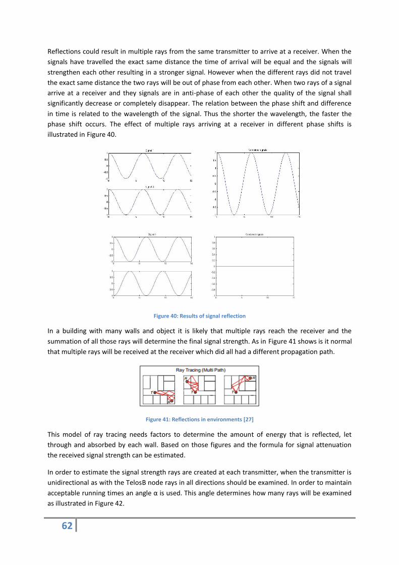
62
Reflections could result in multiple rays from the same transmitter to arrive at a receiver. When the
signals have travelled the exact same distance the time of arrival will be equal and the signals will
strengthen each other resulting in a stronger signal. However when the different rays did not travel
the exact same distance the two rays will be out of phase from each other. When two rays of a signal
arrive at a receiver and they signals are in anti-phase of each other the quality of the signal shall
significantly decrease or completely disappear. The relation between the phase shift and difference
in time is related to the wavelength of the signal. Thus the shorter the wavelength, the faster the
phase shift occurs. The effect of multiple rays arriving at a receiver in different phase shifts is
illustrated in Figure 40.
Figure 40: Results of signal reflection
In a building with many walls and object it is likely that multiple rays reach the receiver and the
summation of all those rays will determine the final signal strength. As in Figure 41 shows is it normal
that multiple rays will be received at the receiver which did all had a different propagation path.
Figure 41: Reflections in environments [27]
This model of ray tracing needs factors to determine the amount of energy that is reflected, let
through and absorbed by each wall. Based on those figures and the formula for signal attenuation
the received signal strength can be estimated.
In order to estimate the signal strength rays are created at each transmitter, when the transmitter is
unidirectional as with the TelosB node rays in all directions should be examined. In order to maintain
acceptable running times an angle α is used. This angle determines how many rays will be examined
as illustrated in Figure 42.

63
Figure 42: Ray creations
When setting α to a very small angle many rays are created and estimations of all reflections can be
calculated. However the smaller α, the more computation power is required. Thus a trade-off should
be made when setting alpha. In this case the model is used in a 2 dimensional fashion. In order to
further increase its accuracy the 3th dimension could be included. However this will lead to far more
complex system with way longer running times.
Analysis based on site survey data 5.3To evaluate the different models and the possibility for adjustments the data from a site survey that
was already carried out within the Nimbus Building by others. This site survey contains a big dataset
where the signal strength is measured throughout the building. The prediction quality is measured by
the mean absolute error and the mean squared error. The error is defined as the difference between
the estimated and measured value. The absolute mean error indicates the average error per sample,
and the mean squared error is an indicator which is used to give more weight to the outliers.
The site survey 5.3.1
The site survey consists out of 3 scenarios, illustrated in Figure 43, Figure 44 and Figure 45. Scenario
1 and 2 have 5 nodes and scenario 3 got 4 nodes. All nodes are located on the same floor of the
building. The site survey consists of the measurements between the nodes from a scenario and a
sixth node which is used to measure the node to node RSSI.
The data gathering was performed with an extra node this node will be moved around the building in
a constant phase. During the movement the signal strength values to the other nodes was measured
and stored. Afterwards the location of the node was added to the measured signal strengths based
on linear interpolation over time. When the path that the node took is known, and the speed at
which it is moved around the location of the node in each moment in time is known. Based on this
information the site survey is able to measure the RSSI over the entire building.
Figure 43: Scenario 1

64
Figure 44: Scenario 2
Figure 45: Scenario 3
On the floor plan of the building three different colours are used to draw the walls. Those different
colours represent different types of walls. The black lines are heavy walls, the green lines are light
walls and the grey lines are glass walls and windows. This results in a dataset of about 2000-2500
points per scenario.
In order to be able to benchmark the different techniques the three different scenarios of the site
survey are used. For each technique one of the scenarios will be used as input and then tested
against the complete set. In this way the learning set contains only one third of the test it is tested on
and should give a good indication on whether the method can estimate the signal strength outside its
own learning set. In the design tool only the ray tracing model is implemented. This implementation
will act as a baseline to compare all the results to. The results are given by Table 4.
Scenario Mean absolute error Mean square error
1 6.9 74.8
2 17.7 388.0
3 9.7 140.2
All scenarios combined 10.6 177.8 Table 4: Ray tracing model benchmark
On this site survey data set the average absolute error over the complete data set is 10.6 dBm. The
free space loss for the used frequency is 40 dBm and the least amount of measurable signal is -95
dBm. Thus the prediction space is from -40 to -95 dBm, which is a range of 55 dBm. On a range of 55
dBm is an average error of 10 dBm is relative high. However these estimations can be made with only
the floor plan of a building and no site surveys have to be conducted before the first analysis can be
made.

65
Analysis of Model Predictions 5.3.2
That data of the site survey will be used to test how the multi wall model and the design output
performs. And it will be seen if the models can be adjusted to see if the estimation quality can be
improved with the site survey data as learning data.
5.3.2.1 Analysis of the quality of the multi wall model
An implementation of the multi wall model was undertaken. In order to test the implementation only
one of the three scenarios from the site survey set is used to learn the parameters of the model so
that the model can then be tested on the complete dataset. For this method two different
implementations are made, one where all walls are considered the of the same type and will thus
have the same attenuation value, and one where each wall type (heavy walls, light walls and glass
walls) will have its own attenuation value.
To determine the attenuation factors for the distance and walls linear regression is used. Linear
regression is a mathematical technique which tries to fit a line through a set of points with the least
mean square error. This technique can also be used in a multi-dimensional set of points, like for
example multiple wall types. In that case multiple independent variables will get their own values.
Determining parameters of the model is done in two phases. In the first phase the parameter for the
distance loss factor is learnt for each scenario. After this the costs of the wall or walls types are
learnt. This is done because the distance loss attenuation is independent of the walls and should
therefore be determined first. Than based on this factor can the wall attenuation factors be
determined. When the distance and wall attenuation factors are determined together the distance
loss attenuation factor can be influenced by the errors from the wall attenuation factor.
For learning the distance loss attenuation factor all measurements where the signal does not
intersect a wall are used as the input. Based on this set the relation between the distance and the
signal loss has to be determined. In Figure 46 the scatter plot of all points where no walls are in
between the transmitter and receiver are scattered in blue. All those point where corrected with the
free space loss attenuation, since the goal is to find out what the loss is caused by the distance and
all other signal lost should be taken out of the measurements. Those points are the input for the
linear regression. The red line is the output. The linear regression formula finds the line that has the
best fit with a set of points.

66
Figure 46: Site survey scenario 1 learning the distance loss parameter multi wall model
As Figure 46 shows not all the input points lay on the red line. Each measurement will have a
deviation from the predicted signal. This deviation can come from either an inaccurate measurement
method or the model does not capture all attenuation sources, like for example fading. When the
deviation of the measurement method is evenly divided the use of more points will average out this
the error. Thus more points will improve the design quality.
After learning the attenuation factor for the distance the same technique is applied for the walls the
results are shown in Table 5.
Learning scenario
Distance loss factor
1 Wall type cost
3 wall types: Heavy light glass
1 -31.5637 -1.2417 -1.2736 -0.5828 0
2 -19.8664 -3.3066 -2.7828 -4.5129 -2.7597
3 -35.6873 -1.3994 -1.188 -1.8183 -2.838 Table 5: Multi wall model parameter learning
This table shows that the parameter the model learns heavily relies on the learning set. Even though
all used learning sets come from the same type of communicating nodes and the same building the
results are very different. For example the distance loss factor of scenario 3 is 79% bigger than in
scenario 2. This makes learning the parameters for the model hard, since it is difficult to know
whether the learning data is good or bad if there is no benchmarking. Therefore in general it can be
said that the more points the learning data contains the smaller the errors of the learnt parameters.
To be able to compare the results benchmarking is applied. For the benchmarking of the learned
parameters in the previous table are tested on the complete dataset from the site survey. The results
of this benchmark are shown in Table 6
Single wall Multi wall model Three wall types multi wall model
Learning Scenario Mean abs error Mean square error
Mean abs error Mean square error
1 5.4 49.2 5.5 50.6
2 9.8 132.9 9.4 123.8
3 6.4 65.7 6.4 64.9 Table 6: Multi wall model benchmarking

67
When comparing the results of all scenarios it becomes clear this model is performing better than
the ray tracing model for this specific configuration which had a mean absolute error on the
complete dataset of 10.6 and a mean square error of 177.8. This is somewhat expected as it is tuned
specifically to the environment where the prediction is carried out and it is not fair to directly
compare both models rather to show that the multi wall model can be accurately tuned to reflect a
very specific configuration but may not easily adapt to the general case.
5.3.2.2 Adjusting the ray tracing model with site survey information.
The ray tracing model initially estimates signal strengths between a transmitter and a receiver purely
based on the floor plan of the building. The error from the model can be reduced by a number of
possible options, 1. Improve the environment description, 2. Characterise the hardware better
(radiation pattern, orientation etc) or 3. Optimise the parameters of the walls for the specific types
based on site survey data. For the context of this research access to the model implementation is not
available. As a result it was investigated if a simple offset could be generated based on the data
collected within the network to create a closer fit between the prediction and measurement.
Just like with the parameter learning of the Multi Wall Model linear regression is used to find the
adjustment values for the propagation distance and the different wall types. The difference between
this approach and the multi wall model is that here adjustments are made on top of an already
existing modes. The differences between the estimation’s and the measured values are used as
input.
The learned parameters for the ray tracing model are shown in Table 7.
Learning scenario
Distance loss factor
Single wall type
Multiple walls types
Heavy wall Light wall Glass wall
1 -2.5 2.1 2.3 2.5 -1.8
2 2.7 2.8 2.9 2.1 3.4
3 -7.8 4.2 4.3 3.3 6.6 Table 7: Correction coefficients for the Ray tracing model
Even though these parameters adjust the same model and the learning scenarios come from the
same building the outcome of the parameters are completely different. The used datasets did all
contain more than 2000 samples to learn the parameters but still the differences are high.
To see what the effects of the learnt coefficients are will the results be tested on the complete
dataset. The results of the adapted ray tracing model are given in Table 8.
Learning scenario Single wall type Multiple wall types
Mean absolute error Mean square error
Mean absolute error
Mean square error
1 8.0 104.2 8.0 103.5
2 8.0 98.1 7.9 96.2
3 8.4 111.5 8.4 111.5 Table 8: Error values of the adapted ray tracing model
The error rates of all three scenarios are significantly lower than without the wall correction,
therefore can be concluded that correcting the ray tracing model based on measurements in the

68
building will increase the estimation quality of the signal strength even though the outcomes can be
very different.
In Figure 47: Scenario 3 model adjustment using a single wall the result of the adjusted model is plot
together with the original estimation and the measured value. The figure was created using scenario
3 to lean the parameters and one wall was considered. This figure shows that the adjusted ray
tracing model is able to more accurately estimate the signal strength than the original model.
Figure 47: Scenario 3 model adjustment using a single wall
In Figure 48 the difference in the estimated value between the ray tracing model and the adjusted
ray tracing model is plotted. This shows that for most of the samples the adjusted ray tracing model
had a better prediction than the original ray tracing model. There are multiple samples where
estimations of th adjusted model are worse. Due to those samples with decreased quality can be
concluded that this method is not monotonically decreasing. This makes the use of it harder since it
can’t be proven that the adjustments to the model will lead to better results in each specific case.
The average over a large dataset will give a better result which indicates that the adjustments are
improving the model.
Figure 48: Difference in estimation error between adjusted model and original model
Now that the ray tracing model and the multi wall model both had learned their parameters from a
site survey data set both models can be compared. This comparison shows that the multi wall model
is still performing better than the Ray tracing model, thus when a site survey is constructed it is
better to use the multi wall model than the adjusted ray tracing model.
Ray tracing model adjustment based on the data from real 5.4
deployments When a deployment is deployed which does not fulfil its requirements redeployment has to be
considered. However the initial design created using the design tool did not estimate the reality
sufficient enough to come to good quality design. Therefore the estimation should be improved
based on the information given by the real deployment. Thus the design tool should be able to learn
based on the information from the deployment.
From the analysis of the site survey it is possible that using real data can improve both the multi wall
model and the ray tracing model. However these analyses require relative large data sets where
available. Each site survey scenario contained over 2000 samples. These big datasets are normally

69
not available and only the information which is can be extraction from a real deployment can be
used.
When a deployment is used of for example 10 to 20 nodes normally no more than 30 samples are
known. This data set is too small to successfully learn the parameters of the multi wall model.
Therefore only corrections for the ray tracing model are considered.
When learning from site survey data sets two different leaning methods where used. One was to
consider all walls of the same type, and the other one to create different parameters for the different
types of walls. The differences between the results of two different methods were small. In some
cases the method where only 1 wall was used performed even better than the method where three
different wall types where considered and the other way around. Overall the two methods
performed more of less the same. Therefore only wall type is considered in this section. The more
parameters need to be learned the bigger the dataset should be, since the used dataset is very small
the number of learning parameters should be kept to a minimum.
Ray tracing model update using a single wall type 5.4.1
The input for the updating the model is the data which comes from a real deployment. The used
deployment and the by the deployment tool estimated RSSI values is illustrated in Figure 49. The
deployment contains 10 nodes and a sink. The deployment used during operation 11 different links.
That means that the dataset available for the model adjustments also contain 11 point.
Figure 49: Deployment used for updating ray tracing model

70
First the distance attenuation factor is adjusted. Since the deployment contained only 4 links which
did not propagate through walls the data set for this is really small. Figure 50 shows the 4 points and
the fitted line. This set resulted in a distance adjustment factor of -2.9.
Figure 50: Distance versus prediction error
Figure 51: Parameter learning based on real deployment data
As Figure 51 shows does this learning set have a relationship between the number of walls the signal
propagates through and error in the model. The red line shows the relationship which is learned

71
based on this input dataset. A same relation exists for the distance however, due to the limited input
where only 4 samples known to learn the distance adjustment factor.
This relationship is that for each wall a correction of 3.9 should be applied to the estimation.
Testing this on the dataset which is obtained by the site survey shows that the mean average is now
8.3 instead of 10.6 and the mean square error 114.1 instead of 177.8. This is a significant decrease of
the mean absolute error by about 20% and the for the mean square error the decrease is even
stronger. This shows that on average the prediction quality is increased and that there is a decrease
of outliers.
From this can be concluded that using a small learning set can already give a significant improvement
of the quality of the ray tracing model, and is therefore advised to use when redeployments are
considered.
Ray tracing model update where each wall is wall has its own correction value 5.4.2
Next to the optimisation where all walls are considered to have the same error rate another option
to update the model exists. Since the difference between each prediction and measurement is
known local optimisation is also possible. In this case all walls considered too be independent
objects, thus the correction factors are no longer related. Instead the prediction error will be evenly
divided by all walls which are in-between the transmitter and receiver. This way the prediction is
adjusted in such a way that for that specific case all predictions match. However in the prediction not
all the errors come only from the walls. Also errors are introduced by the distance signal loss
estimation. This error is in the first case added to the walls.
When redeployment is considered nodes will be relocated or new nodes are added to the network.
The correction values for the walls contain the combined errors of the walls and the distance signal
loss error. Thus the estimated values for the relocated or added nodes are likely to be incorrect.
However since the error of the distance is assumed to be smaller than the error for the walls the
remaining error is assumed to be smaller than the initial error. When multiple values for a single wall
exists the error for the distance loss is likely to be filtered out and in this way only the error for each
specific wall will remain.
Applying this method to the deployment used for this section and tested on the site survey data
gives a mean absolute error of 10.3 and a mean squared error of 167. These results are slightly better
than the original 10.6 and 177.8 but the change is only small. Therefore I suggest that this is not the
model to use.
Conclusion 5.5The goal of this section was to find out how to improve the quality of a deployment. To do so the
model used for predictions of the signal strengths are analysed. For those analysis a benchmark was
setup. This benchmark is used to see what the quality of the model is and how any changes to model
improve or degrade the quality of the estimations.

72
For improving the design two different approaches where used. One is to use a relative large data set
obtained by a site survey to adapt the model. The other approach is to only use the data from an
deployment.
When a site survey set is present two different models can be used to estimate signal strengths
through the building. A simple Multi Wall Model, or the more advanced ray tracing model. The multi
wall model estimates the signal strength based on the distance between a transmitter and receiver
and the number and types of walls on the propagation path. The ray tracing model includes next to
the distance and wall types also reflections. When a signal hits a wall a part of the signal is reflected.
This reflection can have a great impact on the signal strength.
From the dataset adjustment parameters for the walls should be extracted. The ray tracing model
already estimates the cost of propagating a signal through a wall, the goal of learning is to improve
the estimated cost of the walls. This can be done by estimated the cost per wall type. A heavy wall is
likely to absorb more signal than a light wall and should thus get another cost value. However
comparing the cost per wall approach with having a single wall type and thus a single cost the results
are almost the same. Therefor I would suggest to use single wall types when doing these model
adjustments.
From the analysis of the site survey learning approach did the multi wall model show the best results
with an average mean absolute error of 7.2dBm where the original model had and mean absolute
error of 10.6dBm. The improved ray tracing model gave an average mean absolute error of 7.7 dBm.
The results of the ray tracing model and the multi wall model are almost the same however, the
multi wall model got a lot deviation in its results, in 3 samples it had as the best result of 5,4 dBm and
the worst of 9,8 dBm. The ray tracing model seems more stable where the best result was 7,3 dBm
and the worst 8,3 dBm. Therefor I would recommend to use the ray tracing model when improving a
model based on a site survey dataset.
Next to the site survey dataset also the possibilities of improving the signal strength estimation based
on the data from an active deployment is analysed. The mayor difference between the learning from
an active deployment and from a site survey is size of the dataset. A indoor deployment typically
exists out of 10 to 50 nodes. From a deployment of this size can 50 to 150 links be used as input for
adapting the model. With the site survey 2000 points where used to learn the model.
Due to the small dataset which can be used when the data is extracted from active deployments can
only the ray tracing model be used. Since this model does not have to learn all its parameters from
the dataset but only creates adjustments to the model. From earlier analysis we already saw that
assuming that all walls are of the same type will give just as good results as using multiple wall types.
Adjusting the ray tracing model based on an small deployment of 11 nodes and tested the results on
the site survey data gave as result that the mean absolute error went from 10.6 dBm to 8.2. This is an
22% improvement. Therefore can be concluded that even though the datasets which can be
extracted from small deployment the original model can be adjusted to significantly improve the
design quality.
Next to adjusting the ray tracing model using a single wall type it is also possible to give each wall a
correction value. This way local optimizations can be made. When an estimation contains an error,

73
this error can be adjusted by changing to cost value of the walls on the propagation path. This
method leads to local optimizations. However the estimation error is not only induced by the walls
on the propagation path. So when adjusting only the walls cost value all other errors will be included
in this value. When moving node, the other errors like distance loss will change while it is still
encapsulated in the cost value for the wall. When repeating this multiple times, the other errors will
filter out and a cost value per wall remains. This method is not very useful when using it on the data
set from a real deployment since this method will required multiple measurements per wall, and this
data set will often only contain a single value per wall.
Overall can be concluded that adapting the ray tracing model and learning the multi wall model
based on the data from a site survey both will give a significant improvement over the results of the
original ray tracing model. However for this method a site survey is required. When no site survey is
performed and only the data form a deployment is known the data set to lean the adjustment
parameters from is small. Therefor only the ray tracing method will be adjusted. The quality of the
model using the only the small dataset is also improved, but not as much as when the site survey is
conducted. Therefor is suggest that only the single wall method is used when adjusting the ray
tracing model based on the data from a deployment.
74
6 Conclusion This thesis focused on the following objectives:
1. What data can be extracted from a live network and how can it be used to analyse and verify
the performance of the WSN post-deployment?
2. How can the network be configured/re-configured in the case of poor performance to ensure
requirements are met while maintaining a maximum lifetime?
3. How can the extracted information be feed back to the design phase to improve on the site
specific deployment?
After the planning and deployment of a wireless sensor network is done the question arises. “How
well does the network perform, and is the current configuration the optimal configuration of the
network?” In order to be able to answer those questions the first objective is used. What data can be
extracted from a live network and how can it be used to analyse and verify the performance of the
WSN post-deployment?
Analysing a wireless network is done at three different abstraction layers. The physical layer, which
checks the quality of the signal used for communication, the link layer which checks the probability a
packet is transmitted successfully between two nodes and the transport layer which checks the
connectivity of a node with the sink. Each layer has its own related metrics and its own way of
analysing the network. This is discussed extensively in section 4.1. What this section shows is that for
all 3 layers metrics exist in the network which reflect the quality of the layer. For the physical level
the RSSI values show that as long as the RSSI is over -87 dBm that the physical link will be of a good
quality. As soon as the RSSI value drops below the -87 dBm the link quality will degrade rapidly. For
the link-layer quality the ETX metric is used. This number is the inverse of the probability that a
communication over both the up and down links succeeds. This number can be used to estimate the
probability that a packet is successfully transmitted over the down link. The last metric used for the
analysis is the packet reception ratio. This number reflects the ratio between number of packets that
reached the sink and that where created by each node. Multiple methods are available to estimate
the end-to-end packet reception rate. Testing those methods showed that using EWMA was the
method that showed the strongest relation.
Once analysis can be made the configuration of the network is the next concern. Is the network
configured in such a way that it utilises its resources as good as possible. Or “How can the network
be configured/re-configured to ensure requirements are met while maintaining a maximum lifetime?”
In this thesis a configuration framework was created. The configuration framework strives to create a
configuration that meets the by the application required quality of service while maintaining a
maximum lifetime of the network. The lifetime is optimized by minimizing the load on the entire
network. To do so 3 configuration options are used. The transmission power of the nodes, the
maximum number of retransmissions and the number of duplications of the packets.
The transmission power is configured independently of the number of retransmissions and number
of duplications. As the analysis of the RSSI showed, the link maintain a high quality when the RSSI
values are higher than -85. When the worst incoming or outgoing link from a node is 7 or 15 dBm
higher, -85, the transmission power of that node can be lowered without compromising on the
quality of the communication.

75
The number of duplications and number of retransmissions are configured based on the ETX values
of the links. The ETX reflects the communication quality of a link and is therefore used to estimate
the reliability of the nodes. Retransmissions on a link level or duplicating packets on a node level will
both impact the reliability of a node at the same way. However when retransmissions are used all
packets that are forwarded by that node will be retransmitted which might lead to an unnessery
induced extra load on that node. When not all nodes require the same reliability the nodes that have
a higher reliability might compensate the bad network quality by sending multiple instances of the
same packet, so that no retransmissions on a link level are required. To determine what the best
configuration are, two formulas are used to calculate the total load on the network. By finding the
configuration that delivers all nodes their required QoS and minimizing the load on the network the
optimal configuration can be found.
This method will create a configuration for the network based on the information from a specific
point in time. To do so the topology and the link qualities are used as input. However one the
property of wireless sensor networks is that they are highly dynamic. Thus the used topology and the
link quality could vary over time, making the derived configuration invalid. In order to maintain a
good network the configuration should be updated continuously.
To verify the configuration framework the Nimbus test bed was used. This test bed was tested under
one specific configuration. Using other configurations caused the network to be unstable or to be
unable to from a network at all. Due to these problems, I was unable to verify the configuration
framework. Therefore no statements about the quality of the configuration framework can be made.
The other part of thesis focused on how information from deployments can be used to improve the
deployment planning. This involved the question: “How can the extracted information be feed back
to the design phase to improve on the site specific deployment?” To answer the question two
estimations models where used. The already implemented ray tracing model and the multi wall
model. The results of those two models are compared to each other. For improving the quality of the
models two different inputs were used. Ones from a site survey, which contains a relative large data
set, and one is from a deployment which contains a small dataset. To measure the quality of a model
the by the deployment tool used ray tracing model and the site survey data set was used. This data
set contained over 7000 points. The mean absolute error and the mean square error over the site
survey data set where taken as a benchmark. The mean absolute error was 10.6 dBm and the mean
square error 177.8.
First the site survey; the complete site survey consists of 3 scenarios. Each scenario alone was taken
as input to improve the model. The result was then tested against the complete site survey dataset.
The results show that even though the datasets are al relatively large and gathered in the same
building with the same nodes the differences outcome of the different scenarios are large. Even
though the outcomes might differ all outcomes were better in estimating the attenuation than the
original ray tracing model.
Comparing the results of the two different models shows that the Multi wall model is on average
better able to estimate the signal strengths than the ray tracing model. However the ray tracing
model is more constant and therefore I would recommend to use the ray tracing model.

76
The second scenario was improving the estimation quality based on the data from real deployments.
A test deployment was used that contained 11 links. Thus the input set was 11 points large. Due to
the limited size of the input set is only the ray tracing model was taken into account. Learning the
adjustment parameters and comparing to the benchmark shows that even though the input set was
small the adjustments to the model did significantly improve the estimation quality. The mean
absolute error was reduced by 22% and the mean square error by 36%. This means that not only the
average prediction quality is much better but also that the adjusted model contains significantly less
outliers. This means that the probability of an estimation of specific points if more likely to reflect the
actual value than before.
This theses suggested a method for configuring the network. However this method was not
extensively tested. Therefore the next step should be to update the test bed, and use the suggested
configurations to see how it works. Another issue which needs to be solved in the future is how to
cope with the dynamics of the network in relation to the configuration. How long is a configuration
valid, and thus how often should the network be recon figured?
Once the configuration methodology is tested and it turns out to be working fine, a next step would
be so research how this can be done in a distributed way. Now everything is done in a centralized
fashion which is possible for small networks, but when the network size increases to hundreds of
nodes this would not be feasible and distributed QoS support should be the next step to tackle this
problem.
77
7 Bibliography
[1] D. Hui and R. Han, “A node-centric load balancing algorithm for wireless sensor networks,”
Global Telecommunications Conference, pp. 548-552, 2003.
[2] M. Nabi, M. Geilen and T. Basten, “An Empirical Study of Link Quality Estimation Techniques for
Disconnection Detection in WBANs”.
[3] S. Dawson-Haggerty, A. Tavakoli and D. Culler, “Hydro: A Hybrid Routing Protocol for Low-Power
and Lossy Networks,” Smart Grid Communications (SmartGridComm), vol. Oct, pp. 268-273,
2010.
[4] S. Poduri, S. Pattem, B. Krishnamachari and G. Sukhatme, “Sensor network configuration and the
curse of dimensionality,” IEEE Workshop on Embedded Networked Sensors, May 2006..
[5] X. Cheng, D.-Z. Du, L. Wank, B. Xu and D, “Relay sensor placement in wireless sensor networks,”
ACM/Springer Journal of Wireless Networks, vol. 14, p. 347 355, 2008.
[6] W. Wei, C. Wan-Dong, W. Bei-Zhan, W. Ya-Ping and T. Guang-Li, “The Factor Graph Approach for
Inferring Link Loss in MANET,” International ocnference on Internet computing in science and
engineering, 2008.
[7] K. Srinivasan and P. Levis, “RSSI is Under Appreciated,” In Proceedings of the Third Workshop on
Embedded Networked Sensors, 2006.
[8] V. Erceg, L. J. Greenstein and S. Y. Tjandra, “An Empirically Based Path Loss Model for Wireless
Channels in Suburban Environments,” IEEE JOURNAL ON SELECTED AREAS IN
COMMUNICATIONS, vol. 17, pp. 1205-1211, 1999.
[9] A. Mainwaring, D. Culler, J. Polastre, R. Szewczyk and J. Anderson, “Wireless sensor networks for
habitat monitoring,” ACM international workshop on Wireless sensor networks and applications,
pp. 88-97, 2002.
[10] D. Hughes, P. Greenwood, G. Blair, G. Coulson and P. Grace, “An experiment with reflective
middleware to support grid-based flood monitoring,” Concurrency and Computation: Practice &
Experience , pp. 1303-1316, 2006.
[11] G. Coulson, R. Gold, M. Lad, C. Mascolo and L. Mottola, “Dynamic Reconfiguration in the RUNES
Middleware,” Mobile Adhoc and Sensor Systems (MASS), pp. 574-577, 2006.
[12] N. Vlajic and D. Stevanovic, “Performance Analysis of ZigBee-Based Wireless Sensor Networks
with Path-Constrained Mobile Sink(s),” Sensor Technologies and Applications, pp. 61-68, 2009.
[13] P. Radmand, A. Talevski, S. Petersen and S. Carlsen, “Comparison of industrial WSN standards,”

78
Digital Ecosystems and Technologies (DEST), pp. 632-637, 2010 .
[14] C.-K. Brendan , G. David , E. Desmond and S. C. Ricardo , “Performance evaluation of the
6LoWPAN protocol on MICAz and TelosB motes,” Performance monitoring and measurement of
heterogeneous wireless and wired networks, pp. 25-30, 2009.
[15] . A.-E.-B. Mostafa, A. M. Y. Mohamed and M. A.-O. Mariam , “WIRELESS SENSOR NETWORKS –
PART I: TOPOLOGY AND DESIGN ISSUES,” Electrical and Computer Engineering, pp. 1165-1168,
2005.
[16] E. Stavrou and A. Pitsillides, “A survey on secure multipath routing protocols in WSNs,”
Computer Networks, vol. 54, no. 13, pp. 2215-2238, 2010.
[17] S. K. Singh, M. P. Singh and D. K. Singh, “Routing Protocols in Wireless Sensor Networks – A
Survey,” International Journal of Computer Science & Engineering Survey (IJCSES), vol. 1, no. 2,
pp. 63-83, 2010.
[18] Crossbow, “Crossbow TelosB Datasheet,” Crossbow.
[19] Chipcon, Datasheet of the CC2420 radio chip used in the telosB nodes.
[20] N. Javaid, A. Javaid, I. Khan and K. Djouani, “Performance study of ETX based wireless routing
metrics,” Computer, Control and Communication, pp. 1-7, 2009.
[21] Y. Wei , J. Heidemann and D. Estrin, “Medium Access Control With Coordinated Adaptive
Sleeping for Wireless Sensor Networks,” Networking, IEEE/ACM Transactions on, vol. 12, no. 3,
pp. 493-506, 2004.
[22] C. Chee-Yee and S. Kumar, “Sensor networks: evolution, opportunities, and challenges,”
Proceedings of the IEEE, no. 91, pp. 1247-1256, 2003.
[23] L. Ruiz, J. Nogueira and A. Loureiro, “MANNA: a management architecture for wireless sensor
networks,” Communications Magazine, IEEE , no. Feb 2003, pp. 116-125, 2003.
[24] D. Chen and P. K. Varshney, “QoS Support in Wireless Sensor Networks: A Survey,” Conference
on Wireless Networks.
[25] S. Hadim and N. Mohamed, “Middleware: middleware challenges and approaches for wireless
sensor networks,” Distributed Systems Online, pp. 1-23, 2006.
[26] M. Perillo and W. Heinzelman , “Providing Application QoS through Intelligent Sensor
Management,” Sensor Network Protocols and Applications, pp. 93-101, 2003.
[27] L. Chenyang , B. Blum, T. Abdelzaher, J. Abdelzaher and H. Tian , “RAP: a real-time
communication architecture for large-scale wireless sensor networks,” Real-Time and Embedded
Technology and Applications Symposium, pp. 55-66, 2002.

79
[28] T. Rappaport and S. Sandhu, “Radio-wave propagation for emerging wireless personal-
communication systems,” Antennas and Propagation Magazine, pp. 14-24, 1994.
[29] M. Lott and I. Forkel, “A multi-wall-and-floor model for indoor radio propagation,” Vehicular
Technology Conference, pp. 464 - 468, 2001.
[30] J. Zhong , L. Bin-Hong, W. Hao-Xing, C. Hsing-Yi and T. Sarkar, “"Efficient ray-tracing methods for
propagation prediction for indoor wireless communications,” Antennas and Propagation
Magazine, pp. 41 - 49, 2001.
[31] G. Wahl, P. Wölfle and P. Wertz, “Dominant Path Prediction Model for Urban Scenarios,” Mobile
and Wireless Communications Summit, p. ?, 2005.
[32] S. Seidel and T. Rappaport, “914 MHz path loss prediction models for indoor wireless
communications in multifloored buildings,” Antennas and Propagation, pp. 207-217, 1992.
[33] A. Guinard, “A Design Tool for WSN Design in Buildings,” Mater Thesis at Nimbus. 2011