Snorre Kvemdokk

Depletion of Fossil Fuels andthe Impacts of Global Warming

AbstractThis paper combines the theory of optimal extraction of exhaustible resources with the theory ofgreenhouse externalities, to analyse problems of global warming when the supply side is considered. Theoptimal carbon tax will initially rise but eventually fall when the externality is positively related to the stockof carbon in the atmosphere. lt is shown that the tax will start falling before the stock of carbon in theatmosphere reaches its maximum. If, on the other hand, the greenhouse externality depends on the rate ofchange in the atmospheric stock of carbon, the evolution of the optimal carbon tax is more complex. It caneven be optimal to subsidise carbon emissions to avoid future rapid changes in the stock of carbon, andtherefore future damages. If the externality is related to the stock of carbon in the atmosphere and thereexists a non-polluting backstop technology, it will be optimal to extract and consume fossil fuels even whenthe price of fossil fuels is equal to the price of the backstop. The total extraction is the same as when theexternality is ignored, but in the presence of the greenhouse effect, it will be optimal to slow the extractionand spread it over a longer period.

Keywords: Global warming, exhaustible resources, carbon taxes, backstop technology

JEL classification: D62, Q38

Acknowledgement I am indebted to Michael Hoel for helping me structuring the ideas and for hiscomments, to Kjell Arne Brekke for valuable discussion and comments, and to Knut Alfsen, SamuelFankhauser, Petter Frenger and Rolf Golombek for comments on an earlier draft. I am also grateful to AtleSeierstad for helpful discussion. This paper was financed by Norges forskningsråd (Økonomi og Økologi),and is a part of Metodeprogrammet at Statistics Norway.

1. Introduction

One main environmental challenge in our time is to avoid or reduce the impacts of global

warming. Carbon dioxide (CO2) is the main greenhouse gas, and 70-75% of all CO2

emissions is due to combustion of fossil fuels (see for example Halvorsen et al. (1989)). In

most papers analysing the economics of global warming, the supply of fossil fuels is

modelled like any other good, and the exhaustibility of these resources is not considered.

There have been many studies on externalities from fossil fuel consumption and the depletion

of exhaustible resources (see, e.g., Dasgupta and Heal (1979), Baumol and Oates (1988) and

Pearce and Turner (1990)), but few authors have tried to combine these two theories. Among

the first studies is Sinclair (1992) who analyses the impacts on consumer and producer prices

of a constant tax rate on energy use besides the development of a carbon tax. He argues that

in steady state, the ad valorem carbon tax should be falling over time. This is followed up in

Ulph and Ulph (1992). The authors study the evolution of an optimal carbon tax using

quadratic benefit and damage functions. They find that the carbon tax (in both specific and

ad valorem terms) should initially rise but eventually fall. Sinclair's conclusion, they argue, is

driven by very odd assumptions. Devarajan and Weiner (1991) use a two-period model to

analyse the importance of international global warming agreements, assuming that the

consumption of fossil fuels in period two is the difference between the initial stock of fossil

fuels and period one consumption. Finally, Withagen (1993) compares the optimal rate of

fossil fuel depletion without greenhouse externality with the case where this externality is

present.

In this paper I combine the theory of greenhouse externalities with the theory of exhaustible

resources using the framework of a simple model described in section 2. The first problem

analysed is the design of the optimal policy response. Most studies analysing the damage

from global warming, specify the damage as a function of the temperature level or

alternatively the atmospheric concentration of greenhouse gases (GHGs). However, because

the ecology can adapt to a certain change in the climate, given that the rate of change is not

too high, it can be argued that what matters is the speed of climate change (e.g., the rate of

change in temperature or atmospheric concentration) and not only the level of temperature

itself. This argument is taken seriously by national governments, in the way that they have

3

committed themselves to annual emissions restrictions of GHGs. 1 Thus, in section 3 the

optimal carbon tax is derived and compared for two different specifications of the damage

function; one in which the damage is due to the level of global warming, and the other where

damage is related to the speed of climate change.

The optimal policy response is analysed without considering possible substitutes for fossil

fuels. Even today there exist several alternatives to fossil fuels, however at higher costs. The

traditional result from the theory of a competitive mining industry facing a backstop

technology with a constant unit cost of extraction less than the choke price, is that the

industry will deplete the resource until the price reaches the cost of the backstop. At this

price, the resource is exhausted, and the consumers will switch immediately to the backstop.

Introducing external greenhouse effects, will, however, give some new results described in

section 4. I summarise the conclusions in section 5.

One example is the Norwegian Government which aims at stabilising the annual CO, emissions on 1989 level by2000.

4

2. The Model

This section describes the basic model of the paper. I assume that the social planner

maximises the present value of welfare to the global society given a competitive market of

fossil fuels. That is, he seeks an extraction path of fossil fuels which will

ISO

maximise 5 e -11 -[u(x,) —c(A,)x,—D(S,)]dt

(1)

where x is the extraction (and consumption) of all fossil fuels in carbon units, u(x) is the

benefit of the society from fossil fuels consumption, c(A)x is the extraction cost, A, = Ix tdt

is accumulated extraction up to time t, S is the atmospheric stock of carbon in excess of the

preindustrial stock and D(S) expresses the negative externality of carbon consumption. r > 0

is a discount rate and to > 0 represents the depreciation of carbon in the atmosphere. These

parameters are fixed throughout the analysis. Further I set Ao = O and So > O.

The benefits from fossil fuel consumption are assumed to increase in current consumption

(ul(x) > 0), but the marginal utility is bounded above (u'(0) < co) and decreasing (u"(x) <

0 and u 1 (00) = 0). Define u(x) = p(x)dx, where p(x) is the consumer price. The utility

function, u(x), is therefore similar to the consumer surplus, and the marginal utility equals

the consumer price (u'(x) = p).

The total extraction cost, c(A)x, increases both with the current extraction rate (c(A) > 0 for

all A) and the cumulative extraction up to date (c'(A)x > 0 for x > 0). Furthermore, the

marginal extraction cost is constant, and I assume c"(A)x > 0 for x > O. This means that

the incremental cost due to cumulative extraction rises with the amount already extracted. No

fixed quantity is assumed for the total availability of the resource. However, in line with

Farzin (1992), only a limited total amount will be economically recoverable at any time. This

is due to the assumption c"(A)x > 0 for x > 0, which means that increasingly large

quantities of the fossil fuel resource can be exploited only at increasingly higher incremental

5

costs. With c(A) — 00 as A — 00, it will be optimal to extract a finite amount of the resource

since the marginal utility is bounded above. Thus, on the optimal path, the cumulative

extraction reaches an upper limit, A, as t 00. This gives limit_ c(A)x = 0, i.e., c(Ã) < 00.

The damage from global warming is a function of the atmospheric stock of carbon.' I have

not taken into account the lags between the atmospheric stock of carbon and the climate, a

lagged adjustment process which is due to the thermal inertia of oceans (see Houghton et al.

(1990, 1992)). The stock is increasing in fossil fuel combustion, but decays with the

depreciation rate ô > 0, according to the atmospheric lifetime of CO2 . This is of course a

simplification. The depreciation rate is probably not constant, but will decrease with time

since a possible saturation of the carbon-sink capacity of the oceans as they get warmer, will

give a longer lifetime of CO2 in the atmosphere (see Houghton et al. (1990, 1992)).

However, I stick to this assumption for the time being, since it is widely employed in

economic studies of global warming, see, e.g., Nordhaus (1991, 1993), Peck and Teisberg

(1992), Ulph and Ulph (1992) and Withagen (1993). The preindustrial stock is assumed to be

an equilibrium stock, meaning that the atmospheric stock will approach the preindustrial level

in the long run (S 0) when fossil fuels are exhausted. I assume that the damage can be

described by an increasing and convex function of the atmospheric stock (i.e., D'(S) > 0 and

D"(S) > 0 for all S > 0), but that they are negligible for the initial stock increase (D'(0) =

0). There is no irreversible damage which means that D(S) 0 as S O.

From the model, we find the consumer price as the sum of the producer price and a carbon

tax, v (see Appendix A). The producer price is the sum of the marginal extraction cost, c(A),

and the scarcity rent N. Thus, introducing a carbon tax separates the consumer price and the

producer price.

(2) p, = c(A,) + + vi

In Appendix A, it is shown that the extracted amount of fossil fuels will fall over time in the

absence of the externality (D(S) = 0 V S). With a constant carbon tax, v, the total extracted

amount of fossil fuels will go down, but if the tax approaches zero in the long run (v 0),

the accumulated extraction equals total extraction in the absence of a carbon tax.

2 Alternatively we could specify the damage as a function of the temperature level. However, I simplify the matterssince the temperature is positively related to the atmospheric stock of carbon (see Houghton et al. (1990, 1992)).

6

3. The Optimal Policy Response to Global Warming

Most studies analysing the damage from global warming assume that the damage is related to

the temperature level (see, e.g, Nordhaus (1991, 1993), Peck and Teisberg (1992) and

Kvemdokk (1994)). However, it can be argued that the damage will depend as much on the

rate of temperature change as on the absolute value itself, because the ecology is able to

adapt to a certain temperature change. There are however costs of adapting to a new stage

(see for instance Tahvonen (1993)). If the rate of climate change is high, there may be a

period of large damage until the original species have been replaced by more resistant ones.

Agriculture is a sector highly dependent on the change in temperature. Another example is

human beings, who are capable of adjusting to climatic variations, and can live under more

or less every climatic condition existing on earth. However, rapid changes in climate have

impacts on human amenity, morbidity and mortality (see Fankhauser (1992) and Cline

(1992)). As the optimal policy response to global warming may depend on how we specify

the damages, it is important to study the optimal carbon tax under the different specifications

of the damage function. The damage from global warming probably depends on both the

level of the climate as well as the rate of climate change. Therefore, damage functions taking

into account only one of these elements must of course be considered as extreme cases.

Analysing the two elements separately, however, points out some main features.

3.1 Damage Related to the Atmospheric Stock of Carbon

Consider first the case where damage is related to the atmospheric stock of carbon, as

modelled in section 2. The optimisation problem is solved in Appendix B. The optimal

solution can be implemented by a carbon tax (8 0) representing the discounted future

negative externalities due to accumulation of carbon in the atmosphere.

.0

(3) 0 1 = fe -(r415)(1--t) D (5' v) dt

The optimal carbon tax has the following properties (see Appendix B), where 6 is the time

derivative of the tax:

7

(4) lim,, 13, = 0

OS

(5) 6, = fe" )(" ) D "(ST)-gtdt

(6) hal t_ 6 1 =o

From (3) we see that the carbon tax is positive as long as marginal damage is positive, that is

as long as S > O. It will smoothly approach zero in the long run as the stock of carbon in the

atmosphere decays and reaches the equilibrium stock (see (4) and (6)). This means that the

tax will be positive even if the atmospheric stock declines after a certain time due to low

extraction and consumption of fossil fuels; the decay of carbon in the atmosphere is higher

than the additional carbon from new extraction (x < 8S).

Figure 1: The Optimal Carbon Tax when Damage is Related to the Atmospheric Stock ofCarbon

a=b

é t = e -(r. "— " D"(s r )-štdt

8

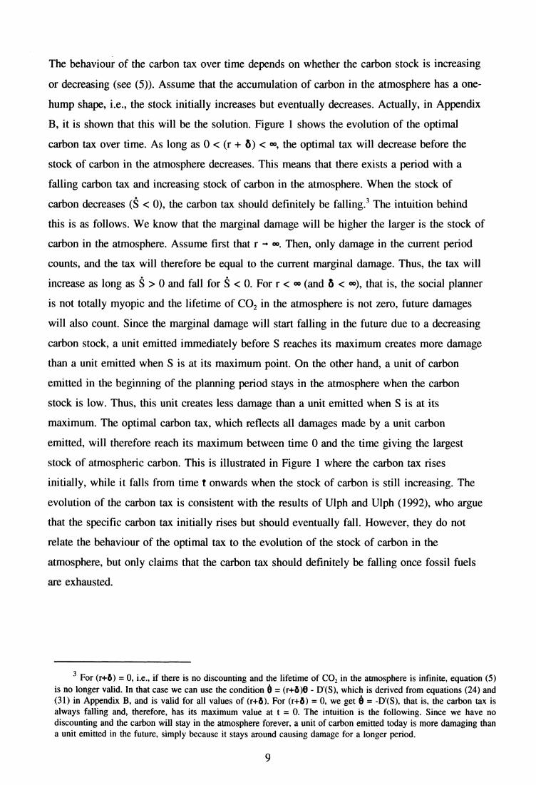
The behaviour of the carbon tax over time depends on whether the carbon stock is increasing

or decreasing (see (5)). Assume that the accumulation of carbon in the atmosphere has a one-

hump shape, i.e., the stock initially increases but eventually decreases. Actually, in Appendix

B, it is shown that this will be the solution. Figure 1 shows the evolution of the optimal

carbon tax over time. As long as 0 < (r + 8) < 00, the optimal tax will decrease before the

stock of carbon in the atmosphere decreases. This means that there exists a period with a

falling carbon tax and increasing stock of carbon in the atmosphere. When the stock of

carbon decreases < 0), the carbon tax should definitely be falling. 3 The intuition behind

this is as follows. We know that the marginal damage will be higher the larger is the stock of

carbon in the atmosphere. Assume first that r 00. Then, only damage in the current period

counts, and the tax will therefore be equal to the current marginal damage. Thus, the tax will

increase as long as Š > 0 and fall for Š < O. For r < 00 (and ô < 00), that is, the social planner

is not totally myopic and the lifetime of CO2 in the atmosphere is not zero, future damages

will also count. Since the marginal damage will start falling in the future due to a decreasing

carbon stock, a unit emitted immediately before S reaches its maximum creates more damage

than a unit emitted when S is at its maximum point. On the other hand, a unit of carbon

emitted in the beginning of the planning period stays in the atmosphere when the carbon

stock is low. Thus, this unit creates less damage than a unit emitted when S is at its

maximum. The optimal carbon tax, which reflects all damages made by a unit carbon

emitted, will therefore reach its maximum between time 0 and the time giving the largest

stock of atmospheric carbon. This is illustrated in Figure 1 where the carbon tax rises

initially, while it falls from time t onwards when the stock of carbon is still increasing. The

evolution of the carbon tax is consistent with the results of Ulph and Ulph (1992), who argue

that the specific carbon tax initially rises but should eventually fall. However, they do not

relate the behaviour of the optimal tax to the evolution of the stock of carbon in the

atmosphere, but only claims that the carbon tax should definitely be falling once fossil fuels

are exhausted.

3 For (r-1-6) = 0, i.e., if there is no discounting and the lifetime of CO2 in the atmosphere is infinite, equation (5)is no longer valid. In that case we can use the condition ô = (r+6)I3 - D'(S), which is derived from equations (24) and(31) in Appendix B, and is valid for all values of (r+6). For (1+6) = 0, we get 6 = -1Y(S), that is, the carbon tax isalways falling and, therefore, has its maximum value at t = O. The intuition is the following. Since we have nodiscounting and the carbon will stay in the atmosphere forever, a unit of carbon emitted today is more damaging thana unit emitted in the future, simply because it stays around causing damage for a longer period.

9

3.2 Damage Related to the Rate of Change in the Atmospheric Stockof Carbon

As argued above, another alternative is to model the negative externality as a function of the

time derivative and not the level of the atmospheric stock. Some first attempts in this

direction have been made by Tahvonen (1993), Tahvonen et al. (1994) and Hoel and Isaksen

(1993). These papers, however, do not take into account the exhaustibility of fossil fuels.

It is reasonable to believe that there are costs of adapting to a colder (§ < 0) as well as a

warmer climate (§ > 0), and that these costs increase the higher is the rate of climate change.

Therefore, I assume that the damage is convex in the rate of atmospheric carbon

accumulation. Further, there are no damage costs for a constant climate (§ = 0). Hence, if

d(£) is the damage function, we have d(Š) > 0 for Š 4 0, and d(0) = O. I also assume that the

damages are negligible for marginal changes in the stock under a constant climate (§ = 0),

giving d'(0) = O. The convexity of damages means:4

(7) cli(g) > 0 for S' > 0 A d i(g) < 0 for S' < 0

d"(Š) > 0 for all g'

The new optimisation problem is thus:

00

maximise e "1"' -[u(x ,Adt

(8)

4 Alternatively, we could argue that small changes in the climate do not make any damage. This can be specifiedas d() = 4:1 1 ( 1 ) = 0 for IS I s K, where K is a constant. If K 6S, for all t, the decline in the atmosphericconcentration of CO, will never be large enough to make d'(Š) negative (as IŠ I = I6S I s K for x = 0). This willsimplify some of the results below, since in this case, the shadow price of the atmospheric stock, y, will always be non-negative (see (10)). However, for g > K, we will still have the two contradictory effects described below (see (9)). Inparagraph 3.1 above, we could in a similar way argue that D(S) = Di(S) = 0 for S s M, where M is a constant. Thiswould not change the main results, however, the carbon tax would reach zero in finite time when S, M for all t.

10

This model is solved in Appendix C where it is shown that the optimal carbon tax, a, can be

expressed as:

(9) = d"(Š,) - y,

where Tt is the shadow price associated with accumulated atmospheric stock up to t.

OD

(10) y, = 8 .fe -0-4) (T-o d /0,:d d,,

Consider first the situation with an increasing stock of carbon in the atmosphere (Š > 0).

Fossil fuel consumption (and extraction) increases the damage from global warming via

accelerated buildup of the atmospheric stock (represented by C•) in equation (9)), but on

the other hand, this leads to a larger stock in the atmosphere and therefore higher decay in

the future. A high decay will reduce the rate of change in the atmospheric stock, and hence

the damage from global warming. Note therefore, that while the shadow price of accumulated

atmospheric stock is negative in the first model where damage is determined by the stock

level (II = -8 < 0; see Appendix B), it is positive in the second model (y > 0) if Š > 0 for a

sufficiently long period.' This is also shown in Tahvonen (1993). Thus, a larger stock of

carbon in the atmosphere represents a cost if the damage is positively related to the level of

this stock, while it represents a benefit if the damage is positively related to the rate of

change in the stock as long as this stock is increasing for a sufficiently long period.

For Š < 0, an increase in fossil fuel consumption (and extraction) will reduce the absolute

value of Š, I Š I, and therefore the adaption costs. This effect gives a lower optimal carbon

tax, and is represented by CŠ) < 0 in (9). However, increasing fossil fuel consumption

gives a larger stock of carbon in the atmosphere, and therefore a larger decay of this stock in

the future. This leads to even lower values of Š, and higher adaption costs, in the future.

Thus, while the shadow price of accumulated atmospheric stock may be positive for Š > 0, it

is negative when Š < O.

5 Typically, the stock of carbon in the atmosphere will initially increase but eventually decrease (see AppendicesA and B). Therefore, the shadow price associated with accumulated atmospheric stock, y, consists of both positive andnegative elements as WO > 0 for S > 0 and WO < 0 for S < 0 (see equation (10)). This means that S has to bepositive for a sufficiently long period for y to be positive.

11

Increasing fossil fuel consumption may therefore give two contradictory effects. From (9) we

see that the carbon tax can be negative or positive depending on which effect is the strongest.

This is also a different result compared to the model expressed in (1), where the optimal

carbon tax is always non-negative.

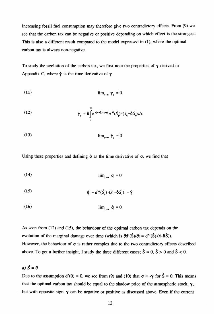
To study the evolution of the carbon tax, we first note the properties of y derived in

Appendix C, where t is the time derivative of y

(11) lim,œ y, =

IS

(12) = 8 f e -(r+6)(1.1) d"(Š)-(1,-8.5')dt

(13) lim, t, = 0

Using these properties and defining IT as the time derivative of a, we find that

As seen from (12) and (15), the behaviour of the optimal carbon tax depends on the

evolution of the marginal damage over time (which is äd'(Š)/ät = d"(Š).(i-)).

However, the behaviour of a is rather complex due to the two contradictory effects described

above. To get a further insight, I study the three different cases; Š = 0 Š > O and Š < O.

a) hg = 0

Due to the assumption CO) = 0, we see from (9) and (10) that a = -y for Š = O. This means

that the optimal carbon tax should be equal to the shadow price of the atmospheric stock, y,

but with opposite sign. y can be negative or positive as discussed above. Even if the current

12

emissions make no change in the current atmospheric stock and therefore give no current

damage, it will be optimal to increase the emissions if the future atmospheric stock is

increasing for a sufficiently long period of time. Increased emissions will give a higher future

decay and reduce future damage. In this case it will therefore be optimal to subsidise

emissions. If the future stock is decreasing, we get the opposite conclusion.

b) Š > 0

If Š > 0 for a sufficiently long period of time, we see from (9) and (10) that a is positive if

and only if

(17) d"(Š) > y,

which means that the direct effect of an increase in the atmospheric stock of carbon is larger

than the indirect effect of increased future decay of this stock. However, even if the optimal

tax is positive, it is difficult to say anything about its evolution. From (15) we see that the

condition for a rising carbon tax is

(18) d ll(Š,)-(i t -agt ) - t t > 0

c) Š < 0

For Š < 0, an increase in extraction means reduced adaption costs (C.) < 0). This goes in

the direction of a lower carbon tax. On the other hand, increasing extraction means larger

stock and therefore higher decay in the future leading to higher adaption costs (y < 0). Thus,

the optimal tax should be positive if the second effect dominates the first, i.e.,

(19)

Id 1(Š,)1 < I Y, I

Actually, for d' (.) < 0 and y < 0, this gives condition (17). The condition for an increasing

carbon tax is again given by (18).

For a decline in the atmospheric stock of carbon, it can therefore be optimal to have a

positive carbon tax. This confirms the result derived from model (1), but while the result in

13

that model rests on the assumption that stock levels larger than the initial stock give an

external effect, the result in model (8) is due to the assumption of positive adaption costs

even for reductions in the stock.

Figure 2: Possible Optimal Carbon Tax Paths when Damage is Related to the Rate ofChange in the Atmospheric Stock of Carbon

In Figure 2, some possible time paths for the optimal carbon tax are illustrated. The

behaviour of the optimal carbon tax in this model is more complex than in model (1). If So

were equal to zero, initially the tax would be positive since we move from a situation with

no external effects to a situation with external effects. This would then reflect the

preindustrial situation. However, as So > 0, the optimal carbon tax can be negative as well as

positive in the beginning of the planning horizon. The discount rate, r, and the lifetime of

CO2 (reflected in 8) are important for the evolution of the optimal carbon tax. If the discount

rate is high, and the lifetime of CO2 is long (8 is low), the future indirect effects may be

negligible. In that case, the optimal carbon tax is positive for Š > 0, while it is negative for Š

< O. In the long run, the carbon tax will steadily approach zero (see (14) and (16)).

14

In both models, the optimal carbon tax will approach zero as time goes to infinity, see (4)

and (14). As shown in Appendix A, this means that the optimal extraction will approach zero

as time goes to infinity. It is also shown that even if the damage from global warming is

specified differently, the total extraction is the same.

15

4. Optimal Depletion with a Non-polluting BackstopTechnology

So far, I have not explicitly considered the existence of substitutes for fossil fuels. However,

substitutes such as synthetic fuels, nuclear power, hydro power, biomass, solar and wind

power already exist. Assume that there exists a non-polluting perfect substitute for fossil

fuels, y, with an unlimited stock and a constant unit cost, E. In a competitive market, the

price will be equal to this cost since there are no stock constraints. By definition, a backstop

source is available in unlimited quantities at a constant marginal cost. The traditional result

from the theory of a competitive mining industry facing a backstop technology with the

constant unit cost less than the choke price, but higher than the initial marginal extraction

cost, is that the industry depletes the resource until the price reaches the cost of the backstop.

At this price, the consumers will switch immediately to the backstop (see Appendix D). This

result is also derived in for example Dasgupta and Heal (1979), but they assume a fixed

quantity of the exhaustible resource. The extraction path will be different in the presence of

external greenhouse effects. By introducing the non-polluting backstop into the model from

section 2, the social planner seeks to

maximise e ' -[u(x +y 1 ) -c(A 1 )x 1 -ty , -D(S ,)]dt

s.t. if, = x,

(20) Š t = x, -6 S

X I0

y 0

c(0) < E < u 1(0)

The necessary conditions for an interior optimum are given in Appendix D.

In accordance with section 2, I define u(z) = Ip(z)dz, z = x+y, where p(z) is the consumer

price. Then, u'(x+y) = p. In Appendix D, it is shown that on the optimal path, the consumer

price has to satisfy the following conditions:

16

p(x,+y,) = c(A,) + 7 + 8, , x, > 0

+y,) = E, y, > 0

As the negative externality is a function of the atmospheric stock of carbon, the optimal

carbon tax, (3, has the characteristics derived in paragraph 3.1. In Appendix A, I show the

properties of the scarcity rent, N. Note that the evolution of this rent is given by:

(23) a(c(A i )

at

Taking time derivatives of (21) and (22), and using (23), we find the evolution of the

consumer price:

(24) 13, r75 6„ x, > 0

(25) /3, =0, y, > 0

For c(0) < C, the consumer price will initially be lower than the price of the backstop. This

gives x > 0 and y = 0 since p < E. In other words, only fossil fuels will be consumed

initially. In the absence of a backstop, the consumer price would increase and approach u'(0)

since p = u'(x). But since 'd < u'(0), the price will at some time reach E. At this price, we

can have x > 0 and y > 0 at the same time (see (23) and (24)). The condition for this is:

(26) 1 =

that is, the optimal tax is falling with the same rate as the producer price is increasing,

namely the discount rate times the scarcity rent.

17

If the extraction of fossil fuels is so high that the consumer price rises above the price of the

backstop, it will not be optimal to consume fossil fuels due to the cheaper substitute. But if

we stop depleting fossil fuels when p = E, the stock of carbon in the atmosphere will

decrease = -8S < 0), and the optimal carbon tax will fall (see (5)). This means that the

consumer price of fossil fuels will fall below ë, which again makes fossil fuels economically

viable. Therefore, it will not be optimal to stop the extraction of fossil fuels. The optimal

extraction path of fossil fuels when p = ë is determined by:

(27) C = c(A t) + + 0,

When the consumer price of fossil fuels equals the unit cost of the backstop, it will be

optimal to consume both fossil fuels and the backstop. Fossil fuels will be extracted so that

the consumer price remains constant and equal to this unit cost.

The optimal consumer price path is illustrated in Figure 3a. The consumer price of fossil

fuels is constant and equal to the consumer price of the backstop technology (which is the

unit cost) from time ta onwards (see Figure 3a).

18

Figure 3: Optimal Extraction and Consumer Prices with a Backstop Technology

A)P Å

,

, .t a 1 tb

g.IMEM

C

...%..

'

.. ..

B)

ta tb

= With externalities

= Without externalities•• . . .• • • .• . .. ■■• •• • . •• •• . ..

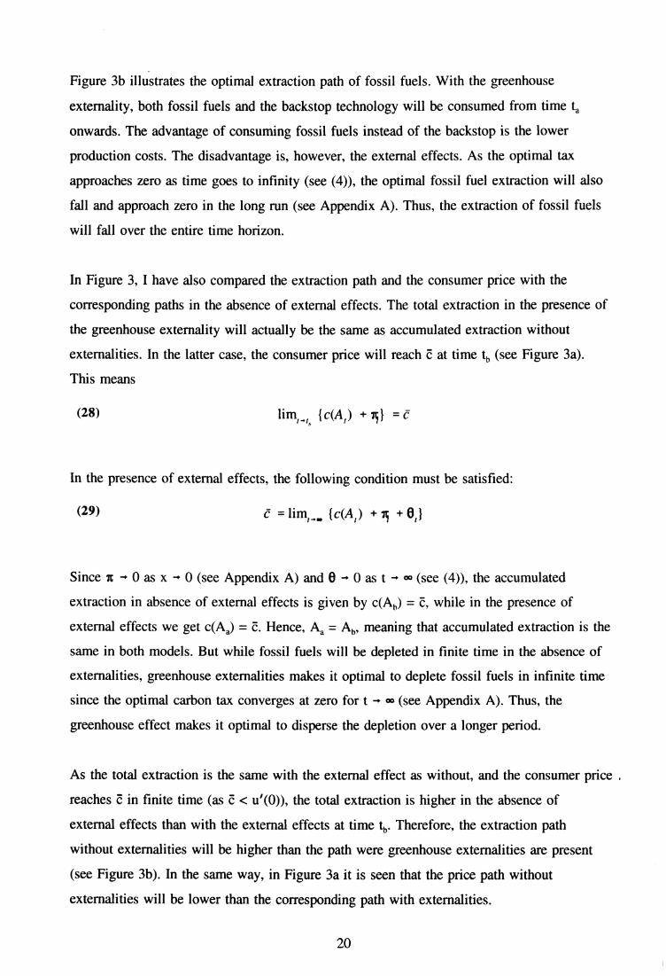
Figure 3b illustrates the optimal extraction path of fossil fuels. With the greenhouse

externality, both fossil fuels and the backstop technology will be consumed from time ta

onwards. The advantage of consuming fossil fuels instead of the backstop is the lower

production costs. The disadvantage is, however, the external effects. As the optimal tax

approaches zero as time goes to infinity (see (4)), the optimal fossil fuel extraction will also

fall and approach zero in the long run (see Appendix A). Thus, the extraction of fossil fuels

will fall over the entire time horizon.

In Figure 3, I have also compared the extraction path and the consumer price with the

corresponding paths in the absence of external effects. The total extraction in the presence of

the greenhouse externality will actually be the same as accumulated extraction without

externalities. In the latter case, the consumer price will reach sô" at time tb (see Figure 3a).

This means

(28) lim,1 {c(k) +} =

In the presence of external effects, the following condition must be satisfied:

(29) = {c(A) + ej

Since n — 0 as x 0 (see Appendix A) and #3 0 as t 00 (see (4)), the accumulated

extraction in absence of external effects is given by c(Ab) = E, while in the presence of

external effects we get c(Aa) = . Hence, Aa = Ab, meaning that accumulated extraction is the

same in both models. But while fossil fuels will be depleted in finite time in the absence of

externalities, greenhouse externalities makes it optimal to deplete fossil fuels in infinite time

since the optimal carbon tax converges at zero for t 00 (see Appendix A). Thus, the

greenhouse effect makes it optimal to disperse the depletion over a longer period.

As the total extraction is the same with the external effect as without, and the consumer price

reaches "d in finite time (as ë < u'(0)), the total extraction is higher in the absence of

external effects than with the external effects at time tb . Therefore, the extraction path

without externalities will be higher than the path were greenhouse externalities are present

(see Figure 3b). In the same way, in Figure 3a it is seen that the price path without

externalities will be lower than the corresponding path with externalities.

20

5. Conclusions

Most papers on the economics of global warming concentrate on the external effects from

fossil fuels combustion without taking into account the exhaustibility of these resources. This

paper combines the theories of greenhouse externalities and non-renewable resources, to

analyse several aspects of global warming.

The basic model presented in section 2, defines the negative greenhouse externalities as

positively related to the stock of carbon in the atmosphere. The exhaustibility of fossil fuels

is modelled by increasing extraction costs in accumulated extraction. A carbon tax is used to

implement the optimal solution to this model. This tax should initially be increasing but

eventually fall and approach zero as time goes to infinity. It should start decreasing before

the stock of carbon in the atmosphere reaches its maximum point.

Changing the specification of the externalities to depend on the rate of change in the

atmospheric stock of carbon, completely changes the model. While the shadow price of the

atmospheric stock was negative in the basic model, indicating a cost of increasing the stock,

it is positive in this new model if the stock of carbon rises over a sufficiently long period.

This is due to an increase in the depreciation of carbon in the atmosphere when the stock of

carbon increases, which gives a lower rate of change in the future stock. Actually, this effect

can make the optimal carbon tax negative even for high concentrations of carbon in the

atmosphere.

The last problem analysed is the depletion of fossil fuels if there exists a non-polluting

backstop technology. If we ignore the external effects, the traditional theory gives the result

that the resource should be depleted until the price reaches the cost of the backstop. At this

price, consumers will switch immediately to the backstop. Taking into account the

greenhouse effect will give different time paths for prices and extraction. When the consumer

price of fossil fuels reaches the price of the backstop, it will still be optimal with fossil fuel

consumption, that is, both the backstop and fossil fuels will be consumed. This is due to a

falling carbon tax of fossil fuels, and therefore a fall in the consumer price if fossil fuels are

not consumed. Total extraction will be the same as for no external effects, but the green-

house effect makes it optimal to slow down the extraction and spread it over a longer period.

21

References

Baumol, W. J. and W. Oates (1988): The Theory of Environmental Policy. Cambridge:Cambridge University Press.

Cline, W. R. (1992): The Economics of Global Warming. Washington, DC: Institute forInternational Economics.

Dasgupta, P. S. and G. M. Heal (1979): Economic Theory and Exhaustible Resources.Cambridge: Cambridge Economic Handbooks, Cambridge University Press.

Devarajan, S. and R. J. Weiner (1991): "Are International Agreements to Regulate GlobalWarming Necessary?", mimeo.

Fankhauser, S. (1992): "Global Warming Damage Costs: Some Monetary Estimates", GECWorking Paper 92-29, Centre for Social and Economic Research on the Global Environment(CSERGE), University College London and University of East Anglia.

Farzin, Y. H. (1992): "The Time Path of Scarcity Rent in The Theory of ExhaustibleResources", in: The Economic Journal, 102, 813-830.

Halvorsen, B., S. Kverndokk and A. Torvanger (1989): "Global, Regional and NationalCarbon Dioxide Emissions 1949-86 - Documentation of a LOTUS Database", Working Paper59/89, Centre for Applied Research, Oslo.

Hoel, M. and I. Isaksen (1993): "The Environmental Costs of Greenhouse Gas Emissions",mimeo, Department of Economics, University of Oslo.

Houghton, J. T., G. J. Jenkins and J. Ephraums (eds.) (1990): Climate Change - The IPCCScientific Assessment, (Report from Working Group I, The Intergovernmental Panel onClimate Change). WMO, UNEP, IPCC. Cambridge: Cambridge University Press.

Houghton, J. T., B. A. Callander and S. K. Varney (eds.) (1992): Climate Change 1992 - TheSupplementary Report to the IPCC Scientific Assessment, (Report from Working Group I,The Intergovernmental Panel on Climate Change). WMO, UNEP, IPCC. Cambridge:Cambridge University Press.

Kvemdokk, S. (1994): "Coalitions and Side Payments in International CO 2 Treaties",forthcoming in: E. C. van lerland (ed.), International Environmental Economics, Theoriesand Applications for Climate Change, Acidification and International Trade. Amsterdam:Elsevier Science Publishers.

Nordhaus, W.D. (1991): "To Slow or not to Slow: the Economics of the Greenhouse Effect",in: The Economic Journal, 101(407): 920-937.

Nordhaus, W.D. (1993): "Rolling the 'DICE': An Optimal Transition Path for ControllingGreenhouse Gases", in: Resources and Energy Economics, 15: 27-50.

Pearce, D.W. and R.K. Turner (1990): Economics of Natural Resources and the Environment.London: Harvester Wheatsheaf.

22

Peck, S.C. and T.J. Teisberg (1992): "CETA: A Model for Carbon Emissions TrajectoryAssessment", in: The Energy Journal, 13(1): 55-77.

Seierstad, A. and K. Sydsæter (1987): Optimal Control Theory with Economic Applications.Amsterdam: Elsevier Science Publishers.

Sinclair, P. (1992): "High does Nothing and Rising is Worse: Carbon Taxes Should be KeptDeclining to Cut Harmful Emissions", in: Manchester School, 60: 41-52.

Tahvonen, O. (1993): "Optimal Emission Abatement when Damage Depends on The Rate ofPollution Accumulation", in Proceedings of the Environmental Economics Conference atUlvön, June 10-13.

Tahvonen, O., H. von Storch and J. von Storch (1994): "Atmospheric CO 2 Accumulation andProblems in Dynamically Efficient Emission Abatement", forthcoming in: G. Boero and Z.A. Silberston (eds.), Environmental Economics. London: Macmillan.

Ulph, A. and D. Ulph (1992): "The Optimal Time Path of a Carbon Tax", mimeo, Universityof Southampton.

Withagen, C. (1993): "Pollution and Exhaustibility of Fossil Fuels", paper presented at the4th annual EAERE conference in Fontainebleau, June 30-July 3.

23

Appendix6

A. The Competitive Equilibrium when there is an Arbitrary Tax onFossil Fuels

Let v, be an arbitrary tax on fossil fuels at time t (measured in carbon units). The optimal

consumption/extraction path under a competitive equilibrium is then derived from the

maximisation problem below:

maximise e -[u(xd-c(Adx,-v txpt

(1)s.t. A, =x,

x 0

The existence of an optimal solution can be shown as follows. Assume c(0) > 0 and u'(00) =

O. It is easily seen that it never pays to have u'(x) - c(0) < 0 anywhere along a path, since

decreasing x on such intervals would then increase the integrand in the criterion, not only on

this interval but from then on and to infinity. Hence u'(x) - c(0) O. Choose a such that

u'(30 - c(0) < O. Then we can safely argue that x E [WI], and in fact that no optimal x, )1.

By Theorem 15, chapter 3, in Seierstad and Sydsæter (1987), an optimal control exists. This

proof is also valid for the model presented in Appendix B.

The current value Hamiltonian for problem (1):

(2) H = u(x) - c(A 1 )x, - v +

The necessary conditions for an interior optimum:

(3) aH =u (x) - c(A 1 ) -v 1 +A, s 0, (=0 for x 1 > 0)

6 The symbols and the concavity/convexity characteristics of the functions are explained in the main text.

24

(4) - rA _aH . cf(A)x,at,

A, =x 1

e 11 1 1 A 1 = 0

Due to the assumption u'(0) < co, we know that on the optimal path A, will converge (see

section 2), i.e.,

(7) 0 < 1im11, A, = À <

Therefore, from (6) and (7) we get:

(8) limtœ e = 0

A, (< 0) is the shadow cost associated with cumulative extraction up to t. Thus, the scarcity

rent at time t, x t, is defined as

(9)

To show the characteristics of the scarcity rent, I first use (4) and (8) to derive A t, thereafter

use (9) to find:

00

(10) = 5e ll"c (A ,)x icbc

limt_. =hint_ fe'c I(A.)x,chl e

applying L'Hepital's rule and notifying that by (7) x t 0 as t we get:

25

(12) = lim c 1(A

")x

= 0

According to (12), the scarcity rent will converge at zero for t 00. This is due to the

increasing marginal extraction cost; The costs will be so high that an additional unit of fossil

fuels extracted will not add to the welfare.

To find the optimal extraction path, consider (3). For x, > 0, this condition is fulfilled with

equality. Then, applying u 1 (x 1) = p, (see section 2), we find:

(13) p, = c(A,) +v,, x i > 0

Thus, the consumer price is separated from the producer price via the carbon tax. Further, the

producer price is the sum of marginal extraction costs and the scarcity rent, i.e., c(A) + 7C t .

The behaviour of the consumer price over time is given by

(14) = C "(A 1 )x, + i + , x, > 0

using (4), (9) and 15, = u"(x,),Z„ we find

(15) =u ll(x,).,C, = r75 +1,, x1 > 0

a) Assume v, = = 0 for all t. Since it > 0 for x, > 0 (see (10)) and u"(x,) < 0, we see that

< O. Thus, in the absence of a carbon tax the extraction of fossil fuels is falling and the

consumer price is rising over time.

b) Assume > O. Thus, we see from (15) that i < 0 as long as x, > O. Hence, with an

increasing carbon tax, the extraction of fossil fuels is falling and the consumer price is rising

over time.

26

c) Assume if, < O. We see from (15) that k < 0 as long as x, > 0 if and only if

(16)

Hence, with a falling carbon tax, the extraction of fossil fuels may rise and the consumer

price may fall over a limited period of time. Since accumulated extraction of fossil fuels will

converge, extraction of fossil fuels cannot increase forever.

As Š = x, - 6S„ initially Š > 0 if x > esSo. But eventually Š < 0 as x, decreases and S t

increases over time. In the long run S 0 since x, 0 when t 00. Hence, if .i, 0 for V t,

the atmospheric stock of carbon will initially increase but eventually decrease if S0 is not too

high.

As A — À, the extraction will fall and reach or converge at zero. If x, converges at zero in

infinite time, we have x, > 0 for all t, and equation (3) is fulfilled with equality. Assume x,

0 as t where I = min { t: x, = 0} < 00, and consider the case where we have no carbon

tax. By taking limit of (3) as t I, and using it = 0 (since x, = 0 for t uf, see equation

(10)), we find,

(17) u "(0) s c(À), x, =0

However, (17) has to be fulfilled with equality (see also the proof for an optimal solution

above). If not, the last unit of fossil fuels extracted and consumed reduces the welfare since

it gives a higher marginal cost (c(À)) than marginal utility (u'(0)). Thus, À is determined by:

(18) u "(0) = c(ii)

With constant v > 0, and by taking the limit of (3) as t 00, we get

(19) u "(0) = c(A) + v

27

By the same argument as above, (19) is fulfilled with equality. Thus, we see that with a

constant carbon tax, accumulated extraction of fossil fuels is less than without a carbon tax,

i.e., A < À.

If vt 0 as t 00, and by taking the limit of (3) as t cc, we are back to (18). Thus, if the

carbon tax approaches zero in the long run, the accumulated extraction of fossil fuels equals

the extraction in the absence of a carbon tax. However, as long as vt decreases, the producer

price has to increase, giving a positive extraction of fossil fuels. This is seen from equation

(15), which is fulfilled with equality according to the argument above. Hence, it will never

be optimal to stop depleting as long as the carbon tax is falling.

B. Damage as a Function of the Atmospheric Stock

Assume that there is a negative externality related to the atmospheric stock of carbon. If the

social planner seeks to maximise the present value of the welfare to the society, we get the

following optimisation problem:

4.11

maximise fe' lu(x,)-c(Adx,-D(S,)]dt0

(20)

The current value Hamiltonian to the problem:

(21) H =u xt - c(Adx, - D(S 1 ) + 1 1x1 + p,-(x,-8S t )

The necessary conditions for an interior optimum:

(22) aH

=u (x) - + A, +pt =0

28

it - = --all = c (A )xtaA,

jt - = = D '(S,) + 811,

S

A, =x

Št =x, -8St

limt __ e 11 =0

e 11 11,S =0

Equation (22) is fulfilled with equality in accordance with Appendix A. Since A, is bounded

and will converge on the optimal path (see section 2), we find from (27):

(29) =0 A 0 < lim, A, =A<.0

As x t - 0 when t op, we know that S 0. S t is bounded since A is bounded, which means

that Theorem 16, chapter 3, with Notes 20 and 21 in Seierstad and Sydsæter (1987) applies.

According to this Theorem:

(30) lim,_ e -11 p, =0

The characteristics of A t, the shadow cost associated with cumulative extraction, are

expressed in (8)-(12).

pt (< 0) is the shadow cost associated with accumulated atmospheric stock up to t. The

optimal carbon tax at time t, e t, is defined as:

(23)

(24)

(25)

(26)

(27)

(28)

(31) 0, =

29

Using the same techniques as under the derivation of the scarcity rent in Appendix A

(replace c'(')x, by D' • ) and r by (r+8)), and given (30) and D'(0) = 0, we find the

characteristics of the optimal carbon tax:

• CO

(32) o t = fe 'r 415)(1-1) D 1(S t) dt

(33) lim O t = limD 1(S) 0

(r +6)

According to (33), the optimal carbon tax converges at 0 for t 00. The intuition behind this

is as follows. As S 0, there will be no cost associated with a marginal increase in the

atmospheric stock when t 00, thus 1.1 — O. As the shadow cost reflects the optimal carbon

tax, this will converge at zero for t 00•

Consider (32). Assuming (r+8) 0 and integrating by parts yields, after some manipulation:

(34)-

D 1(S )13 = 1

1 f -0-46)(T-0 ap /Gs )i' dt

t (r +6) r +8 ). t at

Applying (31) and substituting (34) into (24) gives

ap "(Si)ét = 5e -fr+6)(") CIT fe "r 4 (T --t) D ll (S tclt

at

Then, substituting (31) and (34) into (24), and applying (33) and S 0, we get

(36) hint_Õ = lim (r +6)e, - lim D "(S1 ) = 0

(35)

30

To study the evolution of the optimal carbon tax, consider (35). Initially Š > 0 (if So is not

too high) since extraction and consumption of the fossil fuel give an initial buildup of the

atmospheric stock of carbon. But eventually Š < 0 due to the exhaustibility of fossil fuels

(see also Appendix A). Thus, from (35) we see that 8, will initially rise but eventually fall as

D"(S t) is always positive. Is it possible that the carbon tax, 8„ can increase and fall several

times? For O to be negative at some time t 1 , we need Š < 0 for some period of time after t 1 .

Then, for e, to first decrease and later increase, S t has to first decrease and later increase.

This means that k has to be positive in given time periods as Š can only change from being

negative to positive if there is an increase in x t. As was shown in Appendix A, the extraction

can increase if the fall in the tax is sharp enough. But for a rising tax, we know that the

extraction falls (X < 0).

(37) 6, = (r +6) O - D (S

To further study the evolution of the tax, consider the condition

which is derived from equations (24) and (31). Suppose that there exist t2 < t3 (see Figure

Al) such that:

6, = 0 for t =t2 A t = t3

(38)

6, > o for t2 < t < t3

Thus 6 is changing from negative to positive at t2 and back to negative at t3 since 6 iscontinuous. This means that the tax has a local minimum at t2 and a local maximum at t3 . Let

o be the time derivative of O. From (37) we find:

(39)

0, = (r +8)6, - D " (S

As D"(S t) > 0 for all t, and O t2 > 0 we see from (39) that < 0. We also see that Clo < 0

gives k3 > O. Assuming Š is continuous, there is a t* such that t2 < t. <t3 and k. O. Thus, S

has a local minimum at t* . Since So > S t* and k3 > we must have xo > x t.. Thus i t > 0

for at least some value of t E [t2 ,t3]. This is a contradiction to the result in Appendix A that

31

< 0 for 0, > O. Therefore, the optimal carbon tax cannot first decrease and later increase.

This rules out the possibility that the graph can have two humps or more. The optimal

carbon tax will therefore initially increase and eventually decrease and approach zero. This

also proves that even if the extraction of fossil fuels may increase for a given period of time,

Š will be negative only at the end of the planning horizon. Therefore, the accumulation of

carbon in the atmosphere and the optimal carbon tax will only have one-hump shapes when

the negative externality is related to the atmospheric stock of carbon.

Figure Al: An Impossible Evolution of the Optimal Carbon Tax and the Atmospheric Stockof Carbon

2

3

t2 t t 3

32

C. Damage as a Function of the Rate of Change in the AtmosphericStock

The optimisation problem when the negative externality is related to the time derivative of

the atmospheric stock is as follows:

00

maximise 5e •[u(x i ) --c(A i )x,-d(g ,)]dt

(40)

The current value Hamiltonian:

(41) H = u(x i ) - c(Adx, - d(x,-6S 1 ) + l ix, + y ,-(x, -M 1 )

The necessary conditions for an interior optimum are:

(42) äHax,

=u (x) -c(A 1 ) - d'(Š 1 ) + 1, +y = 0

(43) i t

_ _aH c l(Adx,aA,

t - ry, = --a---H = - d'(Š) +8y,

as,(44)

(45)

(46)

(47)

33

(48) 1im1 e "11 y ,S = 0

where equation (42) is fulfilled with equality in accordance with Appendix A. In same way

as in Appendices A and B, we find from (47) and (48):

(49) limt_ =0 A 0 < limi_ A t =A < 00

(50) e ' y , = O A lim„ S t = 0

The characteristics of A, are expressed in (8)-(12). y, is the shadow price associated with

accumulated atmospheric stock up to t. y, has the characteristics described below, using the

same derivation techniques as under Appendices A and B, and given (50), Š, - 0 when t oo

and CO) = 0:

OD

= e -(r+6)(" ) d 1( .5 t ) dt

8 d'(Š)lim t_ y = lim t (r +8) = 0

ac ( = o5e -'r+6)(") dt -= ô5e -(7. +6)(1-1) d ll(Š,c)-(i T)

at

limt_ t i = lim, (r +8) y, - lim 1 õ d"(Š) = 0

According to (52), y, 0 as t co. As y, represents the increase in welfare of a marginal

increase in the atmospheric stock of carbon at time t, quite intuitively y - 0 since S, - 0

when t co. y, can be positive as well as negative since d'(Š) > 0 for g > 0 and d'(Š) < 0

for Š < O.

(51)

(52)

(53)

(54)

34

Using u i(x) p„ we find from (42):

(55) pt = c(A t) - A 4- dVt) t

Since p t is the consumer price and c(At) - A t is the producer price (see Appendix A), the

optimal carbon tax at time t, a t, is

(56) = d'(Š) -y t

It has the following properties,

(57) lim„ q = lim„ d'(gt) - lim, y t

(58) at = d ll(gt ) -(i t -8 ,S; t ) t

(59) limt_ ót =lim, d "(Š) -(it -ôŠ) - lim, =

D. Extraction of Fossil Fuels given a Non-polluting BackstopTechnology

In the presence of a non-polluting backstop, y, the optimisation problem of the social planner

can be described as below. In this specification I use the basic model. Thus, I define the

negative externality to be a function of the atmospheric stock of carbon.

35

maximise f e ' -[u(xt +yt ) -c(A)xt -eyt -D(St Adto

(60) s.t. A t =x

St = xt --6 St

x 0t

y t 0

c(0) < e < u "(0)

The current value Hamiltonian:

(61) H = u(x t +) - c(A)x1 - eyt - D(S t ) + 1 tx t + pt-(x t -8 S)

The necessary conditions for an interior optimum:

____aH =u (xt -i-yt) - c(A t ) + A t + lit s 0 (= 0 for xt > 0)axt

aH . u /,

(xtiyt) - e s 0 (= 0 for yt > 0)

ay

i _ 4. . _aH . c /(Ad tx

t

t aA t

Ilt - Tilt = -aH

= D I(St) + Slitas,

At = xt

Št =xt - õ St

limt_ e -n 1 tA t = 0

(62)

(63)

(64)

(65)

(66)

(67)

(68)

36

(69) lim, e -rt[tt S t = 0

In accordance with Appendices A and B, we find:

(70) lim, e -"A t = O A 0 < lim, A t = A * < 00

(71) lim, e = 0 A lim, St = 0

The scarcity rent, n t, and the optimal carbon tax, O t, have the characteristics derived in

Appendices A and B. I define u(z) = Ip(z)dz, z = x+y, where p(z) is the consumer price.

Then, in accordance with section 2, u'(x+y) = p. Combining this with (9), (31), (62) and

(63) we get:

(72) p(xt+yt) = c(A t ) + i + e t, xt > 0

(73) p(xt +yt) = e, yt >

Taking time derivatives and using (9) and (64) we find:

(74) fit = ö t , xt >

(75)

fi t =0, yt > 0

If there were no external effects, i.e., et = 0 for all t, we see that 15 > 0 for xt > 0 (as n t > 0)

and 15 = 0 for yt > O. This means that x and y cannot be positive at the same time. For c(0) <

Z, it will be cheaper to extract fossil fuels initially than to produce the backstop. Thus, ; > 0

and yt = 0 in the beginning of the planning period. But since > 0 for xt > 0 and ë < u'(0),

the price will increase and eventually reach Z. Further extraction of fossil fuels will increase

the consumer price of fossil fuels above Z. This will not be optimal since the backstop can

be produced at this price. Therefore, from the time pt equals "d onwards, we have xt = 0 and

yt > O.

37

Issued in the series Discussion Papers

No. 1

I. Aslaksen and O. Bjerkholt (1985): Certainty Equiva-lence Procedures in the Macroeconomic Planning of anOil Economy

No. 3 E. Bjørn (1985): On the Prediction of Population Totalsfrom Sample surveys Based on Rotating Panels

No. 4 P. Frenger (1985): A Short Run Dynamic EquilibriumModel of the Norwegian Production Sectors

No. 5 L Aslaksen and O. Bjerkholt (1985): Certainty Equiva-lence Procedures in Decision-Making under Uncertain-ty: An Empirical Application

No. 6 E. BiOrn (1985): Depreciation Profiles and the UserCost of Capital

No. 7 P. Frenger (1985): A Directional Shadow Elasticity ofSubstitution

No. 8 S. Longva, L Lorentsen and Ø. Olsen (1985): TheMulti-Sectoral Model MSG-4, Formal Structure andEmpirical Characteristics

No. 9 J. Fagerberg and G. Sollte (1985): The Method ofConstant Market Shares Revisited

No. 10 E. Bjorn (1985): Specification of Consumer DemandModels with Stochastic Elements in the Utility Func-tion and the first Order Conditions

No. 11 E. Bjorn, E. Holmoy and O. Olsen (1985): Gross andNet Capital, Productivity and the form of the SurvivalFunction. Some Norwegian Evidence

No. 12 J.K. Dagsvik (1985): Markov Chains Generated byMaximizing Components of Multidimensional ExtremalProcesses

No. 13 E. Morn, M. Jensen and M. Reymert (1985): KVARTS- A Quarterly Model of the Norwegian Economy

No. 14 R. Aaberge (1986): On the Problem of Measuring In-equality

No. 15 A.-M. Jensen and T. Schweder (1986): The Engine ofFertility - Influenced by Interbirth Employment

No. 16 E. Bjorn (1986): Energy Price Changes, and InducedScrapping and Revaluation of Capital - A Putty-ClayModel

No. 17 E. Bjorn and P. Frenger (1986): Expectations, Substi-tution, and Scrapping in a Putty-Clay Model

No. 18 R. Bergan, A. Cappelen, S. Longva and N.M. StOkn(1986): MODAG A - A Medium Term Annual Macro-economic Model of the Norwegian Economy

No. 19 E. BiOrn and H. Olsen (1986): A Generalized SingleEquation Error Correction Model and its Application toQuarterly Data

No. 20 K.H. Alfsen, D.A. Hanson and S. GlomsrOd (1986):Direct and Indirect Effects of reducing SO2 Emissions:Experimental Calculations of the MSG-4E Model

No. 21 J.K. Dagsvik (1987): Econometric Analysis of LaborSupply in a Life Cycle Context with Uncertainty

No. 22 K.A. Brekke, E. Gjelsvik and B.H. Vatne (1987): ADynamic Supply Side Game Applied to the EuropeanGas Market

No. 23 S. Bartlett, J.K. Dagsvik, O. Olsen and S. StrOm(1987): Fuel Choice and the Demand for Natural Gasin Western European Households

No. 24 J.K. Dagsvik and R. Aaberge (1987): Stochastic Prop-erties and Functional Forms of Life Cycle Models forTransitions into and out of Employment

No. 25 T.J. Klette (1987): Taxing or Subsidising an ExportingIndustry

No. 26 K.J. Berger, O. Bjerkholt and Ø. Olsen (1987): Whatare the Options for non-OPEC Countries

No. 27 A. Aaheim (1987): Depletion of Large Gas Fieldswith Thin Oil Layers and Uncertain Stocks

No. 28 J.K. Dagsvik (1987): A Modification of Hecicman'sTwo Stage Estimation Procedure that is Applicablewhen the Budget Set is Convex

No. 29 K Berger, A. Cappelen and L Svendsen (1988): In-vestment Booms in an Oil Economy -The NorwegianCase

No. 30 A. Rygh Swensen (1988): Estimating Change in a Pro-portion by Combining Measurements from a True anda Fallible Classifier

No. 31 J.K. Dagsvik (1988): The Continuous GeneralizedExtreme Value Model with Special Reference to StaticModels of Labor Supply

No. 32 K. Berger, M. Hod, S. Holden and Ø. Olsen (1988):The Oil Market as an Oligopoly

No. 33 LA.K. Anderson, J.K. Dagsvik, S. StrOm and T.Wennemo (1988): Non-Convex Budget Set, HoursRestrictions and Labor Supply in Sweden

No. 34 E. Holmoy and O. Olsen (1988): A Note on MyopicDecision Rules in the Neoclassical Theory of ProducerBehaviour, 1988

No. 35 E. Bjorn and H. Olsen (1988): Production - DemandAdjustment in Norwegian Manufacturing: A QuarterlyError Correction Model, 1988

No. 36 J.K. Dagsvik and S. StrOm (1988): A Labor SupplyModel for Married Couples with Non-Convex BudgetSets and Latent Rationing, 1988

No. 37 T. Skoglund and A. Stokka (1988): Problems of Link-ing Single-Region and Multiregional EconomicModels, 1988

No. 38 T.J. Klette (1988): The Norwegian Aluminium Indu-stry, Electricity prices and Welfare, 1988

No. 39 L Aslaksen, O. Bjerkholt and K.A. Brekke (1988): Opti-mal Sequencing of Hydroelectric and Thermal PowerGeneration under Energy Price Uncertainty and De-mand Fluctuations, 1988

No. 40 0. Bjerkholt and KA. Brekke (1988): Optimal Startingand Stopping Rules for Resource Depletion when Priceis Exogenous and Stochastic, 1988

No. 41 J. Aasness, E. BiOrn and T. Skjerpen (1988): EngelFunctions, Panel Data and Latent Variables, 1988

No. 42 R. Aaberge, Ø. Kravdal and T. Wennemo (1989): Un-observed Heterogeneity in Models of Marriage Dis-solution, 1989

No. 43 KA. Mork, H.T. Mysen and Ø. Olsen (1989): BusinessCycles and Oil Price Fluctuations: Some evidence forsix OECD countries. 1989

No. 44 B. Bye, T. Bye and L Lorentsen (1989): SIMEN. Stud-ies of Industry, Environment and Energy towards 2000,1989

No. 45 0. Bjerkholt, E. Gjelsvik and O. Olsen (1989): GasTrade and Demand in Northwest Europe: Regulation,Bargaining and Competition

No. 46 LS. Stambøl and K.O. Sørensen (1989): MigrationAnalysis and Regional Population Projections, 1989

No. 47 V. Christiansen (1990): A Note on the Short Run Ver-sus Long Run Welfare Gain from a Tax Reform, 1990

No. 48 S. Glomsrød H. Vennemo and T. Johnsen (1990):Stabilization of Emissions of CO2: A ComputableGeneral Equilibrium Assessment, 1990

No. 49 J. Aasness (1990): Properties of Demand Functions forLinear Consumption Aggregates, 1990

No. 50 J.G. de Leon (1990): Empirical EDA Models to Fit andProject Time Series of Age-Specific Mortality Rates,1990

No. 51 J.G. de Leon (1990): Recent Developments in ParityProgression Intensities in Norway. An Analysis Basedon Population Register Data

No. 52 R. Aaberge and T. Wennemo (1990): Non-StationaryInflow and Duration of Unemployment

No. 53 R. Aaberge, J.K. Dagsvik and S. Strøm (1990): LaborSupply, Income Distribution and Excess Burden ofPersonal Income Taxation in Sweden

No. 54 R. Aaberge, J.K. Dagsvik and S. Strøm (1990): LaborSupply, Income Distribution and Excess Burden ofPersonal Income Taxation in Norway

No. 55 H. Vennemo (1990): Optimal Taxation in AppliedGeneral Equilibrium Models Adopting the ArmingtonAssumption

No. 56 N.M. Stolen (1990): Is there a NAIRU in Norway?

No. 57 A. Cappelen (1991): Macroeconomic Modelling: TheNorwegian Experience

No. 58 J. Dagsvik and R. Aaberge (1991): Household Pro-duction, Consumption and Time Allocation in Peru

No. 59 R. Aaberge and J. Dagsvik (1991): Inequality in Dis-tribution of Hours of Work and Consumption in Peru

No. 60 Ti. Klette (1991): On the Importance of R&D andOwnership for Productivity Growth. Evidence fromNorwegian Micro-Data 1976-85

No. 61 K.H. Alfsen (1991): Use of Macroeconomic Models inAnalysis of Environmental Problems in Norway andConsequences for Environmental Statistics

No. 62 H. Vennemo (1991): An Applied General EquilibriumAssessment of the Marginal Cost of Public Funds inNorway

No. 63 H. Vennemo (1991): The Marginal Cost of PublicFunds: A Comment on the Literature

No. 64 A. Brendemoen and H. Vennemo (1991): A climateconvention and the Norwegian economy: A CGEassessment

No. 65 K. A. Brekke (1991): Net National Product as a WelfareIndicator

No. 66 E. Bowitz and E. Storm (1991): Will Restrictive De-mand Policy Improve Public Sector Balance?

No. 67 A. Cappelen (1991): MODAG. A Medium TermMacroeconomic Model of the Norwegian Economy

No. 68 B. Bye (1992): Modelling Consumers' Energy Demand

No. 69 K H. Alfsen, A. Brendemoen and S. Glomsrød (1992):Benefits of Climate Policies: Some Tentative Calcula-tions

No. 70 R. Aaberge, Xiaojie Chen, Jing Li and Xuezeng Li(1992): The Structure of Economic Inequality amongHouseholds Living in Urban Sichuan and Liaoning,1990

No. 71 K.H. Alfsen, K.A. Brekke, F. Brunvoll, H. Lurås,Nyborg and H.W. Stebø (1992): Environmental Indi-cators

No. 72 B. Bye and E. Holmøy (1992): Dynamic EquilibriumAdjustments to a Terms of Trade Disturbance

No. 73 O. Aukrust (1992): The Scandinavian Contribution toNational Accounting

No. 74 J. Aasness, E, Eide and T. Skjerpen (1992): A Crimi-nometric Study Using Panel Data and Latent Variables

No. 75 R. Aaberge and Xuezeng Li (1992): The Trend inIncome Inequality in Urban Sichuan and Liaoning,1986-1990

No. 76 J.K. Dagsvik and Steinar Strøm (1992): Labor Supplywith Non-convex Budget Sets, Hours Restriction andNon-pecuniary Job-attributes

No. 77 J.K. Dagsvik (1992): Intertemporal Discrete Choice,Random Tastes and Functional Form

No. 78 H. Vennemo (1993): Tax Reforms when Utility isComposed of Additive Functions

No. 79 J. K Dagsvik (1993): Discrete and Continuous Choice,Max-stable Processes and Independence from IrrelevantAttributes

No. 80 J. K. Dagsvik (1993): How Large is the Class of Gen-eralized Extreme Value Random Utility Models?

No. 81 H. Birkelund, E. Gjelsvik, M. Aaserud (1993): Carbon/energy Taxes and the Energy Market in WesternEurope

No. 82 E. Bowitz (1993): Unemployment and the Growth inthe Number of Recipients of Disability Benefits inNorway

No. 83 L Andreassen (1993): Theoretical and EconometricModeling of Disequilibrium

No. 84 KA. Brekke (1993): Do Cost-Benefit Analyses favourEnvironmentalists?

No. 85 L Andreassen (1993): Demographic Forecasting with aDynamic Stochastic Microsimulation Model

No. 86 G.B. Asheim and K.A. Brekke (1993): Sustainabilitywhen Resource Management has Stochastic Conse-quences

No. 87 0. BjerkIzolt and Yu Zhu (1993): Living Conditions ofUrban Chinese Households around 1990

No. 88 R. Aaberge (1993): Theoretical Foundations of LorenzCurve Orderings

No. 89 J. Aasness, E. &Om and T. Skjerpen (1993): EngelFunctions, Panel Data, and Latent Variables - withDetailed Results

No. 90 Ingvild Svendsen (1993): Testing the Rational Expec-tations Hypothesis Using Norwegian MicroeconomicDataTesting the REH. Using Norwegian Micro-economic Data

No. 91 Einar Bowitz, Asbjørn Rødseth and Erik Storm (1993):Fiscal Expansion, the Budget Deficit and the Economy:Norway 1988-91

No. 92 Rolf Aaberge, Ugo Colombino and Steinar StrOm(1993): Labor Supply in Italy

No. 93 Tor Jakob Klette (1993): Is Price Equal to MarginalCosts? An Integrated Study of Price-Cost Margins andScale Economies among Norwegian ManufacturingEstablishments 1975-90

No. 94 John K. Dagsvik (1993): Choice Probabilities andEquilibrium Conditions in a Matching Market withFlexible Contracts

No. 95 Tom Kornstad (1993): Empirical Approaches for Ana-lysing Consumption and Labour Supply in a Life CyclePerspective

No. 96 Tom Kornstad (1993): An Empirical Life Cycle Modelof Savings, Labour Supply and Consumption withoutIntertetnporal Separability

No. 97 Snorre Kvendokk (1993): Coalitions and Side Pay-ments in International CO2 Treaties

No. 98 Torbjørn Eika (1993): Wage Equations in MacroModels. Phillips Curve versus Error Correction ModelDetermination of Wages in Large-Scale UK MacroModels

No. 99 Anne Brendemoen and Haakon Vennemo (1993): TheMarginal Cost of Funds in the Presence of ExternalEffects

No. 100 Kjersti-Gro Lindquist (1993): Empirical Modelling ofNorwegian Exports: A Disaggregated Approach

No. 101 Anne Sofie lore, Terje Skjerpen and Anders RyghSwensen (1993): Testing for Purchasing Power Parityand Interest Rate Parities on Norwegian Data

No. 102 Runa Nesbakken and Steinar Strøm (1993): The Choiceof Space Heating System and Energy Consumption inNorwegian Households (Will be issued later)

No. 103 Asbjørn Aaheim and Kanne Nyborg (1993): "GreenNational Product": Good Intentions, Poor Device?

No. 104 Knut H. Alfsen, Hugo Birkelund and Morten Aaserud(1993): Secondary benefits of the EC Carbon/ EnergyTax

No. 105 Jørgen Aasness and Bjart Holtsmark (1993): ConsumerDemand in a General Equilibrium Model for Environ-mental Analysis

No. 106 Kjersti-Gro Lindquist (1993): The Existence of FactorSubstitution in the Primary Aluminium Industry: AMultivariate Error Correction Approach on NorwegianPanel Data

No. 107 Snorre Kverndokk (1994): Depletion of Fossil Fuelsand the Impacts of Global Warming

Statistics NorwayResearch DepartmentP.O.B. 8131 Dep.N-0033 Oslo

Tel.: +47-22 86 45 00Fax: +47-22 11 12 38

OP40 Statistics NorwayResearch Department