Dependability & Maintainability Theory and Methods Part 2: Repairable systems: Availability
27
A. Bobbio Reggio Emilia, June 17-18 , 2003 1 Dependability & Maintainability Theory and Methods Part 2: Repairable systems: Availability Andrea Bobbio Dipartimento di Informatica Università del Piemonte Orientale, “A. Avogadro” 15100 Alessandria (Italy) bobbio @ unipmn .it - http://www.mfn.unipmn.it/~bobbio/IFOA/ IFOA, Reggio Emilia, June 17-18, 2003
description
Andrea Bobbio Dipartimento di Informatica Universit à del Piemonte Orientale, “ A. Avogadro ” 15100 Alessandria (Italy) [email protected] - http://www.mfn.unipmn.it/~bobbio/IFOA/. Dependability & Maintainability Theory and Methods Part 2: Repairable systems: Availability. - PowerPoint PPT Presentation
Transcript of Dependability & Maintainability Theory and Methods Part 2: Repairable systems: Availability
A. Bobbio Reggio Emilia, June 17-18, 2003 1
Dependability & Maintainability Theory and Methods
Part 2: Repairable systems: Availability
Andrea BobbioDipartimento di Informatica
Università del Piemonte Orientale, “A. Avogadro”15100 Alessandria (Italy)
[email protected] - http://www.mfn.unipmn.it/~bobbio/IFOA/
IFOA, Reggio Emilia, June 17-18, 2003
A. Bobbio Reggio Emilia, June 17-18, 2003 2
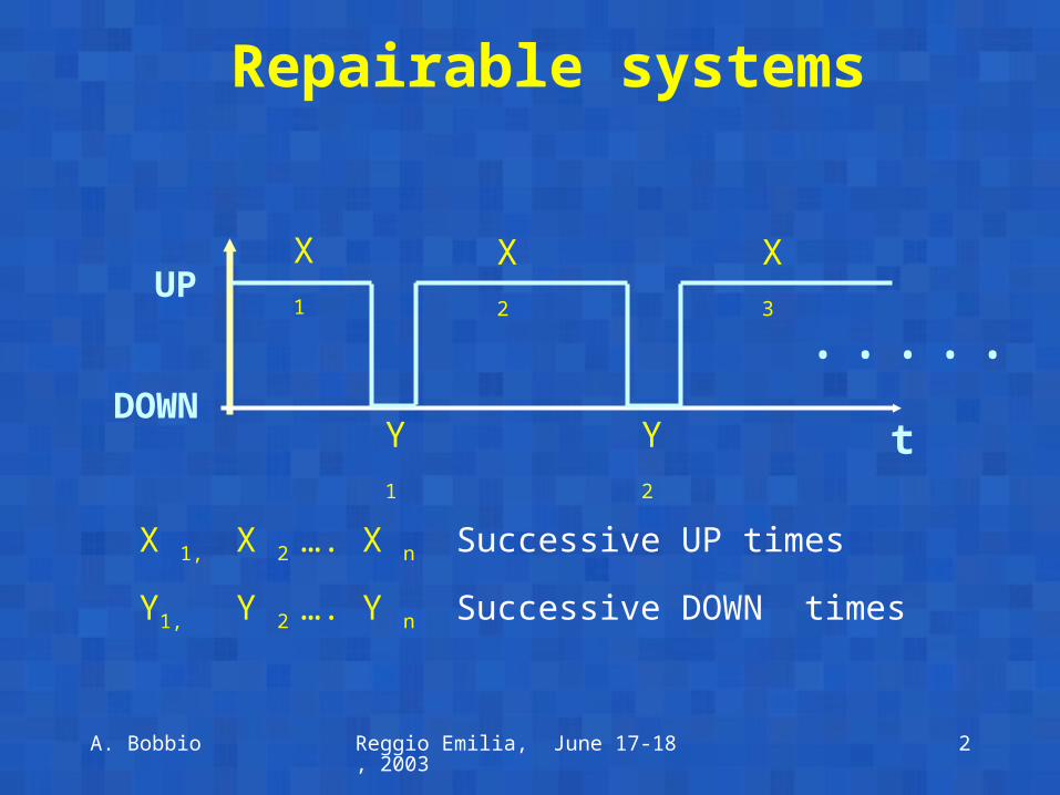
Repairable systems
X 1, X 2 …. X n Successive UP times
Y1, Y 2 …. Y n Successive DOWN times
t
UP
DOWN
X 1 X 2 X 3
Y 1 Y 2
• • • • •

A. Bobbio Reggio Emilia, June 17-18, 2003 3
Repairable systems
The usual hypothesis in modeling repairable systems is that:
The successive UP times X 1, X 2 …. X n are i.i.d. random variable: i.e. samples from a common cdf F (t)
The successive DOWN times Y1, Y 2 …. Y n are i.i.d. random variable: i.e. samples from a common cdf G (t)
A. Bobbio Reggio Emilia, June 17-18, 2003 4
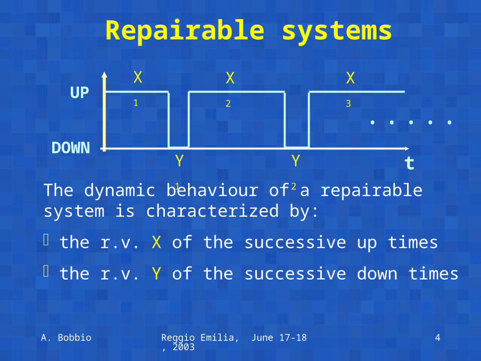
Repairable systems
The dynamic behaviour of a repairable system is characterized by:
the r.v. X of the successive up times
the r.v. Y of the successive down times
t
UP
DOWN
X 1 X 2 X 3
Y 1 Y 2
• • • • •

A. Bobbio Reggio Emilia, June 17-18, 2003 5
MaintainabilityLet Y be the r.v. of the successive down times:
G(t) = Pr { Y t } (maintainability)
d G(t) g (t) = ——— (density) dt g(t) h g (t) = ———— (repair rate) 1 - G(t)
MTTR = t g(t) dt (Mean Time To Repair) 0
A. Bobbio Reggio Emilia, June 17-18, 2003 6
Availability
The availability A(t) of an item at time t is the probability that the item is correctly working at time t.
The measure to characterize a repairable system is the availability (unavailability):
A. Bobbio Reggio Emilia, June 17-18, 2003 7
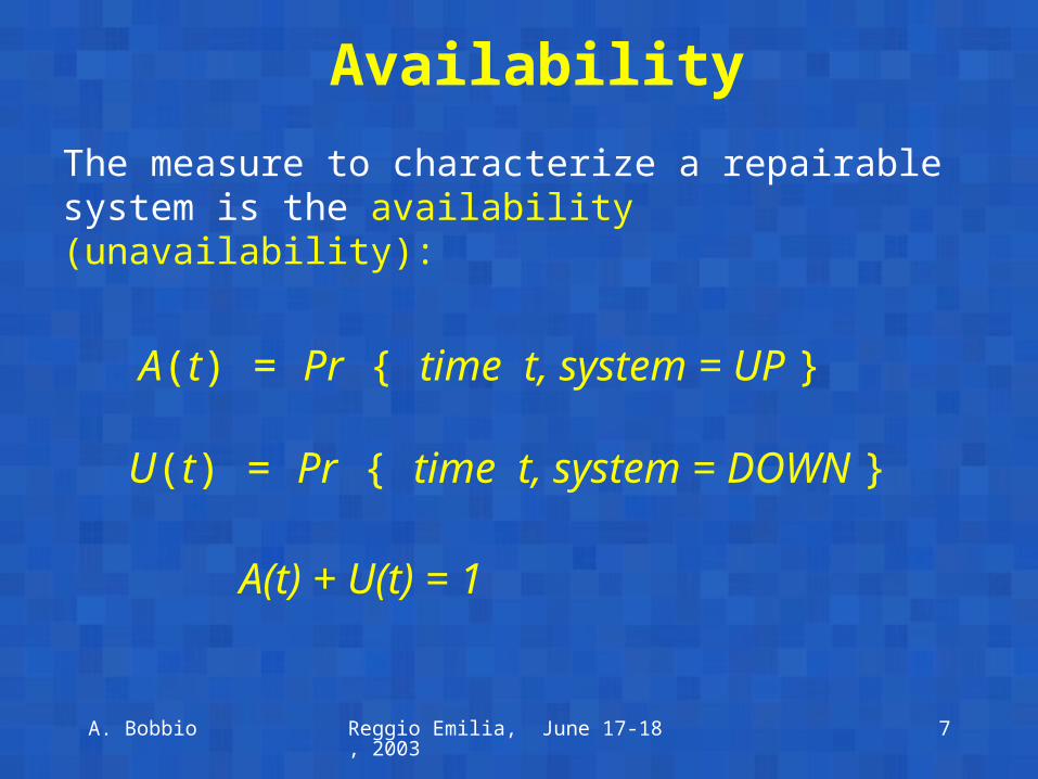
Availability
The measure to characterize a repairable system is the availability (unavailability):
A(t) = Pr { time t, system = UP }
U(t) = Pr { time t, system = DOWN }
A(t) + U(t) = 1
A. Bobbio Reggio Emilia, June 17-18, 2003 8
Definition of Availability
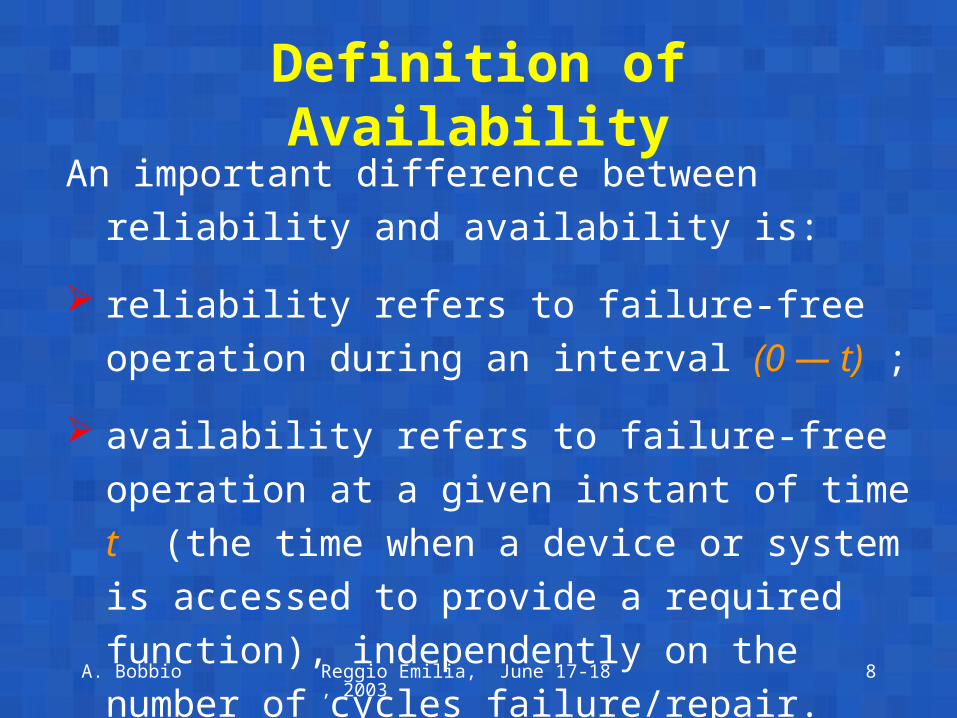
An important difference between reliability and availability is:
reliability refers to failure-free operation during an interval (0 — t) ;
availability refers to failure-free operation at a given instant of time t (the time when a device or system is accessed to provide a required function), independently on the number of cycles failure/repair.
A. Bobbio Reggio Emilia, June 17-18, 2003 9
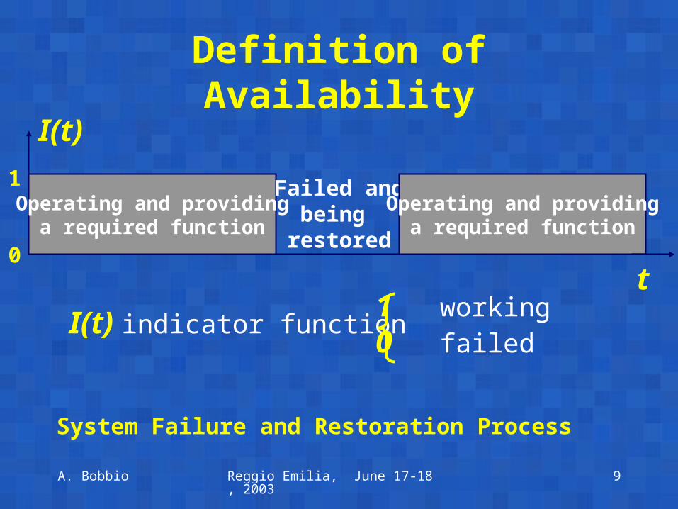
Definition of Availability
Operating and providinga required function
Failed andbeing
restored
1Operating and providing
a required function
System Failure and Restoration Process
tI(t) indicator function
0
I(t)
1 working0 failed
A. Bobbio Reggio Emilia, June 17-18, 2003 10
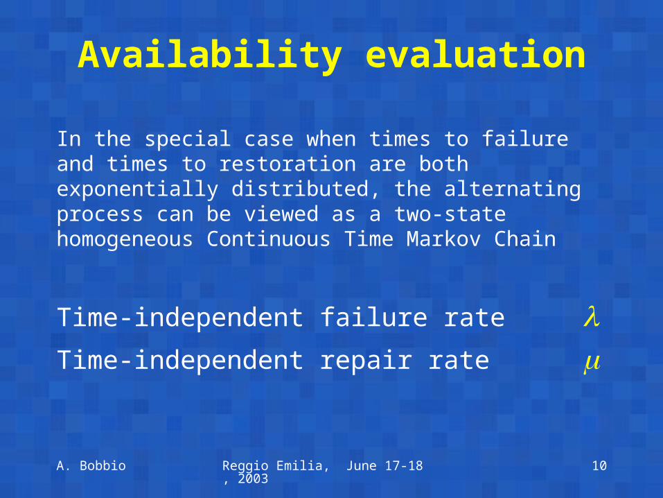
Availability evaluation
In the special case when times to failure and times to restoration are both exponentially distributed, the alternating process can be viewed as a two-state homogeneous Continuous Time Markov Chain
Time-independent failure rate Time-independent repair rate
A. Bobbio Reggio Emilia, June 17-18, 2003 11
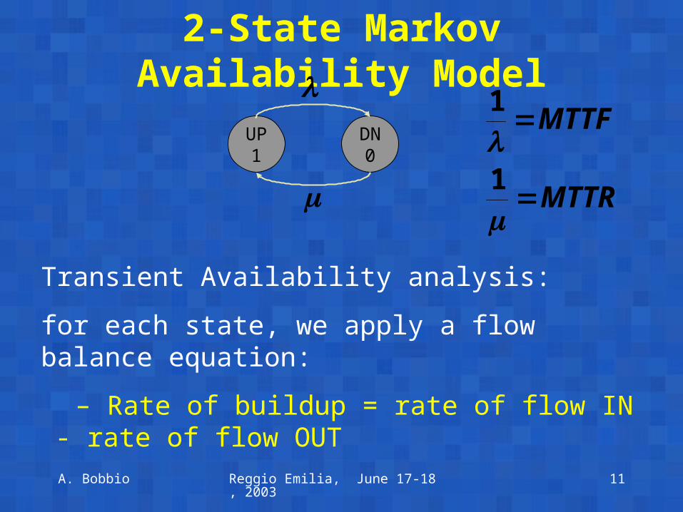
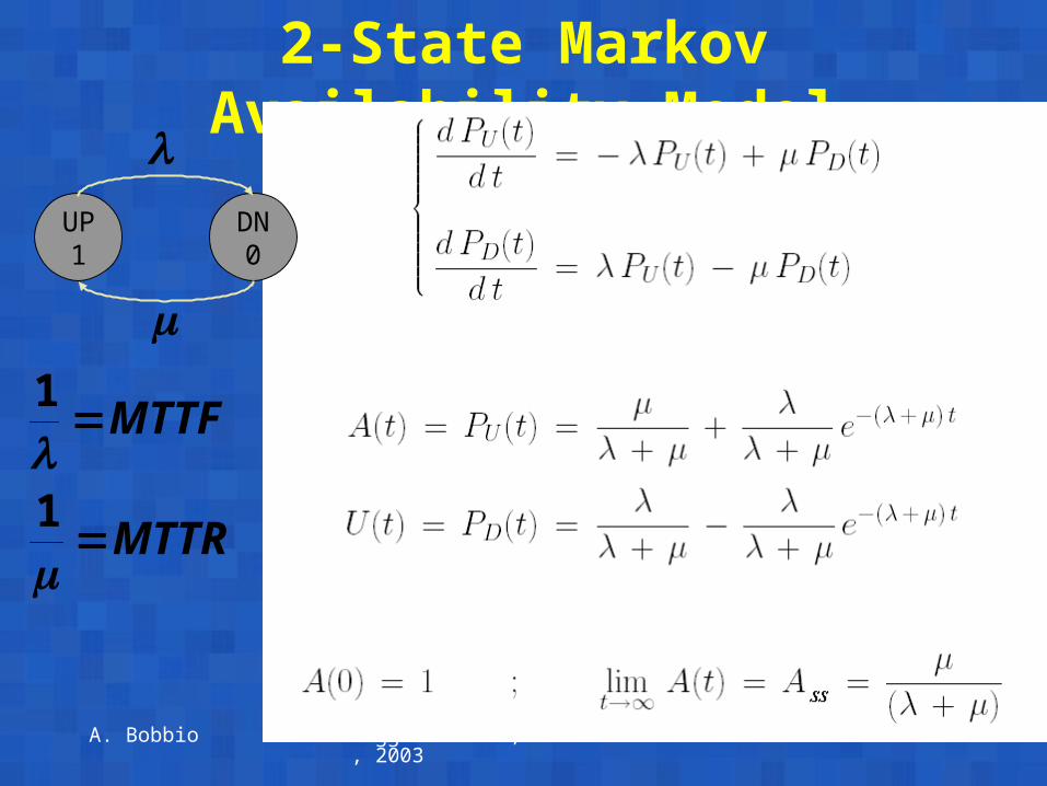
2-State Markov Availability Model
MTTR
MTTF
1
1UP1
DN0
Transient Availability analysis:
for each state, we apply a flow balance equation:
– Rate of buildup = rate of flow IN - rate of flow OUT
A. Bobbio Reggio Emilia, June 17-18, 2003 12
2-State Markov Availability Model
MTTR
MTTF
1
1
UP1
DN0
A. Bobbio Reggio Emilia, June 17-18, 2003 13
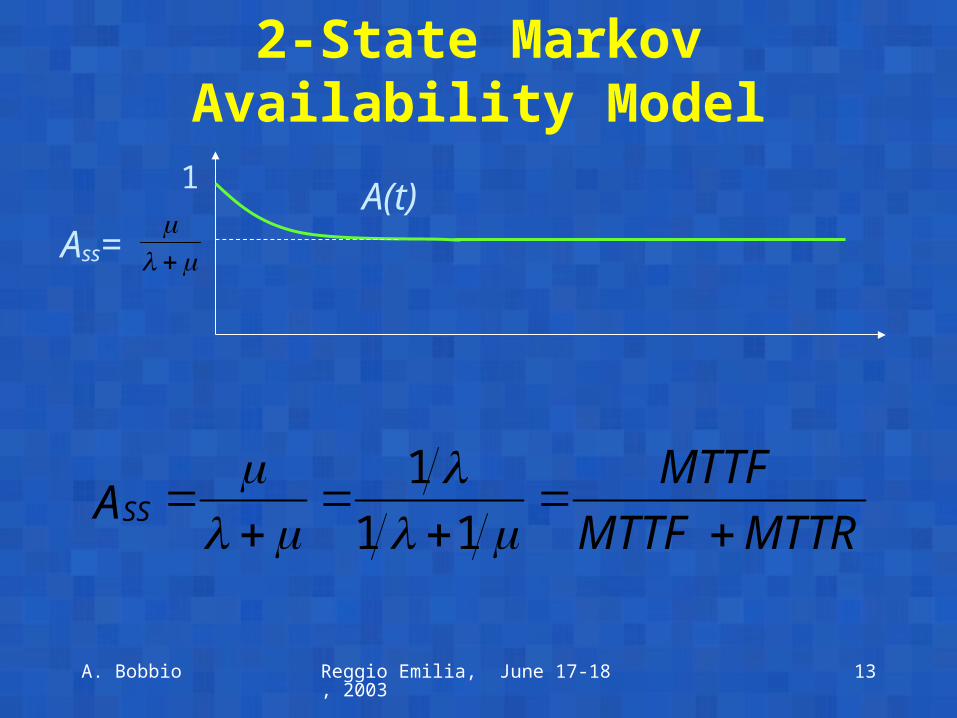
2-State Markov Availability Model
1 A(t)Ass=
MTTRMTTFMTTF
ASS
111
A. Bobbio Reggio Emilia, June 17-18, 2003 14
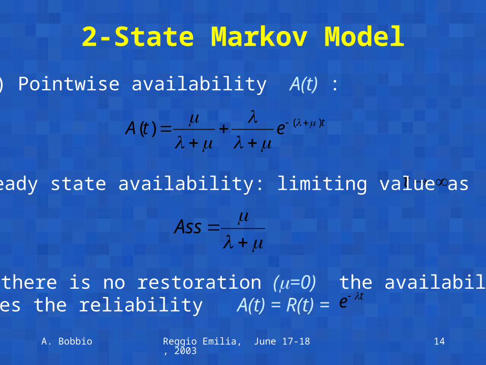
2-State Markov Model
tetA )()(
Ass
t
te
1) Pointwise availability A(t) :
2) Steady state availability: limiting value as
3) If there is no restoration (=0) the availability becomes the reliability A(t) = R(t) =
A. Bobbio Reggio Emilia, June 17-18, 2003 15
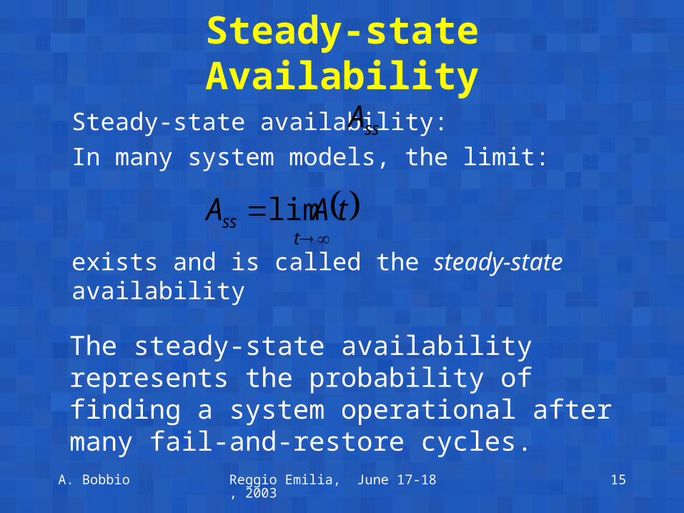
Steady-state Availability
Steady-state availability:In many system models, the limit:
exists and is called the steady-state availability
t
ss tAA lim
ssA
The steady-state availability represents the probability of finding a system operational after many fail-and-restore cycles.
A. Bobbio Reggio Emilia, June 17-18, 2003 16
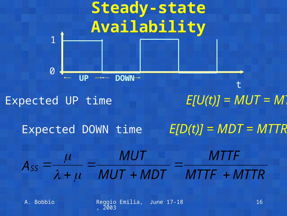
Steady-state Availability1
t0
UP DOWN
Expected UP time E[U(t)] = MUT = MTTF
Expected DOWN time E[D(t)] = MDT = MTTR
MTTRMTTFMTTF
MDTMUTMUT
ASS
A. Bobbio Reggio Emilia, June 17-18, 2003 17
Availability: Example (I)Let a system have a steady state availability
Ass = 0.95
This means that, given a mission time T, it is expected that the system works correctly for a total time of: 0.95*T.
Or, alternatively, it is expected that the system is out of service for a total time:
Uss * T = (1- Ass) * T
A. Bobbio Reggio Emilia, June 17-18, 2003 18
Availability: Example (II)Let a system have a rated productivity of W $/year.
The loss due to system out of service can be estimated as:
Uss * W = (1- Ass) * W
The availability (unavailability) is an index to estimate the real productivity, given the rated productivity.
Alternatively, if the goal is to have a net productivity of W $/year, the plant must be designed such that its rated productivity W’ should satisfy:
Uss * W’ = W
A. Bobbio Reggio Emilia, June 17-18, 2003 19
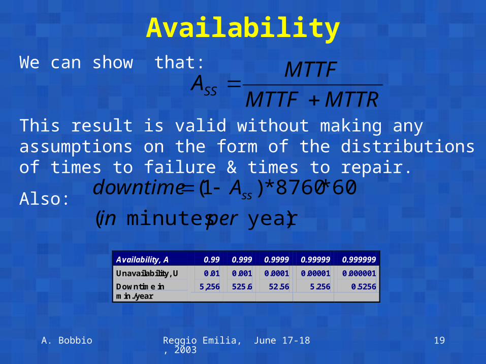
AvailabilityWe can show that:
This result is valid without making any assumptions on the form of the distributions of times to failure & times to repair.
Also:
MTTRMTTFMTTFASS
)yearminutes(60*8760*)1(
perinAdowntime ss
Availability, A 0.99 0.999 0.9999 0.99999 0.999999 Unavailability, U Downtime in min./year
0.01 5,256
0.001 525.6
0.0001 52.56
0.00001 5.256
0.000001 0.5256
A. Bobbio Reggio Emilia, June 17-18, 2003 20
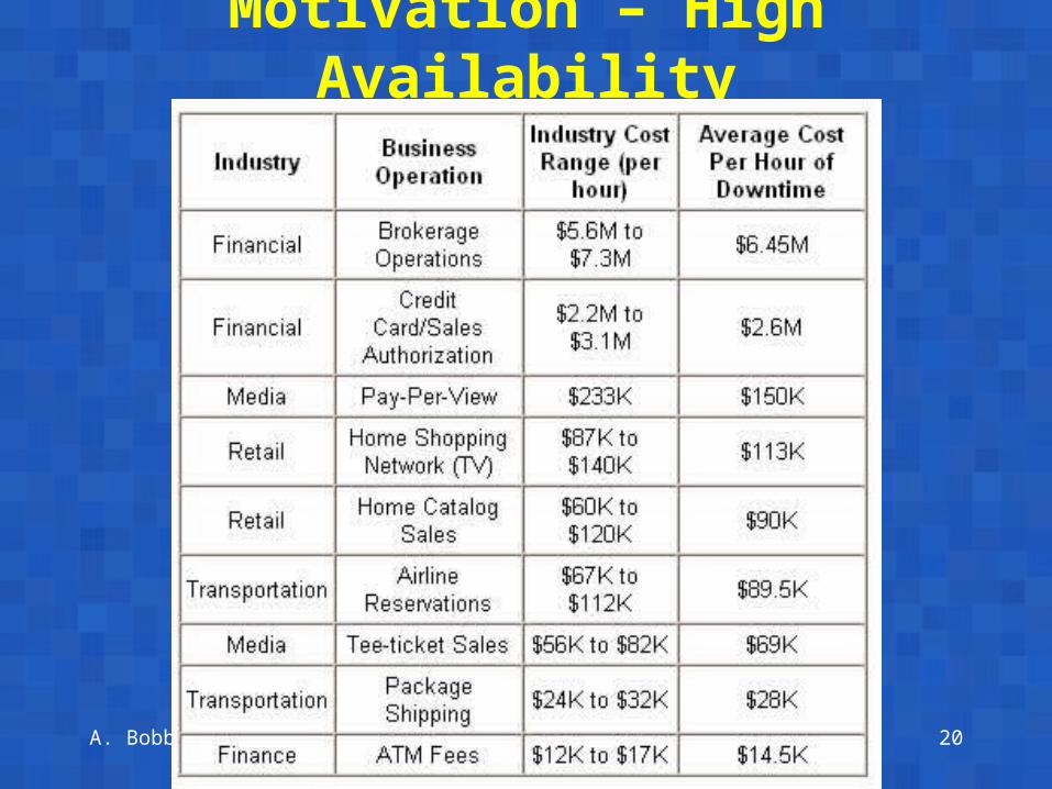
Motivation – High Availability
A. Bobbio Reggio Emilia, June 17-18, 2003 21
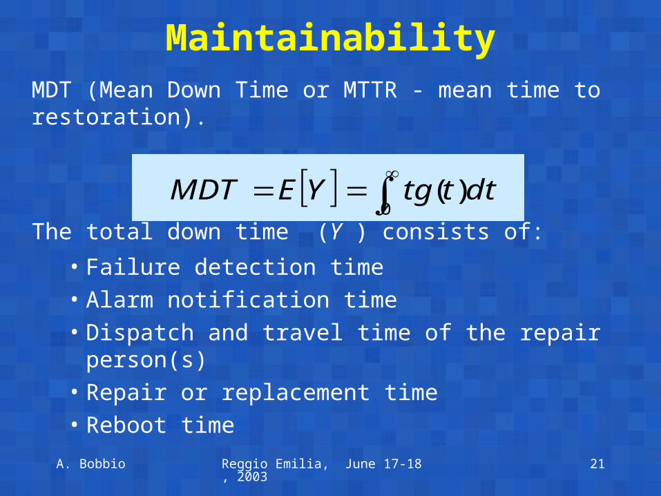
MDT (Mean Down Time or MTTR - mean time to restoration).
The total down time (Y ) consists of:• Failure detection time• Alarm notification time• Dispatch and travel time of the repair person(s)• Repair or replacement time• Reboot time
0
)( dtttgYEMDT
Maintainability
A. Bobbio Reggio Emilia, June 17-18, 2003 22
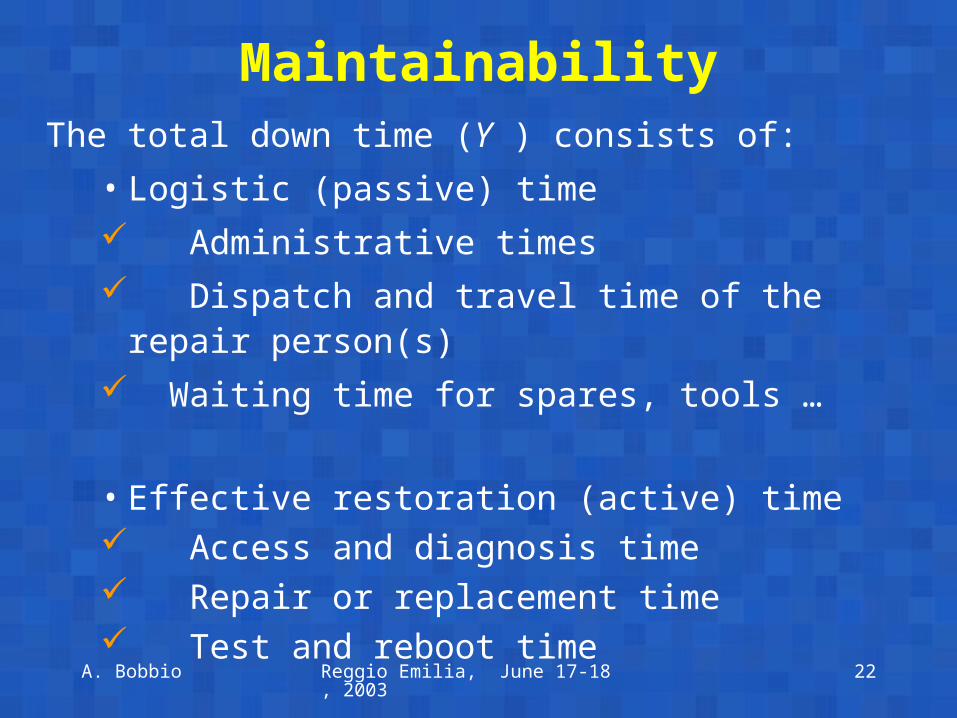
The total down time (Y ) consists of:• Logistic (passive) time Administrative times Dispatch and travel time of the repair person(s) Waiting time for spares, tools …
• Effective restoration (active) time Access and diagnosis time Repair or replacement time Test and reboot time
Maintainability
A. Bobbio Reggio Emilia, June 17-18, 2003 23
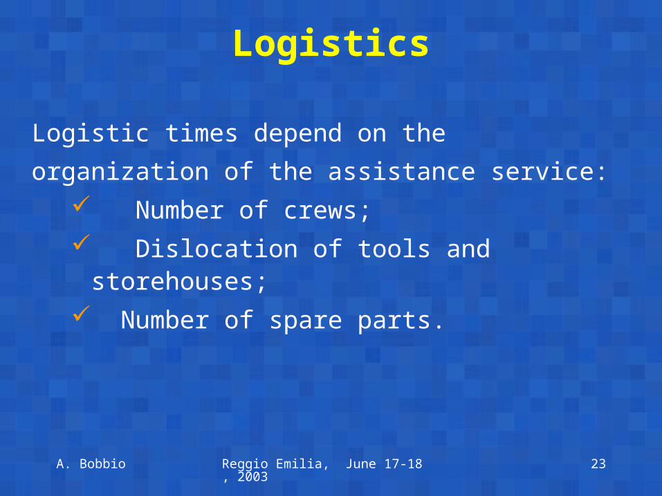
Logistic times depend on the organization of the assistance service:
Number of crews; Dislocation of tools and storehouses; Number of spare parts.
Logistics
A. Bobbio Reggio Emilia, June 17-18, 2003 24
The number of spares
A. Bobbio Reggio Emilia, June 17-18, 2003 25
The total cost of a maintenance action consists of: Cost of spares and replaced parts Cost of person/hours for repair Down-time cost (loss of productivity)
Maintenance Costs
The down-time cost (due to a loss of productivity) can be the most relevant cost factor.
A. Bobbio Reggio Emilia, June 17-18, 2003 26
Is the sequence of actions that minimizes the total cost related to a down time:
Reactive maintenance: maintenance action is triggered by a failure.
Proactive maintenance: preventive maintenance policy.
Maintenance Policy

A. Bobbio Reggio Emilia, June 17-18, 2003 27
Life Cycle Cost