arX

iv:2

108.

0478

2v1

[st

at.M

L]

10

Aug

202

1

Bandit Algorithms for Precision Medicine

Yangyi Lu∗, Ziping Xu∗, Ambuj Tewari

yylu,zipingxu,tewaria@umich.edu

Department of Statistics

University of Michigan

August 11, 2021

1 Introduction

The Oxford English Dictionary defines precision medicine as “medical care designed to optimize efficiencyor therapeutic benefit for particular groups of patients, especially by using genetic or molecular profiling.”It is not an entirely new idea: physicians from ancient times have recognized that medical treatment needsto consider individual variations in patient characteristics (Konstantinidou et al., 2017). However, the mod-ern precision medicine movement has been enabled by a confluence of events: scientific advances in fieldssuch as genetics and pharmacology, technological advances in mobile devices and wearable sensors, andmethodological advances in computing and data sciences.

This chapter is about bandit algorithms: an area of data science of special relevance to precision medicine.With their roots in the seminal work of Bellman, Robbins, Lai and others, bandit algorithms have cometo occupy a central place in modern data science (see the book by Lattimore and Szepesvári (2020) for anup-to-date treatment). Bandit algorithms can be used in any situation where treatment decisions need to bemade to optimize some health outcome. Since precision medicine focuses on the use of patient characteristicsto guide treatment, contextual bandit algorithms are especially useful since they are designed to take suchinformation into account.

The role of bandit algorithms in areas of precision medicine such as mobile health and digital phenotypinghas been reviewed before (Tewari and Murphy, 2017; Rabbi et al., 2019). Since these reviews were published,bandit algorithms have continued to find uses in mobile health and several new topics have emerged in theresearch on bandit algorithms. This chapter is written for quantitative researchers in fields such as statistics,machine learning, and operations research who might be interested in knowing more about the algorithmicand mathematical details of bandit algorithms that have been used in mobile health.

We have organized this chapter to meet two goals. First, we want to provide a concise exposition ofbasic topics in bandit algorithms. Section 2 will help the reader become familiar with basic problem setupsand algorithms that appear frequently in applied work in precision medicine and mobile health (see, forexample, Paredes et al. (2014); Piette et al. (2015); Rabbi et al. (2015); Piette et al. (2016); Yom-Tov et al.(2017); Rindtorff et al. (2019); Forman et al. (2019); Liao et al. (2020); Ameko et al. (2020); Aguilera et al.(2020); Tomkins et al. (2021)). Second, we want to highlight a few advanced topics that are important formobile health and precision medicine applications but whose full potential remains to be realized. Section 3will provide the reader with helpful entry points into the bandit literature on non-stationarity, robustness tocorrupted rewards, satisfying additional constraints, algorithmic fairness, and causality.

∗These authors made equal contributions to the writing of this chapter.

1

2 Basic Topics

In this section, we begin by introducing the most simple of all bandit problems: the multi-armed bandit.Then we discuss a more advanced variant called contextual bandit that is especially suitable for precisionmedicine applications. The last topic we discuss in this section is offline learning which deals with algorithmsthat can use already collected data. The offline learning setting is to be contrasted with the online learningsetting where the bandit algorithm has control over the data it collects.

2.1 Multi-armed Bandit

In recent years, the multi-armed bandit (MAB) framework has attracted a lot of attention in many applicationareas such as healthcare, marketing, and recommendation systems. MAB is a simple model that describesthe interaction between an agent1 and an environment. At every time step, the agent makes a choice from anaction2 set and receives a reward. The agent may have different goals, such as maximizing the (discounted)cumulative reward within a time horizon, identifying the best arm, or competing with the arm with the bestrisk-return trade-off etc. In this section, we focus on maximizing the cumulative rewards for simplicity. Animportant observation is that the agent needs to balance between exploration and exploitation to achieveits goal of receiving high cumulative reward. That is, both under-explored arms as well as tested-and-triedarms with high rewards should be selected often but for different reasons: the former have the potential toachieve high rewards and the latter are already confirmed to be good based on the past experience.

To formally define the bandit framework, we start with introducing some notation. Suppose the agentinteracts with the environment for T time steps, where T is called the horizon. In each round t ∈ [T ],the learner chooses an action At from the action set A and receives a corresponding reward Rt ∈ R. Wedenote the cardinality of A by K. The choice of At depends on the action/reward history up to time t− 1:Ht−1 = (A1, R1, . . . , At−1, Rt−1). A policy πt is defined as a mapping from the history up to time t − 1 tothe actions. For short, we use π as the sequence of policies (π0, . . . , πT−1).

In a healthcare setting, the fundamental pattern that often occurs is the following. Of course, this simplepattern fails to capture the full complexity of decision making in healthcare, but it is a reasonable startingpoint, especially for theoretical analysis.

Algorithm 1 Bandit Framework in Healthcare

Input: Available treatment options, treatment period length T .for t = 1, . . . , T do

A treatment option (action) is selected and delivered to the patient.Patient’s health outcome (reward) following the treatment is recorded.

end for

In the remainder of this section, we will review bandit algorithms that learn good decision policies overtime. We focus on the two key settings: stochastic bandit and adversarial bandit. In both settings, thealgorithms aim at minimizing their regret, which measures the difference between the maximal reward onecan get, and the reward obtained by the algorithm. We will formally define regret in each setting.

2.1.1 Stochastic Multi-armed Bandit

A stochastic bandit is a set of distributions ν = (Pa : a ∈ A) and we define the environment class E as a setof such distributions

E = ν = (Pa : a ∈ A) : Pa ∈ Ma for all a ∈ A,1Also referred to as a learner, statistician, or decision maker.2Since the historical roots of probability theory lie in gambling and casinos, it is not surprising that the MAB terminology

comes from imagining a slot machine in a casino. A slot machine is also called a “one-armed bandit” as it robs you of yourmoney. Therefore, we will use actions and arms interchangeably.

2

where for each a, Ma is a set of distributions. For unstructured bandits, playing one action cannot helpthe agent deduce anything about other actions. Environment classes that are not unstructured are calledstructured, such as linear bandits (Abbasi-Yadkori et al., 2011), low-rank bandits (Lu et al., 2021b) andcombinatorial bandits (Cesa-Bianchi and Lugosi, 2012) etc. Throughout this chapter, we assume all banditinstances are EKSG(1), which means the reward distribution for all K arms is 1-subgaussian.

Definition 1 (Subgaussianity). A random variable X is σ-subgaussian if for all λ ∈ R, E[eλX

]≤ eλ2σ2/2.

It is not hard to see from the definition that many well-known distributions are subgaussian, e.g., anybounded-domain distribution, Bernoulli distribution and Gaussian distributions. Intuitively, a subgaussiandistribution has tails no heavier than a Gaussian distribution. Many nice concentration inequalities havebeen developed for subgaussian variables and are widely used in the proofs of bandit algorithms.

In the process of interactions, once the agent performs action at following a particular policy, the en-vironment samples a reward Rt from the distribution Pat

. The combination of an environment and agentpolicy induces a probability measure on the sequence of outcomes a1, R1, . . . , aT , RT . A standard stochasticMAB protocol is following. At every time step t = 1, . . . , T , the learning agent

1. picks an action at ∈ A following policy πt−1,

2. receives reward Rt ∼ Pat,

3. updates its policy to πt.

We note that Patis the conditional reward distribution of Rt given Ht−1, at and πt is a function from

Ht−1 to A. The expected reward of action a is defined by µa(ν)def= Eν [R|a] =

∫∞

−∞ rdPa(r), where R is usedas the reward variable. Then the maximum expected reward and the optimal action are given by

µ∗(ν) = maxa∈A

µa(ν) and a∗(ν) ∈ argmaxa∈A µa(ν).

According to above definition, more than one optimal actions can exist and the optimal policy is to selectan optimal action at every round. For actions whose expected rewards are less than optimal actions, we callthem sub-optimal actions and define the reward gap between action a and a∗(ν) by ∆a := µ∗(ν)− µa(ν).

As mentioned earlier, the learner’s goal is to maximize the cumulative reward ST =∑T

t=1Rt. We nowdefine a performance metric called regret which is the difference between the expected reward that π∗(ν)can obtain and E[ST ]. Minimizing the regret is equivalent to maximizing the reward. The reason why we donot directly optimize ST is that the cumulative rewards depends on the environment and it is hard to tellwhether a policy is good or not by merely looking at the cumulative rewards unless it is compared to a goodpolicy. So we define the problem-dependent regret of a policy π on bandit instance ν by

RegT (π, ν) = Tµ∗(ν)− E[ST ],

where the expectation is taken over actions and rewards up to time T . The worst-case regret of a policy πis defined by

RegT (π) = supν∈E

RegT (π, ν).

We will drop π and ν from the regret when they are clear from the context.

Remark about Pure Exploration. Throughout this chapter, we focus on minimizing regret by bal-ancing exploration and exploitation. We also want to point out that in a different setting, the explorationcost may not be a concern and the agent just wants to output a final recommendation for the best armafter an exploration phase. Problems of this type are called pure exploration problems. In such cases, algo-rithms are usually evaluated by sample complexity or simple regret (Bubeck et al., 2009). Pure explorationis also related to randomized controlled trials (RCTs) including modern variants that involve sequential

3

Algorithm 2 Explore-then-Commit (ETC)

1: Input: action space A, where K = |A|, number of exploration steps, m, horizon T .2: for t = 1, . . . , T do3: if t ≤ mK then4: play At = (t mod K) + 1.5: else6: play At = argmaxa µa(mK).7: end if8: receive Rt.9: end for

randomization such as sequential multiple assignment randomized trials (SMARTs) (Lei et al., 2012) andmicro-randomized trials (MRTs) (Klasnja et al., 2015). Randomized trials are typically designed to enableestimation of treatment effects with sufficient statistical power. Since the concerns of pure exploration andrandomized controlled trials are different from those of bandit algorithms, we do not discuss them furtherin this chapter. However, note that in an actual application, methodology from bandits and randomizedtrials may need to be integrated. Researchers may start off with a randomized trial and follow it up withbandit algorithm in the next iteration of their health app. They can also decide to run a randomized trial forone health outcome while simultaneously running a bandit for a different outcome (e.g., an outcome relatedto user engagement with the health app) in the same study. There is also ongoing work (Yao et al., 2020;Zhang et al., 2021) on enabling the kind of statistical analysis done after randomized trials on data collectedvia online bandit algorithms.

Explore-then-Commit (ETC). We start with a simple two-stage algorithm: Explore-then-Commit(ETC). In the first stage of ETC, the learner plays every arm for a fixed number of times (m) and ob-tain estimates of the expected rewards. In the second stage, the learner commits to the best arm accordingto the estimates in the first stage. For every arm a, let µa(t) denote the estimated expected reward up totime t:

µa(t) =1

Ta(t)

t∑

s=1

1As=aRs,

where Ta(t) =∑t

s=1 1As=a is the number of times action a has been performed up to round t.With the above definitions, we are ready to present the ETC in Algorithm 2. The overall performance of

ETC crucially depends on the parameterm. If m is too small, the algorithm cannot estimate the performanceof every arm accurately, so it is likely to exploit a sub-optimal arm in the second stage, which leads to highregret. If m is too big, the first stage (explore step) plays with sub-optimal arms for too many times,so that the regret can be large again. The art is to choose an optimal value for m in order to minimizethe total regret incurred in both stages. Specifically, ETC achieves O(T 2/3) worst-case regret3 by choosingm = O(T 2/3) (Lattimore and Szepesvári, 2020). Sub-linear regret O(T 2/3) performance is good as a startingpoint. Next, we will introduce another two classic algorithms which incur even less regret.

Upper Confidence Bound (UCB). There are several types of exploration strategies to select actionssuch as greedy, Boltzmann, optimism and pessimism. Suppose the agent has reward estimates µa for allactions. A greedy exploration strategy simply selects the action with the highest µa. A Boltzmann explo-ration strategy picks each action with probability proportional to exp(ηµa), where η is a tuning parameter.Boltzmann becomes greedy as η goes to infinity. For an optimism strategy, one picks the action with thehighest reward estimate plus some bonus term, i.e. argmaxa µa + bonusa. In contrast, a pessimism strategywould pick the action: argmaxa µa − bonusa.

3Ignoring parameters other than T .

4

Algorithm 3 Upper Confidence Bound (UCB)

1: Input: δ, A where K = |A|.2: for t = 1, . . . , T do3: play At = argmaxa∈A UCBa(t− 1, δ).4: receive reward Rt and update the upper confidence bound terms according to (1).5: end for

Out of these strategies, UCB algorithm follows the optimism strategy, in particular, a famous principlecalled optimism in the face of uncertainty (OFU), which means that one should act as if the environmentis the best possible one among those that are plausible given current experience. The reason OFU works isthat misplaced optimism gets corrected when under-explored actions are tried and low rewards are observed.In contrast, pessimism does not work (at least in the online setting; for the offline setting things can bedifferent (Jin et al., 2021)) since wrong beliefs about low performance of under-explored actions do not geta chance to get revised by collecting more data from those actions.

At every step t, the UCB algorithm updates a value called upper confidence bound defined for each actiona ∈ A and confidence level δ ∈ [0, 1] as follows.

UCBa(t− 1, δ) =

∞, if Ta(t− 1) = 0

µa(t− 1) +√

2 log(1/δ)Ta(t−1)∨1 , otherwise.

(1)

The learner chooses the action with the highest UCB value at each step. Overall, UCB (Algorithm 3)guarantees a O(

√T ) worst-case regret (where the informal O(·) notation hides constants and logarithmic

factors).According to the construction of upper confidence bounds, an action will be selected under two circum-

stances: under-explored (Ta(t − 1) small) or well-explored with good performance (µa(t − 1) large). Theupper confidence bound for an action gets close to its true mean after being selected for enough times. Asub-optimal action will only be played if its upper confidence bound is larger than that of the optimal arm.However, this is unlikely to happen too often. The upper confidence bound for the sub-optimal action willeventually fall below that of the optimal action as we play the sub-optimal actions more times. We presentthe regret guarantee for UCB (Algorithm 3) in Theorem 1.

Theorem 1 (Regret for UCB Algorithm). If δ = 1/T , then the problem-dependent regret of UCB, as definedin Algorithm 3, on any 1-subgaussian bandit ν is bounded by

RegT (UCB, ν) ≤ 3∑

a∈A

∆a +∑

a:∆a>0

16 logT

∆a, (2)

where ∆a := µ∗(ν)− µa(ν) represents the corresponding gap term. The worst-case regret bound of UCB is:

RegT (UCB) = O(√KT logT ). (3)

Proof. We only present the worst-case regret for simplicity. For the problem-dependent regret proof, werefer the reader to Chapter 7 in Lattimore and Szepesvári (2020).

We define a good event E as follows:

E :=

|µa(t− 1)− µa| ≤

√2 log(1/δ)

Ta(t− 1) ∨ 1, ∀t ∈ [T ], a ∈ A

.

By Hoeffding inequality and union bound, one can show that P(Ec) ≤ 2TKδ4. Next, we decompose the

5

regret.

RegT (UCB) = E

[T∑

t=1

µ∗ −UCBa∗(t− 1, δ) + UCBa∗(t− 1, δ)−UCBAt(t− 1, δ) + UCBAt

(t− 1, δ)− µAt

]

≤ E

[T∑

t=1

µ∗ −UCBa∗(t− 1, δ) + UCBAt(t− 1, δ)− µAt

].

The inequality in above expression is due to the action selection criterion in UCB algorithm. Condition onevent E, we have µ∗ − UCBa∗(t − 1, δ) ≤ 0 for all t ∈ [T ]; otherwise, the regret can be bounded by 2T .Combining these arguments, we have

RegT (UCB) ≤ P(Ec) · 2T + P(E) · E[

T∑

t=1

UCBAt(t− 1, δ)− µAt

| E]

≤ 4T 2Kδ4 + 2E

[T∑

t=1

√2 log (1/δ)

TAt(t− 1) ∨ 1

](By definition of event E)

≤ 4T 2Kδ4 +√8 log (1/δ)

∑

a∈A

T∑

t=1

E

[√1

TAt(t− 1) ∨ 1

1At=a

]

≤ 4T 2Kδ4 +√8 log (1/δ)

∑

a∈A

∫ Ta(T )

1

√1/sds

≤ 4T 2Kδ4 +√8 log (1/δ)

√KT = O(

√KT logT ) (Set δ = 1/T ).

The last inequality in above is by Cauchy-Schwarz inequality.

The UCB family has many variants, one of which is to replace the upper confidence bound for every

action by µa(t− 1) +√2 log

(1 + t log2(t)

)/Ta(t− 1). Even though the regret dominant terms (

√KT logT

and∑

a:∆a>0log T∆a

) for this version has the same order as those of Algorithm 3, the leading constants for thetwo dominant terms become smaller.

Then one may ask the question: is it possible to further improve the regret bound of UCB and abovevariant? The answer is yes. Audibert et al. (2009) proposed an algorithm called MOSS (Minimax OptimalStrategy in the Stochastic case). MOSS replaces the upper confidence bounds in Algorithm 3 by

µa(t− 1) +

√√√√maxlog(

TKTa(t−1)

), 0

Ta(t− 1).

Under this construction, the worst-case regret of MOSS is guaranteed to be only O(√KT ).

However, MOSS is not always good. One can easily construct regimes where the problem-dependentregret of MOSS is worse than UCB (Lattimore, 2015). On the other hand, the improved UCB algorithmproposed by Auer and Ortner (2010) satisfies a problem-dependent regret that is similar to (1), but the worst-case regret is O(

√KT logK). Later on, by carefully constructing the upper confidence bounds, Optimally

Confidence UCB algorithm (Lattimore, 2015) and AdaUCB algorithm (Lattimore, 2018) are shown to achieveO(√KT ) worst-case regret and their problem-dependent regret bounds are also not worse than that of the

UCB algorithm. There are many more UCB variants in the literature that we do not cover in this chapter.The reader may refer to Table 2 in Lattimore (2018) for a comprehensive summary.

Successive Elimination (SE). We now describe the SE algorithm that also relies on the upper confidencebound calculations. The idea is similar to UCB such that a sub-optimal arm is very unlikely to have large a

6

Algorithm 4 Successive Elimination (SE)

1: Input: δ,A where K = |A|.2: while A contains more than one arm do3: play every arm in A once and update the UCBs and LCBs using (1) and (4).4: Eliminate all arms a s.t. ∃a′ ∈ A with UCBa(t− 1, δ) < LCBa′(t− 1, δ).5: end while

upper confidence bound if it has been selected for enough times. At every round, SE maintains a confidenceinterval for the mean reward of every arm and removes all arms whose reward upper bound is smaller thanthe lower bound of the biggest estimated reward arm. The procedure ends when there is only one armremained. We describe the SE algorithm in Algorithm 4 and define the UCB terms as (1) and LCB terms as

LCBa(t− 1, δ) =

∞, if Ta(t− 1) = 0

µa(t− 1)−√

2 log(1/δ)Ta(t−1)∨1 , otherwise.

(4)

SE was first proposed in Even-Dar et al. (2006) along with a similar action elimination based algorithm:Median Elimination (ME). They studied the probably approximately correct (PAC) setting (Haussler and Warmuth,2018). In particular, Even-Dar et al. (2006) shows that for given K arms, it suffices to pull the arms forO(Kε2 log(1/δ) times to find an ε-optimal arm with probability at least 1− δ. It is not hard to prove that SEalso satisfies the following regret bound.

Theorem 2 (Regret for SE Algorithm). If δ = 1/T , the worst-case regret of SE over 1-subgaussian banditenvironments is bounded by

RegT (SE) = O(√KT logT ). (5)

Proof. Without loss of generality, we assume the optimal arm a∗ is unique. Define the event E by |µa(t)−µa| ≤ ca(t, δ), ∀a, t, where ca(t, δ) =

√2 log(1/δ)Ta(t)∨1 denotes the confidence set width. By Hoeffding inequality

and union bound, one can show that P(Ec) ≤ 2δ4TK.Define t as the last round when arm a is not eliminated yet. According to the elimination criterion in

SE, the reward gap term can be bounded as:

∆a := µ∗ − µa ≤ 2(ca∗(t, δ) + ca(t, δ)) = O(ca(t, δ)).

The last equality holds as Ta(t) and Ta∗(t) differ at most by 1 by construction. Since t is the last round abeing played, we have Ta(t) = Ta(T ) and ca(t) = ca(T ), which implies below property for all non-optimalarms a:

∆a ≤ O(√

log(1/δ)

Ta(T )

).

We thus obtain that under event E,

T∑

t=1

E[µ∗ − µat|E] ≤

∑

a∈A\a∗

Ta(T )∆a ≤ O(√

log(1/δ))∑

a∈A

√Ta(T ) ≤ O(

√KT log(1/δ)),

where the last inequality is by Cauchy-Schwarz inequality. Take δ = 1/T , RegT (SE) = O(√KT logT ) by

conditional expectation calculations.

7

Algorithm 5 Thompson Sampling (TS)

1: Input: Bayesian bandit environment (E ,B(E), Q, P ) (B(·) is the Borel set), action set A with |A| = K.

2: for t = 1, . . . , T do3: Sample νt ∼ Q(·|A1, R1, . . . , At−1, Rt−1).4: Play At = argmaxi∈[K] µi(νt).5: end for

Thompson Sampling (TS). All of the methods we have mentioned so far select their actions based ona frequentist view. TS uses one of the oldest heuristic (Thompson, 1933) for choosing actions and addressesthe exploration-exploitation dilemma based on a Bayesian philosophy of learning. The idea is simple. Beforethe game starts, the agent chooses a prior distribution over a set of possible bandit environments. At everyround, the agent samples an environment from the posterior and acts according to the optimal action inthat environment. The exploration in TS comes from the randomization over bandit environments. At thebeginning, the posterior is usually poorly concentrated, then the policy will likely explore. As more databeing collected, the posterior tends to concentrate towards the true environment and the rate of explorationdecreases. We present the TS algorithm in Algorithm 5.

To formally describe how TS works, we start with several definition related to Bayesian bandits.

Definition 2 (K-armed Bayesian bandit environment). A K-armed Bayesian bandit environment is a tuple(E ,G, Q, P ) where (E ,G) is a measurable space and Q is a probability measure on (E ,G) called the prior.P = (Pνa : ν ∈ E , a ∈ A) is the reward distribution for arms in bandit ν, where |A| = K.

Given a K-armed Bayesian bandit environment (E ,G, Q, P ) and a policy π, the Bayesian regret is definedas:

BRegT (π,Q) =

∫

E

RegT (π, ν)dQ(ν).

TS has been analyzed in both of the frequentist and the Bayesian settings and we will start with theBayesian results.

Theorem 3 (Bayesian Regret for TS Algorithm). For a K-armed Bayesian bandit environment (E ,G, Q, P )such that Pνa is 1-subgaussian for all ν ∈ E and a ∈ [K] with mean in [0, 1]. Then the policy π of TS satisfies

BRegT (π,Q) = O(√KT logT ). (6)

Proof. The proof is quite similar to that of UCB. We abbreviate µa = µa(ν) and let a∗ = argmaxa∈[K] µa bethe optimal arm. Note that a∗ is a random variable depending on ν. For every a ∈ [K], we define a clippedupper bound term

UCBa(t− 1) = µa(t− 1) +

√2 log(1/δ)

1 ∨ Ta(t− 1),

where µa(t− 1) and Ta(t− 1) are defined in the same way as those in UCB. We define event E such that forall t ∈ [T ] and a ∈ A,

|µa(t− 1)− µa| <√

2 log(1/δ)

1 ∨ Ta(t− 1).

By Hoeffding inequality and union bound, one can show that P(Ec) ≤ 2TKδ4. This result will be used inlater steps.

8

Let Ft = σ(A1, R1, . . . , At, Rt) be the σ-algebra generated by the interaction sequence up to time t. Thekey insight for the whole proof is to observe below property from the definition of TS:

P(a∗|Ft−1) = P(At|Ft−1) a.s. (7)

Using above property and BRegT = E

[∑Tt=1(µa∗ − µAt

)]= E

[∑Tt=1 E [(µa∗ − µAt

) | Ft−1]], we have

E [µa∗ − µAt| Ft−1] = E [µa∗ −UCBa∗(t− 1) + UCBAt

(t− 1)− µAt| Ft−1] ,

and thus

BRegT = E

[T∑

t=1

(µa∗ −UCBa∗(t− 1)) +T∑

t=1

(UCBAt(t− 1)− µAt

)

].

Conditioning on the high-probability event E, the first sum is negative and the second sum is of the orderO(√KT log(1/δ)), while BRegT ≤ 2T if conditioning on Ec. Take δ = 1/T , one can verify that BRegT =

O(√KT log T ).

Compared to the analysis for Bayesian regret, frequentist (worst-case) regret analysis for TS gets a lotmore technical. The key reason behind this is that the worst-case regret does not have an expectationwith respect to the prior and therefore the property in (7) cannot be used. Even though TS was well-known to be easy to implement and competitive with state of the art methods, it lacked worst-case regretanalysis for a long time. Significant progress was made by Agrawal and Goyal (2012) and Kaufmann et al.(2012). In Agrawal and Goyal (2012), the first logarithmic bound on the frequentist regret of TS was proven.Kaufmann et al. (2012) provided a bound that matches the asymptotic lower bound of Lai and Robbins(1985). However, both of these bounds were problem-dependent. The first near-optimal worst-case regretO(√KT log T ) was proved by Agrawal and Goyal (2013) for Bernoulli bandits with Beta prior, where the

reward is either zero or one. For TS that uses Gaussian prior, the same work proved a O(√KT logK) worst-

case regret. Jin et al. (2020) proposed a variant of TS called MOTS (Minimax Optimal TS) that achievesO(√KT ) regret.

2.1.2 Adversarial Multi-armed Bandit

In stochastic bandit models, the rewards are assumed to be strictly i.i.d. given actions. This assumption canbe violated easily in practice. For example, the health feedback for a patient after certain treatments mayvary slightly across times and the way it varies is usually unknown. In such scenarios, a best action thatmaximizes the total reward still exists, but algorithms designed for stochastic bandit environments are nolonger guaranteed to work. As a more robust counterpart to the stochastic model, we study the adversarialbandit model in this section, in which the assumption that a single action is good in hindsight is retainedbut the rewards are allowed to be chosen adversarially.

The adversarial bandit environment is often called as the adversary. In an adversarial bandit problem,the adversary secretly chooses reward vectors r := rtTt=1 where rt ∈ [0, 1]K corresponds to the rewardsover all actions at time t. In every round, the agent chooses a distribution over the actions Pt. An actionAt ∈ [K] is sampled from Pt and the agent receives the reward rtAt

. A policy π in this setting maps thehistory sequences to distributions over actions. We evaluate the performance of policy π by the expectedregret, which is the cumulative reward difference between the best fixed action and the agent’s selections:

RegT (π, r) = maxa∈A

T∑

t=1

rta − E

[T∑

t=1

rtAt

](8)

The worst-case regret of policy π is defined by

RegT (π) = supr∈[0,1]T×K

RegT (π, r). (9)

9

It may not be very clear at the beginning that why we define the regret by comparing to the fixed bestaction instead of the best action at every round. In the later case, the regret should be Reg′T (π, x) =

E

[∑Tt=1 maxa∈A rta −

∑Tt=1 rtAt

]. However, this definition provides the adversary too much power so that

for any policy, one can show Reg′T (π, r) can be Ω(T ) for certain reward vectors r ∈ [0, 1]K×T .

Remark on randomized policy: In stochastic bandit models, the optimal action is deterministic andthe optimal policy is simply to select the optimal action at every round. However, in adversarial banditsetting, the adversary has great power in designing the reward. It may know the agent’s policy and designthe rewards accordingly, so that a deterministic policy can incur linear regret. For example, we consider thereare two actions, whose reward is either 0 or 1 at any time. For a deterministic policy, the agent decides tochoose an action at time t. Then the adversary knows it and can set the reward of that action at time t to be0 and the reward of the unselected action to be 1. The cumulative regret will be T after T rounds. However,one can improve the performance by a randomized policy, e.g., choosing either action with probability 0.5,then the adversary cannot make you incur regret 1 at every round by manipulating the reward values forboth actions.

Exponential-weight algorithm for Exploration and Exploitation (EXP3). We now study one ofthe most famous adversarial bandit algorithm called EXP3. Before describing the algorithm, we define somerelated terms below. In a randomized policy, the conditional probability of the action a being played isdenoted by

Pta = P(At = a | A1, R1, . . . , At−1, Rt−1).

Assuming Pta > 0 almost surely for all policies, a natural way to define the importance-weighted estimatorof rta is

Rta =1At=aRt

Pta. (10)

Let Et[·] = E[· | A1, R1, . . . , At−1, Rt−1]. A simple calculation shows that Rta is conditionally unbiased, i.e.Et[Rta] = rta. However, the variance of estimator Rta can be extremely large when Pta is small and rta isnon-zero. Let Ata := 1At=a, then the variance of the estimator is:

Vt[Rta] = Et[R2ta]− r2ta = Et

[Atar

2ta

P 2ta

]− r2ta =

r2ta(1− Pta)

Pta.

An alternative estimator is:

Rta = 1− 1At=a

Pta(1−Rt). (11)

This estimator is still unbiased and its variance is

Vt[Rta] = y2ta1− Pta

Pta,

where we define yta = 1− rta.The best choice of the estimator Rta depends on the actual rewards. One should use (10) for small

rewards and (11) for large rewards. So far we have learned how to construct reward estimators for givensampling distributions Pta. EXP3 algorithm provides a way to design the Pta terms. Let St,a =

∑ts=1 Rsa

be the total estimated reward until the end of round t, where Rsi is defined in (11). We present EXP3 inAlgorithm 6.

Surprisingly, even though adversarial bandit problems look more difficult than stochastic bandit problemsdue to the strong power of the adversary, one can show that the adversarial regret for EXP3 algorithm hasthe same order as before, i.e. O(

√KT logT ).

10

Algorithm 6 Exponential-weight Algorithm for Exploration and Exploitation (Exp3)

1: Input: T,K, η2: Set S0,a = 0 for all a.3: for t = 1, . . . , T do

4: Calculate Pta ←exp(ηSt−1,a)

∑a′∈A exp(ηSt−1,a′ )

for all a ∈ [K]

5: Sample At from Pt and receive reward Rt

6: Calculate St,a ← St−1,a + 1− 1At=a(1−Rt)

Pta

7: end for

Theorem 4 (Regret for EXP3 Algorithm). Let r ∈ [0, 1]T×K. With learning rate η =√logK/(KT ), we

have

RegT (EXP3, r) ≤ 2√KT logK. (12)

Proof. The proof for EXP3 is different than those for the stochastic bandit algorithms. We first define theexpected regret relative to using action a in T rounds:

RegTa =T∑

t=1

rta − E

[T∑

t=1

Rt

].

According to the definition of the adversarial bandit regret, the final result will follow if we can bound RTa

for every a ∈ A. It’s not hard to show E[ST,a] =∑T

t=1 rta and Et[Rt] =∑

a∈A Ptarta =∑K

i=1 PtaE[Rta] hold

using the definition of Rta. Then we can re-write RTa as E

[ST,a − ST

], where ST =

∑Tt=1

∑a∈A PtaRta.

Let Wt =∑

a∈A exp(ηSt,a

), S0,a = 0 and W0 = K, then one can show that

exp(ηST,a

)≤∑

a′∈A

exp(ηST,a′

)=WT = K

T∏

t=1

Wt

Wt−1= K

T∏

t=1

∑

a′∈A

Pta′ exp(ηRta′

).

We next bound the ratio term

Wt

Wt−1≤ 1 + η

∑

a′∈A

Pta′Rta′ + η2∑

a∈A

Pta′R2ta′ ≤ exp

(η∑

a′∈A

Pta′Rta′ + η2∑

a′∈A

Pta′R2ta′

),

using inequalities ex ≤ 1 + x+ x2 for x ≤ 1 and 1 + x ≤ ex for x ∈ R.Combining with previous results, we have

exp(ηST,a

)≤ K exp

(ηST + η2

T∑

t=1

∑

a′∈A

Pta′R2ta′

).

Taking logarithm on both sides and rearranging give us

ST,a − ST ≤logK

η+ η

T∑

t=1

∑

a′∈A

Pta′R2ta′ . (13)

To bound RTa, we only need to bound the expectation of the second term in above. By standard (conditional)expectation calculations, one can get

E

[T∑

t=1

∑

a′∈A

Pta′R2ta′

]≤ TK.

11

By substituting above inequality into (13), we get

RegTa ≤logK

η+ ηTK = 2

√KT logK, (14)

where we choose η =√logK/(TK). By definition, the overall regret RegT (EXP3, r) has the same upper

bound as above.

We just proved the expected regret of EXP3. However, if we consider the distribution of the random

regret, EXP3 is not good enough. Define the random regret as RegT = maxa∈A∑T

t=1 rta −∑T

t=1Rt. Onecan show that for all large enough T and reasonable choices of η, there exists a bandit such that the random

regret of EXP3 satisfies P(RegT ≥ T/4) ≥ c > 0, where c is a constant. That means EXP3 sometimes canincur linear regret with non-trivial probability, which makes EXP3 unsuitable for practical problems. Thisphenomenon is caused by the high variance of the regret distribution. In next section, we will discuss howto resolve this problem by slightly modifying EXP3.

EXP3-IX (EXP3 with Implicit eXploration). We have learned that small Pta terms can cause enor-mous variance on the reward estimator, which then leads to high variance on the regret distribution. Thus,EXP3-IX (Neu, 2015) redefines the loss-estimator as

Yta =1At=aYt

Pta + γ, (15)

where Yt = 1−Rt denotes the loss at round t and γ > 0. Yta is a biased estimator for yta = 1− rta due to γ,but the variance can be reduced. An optimal choice for γ needs to balance the bias and variance. Other thanthis slight change on the loss estimator, the remaining procedures remain the same as EXP3. The name of’IX’ (Implicit eXploration) can be justified by the following argument:

Et[Yta] =PtaytaPta + γ

≤ yta.

The effect of adding a γ to the denominator is that EXP3-IX tries to decrease the large losses for someactions, so that such actions can still be chosen occasionally. As a result, EXP3-IX explores more thanEXP3. Neu (2015) has proved the following high probability regret bound for EXP3-IX.

Theorem 5 (Regret for EXP3-IX Algorithm). With η = 2γ =√

2 logKKT , EXP3-IX guarantees that

RegT (EXP3-IX) ≤ 2√2KT logK +

(√2KT

logK+ 1

)log(2/δ) (16)

with probability at least 1− δ.

2.1.3 Lower Bound for MAB Problems

We have discussed two types of bandit models and their corresponding algorithms in regret minimization.Then a natural question are: what is the minimal regret bound we can hope for? To answer this question,we will introduce two types of lower bound results: minimax lower bound and instance dependent lowerbound. Both of them are useful for describing the hardness of a class of bandit problems and are often usedto evaluate the optimality of an existing algorithm. For example, suppose the worst-case regret of a policy πmatches the minimax lower bound up to a universal constant, we say that the policy π is minimax-optimal.

12

Minimax Lower Bounds. We consider a Gaussian bandit environment, in which the reward for everyarm is Gaussian-distributed. We denote the class of Gaussian bandits with unit variance by EKN (1) and useµ ∈ R

K as the reward mean vector. In particular, νµ ∈ EKN (1) is a Gaussian bandit for which the ith arm hasreward distribution N (µi, 1). The following result provides a minimax lower bound for the Gaussian banditclass EKN (1).

Theorem 6 (Minimax Lower Bound for Gaussian Bandit Class). Let K > 1 and T ≥ K−1. For any policyπ, there exists a mean vector µ ∈ [0, 1]K such that

RegT (π, νµ) = Ω(√KT ). (17)

Proof. To prove the lower bound, we start with constructing two bandit instances that are very similar toeach other and hard to distinguish. Let µ = (∆, 0, 0, . . . , 0) denote the mean vector for the first unit varianceGaussian bandit. We use Pµ and Eµ to denote the probability and expectation induced by environment νµand policy π up to time T . To choose the second environment, let

i = argminj>1 Eµ[Tj(T )].

Define the reward mean vector for the second bandit as µ′ = (∆, 0, . . . , 0, 2∆, 0, . . . , 0), where µ′i = 2∆.

Decomposing the regret leads to

RegT (π, νµ) ≥ Pµ(T1(T ) ≤ T/2)T∆

2,

RegT (π, νµ′ ) > Pµ′(T1(T ) > T/2)T∆

2.

Then, applying the Bretagnolle-Huber inequality, we get

RegT (π, νµ) + RegT (π, νµ′ ) ≥ T∆

4exp(−KL(Pµ,Pµ′)).

It remains to upper bound the KL-divergence term in above. By divergence decomposition, one can showthat

KL(Pµ,Pµ′) =

K∑

i=1

Eµ[Ti(T )]KL(Pi,P′i) = Eµ[Ti(T )]KL(N (0, 1),N (2∆, 1))

= Eµ[Ti(T )](2∆)2

2≤ 2T∆2

K − 1.

In above , we use Pi and P′i denote the reward distribution of the ith arm in νµ and νµ′ , respectively. For the

last inequality, since∑K

j=1 Eµ[Tj(T )] = T , it holds that Eµ[Ti(T )] ≤ TK−1 . Combining with previous results,

we know that

RegT (π, νµ) + RegT (π, νµ′) ≥ T∆

4exp

(− 2T∆2

K − 1

).

Choosing ∆ =√(K − 1)/4T ≤ 1/2, the result follows.

An algorithm is called minimax-optimal if its worst-case regret matches with the minimax lower bound.

Instance Dependent Lower Bounds. An algorithm with nearly minimax-optimal regret is not alwayspreferred, since it may fail to take advantage of environments that are not the worst case. In practice, what ismore desirable is to have algorithms that are near minimax-optimal, while their performance gets better on“easier” instances Lattimore and Szepesvári (2020). This motivates the study of instance dependent regret.In this section, we present two types of lower bound for instance dependent regret: one is asymptotic, theother is finite-time.

We first define consistent policy and present the asymptotic instance-dependent lower bound result.

13

Definition 3 (Consistent Policy). A policy π is consistent if over bandit environment E if for all banditsν ∈ E and for all p > 0 it holds that

RegT (π, ν) = O(T p) as n→∞.

Theorem 7 (Asymptotic Instance Dependent Lower Bound for Gaussian Bandits (Lattimore and Szepesvári,2020)). For any policy π consistent over K-armed unit-variance Gaussian environments EKN (1) and anyν ∈ EKN (1), it holds that

lim infT→∞

RegT (π, ν)

logT≥

∑

i:∆i>0

2

∆i.

A policy is called asymptotically optimal if the equality in above theorem holds. Interestingly, buildingon the similar idea of Theorem 7, one can also develop a finite-time instance dependent lower bound result.

Theorem 8 (Instance Dependent Lower Bound for Gaussian Bandits (Lattimore and Szepesvári, 2020)).Let ν ∈ EKN (1) be a K-armed Gaussian bandit with mean vector µ ∈ R

K and suboptimality gaps ∆ ∈ [0,∞)K .Define a bandit environment:

E(ν) = ν′ ∈ EKN (1) : µi(ν′) ∈ [µi, µi + 2∆i].

Suppose C > 0 and p ∈ (0, 1) are constants and π is a policy such that RegT (π, ν′) ≤ CT p for all T and

ν′ ∈ E(ν). Then the regret for instance ν is lower bounded by

RegT (π, ν) ≥2

(1 + ε)2

∑

i:∆i>0

((1− p) logT + log

(ε∆i

8C

)

∆i

)+

, (18)

where (x)+ := maxx, 0.

The proof for above two instance dependent lower bounds are too technical that we do not want to gobeyond. Interested readers are referred to Chapter 16 in Lattimore and Szepesvári (2020) for details.

2.2 Contextual Bandit

In many real-world applications, some side information is available to facilitate decision making. For instance,in healthcare applications, it is important to make decisions based on contextual information such as the per-son’s demographic information, genetic information, life history, biomarkers, and environmental exposures.Ignoring such contextual information may lead to suboptimal decision making. To this end, the contextualbandits setting was introduced to model the side information that determines the reward distribution. Theterm “contextual bandit” is due to Langford and Zhang (2007) but similar settings have been consideredearlier under the names “bandit problems with covariates” (Clayton, 1989; Sarkar, 1991; Yang et al., 2002)and “bandit problems with side information” (Wang et al., 2005; Goldenshluger and Zeevi, 2011). Let C bea context space for the side information. The contextual bandits setting considered in this section is thesame as the MAB described in Section 2.1 except for an extra contextual information Ct ∈ C at each step t,respectively. We extend our modeling of the environment from ν = (Pa : a ∈ A) to ν = (Pa,c : a ∈ A, c ∈ C),i.e. the distribution of rewards depends on both action and context. The trajectory is extended to a se-quence of triples, (At, Rt, Ct), which represents the action, rewards and context at step t. An instantiationof the contextual bandit protocol in the healthcare setting is given in Algorithm 7. Contextual banditsenable precision medicine by taking appropriate actions for particular patients rather than the same actionfor a variety of patients. Many papers, like Rindtorff et al. (2019) on precision oncology with in vitro dataand Zhou et al. (2019) on cancer treatment with genetic data, have effectively applied contextual bandits toprecision medicine. Other applications can be found in Shrestha and Jain (2021).

14

Throughout the section, we discuss the setting where Ct is presented adversarially, rather than assumingCt is sampled stochastically from an underlying distribution. For the stochastic setting, Goldenshluger and Zeevi(2013) gives an algorithm with some parametric assumptions and Yang et al. (2002) with non-parametricalgorithm. In fact, the stronger stochastic assumption does not improve the worst-case regret bound overthe adversarial setting in linear contextual bandit that we will introduce later. The stochastic setting doeshelp when the instance-dependent regret bound is considered.

Algorithm 7 Contextual Bandit Framework in Healthcare

Input: Available treatment options (A), treatment period length T .for t = 1, . . . , T do

Agent receives the context information (Ct) for the current patient.A treatment decision (At) is made based on the history and the context information.Record the post treatment health outcome (Rt) for the patient.

end for

In this section, we review the online learning literature on bandit problems with adversarial context. Wewill first see a naive one bandit per context approach, which does not make any assumption on the datagenerating process. We will also introduce the linear contextual bandit setting with linear assumption on thereward distribution. In the end, we introduce some variants of the standard contextual bandits that addresssparsity or different types of outputs.

2.2.1 One bandit per context

The simplest solution for contextual bandits is possibly one bandit per context (OBPC), which solves theMAB for each context separately. Given any algorithm that solves MAB, OBPC maintains a trajectory foreach context. On each step t, if Ct = c, the agent applies the algorithm on the trajectory corresponding to cand selects an action. Combined with the EXP3 algorithms, which we call EXP3 per Context, OBPC achievesa regret bound of

√K log(K)|C|T . OBPC does not make any further assumption on the data generating

process ν, so it only works when C is finite and small. As pointed out in Lattimore and Szepesvári (2020),the awareness of the context information improves the performance over the non-contextual algorithm onlywhen the context actually leads to a non-stationary environment and causes a large gap between the bestcontext-aware policy

∑c∈C maxa∈[K]

∑t∈[n]:Xt=cRt,a and non-context policy maxa∈[K]

∑nt=1 Rt,a.

2.2.2 Bandits with expert advice

OBPC fails when the context space is large and each context does not receive enough samples. In practice,context space has some internal structure that allows information sharing among different contexts. Forinstance, there can be thousands of categorical variables in precision health applications and many of themmay be irrelevant to the reward distribution. Thus, grouping context based on these variables can reducethe context space while keeping the same performance.

Let P ⊂ 2C be a partition over context space, i.e. any P, P ′ ∈ P , P ∩P ′ = ∅ and ∪P∈PP = C. The abovestructural information can be seen as restricting the policy space within

Π(P) = π : C → [K]; ∀c, c′ ∈ C s.t. c, c′ ∈ P for some P ∈ P , π(c) = π (c′) .

In other words, we represent the structural information as a restricted policy space that is expected to beessentially smaller than the whole policy space. To allow more flexibility in structural information, we studythe general restricted policy space Π ⊂ π : C 7→ [K]. The aim of agent is now to compete against a fixedclass of policies, instead of competing against a set of actions which is a special case of the former.

The recommendations of the policies in the restricted set can be thought of as “expert advice”. We cantherefore design an algorithm to use such advice by extending the EXP3 algorithm. The extended algorithmEXP4 (Exponential weighting for Exploration and Exploitation with Experts) is given in Algorithm 8.

15

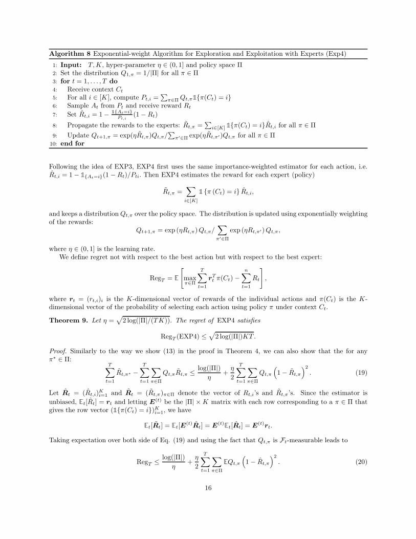
Algorithm 8 Exponential-weight Algorithm for Exploration and Exploitation with Experts (Exp4)

1: Input: T,K, hyper-parameter η ∈ (0, 1] and policy space Π2: Set the distribution Q1,π = 1/|Π| for all π ∈ Π3: for t = 1, . . . , T do4: Receive context Ct

5: For all i ∈ [K], compute Pt,i =∑

π∈ΠQt,π1π(Ct) = i6: Sample At from Pt and receive reward Rt

7: Set Rt,i = 1− 1At=iPt,i

(1−Rt)

8: Propagate the rewards to the experts: Rt,π =∑

i∈[K] 1π(Ct) = iRt,i for all π ∈ Π

9: Update Qt+1,π = exp(ηRt,π)Qt,π/∑

π′∈Π exp(ηRt,π′)Qt,π for all π ∈ Π10: end for

Following the idea of EXP3, EXP4 first uses the same importance-weighted estimator for each action, i.e.Rt,i = 1− 1At=i(1 −Rt)/Pti. Then EXP4 estimates the reward for each expert (policy)

Rt,π =∑

i∈[K]

1 π (Ct) = i Rt,i,

and keeps a distributionQt,π over the policy space. The distribution is updated using exponentially weightingof the rewards:

Qt+1,π = exp (ηRt,π)Qt,π/∑

π′∈Π

exp (ηRt,π′)Qt,π,

where η ∈ (0, 1] is the learning rate.We define regret not with respect to the best action but with respect to the best expert:

RegT = E

[maxπ∈Π

T∑

t=1

rTt π(Ct)−

n∑

t=1

Rt

],

where rt = (rt,i)i is the K-dimensional vector of rewards of the individual actions and π(Ct) is the K-dimensional vector of the probability of selecting each action using policy π under context Ct.

Theorem 9. Let η =√2 log(|Π|/(TK)). The regret of EXP4 satisfies

RegT (EXP4) ≤√2 log(|Π|)KT .

Proof. Similarly to the way we show (13) in the proof in Theorem 4, we can also show that the for anyπ∗ ∈ Π:

T∑

t=1

Rt,π∗ −T∑

t=1

∑

π∈Π

Qt,πRt,π ≤log(|Π|)

η+η

2

T∑

t=1

∑

π∈Π

Qt,π

(1− Rt,π

)2. (19)

Let Rt = (Rt,i)Ki=1 and Rt = (Rt,π)π∈Π denote the vector of Rt,i’s and Rt,π’s. Since the estimator is

unbiased, Et[Rt] = rt and letting E(t) be the |Π| ×K matrix with each row corresponding to a π ∈ Π that

gives the row vector (1π(Ct) = i)Ki=1, we have

Et[Rt] = Et[E(t)Rt] = E

(t)Et[Rt] = E

(t)rt.

Taking expectation over both side of Eq. (19) and using the fact that Qt,π is Ft-measurable leads to

RegT ≤log(|Π|)

η+η

2

T∑

t=1

∑

π∈Π

EQt,π

(1− Rt,π

)2. (20)

16

Let Yt,i = 1 − Rt,i, yt,i = 1 − rt,i and Yt,π = 1 − Rt,π for all i ∈ [K] and π ∈ Π. Define vectors Yt and Yt

similarly. Note that Yt = E(t)Yt and let At,i = 1At = i, which gives us Yt,i = At,iyt,i/Pt,i and

Et

[Y 2t,π

]= Et

(E

(t)π,At

yt,At

Pt,At

)2 =

K∑

i=1

(E

(t)π,iyt,i

)2

Pt,i≤

K∑

i=1

E(t)π,i

Pt,i.

Thus, by the definition of Pt,i,

E[∑

π∈Π

Qt,π(1− Rt,π)] ≤[∑

π∈Π

Qt,π

K∑

i=1

E(t)π,i

Pt,i

]= K.

Substituting into Eq. (20) gives us

RegT ≤log(|Π|)

η+ηTK

2≤√2TK log(|Π|),

when η =√2 log(|Π|)/(TK).

Now we take a look at the context space partition example introduced before. Assume we have a M -partition of the context space C. The regret bound is reduced from

√2|C| log(K)KT to

√2M log(K)KT

with the structural information.

2.2.3 Linear bandits and contextual linear bandits

One bandit per context method learns a distinct environment for each context, which fails when the contextspace is large or even infinite. Many healthcare applications, especially in mobile health, have continuouscontext including heart rate, sleeping time, etc. To model such applications with efficient algorithms, we needto assume some nice relationship between the context and environment. The simplest and most frequentlyused model of this kind is the contextual linear bandit.

Before we introduce the setting for contextual linear bandit, we first define linear bandit. In linear bandit,we do not directly model contexts but assume that the action space At ⊂ R

d (we will soon reveal the reasonbehind choosing a time varying action space) for some positive integer d, the reward on step t is sampledfrom a linear model:

Rt = 〈θ∗, At〉+ ηt, for some θ∗ ∈ Rd, (21)

and the noise ηt is usually assumed to be subgaussian. Note that, depending on the choice ofAt, linear banditscan subsume other bandit problems. For example, to capture the standard stochastic bandit environmentwith d actions, we set At = e1, . . . , ed for unit vectors (ei)i. Note that this choice of action set is not timevarying. The flexibility to choose time varying action sets is critical to capture contextual bandits. We simplylet At = ψ (Ct, i) ∈ R

d : i ∈ [K], for some known function ψ : C × [K] 7→ Rd. A common setup (Li et al.,

2010) considers one context per arm, where C ⊂ Rd×K and the function ψ(c, i) extracts the i-th column of

the matrix c. Another formulation assumes the same context ct ∈ Rd for every arm but assumes each arm

i has a parameter θ∗i ∈ Rd: Rt = 〈θ∗i , ct〉 + ηt, when arm i is chosen. Note that this is a special case of the

general formulation in (21). We can write θ∗ = (θ∗T1 , . . . , θ∗TK )T and At = (0d(i−1), CTt ,0d(K−i))Ki=1 ⊂ R

dK ,where 0n is the all-zero row vector of dimension n.

Linear Upper Confidence Bound (LinUCB). The regret for linear bandit is defined as

RegT = E[

T∑

t=1

maxat∈At

〈θ∗, at〉 −T∑

t=1

Rt].

17

Algorithm 9 Linear Upper Confidence Bound (LinUCB)

1: Input: δ, d, (At)t ⊂ Rd, (βt)t, λ.

2: for t = 1, . . . , T do3: Calculate θt using (22).

4: Compute the confidence set Θt = θ ∈ Rd : ‖θ − θt−1‖2Vt−1

≤ βt.5: Play At = argmaxa∈At

maxθ∈Θt〈θ, a〉.

6: Receive reward Rt and update Vt using (23).7: end for

We have seen UCB for the regular bandit environment as a powerful algorithm to balance the explorationand exploitation. In this section, we introduce a new UCB algorithm called LinUCB for linear bandit setting(Auer, 2002; Dani et al., 2008; Rusmevichientong and Tsitsiklis, 2010).

As the case in UCB, we follow the principle optimism in the face of uncertainty (OFU). Instead of directlybuilding confidence set over the mean function µa, we build confidence set Θt ⊂ R

d over the linear coefficientθ∗ that satisfies the following two properties: 1) Θt contains the optimal θ∗ with a high probability; 2) theset Θt should be as small as possible.

For that purpose, we consider the regularised least-square estimator up to step t,

θt = argminθ∈Rd

(t∑

s=1

(Rs − 〈θ, As〉)2 + λ‖θ‖22

), (22)

where λ > 0 is the penalty factor. Equ. (22) gives

θt = V −1t

t∑

s=1

AsRs, where V0 = λId and Vt = V0 +

t∑

s=1

AsA⊤s . (23)

Then the confidence set centering at θt is defined by

Θt+1 = θ ∈ Rd : ‖θ − θt‖2Vt

≤ βt+1, (24)

where (βt)t is an increasing sequence of constants that controls the level of confidence with β1 ≥ 1 as (Vt)talso have increasing eigenvalues. Lemma 10 shows the correctness of the confidence set defined in (24).LinUCB chooses actions that maximize the expected reward over all the possible θ’s in the confidence set.Details are given in Algorithm 9.

Lemma 10. Let δ ∈ (0, 1). Then, with a probability at least 1− δ, it holds that for all t ∈ N, θ∗ ∈ Θt definedin (24) with any sequence (βt)t satisfying

βt ≤√λ ‖θ∗‖2 +

√2 log

(1

δ

)+ d log

(detVtλd

).

Now using the confidence set in Lemma 10, we can show the following regret bound under some mildassumption on the boundedness of the action space. We refer reader to Part V of Lattimore and Szepesvári(2020) for the proof of Lemma 10.

Theorem 11. Assuming maxt∈[n] supa,b∈At〈θ∗, a− b〉 ≤ 1 and ‖a‖2 ≤ L for all a ∈ ⋃n

t=1At, using theconfidence set defined in Lemma 10, we have with a probability at least 1− δ, the expected regret of LinUCBis bounded by

RegT (LinUCB, ν) ≤ Cd√T log(L/δ), for some C > 0.

18

Proof. We first analyze the regret on each step. Let θt ∈ Θt be the parameter that maximize the expectedreward. Let A∗

t be the optimal action given context Ct. Then, using the fact that θ∗ ∈ Θt, we have〈θ∗, A∗

t 〉 ≤ 〈θ, At〉. Using Cauchy-Schwarz inequality, we have

rt = 〈θ∗, A∗t −At〉 ≤ 〈θt − θ∗, At〉 ≤ ‖At‖V −1

t−1

‖θt − θ∗‖Vt−1≤ 2‖At‖V −1

t−1

√βt.

Then the total regret is given by

RegT ≤T∑

t=1

2 ‖At‖V −1

t−1

√βt ≤

√√√√T

T∑

t=1

r2t ≤√TβT

∑

t=1

‖At‖2V −1

t−1

. (25)

Using the elliptical potential lemma (Carpentier et al., 2020),∑T

t=1

(1 ∧ ‖At‖2V −1

t−1

)≤ 2 log (detVT /detV0) .

The results follow by plugging this into (25) with the chosen βT and the fact that

det (VT ) =d∏

i=1

λi ≤(1

dtraceVT

)d

≤(traceV0 + TL2

d

)d

,

where λ1, . . . , λd are eigenvalues of Vt.

LinUCB gives a regret bound that scales with d. However, this is not the optimal rate when the actionset is finite. Auer (2002) proposed SupLinUCB which maintains a master algorithm that achieves a regretbound of

√dT log(TK) when the action space is finite.

LinUCB for contextual bandits. Chu et al. (2011) applied the LinUCB to the contextual bandit prob-lems. To be specific, they assume a context and a unknown parameter θ for each arm a and the reward isgenerated by

Rt = C⊤t,At

θ∗At+ ηt, where Ct,a, θ

∗a ∈ R

d.

Applying Theorem 11 gives us the regret bound of Kd√T . Li et al. (2010) showed a good performance of

the contextual bandit with LinUCB on News Article Recommendation task.

2.2.4 Sparse LinUCB

So far we have achieved regret bound of d√T log(T ), which scales linearly with d. However, the bound can

be vacuous for high-dimensional context (d≫ T ). Such high dimensional problems can occur in healthcareapplications. For example, Bastani and Bayati (2020) incorporates the high-dimensional genetic profile andmedical records with contextual bandits to design patient’s optimal medication dosage. Following the ideaof UCB, the key is to construct a confidence set that accounts for the sparsity. To tackle the problem, weintroduce a powerful tool that converts online prediction problem to confidence set estimation, with whicha UCB-style algorithm can be designed using any online predicting method and we can analyze its regret ina unified way.

Online to Confidence Set Conversion. There is a conversion from the online prediction to confidencesets. We consider online linear regression problem with a squared loss, which has been well-explored in thepast decade (Huang et al., 2008; Javanmard and Montanari, 2014). The agent interacts with the environmentin the following manner where in each round t:

1. The environment chooses a context Ct ∈ R and At ∈ Rd in an arbitrary way.

2. The value of At is revealed to the agent.

19

Algorithm 10 Online linear predictor UCB

1: Input: δ ∈ (0, 1), an online predictor with a regret bound Bt

2: for t = 1, . . . , T do3: Receive action set At

4: Compute the confidence set Θt using (26)5: Play At = argmaxa∈At

maxθ∈Θt〈θ, a〉 and receive reward Rt

6: Feed At to the online linear predictor and obtain prediction Rt

7: Feed Rt and loss to the linear predictor as feedback.8: end for

3. The agent generate a prediction Rt.

4. The environment reveals Rt to the agent as well as the loss (Rt − Rt)2.

The regret of an agent with respective to the best linear predictor is given by

ρT =

T∑

t=1

(Rt − Rt)2 − inf

θ⊂Rd

T∑

t=1

(Rt − 〈θ, At〉)2.

Theorem 12 (Online-to-Confidence-Set Conversion (Abbasi-Yadkori et al., 2012)). Let δ ∈ (0, 1) and as-sume that θ∗ ∈ Θ, noise ηt’s are R-sub-Gaussian and ρt ≤ Bt. Let

βt(δ) = 1 + 2Bt + 32R2 log

(R√8 +√1 +Bt

δ

).

Then

Θt+1 =

θ ∈ R

d :

t∑

s=1

(Rs − 〈θ, As〉)2 ≤ βt(δ), (26)

satisfies P(θ∗ ∈ Θt+1∀t ∈ N) ≥ 1− δ.Theorem 12 provides a tool for constructing confidence set for the prediction of any online learning

algorithm with a regret guarantee. One can develop the Online linear predictor UCB (OLR-UCB) as shownin Algorithm 10.

Let ‖θ∗‖2 ≤ m2. Using Theorem 12 and the standard regret decomposition for UCB-style algorithm, onecan show the following regret bound:

RT ≤√8dT (m2

2 + βT−1(δ)) log

(1 +

T

d

).

Application to sparse online linear prediction. Note that our goal is to derive a regret bound witha lower dependency on the ambient dimension d. In the standard regression problem, learnability of high-dimensional data relies on the sparsity assumption which assumes the number of non-zero dimensions is lessor equal to a positive integer s.

Assumption 1. (sparse parameter) The true parameter θ∗ satisfies ‖θ∗‖0 ≤ s for some s > 0.

To this end, we adopt SeqSEW (Gerchinovitz, 2011) as the online linear prediction algorithm, whichachieves the online learning regret ρT = O(s log(T )). Combined with Theorem 12, we have the followingresult:

Theorem 13. With a high probability, the we bound the regret of OLR-UCB with SeqSEW as the onlinepredictor by

RegT = O(√dsT ). (27)

20

This improves over the d√T by LinUCB in the previous section when s ≪ d. As pointed out by

Lattimore and Szepesvári (2020), for any algorithm, there exists an infinite action space such that RegT =Ω(√dsT ). Thus, the bound in (27) is minimax optimal. Despite its optimality, our result still have the

unavoidable dependence of√d. Bastani and Bayati (2020) derived a regret bound of O(K(s log(d) log(T ))2),

when the action set is finite. More variants of high-dimensional sparse linear bandits are discussed inHao et al. (2020).

2.3 Offline Learning

So far we have been discussing bandit problems in the online learning setting, where we are free to chooseactions while collecting the dataset. In many real applications, collecting data in the online manner can beexpensive and can cost a lot of time. In such situations we might want to evaluate a target policy using alarge but fixed dataset that has been collected for years by a different policy. This setting is called offlinelearning.

Given a fixed contextual bandit environment, the value of a policy is defined as vπ = Eat∼π(ct)rt Formally,offline bandits, also referred as off-policy evaluation aims at evaluating the value vπ of a new policy usinga sequence of interactions ST = (ct, at, rt)

Tt=1, where ct, at and rt are the context, action and reward

respectively at step t. The actions are chosen by the data-generating policy πD, which is also referred asbehavior policy or logging policy. In this section,

One solution is to learn the reward and context distribution using a parametric or non-parametric methodand then evaluate the new policy with the simulator by sampling context and rewards from the learntdistribution. Although this approach is straightforward, the modeling step is often very expensive anddifficult, and more importantly, it often introduces modeling bias to the simulator, making it hard to justifyreliability of the obtained evaluation results.

Li et al. (2011) proposed a simple algorithm (Algorithm 11) that uses an unbiased estimator of thepolicy value when the behavior policy picks arms uniformly at random. The method is to simply use all theinteractions in the dataset that coincide with the action that the policy being evaluated would have taken.They show that vπ is an unbiased estimator of vπ and with a high probability (vπ−vπ)2 = O (Kvπ/n) , wherevπ is the true expected value of the policy as defined above. They also successfully applied the off-policyevaluation to the News Article Recommendation system. Mary et al. (2014) improved upon Algorithm 11via bootstrapping techniques. They give a bootstrapped estimator for any quantile of the distribution of theestimated value vπ that allows some evaluation of the uncertainty.

Algorithm 11 Policy Evaluator

1: Input: a policy π; stream of interactions ST of length T2: h0 ← ∅, Vπ ← 0 and N ← 03: for t = 1, . . . , T do4: Get the i-th interaction (ci, ai, rt) from ST

5: if π(ht−1, ct) = at then6: ht ← ht−1 ∪ (ct, at, rt)7: Vπ ← Vπ + rt and N ← N + 18: end if9: end for

10: Output: vπ = Vπ/N

Minimax rate lower bound. To understand how good our algorithms perform, we start with establishinga minimax lower bound that characterizes the inherent hardness of the off-policy value estimation problem.Let Rmax, σ ∈ R

+. Define the class of reward distributions V(σ,Rmax) with bounded mean and variance as

V(σ,Rmax) := ν = (Pa,c)a,c∈A×C : 0 ≤ ER∼Pa,c[R] ≤ Rmax and Var[R | a, c] ≤ σ2, ∀a, c ∈ A× C.

21

Any estimator v is a function that maps (π, πD, ST ) to an estimate of vπ. Let the context C ∼ λ with adensity relative to Lebesgue measure. The minimax rate is defined as

Mn(π, λ, πD , σ, Rmax) := infv

supν∈V(σ,Rmax)

E[(v(π, πD, ST )− vπ)2],

where the expectation is taken over the distribution of the dataset ST that depends on (π, λ, πD).A critical value that determines the hardness of the problem is

V1 := EC∼λ,A∼πD(·,C)

[π2(A,C)/π2

D(A,C)].

Wang et al. (2017) (Corollary 1) gives the following lower bound for Rn:

Mn(π, λ, πD, σ, Rmax) ≥V1(σ

2 +R2max)

700T. (28)

Importance sampling estimator. Wang et al. (2017) give some analysis on the minimax rate of the off-policy evaluation given a known data-generating policy, denoted by πD. We slightly abuse the notation andlet π(a, c) denote the probability of choose a using policy π under the context c. They consider ImportanceSampling (IS) estimator (Charles et al., 2013) and Weighted Importance Sampling (WIS) estimator givenby

vIS,π =1

T

T∑

t=1

π(at, ct)

πD(at, ct)rt and vWIS,π =

T∑

t=1

π(at,ct)πD(at,ct)∑T

t′=1π(at′ ,ct)πD(at′ ,ct)

rt, respectively.

It is shown in Dudík et al. (2014) that the IS estimator is unbiased and it achieves the minimax ratein (28) when n is sufficiently large. The WIS estimator is biased with a lower variance. It also enjoys theminimax optimality up to a logarithmic constant.

Regression estimator. Another common method, so called regression estimator or plug-in estimator,simply learns the reward distribution and plugs it in. Let r : A×C 7→ R is an estimator for the mean reward.The regression estimator is given by

vReg,π :=1

T

T∑

t=1

∑

a

π(a, ct)r(a, ct).

When the context space and action space are finite. One can use the simple sample average estimatorr(a, c) = (

∑Tt=1 1(at = a, ct = c)ri)/(

∑Tt=1 1(at = a, ct = c)). Interestingly, one can write the regression

estimator using sample average as

vReg =1

T

T∑

t=1

π (at, ct)

πD (at, ct)rt, where πD (a, c) =

∑t 1(at = a, ct = c)

T.

There is a strong connection between IS and regression estimator. That is regression estimator simplyreplaces the πD with its empirical estimator. Regression estimator is biased while its variance is normallylower than IS (Dudík et al., 2011; Li et al., 2015). Regression estimator is also shown to be minimax optimalwhen n is sufficiently large. The simple plugin method using sample average is not applicable when contextspace is infinite. When more information on how rewards depend on contexts and actions, we can posit aparametric or non-parametric model of E[R | C,A] and fit it to obtain an estimator. Due to the difficultiesof having a good estimation x, which may suffer model-misspecification or high variance, pure regressionestimator only works well in problem with finite actions. For more details, we refer reader to a more recentpaper (Kim et al., 2021).

22

Doubly robust estimator. Based on the above discussions about IS and Regression Estimator, it isnatural to combine the both. Doubly Robust (DR) (Bang and Robins, 2005; Dudík et al., 2011; Jiang and Li,2016) which is a combination of regression and IS estimator, and can achieve the low variance of regressionand no (or low) bias of IS. The method is named by Doubly Robust because it is accurate if at least one ofthe estimator is accurate. DR estimator is defined as

vDR =1

T

∑

t

[π(at, ct)

πD(at, ct)(rt − r(at, ct)) +

∑

a

π(a, ct)r(a, ct)

].

Informally, the estimator uses r(a, c) as a baseline and corrects the baseline when the action more likelyto be sampled from the target policy. DR enjoys both the low variance of Regression estimator and thelow bias of the IS estimator and also matches the minimax lower bound in 28. Wang et al. (2017) furtherintroduces the SWITCH estimator that takes account into the scale of the importance weight. When theimportance weight is large, it switches to the regression estimator, which significantly reduces the variancewhile introducing only little bias. It performs better in the numerical experiments.

Non-asymptotic regime. All of the above estimators achieve minimax optimality when n is sufficientlylarge. Ma et al. (2021) discussed regime when the sample size is not large. They showed that there is afundamental statistical gap between algorithm with and without the knowledge of the behavior policy in thisregime. They proposed a competitive ratio that measures the MSE of an algorithm with unknown behaviorpolicy relative to the lower bound of all algorithms with known behavior policy. Competitive ratio is alwaysgreater than 1. A competitive ratio closer to 1 indicates that the algorithm can performance as good asthe algorithm with known behavior policy. Ma et al. (2021) showed that regression estimator has minimaxoptimal competitive ratio of the rate is O(K), where K is the number of actions. That means an algorithmwithout the knowledge of the behavior policy has to pay multiplicative factor of K compared to that withthe knowledge.

3 Advanced Topics

We now review a selection of advanced topics in bandit algorithms that are relevant to applications inhealthcare.

3.1 Non-stationarity

We have discussed two basic and extreme cases of bandit theory: stochastic bandit models and adversarialbandit models. In the former, the reward distribution for every arm is static whereas in the latter, it canchange arbitrarily over time. In this section, we describe a more practical setting that sits in the “middle” ofabove two extreme models: non-stationary bandits. Specifically, the reward distributions change over time,but the amount of changes cannot be as arbitrary as the adversarial setting.

For a non-stationary multi-armed bandit environment ν, we define the reward mean for arm a at time tby µa,t(ν) or µa,t for simplicity. Then the dynamic regret is

RegT =

T∑

t=1

maxa

µa,t − E

[T∑

t=1

µAt,t

].

Unlike the regret definition for the adversarial setting that is with respect to the best single arm, dynamicregret is defined with respect to the sequence of best arms at each time step. There are two popularconstraints that quantify the reward changes. One is the total count of changes in the mean reward thatoccur before time T :

ST = 1 +

T∑

t=2

1µa,t−1 6= µa,t, for some a.

23

Settings where the above quantity is assumed to be small are also called piece-wise stationary. Anotherconstraint quantifies the total variation for the reward mean:

BT =

T∑

t=2

maxa|µa,t − µa,t−1|.

Piecewise Stationary Setting. The first algorithm designed for the non-stationary MAB under finitenumber of reward mean changes is Exp3.S (Auer et al., 2002), which is a variant of the Exp3 algorithm. Theexpected regret of Exp3.S is O(ST

√KT log(KT )) in general, but can be improved to O(

√STKT log(KT ))

if ST is used to tune the algorithm parameters. Later on, Garivier and Moulines (2011) proved that nopolicy can achieve problem-dependent regret smaller than O(

√T ) in the non-stationary case, and Exp3.S

is thus optimal up to logarithmic factors of T . Garivier and Moulines (2011) also studied two UCB-basedalgorithms: discounted UCB (D-UCB) which was first proposed by Kocsis and Szepesvári (2006) and sliding-window UCB (SW-UCB). Their main idea is to encourage using more recent data in UCB reward estimations.When S is given, both algorithms achieve O(K

√ST logT ) regret. Another body of works explore the idea

of monitoring the reward distributions by change-detection methods and reset the bandit algorithm ac-cordingly. Using this idea, Monitored-UCB (M-UCB) (Cao et al., 2019) combines the UCB algorithm witha change-point detection component based on running sample means over a sliding window and achievesO(√KST logT ) regret under certain assumption on the reward mean change. In same year, Auer et al.

(2019) proposed an action elimination algorithm ADSWITCH that again detects changes in the mean re-ward and restarts the learning algorithm accordingly. Without knowing S nor making other assumptions,ADSWITCH achieves O(

√KST logT ) regret.

Bounded Total Variation Setting. Comparing with piecewise stationary setting, bounded total varia-tion is a softer constraint. Here nature has the power to change the reward at every round but only up to a to-tal amount limit BT . Besbes et al. (2014) proposed the Rexp3 policy that uses the famous Exp3 algorithm asa subroutine and restarts it at every batch. Rexp3 with a batch size tuned by BT has O((BTK logK)1/3T 2/3)regret that nearly matches the lower bound of Ω(KBT )

1/3T 2/3) in this setting (Besbes et al., 2014).The non-stationary setup has also studied in linear bandits and contextual bandits. We briefly describe

the latter one as an example. Define the distribution of the context-reward pairs C × [0, 1]K by D1, . . . ,DT .At each round, the environment samples (ct, xt) and reveals ct to the agent, then the agent picks an armAt ∈ [K] and observes xt(At). For a fixed set of policies Π that contains mappings: C → [K], the dynamicregret is defined as:

RegT =T∑

t=1

maxπ∈Π

E(c,x)∼Dt[x(π(c))] −

T∑

t=1

xt(At).

Similar to the MAB setting, there are two ways to measure the non-stationary of the environment: totalnumber of changes and the total variation in below.

S = 1 +T∑

t=2

1Dt 6= Dt−1,

BT =

T∑

t=2

‖Dt −Dt−1‖TV .

Chen et al. (2019) proposed ADA-ILTCB+ algorithm that is parameter-free, efficient and achieves optimal

regret O(min√K(log |Π|)ST ,

√K(log |Π|)T + (K log |Π|BT )

1/3T 2/3) by randomly entering replay phasesto detect non-stationarity. More recently, a generic reduction has been studied that allows one to convertcertain algorithms for the stationary setting into algorithms for the non-stationary setting (Wei and Luo,2021). What is nice about this work is that the resulting algorithms often simultaneously achieve optimalguarantees in terms of both S and BT without prior knowledge of any of these parameters.

24

3.2 Robustness

So far, we have discussed stochastic and adversarial bandits. Stochastic bandit is an ideal setting, since itassumes a fixed reward distribution. Adversarial, on the other hand, considers a too extreme scenario. Inreal-world applications, some of the observed rewards may be corrupted resulting in deviation from purelystochastic behavior. For instance, there might be clerical errors while creating electronic health records orsensor errors in recording health status from wearable devices. If the reward is self-reported by patients, therecan be corruptions due to mistakes, lack of attention, boredom, etc. In this section, we consider algorithmsthat are robust to possible corruptions. Note that this setting is between purely stochastic and adversarialbut in a different way than the non-stationary bandit discussed in Section 3.1.

Fraction corruption model. The fraction corruption model limits the fraction of the total number ofrounds that an adversarial corruption can happen. Assume corruptions happen with a probability η ∈ [0, 1].The adversary closely follows the progress of arm pulling and reward generation. At each time step t, afterthe algorithm has decided to pull an arm At, the adversary first decides whether to corrupt this arm pullor not by performing a Bernoulli trail Zt ∈ 0, 1 with a mean η ∈ [0, 1]. Then it generates a corruption ζarbitrarily. After this, the “clean reward” R∗

t is generated by the environment. The reward a player receivesat step t is

Rt = 1Zt = 0R∗t + 1Zt = 1ζt.

Since the rewards may be contaminated, directly running the algorithms built for stochastic bandits canresult in degraded performance. Several papers have proposed variants of UCB that use a more robustestimate. Kapoor et al. (2019) proposed RUCB-TUNE (Robust UCB) which makes two crucial changesto the classical UCB: RUCB-TUNE uses the median and a tuned variance estimate instead of the simplesample mean and variance to construct its upper bound. The algorithm requires an upper bound η0 on thecorruption rate η. Their analyses are built on the environment with Gaussian reward distributions and theyhave a regret bound of O((1 − η)

√KT log(T ) + η0(µ

∗ +B)T ), where B is an upper bound on the scales ofcorruptions |ζt| and µ∗ is the maximum expected reward of all the arms. They provide another algorithmRUCB with a similar result. RUCB does not require the knowledge of η0 but it requires an upper bound onthe variance of rewards for all the arms.

Niss and Tewari (2020) considers a stronger requirement that all the arms have no more than η-fractionof corruptions. They proposed crUCB (contamination robust-UCB), which mimics RUCB in the generalframework. The only difference is that they allow a variety of robust mean estimates including α-trimmedmean, mean estimates that ignores the largest (1−α)-fraction of data, α-shorth mean. Their algorithms areevaluated by uncontaminated regrets, the regret between true rewards of the best possible actions and thealgorithm-chosen actions:

RegT = maxa∈A

E[

T∑

t=1

R∗a(t)−R∗

At(t)],

If the contamination fraction is small enough, both crUCB using α-shorth mean and α-trimmed mean achieveuncontaminated regret of

√KT log(T )+

∑a ∆a, where ∆a is the gap between the expected reward of a and

the optimal action.

Budget-bounded corruption model. In budget-bounded corruption model (Lykouris et al., 2018), allthe rounds can be possibly corrupted but the total deviation between the “clean rewards” and the corruptedrewards is bounded. We define the total corruption budget as

BT =

T∑

t=1

‖R∗t −Rt‖.

Gupta et al. (2019) proposed BARBAR (Bandit Algorithm with Robustness: Bad Arms get Recourse) basedon the arm elimination algorithm discussed in Section 2 with some crucial modifications that make it robust

25

to corruptions. Gupta et al. (2019) show that their algorithm achieves a gap-dependent regret bound of

RegT = O

KBT +

∑

a 6=a⋆

log T

∆alog

(K

δlogT

) .

without knowing the value of C.

3.3 Dealing with Constraints

In standard bandit settings, the only criterion to evaluate the performance of an algorithm is the regret (eithercumulative or simple regret). In this section, we introduce constrained bandit problems, where the agentalso needs to satisfy certain constraints while minimizing its regret. Depending on the actual problem’sdemands, different types of constraints have been considered. For healthcare applications, two types ofconstraints frequently arise in practice. First, delivering an intervention might consume resources such asdoctor’s time, patient’s attention, phone battery and power, etc. We might therefore want to maximizerewards subject to a budget on resource consumption. Second, we might be worried that uncontrolledexploration might yield performance that is substantially worse than an existing standard of care. Withthese concerns in mind, in this section we consider the following two settings: bandits with knapsacks andconservative bandits.

Bandits with Knapsacks (BwK). The name of bandits with knapsacks comes from the well-knownknapsack problem in combinatorial optimization that studies packing items into a fixed-size knapsack. In aknapsack problem, each item has its value and size. Its ultimate goal is to fill the knapsack with as large valueas possible. The bandits with knapsacks then focus on a stochastic online version of the knapsack problem.Many practical scenarios can be captured by this framework. For example, in medical trials, physicians maybe limited by the cost of treatment materials while optimizing the health condition of the patients. In onlinerecommendations, the website designer may be constrained by the advertisers’ budgets while maximizingits profit. We follow the terminologies and notations in Badanidiyuru et al. (2018) to formally describe thissetting and their proposed algorithms.

An agent is given an action set A and there are d resources being consumed. At every round, the agentselects an action At ∈ A and observes a reward Xt along with a d-dimensional resource consumption vectorct. For each resource i ∈ [d], the total consumption should not exceed the pre-specified budget Bi at anyround. The agent stops immediately when the total consumption of certain resource exceeds its budget.Denote the stopping time by τ , the goal is to maximize the total reward until time τ . The worst-case regretfor an algorithm is defined as the difference between the benchmark total reward OPT4 and the algorithm’sexpected total reward until τ .

To solve the problem, Badanidiyuru et al. (2018) proposed two algorithms. The first one is a primal-dualalgorithm called PrimalDualBwK. At every round, it estimates the upper confidence bound for the expectedreward and the lower confidence bound for the resource consumption for each arm. Then PrimalDualBwKplays the most “cost-effective” arm, i.e., the one with highest ratio of the expected reward’s upper bound

to the expected cost. The regret of PrimalDualBwK is proved to be O(√|A|OPT+OPT

√|A|/B

), where

B := miniBi. Note that without the resource constraints, the regret bound becomes O(√|A|OPT

)=

O(√|A|T

)that is optimal up to logarithmic factors since the only constraint is the time horizon T and we

can simply set B = T in the general regret formula. The second algorithm is called BalancedExploration.Its design principle is to explore as much as possible while avoiding obviously sub-optimal strategies. They

show that the regret of BalancedExploration is O(√

d|A|OPT+OPT√d|A|/B

). Even though its regret

4An optimal dynamic policy that maximizes the expected total reward given prior knowledge on all latent distributions suchas the reward distribution and the cost consumption for each action.

26

has worse dependence on d comparing with PrimalDualBwK, BalancedExploration performs better in somespecial cases.

Comparing with the general constraint in above knapsack framework, researchers have also consideredmore specific settings. For example, other than the time horizon, there is a single resource with deterministicconsumption and different arms consume the resource at different rates (Tran-Thanh et al., 2010, 2012;Ding et al., 2013; Xia et al., 2015; Zhou and Tomlin, 2018). Such problems are often called budgeted bandits.Agrawal and Devanur (2014) generalized the BwK model by allowing arbitrary concave rewards and convexconstraints. Furthermore, similar constrained bandit problems are also studied in settings that includescontextual bandits (Agrawal and Devanur, 2014; Wu et al., 2015; Agrawal and Devanur, 2016) and evenadversarial bandits (Sun et al., 2017; Immorlica et al., 2019).

Conservative Bandits. It is well-known that standard bandit algorithms often explore wildly in theirearly stages, so their regret over initial rounds can be very high. However, safety is one of the crucial concernsfor designing adaptive experiments, so the early stage high regret cannot be tolerated in some high stakesscenarios. For instance, the UCB algorithm can assign treatments almost randomly to a patient during thefirst several rounds, which may cause severe problems for the patient’s overall health. A company may alsonot be able to withstand the extremely low revenue initially if its operation is in great need of cash flow. Inthese examples, the real situation is that the physician or the company already have their favorite policiesthat operate well. They would like to explore new strategies to optimize their treatment performance orrevenue while maintaining their performance to not be significantly worse than a baseline, uniformly overtime. Conservative bandits (Wu et al., 2016) exactly model this problem. We follow their terminology andnotation to describe the problem framework.

We use 0, 1, . . . ,K as the indices of actions, in which the arm indexed by 0 correspond to the defaultaction (the agent’s typical strategy) and the other arms are the alternatives to be explored. The agentselects an arm At ∈ 0, 1, . . . ,K in round t. Denote Rt,i as the random reward received at time t after

playing arm i, then the regret and pseudo-regret are defined as RegT = maxi∈0,1,...,K

∑Tt=1Rt,i − Rt,At

and RegT = maxi∈0,1,...,K

∑Tt=1 µi − µAt

. To ensure that the agent performs as good as his or her usualstrategy, the algorithm needs to satisfy:

t∑

s=1

Rs,As≥ (1− α)

t∑

s=1

Rs,0, (29)

where 0 < α ≤ 1. Above constraint guarantees that the reward collected by the agent is at least (1 − α)fraction of the reward from simply playing arm 0. The objective of conservative bandits algorithms is tominimize regret while satisfying (29) for all t. To solve the problem, (Wu et al., 2016) proposed a novelalgorithm called conservative UCB which is based on UCB with the novel twist of maintaining (29) beingsatisfied. Basically, the agent follows the UCB suggestion if (29) can be satisfied from their estimation,otherwise, the agent switches to the conservative arm 0. They show that conservative UCB achieves pseudo-

regret RegT = O(√KT + K

αµ0), where µ0 denotes the expected reward for arm 0. For more details, including

gap-dependent regret and regret analysis for the adversarial setting, we refer the reader to Wu et al. (2016).The concept of conservative bandits, namely performing as good as a baseline uniformly over time,

is quite general. Recently, it has been generalized to more settings, e.g., conservative contextual ban-dits (Kazerouni et al., 2016; Garcelon et al., 2020b) and conservative reinforcement learning (Garcelon et al.,2020a).

3.4 Fairness

Algorithmic fairness has become an increasingly important topic in machine learning research (Barocas et al.,2021). Fairness is also a concern in healthcare applications due to the biases in data collection and algo-rithmic design (Paulus and Kent, 2020). Using healthcare cost as a proxy for healthcare needs leads tobiased risk scores that hurt Black patients (Obermeyer et al., 2019). Using genetic datasets collected mostly

27

from patients of European ancestry leads to biased genetic risk scores on patients with non-European an-cestries (Martin et al., 2019). Unfairness can also be rooted in algorithmic design. Algorithms that simplymaximizing user responses can be unfair in how they allocate exposure to the items in recommendationsystems (Singh and Joachims, 2018). In this section, we review several popular definitions of fairness inbandit literature and discuss how to calibrate unfairness.

Two types of fairness. Though there remains little agreement about what “fairness” should mean indifferent contexts, the literature can be divided into two broad families: those that target group fairnessand those that target individual fairness. Group fairness requires the algorithm to maintain fairness acrossdifferent demographic groups (say by race or gender) that are supposed to be treated equally. As wementioned above, biased healthcare algorithms may hurt patients from certain demographic groups due tolow representative. Individual fairness, on the other hand, asks for some constraints on the individual level,including two slightly different types: fairness through awareness, which requires that similar individuals betreated similarly and meritocratic fairness, which requires that less qualified individuals not be favored overmore qualified individuals. Individual fairness in healthcare is also important: for two patients with similardemographic information or physical condition, we shall not develop an algorithm that performs much betterfor one patient while useless (or even harmful) for the other.

In the context of bandits, the literature can be further divided into those that model individuals as armsin the MAB setting and those that models individuals as contexts in the contextual bandits setting. We givesome examples of fairness definitions from each category.

Individual fairness. We start from individual fairness in the MAB setting with each arm representing anindividual. Joseph et al. (2016) proposed the use of meritocratic fairness. Formally, an algorithm is said tobe δ-fair if over T time steps, , for any pair of arms a, a′, and any round t,

πt(a) > πt(a′) only if µa > µa′

with probability at least 1 − δ. This requires the algorithm to give equal probability to choose two armsunless one there is strong evidence that µa > µa′ . Joseph et al. (2016) developed an algorithm that is δ-fair based on the traditional UCB algorithm. In specific, they maintain a set of arms that chains to thearm with highest UCB. All the arms in the set are given the same probability to be selected. Their regret

bound is O(√K3T ln TK

δ ), with a higher cubic dependence on K, which is the price they pay to give equal

probability to all the arms in the set. More generally, Liu et al. (2017) considers a fairness through awareness.An algorithm is said to be (ǫ1, ǫ2, δ)-smooth fair 5, if for any pair of arms a, a′ and any t, with a probabilityat least 1− δ,

|πt(a)− πt(a′)| ≤ ǫ1|µa − µa′ |+ ǫ2.

They introduced a fairness regret to quantify the violation that occurs when the arm with the highest rewardrealization at a given time is not selected with the highest probability. Formally, they have

RegT =

T∑

t=1

E

[K∑

i=1

maxP ∗(i)− πt(i), 0],

where P ∗(i) is the probability that arm i has the highest regret. They developed a modified ThompsonSampling algorithm with an initial uniform exploration phase that achieve fairness regret of O((KT )2/3).Wang et al. (2021) also aims at the fairness through awareness by comparing to the optimal fair policy π∗,

π∗(a)

π∗(a′)=

f(µa)

f(µa′)for some metric function f.

5Note that Liu et al. (2017) considers a general divergence function for the distribution of action selection and rewards, weintroduce a special case here for a cleaner form.

28

They in turn target at the fairness regret, the cumulative L0 norm of π∗ − πt. Other individual fairnessdefinition that simply requires a minimum number of pulls for each arms is considered by Patil et al. (2020)and Chen et al. (2020).

Group fairness. For group fairness, one may divide arms into n groups G1, . . . , Gn. Schumann et al.(2019) proposed an algorithm ensuring that the probability of pulling an arm does not change based ongroup membership:

P(pull a | a ∈ Gi) = P(pull a | a ∈ Gj), ∀i, j < n and a ∈ A.In other words, one cannot prefer one arm over the other one based on the group information.

Some literature treats each context ct as an individual and aims at the fairness among different contexts.(Huang et al., 2020) divides the context space into two groups, a privileged group G+ and a protected groupG−. A group-level cumulative mean reward is defined as

RG =1

|TG|∑

t∈TG

Rt, where TG is the set of all rounds with gt in group G.

Their group fairness requires that |E[RG+ − RG−

]| ≤ τ , where τ ∈ R+ reflects the tolerance degree of

unfairness. Assuming a linear bandit setting, they proposed a Fair-LinUCB algorithm, that penalize thearms that are unfair by decreasing the corresponding UCB values.

Counterfactual fairness. Another line of work (Kusner et al., 2017) models fairness through causal in-ference. Their fairness definition is normally referred to as Counterfactual Fairness. In the group fairness, werequire the distributions of the value of interest are the same across different demographic groups. However,what we really want is that the demographic group information does not cause the unfairness, which can notbe fully inferred from the group fairness definition. Counterfactual fairness, on the other hand, requires thedistribution of the value of interest does not change when the demographic group were changed from one tothe other while keeping all the other context variable unchanged.

General fairness metric. All the above methods requires certain fairness definition, it is natural to askwhether there is an universal algorithm that adapts to various fairness definition. In real-applications, wemay not know the exact form of fairness metric. Instead, we may know whether certain policy violatesfairness condition. Instead of studying a specific fairness metric, Gillen et al. (2018) developed an algorithmthat achieves fairness through a fairness oracle, which tells the algorithm whether fairness is violated. Thisalso allows great flexibility in the choice of fairness metric. At each round, each arm i ∈ [K] is given acontext Ct,i ∈ R

d. The probability of selecting action i at the step t is denoted by πt,i, which is a vectordenoting the probability of selecting . We denote the vector of context (policy) at round t by ct (πt). Thefairness oracle is define as following. Intuitively, it tells the algorithm, which pairs of actions violate thefairness metric.

Definition 4. Let ∆([K]) be the set of all distributions over [K]. Given a user-specified distance functiond, a fairness oracle Od is a function Od : R

d×K ×∆([K])→ 2[K]×[K], defined such that

Od (ct, πt) = (i, j) : |πt,i − πt,j | > d (Ct,i, Ct,j) .

They developed an algorithm that only has access to the fairness oracle. The algorithm has the numberof fairness violations depending only logarithmically on T and a regret bound of the optimal rate O(

√T )

with respect to the best fair policy.

3.5 Benefiting from Causal Knowledge

Causal bandit is an example of a structured bandit problem where actions are composed of interventionson variables of a causal graph. According to the underlying causal dynamics, performing an intervention

29

can help learn another intervention’s reward distribution. Algorithms for causal bandit problems exploit thecausal dependency among interventions to reduce the regret or sample complexity.

Bareinboim et al. (2015) was the first to connect bandit problems with causal models. One of the mainissues that make causal inference hard is the existence of confounders defined below, which can confusecorrelation and causation. Bareinboim et al. (2015) pointed out the importance of capturing the confoundersbefore actually performing actions. In particular, they proposed a new criterion for choosing actions calledregret decision criterion (RDC). Under RDC rule, the agent collects her intention (includes informationon confounders) on selecting actions and re-thinks based on the estimated reward statistics for the currentintention and then decides which action to play. Since the actual selected action can be different than theagent’s intention, the agent decides in a counterfactual way.

Definition 5 (Confounder). A confounder is a variable that influences both the dependent variable andindependent variable.

Later on, Lattimore et al. (2016) formally proposed the causal bandit framework via causal graphs. Acausal model consists of a directed acyclic graph G over a set of random variables V = V1, . . . , Vn and ajoint distribution P that factorizes over G. A size m hard intervention (action) is denoted by do(V = v),which assigns the values v = v1, . . . , vm ⊂ V to the corresponding variables V = V1, . . . , Vm. In causalbandits, the action set is defined as

A := do(V = v)|V ⊂ V ,v ∈ Dom(V),

or its subset and the optimal intervention is a∗ := argmaxa∈A E[R|a].Many practical problems can be modeled via above framework. For example, in healthcare applications,

the physician adjusts several features such as dose levels on different medicines or life-style advices to achievesome desirable clinical outcomes (Liu et al., 2020). Genetic engineering also involves direct manipulationof genes using biotechnology to produce improved organisms. In these problems, the number of interven-tions can be exponentially large in the number of manipulable variables so that standard MAB algorithmscannot work efficiently. To address this issue, recent work on causal bandits has developed methods thatexploit causal information to achieve simple or cumulative regret that does not scale with the number ofinterventions (Lattimore et al., 2016; Sen et al., 2017; Lee and Bareinboim, 2018; Lu et al., 2020, 2021a).We summarize existing methodologies below.

Refining the Policy Space. Assuming the causal graph is known (confounders may also exist), Lee and Bareinboim(2018) proposed an intervention set reduction algorithm. They showed that not all interventions are worth-while to be played, because there are equivalences among interventions and some interventions can beproved to be no better than others. Their algorithm filters out redundant interventions using the causalgraph structure before applying any standard MAB algorithm on the reduced intervention set, also calledpossibly-optimal minimal intervention set (POMIS). Since the size of POMIS is usually much smaller than|A|, the corresponding regret can be reduced. Follow-up work in Lee and Bareinboim (2019) further showedthat the expected reward for interventions in a POMIS can be estimated from each other in certain cases.Their method also works well when some variables are non-manipulable. We remark that the step of findingthe POMIS solely relies on the given causal graph structure and does not involve performing any intervention.

Accelerating Using Causal Graph Side Information in Standard MAB Algorithms. Recall thata key step in bandit algorithm is estimating the expected reward for each arm µa. Intuitively speaking,one needs to play each arm for enough number of times in order to get accurate estimations if interventionsare independent. But in causal bandits, interventions are correlated with each other so that performing oneintervention can help with estimating others according to the shared causal model. Lattimore et al. (2016)studied the best arm identification problem via importance weighting. Their algorithm achieves simpleregret O(

√m/T ), where m can be smaller than |A| in many scenarios. Sen et al. (2017) further generalized

the algorithm in Lattimore et al. (2016) to a soft intervention setting and proved gap-dependent regretguarantees. In soft interventions, the agent does not directly set values to specific variables, but instead

30

change their conditional probabilities given their direct parents. Lu et al. (2020) proposed causal UCB andcausal TS algorithms that achieve O(

√ZT ) cumulative regret, where Z is a graph dependent number and

can be exponentially smaller than |A|. A causal linear bandit framework and its efficient algorithms werealso well studied. Furthermore, gap-dependent worst-case regret bound and a budgeted causal bandit settingwas also considered in follow-up works (Nair et al., 2021).

3.6 Multi-task Learning

Multitask learning is the learning paradigm in machine learning that aims at leveraging information in multi-ple tasks to achieve a better sample efficiency by solving them jointly rather than separately (Zhang and Yang,2021). Multitask learning algorithms usually assume some similarity between tasks that allows informationsharing. In the context of multitask bandit, each bandit is called a task and various similarity assumptionson the reward distribution can be made. This can model many interesting scenarios. For instance, a groupof patient with the same disease can be seen as multiple tasks. We can not directly use the same policy, as apersonalized treatment should be applied to each patient. However, some patients’ responses may be similarto the other’s such that one can transfer the information across patients. Recall that we use ν = (Pa, a ∈ A)denote a bandit instance. A general multitask bandit framework can be summarized below:

Given a set of bandits ν1, . . . , νn, Discrepancy(νi, νj) is small for some i, j ∈ [n],

for some discrepancy measure on bandit instances.In this subsection, we will review some interesting works on multitask bandit and compare their assump-

tions on discrepancy and the corresponding regret bounds. We will also cover the potential applications ofmultitask bandits.

Parametric Model. Early work on multitask bandit was done by Cesa-Bianchi et al. (2013) who consid-ered a gang of contextual bandits connected with a graph V,E, where V = 1, . . . , n is the node set andE is the edge set. Each node i is assumed to be a linear bandit with rewards generated by Ri(c) = θTi c+ǫi(c)given a context c, where ǫi(c) is a conditionally zero-mean noise. Any two nodes that are adjacent on thegraph have low discrepancy compared to the total scale:

∑i∈V ‖θi‖2 ≫

∑(i,j)∈E ‖θi − θj‖2. Their discrep-

ancy measure is simply the L2 distance on the unknown parameters. However, their analysis only shows abenefit of a factor n in the logarithmic term. In the literature of supervised multitask learning, the benefitcould be a factor of n1/2 outside the logarithmic term (Maurer et al., 2016). Another property makes it hardfor their algorithm to generalize to other settings is that the discrepancy information on tasks similaritiesis partially known to the agent through the graph structure. Generally speaking, the agent does not knowwhich tasks are similar and have to adaptively learn the information.

As an improvement, Gentile et al. (2014); Li et al. (2016) consider an unknown graph with clusteredstructure, and all the bandits within the same cluster share a common reward distribution, which is alsofrom a linear model. The algorithm is to simply cluster the bandits based on the feedbacks and pool the datafrom all the bandits from the same cluster. Instead of have a dependency of n as for the baseline algorithmthat learns all the bandit separately, their regret is O(dm

√T ), where m≪ n is the number of clusters.

Non-parametric Model. Despite the encouraging results by Gentile et al. (2014); Li et al. (2016), theclustered structure and linear payoffs are strong assumptions. Deshmukh et al. (2017) proposed a kernelregression model that allows general similarities. Formally, they assume the reward is generated by meanfunction f : Z × C 7→ R, where Z is called the task similarity space, C is the context from the context spaceC. Let k be a SPD (semi-positive definite) kernel on Z × C with the form

k ((z, c), (z′, c′)) = kZ (z, z′) kC (c, c′) ,

where kZ and kC are SPD kernels on Z = 1, . . . , n representing n tasks and C. They assume that f isfrom the RKHS, Hk corresponding to k. Kernel kZ characterized the similarity between different bandits,for instance:

31

1. Independent: kZ(z, z′) = 1z=z′ , i.e. observations from different tasks are not sharing any information.

2. Pooled: kZ ≡ 1, i.e all the observations from different tasks are treated the same.

3. Multi-task: kZ is a PDS matrix reflecting task similarity.

Their algorithm KMTL-UCB gives an regret bound of O(√Trzrc), where rz is the rank of the n × nmatrix KZ = [kZ (zi, zi)]

ni=1 and rc is the rank of KCT

:= [kC(cat,t, cat′ ,t′)]Tt,t′=1. To compare, the regular

regret bound of learning one task independently is O(√Trc) and all tasks independently gives O(n√Trc).The scaling of rz determines the benefits of multitask learning: rz = n corresponds to the first case above withkZ(z, z

′) = 1z=z′ and rz = 1 corresponds to the second case with kZ ≡ 1. Though Deshmukh et al. (2017)gives a general way to characterize the multitask bandit benefits, their algorithm still relies on the knowledgeof the similarity kernel kZ . In practice, one can learn a kernel, but little theory has been established to justifythis practice.

Adaptive Learning. Tomkins et al. (2021) proposed Intelligent Pooling, a generalization of a Thompsonsampling contextual bandit for learning personalized treatment policies. They assume the reward for useri ∈ [n] is generated by

Ri = φ(Ci, Ai)T θi + ǫi,

where φ : C ×A 7→ Rd is the pre-specified mapping from contexts and actions and θi ∈ R

d is the personalizedparameter to learn. IntelligentPooling imposes each wi as a random-effects upon a population-level parameterwpop, i.e. wi = wpop + ui with ui the Gaussian random effect. Prior distribution of wpop is also assumed tobe Gaussian. IntelligentPooling runs by sampling wi,t from the posterior distribution of wi. The algorithmuses random effects to adaptively pool users’ data based on the degree to which users exhibit heterogeneousrewards that is away from the population behavior (wpop). They showed a regret bound of O(dn

√T ).

4 Conclusion

We reviewed basic topics in bandit algorithms that are helpful in understanding their increasing role inmobile health, and more broadly, precision medicine. We also discussed a selection of advanced topics thatmight inform the design of the next generation of bandit driven mobile health applications. We hope thatthe reader has gained an appreciation of the beauty and power of bandit algorithms and of their relevanceto mobile health and precision medicine. However, like any methodology, bandit algorithms do have theirlimitations. First, bandit algorithms assume that an appropriate reward is available upfront. In practice,especially in healthcare applications, the design of rewards to be optimized is a difficult problem with noeasy solution. The issues involved in specified a reward function that is aligned with the goals of varioushuman stakeholders have been brought into focus more recently under the term ”the alignment problem”(Christian, 2020). Second, bandit algorithms do not take into account delayed impacts of the agent’s actions.When actions have delayed impacts, it might be beneficial to take an action with low immediate reward if itincreases the probability of higher rewards later on. The full treatment of this problem of delayed impact ofactions requires techniques from reinforcement learning (Sutton and Barto, 2018). In fact, bandit problemscan be thought of as the simplest of reinforcement learning problems.

References

Abbasi-Yadkori, Y., Pál, D., and Szepesvári, C. (2011). Improved algorithms for linear stochastic bandits.Advances in neural information processing systems, 24:2312–2320.

Abbasi-Yadkori, Y., Pal, D., and Szepesvari, C. (2012). Online-to-confidence-set conversions and applicationto sparse stochastic bandits. In Artificial Intelligence and Statistics, pages 1–9. PMLR.

32

Agrawal, S. and Devanur, N. (2016). Linear contextual bandits with knapsacks. Advances in Neural Infor-mation Processing Systems, 29:3450–3458.

Agrawal, S. and Devanur, N. R. (2014). Bandits with concave rewards and convex knapsacks. In Proceedingsof the fifteenth ACM conference on Economics and computation, pages 989–1006.

Agrawal, S. and Goyal, N. (2012). Analysis of thompson sampling for the multi-armed bandit problem. InConference on learning theory, pages 39–1. JMLR Workshop and Conference Proceedings.

Agrawal, S. and Goyal, N. (2013). Further optimal regret bounds for thompson sampling. In Artificialintelligence and statistics, pages 99–107. PMLR.

Aguilera, A., Figueroa, C. A., Hernandez-Ramos, R., Sarkar, U., Cemballi, A., Gomez-Pathak, L., Mira-montes, J., Yom-Tov, E., Chakraborty, B., Yan, X., et al. (2020). mhealth app using machine learning toincrease physical activity in diabetes and depression: clinical trial protocol for the diamante study. BMJopen, 10(8):e034723.

Ameko, M. K., Beltzer, M. L., Cai, L., Boukhechba, M., Teachman, B. A., and Barnes, L. E. (2020). Offlinecontextual multi-armed bandits for mobile health interventions: A case study on emotion regulation. InFourteenth ACM Conference on Recommender Systems, pages 249–258.

Audibert, J.-Y., Bubeck, S., et al. (2009). Minimax policies for adversarial and stochastic bandits. In COLT,volume 7, pages 1–122.

Auer, P. (2002). Using confidence bounds for exploitation-exploration trade-offs. Journal of Machine Learn-ing Research, 3(Nov):397–422.

Auer, P., Cesa-Bianchi, N., Freund, Y., and Schapire, R. E. (2002). The nonstochastic multiarmed banditproblem. SIAM journal on computing, 32(1):48–77.

Auer, P., Gajane, P., and Ortner, R. (2019). Adaptively tracking the best bandit arm with an unknownnumber of distribution changes. In Conference on Learning Theory, pages 138–158. PMLR.

Auer, P. and Ortner, R. (2010). Ucb revisited: Improved regret bounds for the stochastic multi-armed banditproblem. Periodica Mathematica Hungarica, 61(1-2):55–65.

Badanidiyuru, A., Kleinberg, R., and Slivkins, A. (2018). Bandits with knapsacks. Journal of the ACM(JACM), 65(3):1–55.

Bang, H. and Robins, J. M. (2005). Doubly robust estimation in missing data and causal inference models.Biometrics, 61(4):962–973.

Bareinboim, E., Forney, A., and Pearl, J. (2015). Bandits with unobserved confounders: A causal approach.Advances in Neural Information Processing Systems, 28:1342–1350.

Barocas, S., Hardt, M., and Narayanan, A. (2021). Fairness and Machine Learning. fairmlbook.org.http://www.fairmlbook.org.

Bastani, H. and Bayati, M. (2020). Online decision making with high-dimensional covariates. OperationsResearch, 68(1):276–294.

Besbes, O., Gur, Y., and Zeevi, A. (2014). Stochastic multi-armed-bandit problem with non-stationaryrewards. Advances in neural information processing systems, 27:199–207.

Bubeck, S., Munos, R., and Stoltz, G. (2009). Pure exploration in multi-armed bandits problems. InInternational conference on Algorithmic learning theory, pages 23–37. Springer.

33

Cao, Y., Wen, Z., Kveton, B., and Xie, Y. (2019). Nearly optimal adaptive procedure with change detec-tion for piecewise-stationary bandit. In The 22nd International Conference on Artificial Intelligence andStatistics, pages 418–427. PMLR.

Carpentier, A., Vernade, C., and Abbasi-Yadkori, Y. (2020). The elliptical potential lemma revisited. arXivpreprint arXiv:2010.10182.

Cesa-Bianchi, N., Gentile, C., and Zappella, G. (2013). A gang of bandits. In Proceedings of the 26thInternational Conference on Neural Information Processing Systems-Volume 1, pages 737–745.

Cesa-Bianchi, N. and Lugosi, G. (2012). Combinatorial bandits. Journal of Computer and System Sciences,78(5):1404–1422.

Charles, D., Chickering, M., and Simard, P. (2013). Counterfactual reasoning and learning systems: Theexample of computational advertising. Journal of Machine Learning Research, 14.

Chen, Y., Cuellar, A., Luo, H., Modi, J., Nemlekar, H., and Nikolaidis, S. (2020). The fair contextual multi-armed bandit. In Proceedings of the 19th International Conference on Autonomous Agents and MultiAgentSystems, pages 1810–1812.

Chen, Y., Lee, C.-W., Luo, H., and Wei, C.-Y. (2019). A new algorithm for non-stationary contextualbandits: Efficient, optimal and parameter-free. In Conference on Learning Theory, pages 696–726. PMLR.

Christian, B. (2020). The Alignment Problem: Machine Learning and Human Values. W. W. Norton.

Chu, W., Li, L., Reyzin, L., and Schapire, R. (2011). Contextual bandits with linear payoff functions.In Proceedings of the Fourteenth International Conference on Artificial Intelligence and Statistics, pages208–214. JMLR Workshop and Conference Proceedings.

Clayton, M. K. (1989). Covariate models for bernoulli bandits. Sequential Analysis, 8(4):405–426.

Dani, V., Hayes, T. P., and Kakade, S. M. (2008). Stochastic linear optimization under bandit feedback.

Deshmukh, A. A., Dogan, U., and Scott, C. (2017). Multi-task learning for contextual bandits. arXivpreprint arXiv:1705.08618.

Ding, W., Qin, T., Zhang, X.-D., and Liu, T.-Y. (2013). Multi-armed bandit with budget constraint andvariable costs. In Proceedings of the AAAI Conference on Artificial Intelligence, volume 27.

Dudík, M., Erhan, D., Langford, J., and Li, L. (2014). Doubly robust policy evaluation and optimization.Statistical Science, 29(4):485–511.

Dudík, M., Langford, J., and Li, L. (2011). Doubly robust policy evaluation and learning. arXiv preprintarXiv:1103.4601.

Even-Dar, E., Mannor, S., Mansour, Y., and Mahadevan, S. (2006). Action elimination and stoppingconditions for the multi-armed bandit and reinforcement learning problems. Journal of machine learningresearch, 7(6).

Forman, E. M., Kerrigan, S. G., Butryn, M. L., Juarascio, A. S., Manasse, S. M., Ontañón, S., Dallal, D. H.,Crochiere, R. J., and Moskow, D. (2019). Can the artificial intelligence technique of reinforcement learninguse continuously-monitored digital data to optimize treatment for weight loss? Journal of behavioralmedicine, 42(2):276–290.

Garcelon, E., Ghavamzadeh, M., Lazaric, A., and Pirotta, M. (2020a). Conservative exploration in rein-forcement learning. In International Conference on Artificial Intelligence and Statistics, pages 1431–1441.PMLR.

34

Garcelon, E., Ghavamzadeh, M., Lazaric, A., and Pirotta, M. (2020b). Improved algorithms for conservativeexploration in bandits. In Proceedings of the AAAI Conference on Artificial Intelligence, volume 34, pages3962–3969.

Garivier, A. and Moulines, E. (2011). On upper-confidence bound policies for switching bandit problems. InInternational Conference on Algorithmic Learning Theory, pages 174–188. Springer.

Gentile, C., Li, S., and Zappella, G. (2014). Online clustering of bandits. In International Conference onMachine Learning, pages 757–765. PMLR.

Gerchinovitz, S. (2011). Sparsity regret bounds for individual sequences in online linear regression. InProceedings of the 24th Annual Conference on Learning Theory, pages 377–396. JMLR Workshop andConference Proceedings.

Gillen, S., Jung, C., Kearns, M., and Roth, A. (2018). Online learning with an unknown fairness metric.arXiv preprint arXiv:1802.06936.

Goldenshluger, A. and Zeevi, A. (2011). A note on performance limitations in bandit problems with sideinformation. IEEE transactions on information theory, 57(3):1707–1713.

Goldenshluger, A. and Zeevi, A. (2013). A linear response bandit problem. Stochastic Systems, 3(1):230–261.

Gupta, A., Koren, T., and Talwar, K. (2019). Better algorithms for stochastic bandits with adversarialcorruptions. In Conference on Learning Theory, pages 1562–1578. PMLR.

Hao, B., Lattimore, T., and Wang, M. (2020). High-dimensional sparse linear bandits. arXiv preprintarXiv:2011.04020.

Haussler, D. and Warmuth, M. (2018). The probably approximately correct (pac) and other learning models.The Mathematics of Generalization, pages 17–36.

Huang, J., Ma, S., and Zhang, C.-H. (2008). Adaptive lasso for sparse high-dimensional regression models.Statistica Sinica, pages 1603–1618.

Huang, W., Labille, K., Wu, X., Lee, D., and Heffernan, N. (2020). Achieving user-side fairness in contextualbandits. arXiv preprint arXiv:2010.12102.

Immorlica, N., Sankararaman, K. A., Schapire, R., and Slivkins, A. (2019). Adversarial bandits with knap-sacks. In 2019 IEEE 60th Annual Symposium on Foundations of Computer Science (FOCS), pages 202–219.IEEE.

Javanmard, A. and Montanari, A. (2014). Confidence intervals and hypothesis testing for high-dimensionalregression. The Journal of Machine Learning Research, 15(1):2869–2909.

Jiang, N. and Li, L. (2016). Doubly robust off-policy value evaluation for reinforcement learning. In Inter-national Conference on Machine Learning, pages 652–661. PMLR.

Jin, T., Xu, P., Shi, J., Xiao, X., and Gu, Q. (2020). Mots: Minimax optimal thompson sampling. arXivpreprint arXiv:2003.01803.

Jin, Y., Yang, Z., and Wang, Z. (2021). Is pessimism provably efficient for offline rl? In InternationalConference on Machine Learning, pages 5084–5096. PMLR.

Joseph, M., Kearns, M., Morgenstern, J., and Roth, A. (2016). Fairness in learning: Classic and contextualbandits. arXiv preprint arXiv:1605.07139.

Kapoor, S., Patel, K. K., and Kar, P. (2019). Corruption-tolerant bandit learning. Machine Learning,108(4):687–715.

35

Kaufmann, E., Korda, N., and Munos, R. (2012). Thompson sampling: An asymptotically optimal finite-timeanalysis. In International conference on algorithmic learning theory, pages 199–213. Springer.

Kazerouni, A., Ghavamzadeh, M., Abbasi-Yadkori, Y., and Van Roy, B. (2016). Conservative contextuallinear bandits. arXiv preprint arXiv:1611.06426.

Kim, W., Kim, G.-s., and Paik, M. C. (2021). Doubly robust thompson sampling for linear payoffs. arXivpreprint arXiv:2102.01229.

Klasnja, P., Hekler, E. B., Shiffman, S., Boruvka, A., Almirall, D., Tewari, A., and Murphy, S. A. (2015).Microrandomized trials: An experimental design for developing just-in-time adaptive interventions. HealthPsychology, 34(S):1220.

Kocsis, L. and Szepesvári, C. (2006). Discounted ucb. In 2nd PASCAL Challenges Workshop, volume 2.

Konstantinidou, M. K., Karaglani, M., Panagopoulou, M., Fiska, A., and Chatzaki, E. (2017). Are the originsof precision medicine found in the corpus hippocraticum? Molecular diagnosis & therapy, 21(6):601–606.

Kusner, M. J., Loftus, J. R., Russell, C., and Silva, R. (2017). Counterfactual fairness. arXiv preprintarXiv:1703.06856.

Lai, T. L. and Robbins, H. (1985). Asymptotically efficient adaptive allocation rules. Advances in appliedmathematics, 6(1):4–22.

Langford, J. and Zhang, T. (2007). Epoch-greedy algorithm for multi-armed bandits with side information.Advances in Neural Information Processing Systems (NIPS 2007), 20:1.

Lattimore, F., Lattimore, T., and Reid, M. D. (2016). Causal bandits: Learning good interventions viacausal inference. arXiv preprint arXiv:1606.03203.

Lattimore, T. (2015). Optimally confident ucb: Improved regret for finite-armed bandits. arXiv preprintarXiv:1507.07880.

Lattimore, T. (2018). Refining the confidence level for optimistic bandit strategies. The Journal of MachineLearning Research, 19(1):765–796.

Lattimore, T. and Szepesvári, C. (2020). Bandit algorithms. Cambridge University Press.

Lee, S. and Bareinboim, E. (2018). Structural causal bandits: where to intervene? Advances in NeuralInformation Processing Systems 31, 31.

Lee, S. and Bareinboim, E. (2019). Structural causal bandits with non-manipulable variables. In Proceedingsof the AAAI Conference on Artificial Intelligence, volume 33, pages 4164–4172.

Lei, H., Nahum-Shani, I., Lynch, K., Oslin, D., and Murphy, S. A. (2012). A" smart" design for buildingindividualized treatment sequences. Annual review of clinical psychology, 8:21–48.

Li, L., Chu, W., Langford, J., and Schapire, R. E. (2010). A contextual-bandit approach to personalizednews article recommendation. In Proceedings of the 19th international conference on World wide web,pages 661–670.

Li, L., Chu, W., Langford, J., and Wang, X. (2011). Unbiased offline evaluation of contextual-bandit-basednews article recommendation algorithms. In Proceedings of the fourth ACM international conference onWeb search and data mining, pages 297–306.

Li, L., Munos, R., and Szepesvári, C. (2015). Toward minimax off-policy value estimation. In ArtificialIntelligence and Statistics, pages 608–616. PMLR.

36

Li, S., Karatzoglou, A., and Gentile, C. (2016). Collaborative filtering bandits. In Proceedings of the 39thInternational ACM SIGIR conference on Research and Development in Information Retrieval, pages 539–548.

Liao, P., Greenewald, K., Klasnja, P., and Murphy, S. (2020). Personalized heartsteps: A reinforcement learn-ing algorithm for optimizing physical activity. Proceedings of the ACM on Interactive, Mobile, Wearableand Ubiquitous Technologies, 4(1):1–22.

Liu, S., See, K. C., Ngiam, K. Y., Celi, L. A., Sun, X., and Feng, M. (2020). Reinforcement learning forclinical decision support in critical care: comprehensive review. Journal of medical Internet research,22(7):e18477.

Liu, Y., Radanovic, G., Dimitrakakis, C., Mandal, D., and Parkes, D. C. (2017). Calibrated fairness inbandits. arXiv preprint arXiv:1707.01875.

Lu, Y., Meisami, A., and Tewari, A. (2021a). Causal bandits with unknown graph structure. arXiv preprintarXiv:2106.02988.

Lu, Y., Meisami, A., and Tewari, A. (2021b). Low-rank generalized linear bandit problems. In InternationalConference on Artificial Intelligence and Statistics, pages 460–468. PMLR.

Lu, Y., Meisami, A., Tewari, A., and Yan, W. (2020). Regret analysis of bandit problems with causalbackground knowledge. In Conference on Uncertainty in Artificial Intelligence, pages 141–150. PMLR.

Lykouris, T., Mirrokni, V., and Paes Leme, R. (2018). Stochastic bandits robust to adversarial corruptions.In Proceedings of the 50th Annual ACM SIGACT Symposium on Theory of Computing, pages 114–122.

Ma, C., Zhu, B., Jiao, J., and Wainwright, M. J. (2021). Minimax off-policy evaluation for multi-armedbandits. arXiv preprint arXiv:2101.07781.

Martin, A. R., Kanai, M., Kamatani, Y., Okada, Y., Neale, B. M., and Daly, M. J. (2019). Clinical use ofcurrent polygenic risk scores may exacerbate health disparities. Nature genetics, 51(4):584–591.

Mary, J., Preux, P., and Nicol, O. (2014). Improving offline evaluation of contextual bandit algorithms viabootstrapping techniques. In International Conference on Machine Learning, pages 172–180. PMLR.

Maurer, A., Pontil, M., and Romera-Paredes, B. (2016). The benefit of multitask representation learning.Journal of Machine Learning Research, 17(81):1–32.

Nair, V., Patil, V., and Sinha, G. (2021). Budgeted and non-budgeted causal bandits. In InternationalConference on Artificial Intelligence and Statistics, pages 2017–2025. PMLR.

Neu, G. (2015). Explore no more: Improved high-probability regret bounds for non-stochastic bandits. arXivpreprint arXiv:1506.03271.

Niss, L. and Tewari, A. (2020). What you see may not be what you get: Ucb bandit algorithms robust tovarepsilon-contamination. In Conference on Uncertainty in Artificial Intelligence, pages 450–459. PMLR.

Obermeyer, Z., Powers, B., Vogeli, C., and Mullainathan, S. (2019). Dissecting racial bias in an algorithmused to manage the health of populations. Science, 366(6464):447–453.

Paredes, P., Gilad-Bachrach, R., Czerwinski, M., Roseway, A., Rowan, K., and Hernandez, J. (2014).Poptherapy: Coping with stress through pop-culture. In Proceedings of the 8th International Confer-ence on Pervasive Computing Technologies for Healthcare, pages 109–117.

Patil, V., Ghalme, G., Nair, V., and Narahari, Y. (2020). Achieving fairness in the stochastic multi-armedbandit problem. In Proceedings of the AAAI Conference on Artificial Intelligence, volume 34, pages5379–5386.

37

Paulus, J. K. and Kent, D. M. (2020). Predictably unequal: understanding and addressing concerns thatalgorithmic clinical prediction may increase health disparities. NPJ digital medicine, 3(1):1–8.

Piette, J. D., Farris, K. B., Newman, S., An, L., Sussman, J., and Singh, S. (2015). The potential impact ofintelligent systems for mobile health self-management support: Monte carlo simulations of text messagesupport for medication adherence. Annals of Behavioral Medicine, 49(1):84–94.

Piette, J. D., Krein, S. L., Striplin, D., Marinec, N., Kerns, R. D., Farris, K. B., Singh, S., An, L., and Heapy,A. A. (2016). Patient-centered pain care using artificial intelligence and mobile health tools: protocol for arandomized study funded by the us department of veterans affairs health services research and developmentprogram. JMIR research protocols, 5(2):e53.

Rabbi, M., Aung, M. H., Zhang, M., and Choudhury, T. (2015). Mybehavior: automatic personalizedhealth feedback from user behaviors and preferences using smartphones. In Proceedings of the 2015 ACMInternational Joint Conference on Pervasive and Ubiquitous Computing, pages 707–718.

Rabbi, M., Klasnja, P., Choudhury, T., Tewari, A., and Murphy, S. (2019). Optimizing mhealth interventionswith a bandit. In Baumeister, H. and Montag, C., editors, Mobile Sensing and Digital Phenotyping: NewDevelopments in Psychoinformatics. Springer.

Rindtorff, N. T., Lu, M., Patel, N. A., Zheng, H., and D’Amour, A. (2019). A biologically plausiblebenchmark for contextual bandit algorithms in precision oncology using in vitro data. arXiv preprintarXiv:1911.04389.

Rusmevichientong, P. and Tsitsiklis, J. N. (2010). Linearly parameterized bandits. Mathematics of OperationsResearch, 35(2):395–411.

Sarkar, J. (1991). One-armed bandit problems with covariates. The Annals of Statistics, pages 1978–2002.

Schumann, C., Lang, Z., Mattei, N., and Dickerson, J. P. (2019). Group fairness in bandit arm selection.arXiv preprint arXiv:1912.03802.

Sen, R., Shanmugam, K., Dimakis, A. G., and Shakkottai, S. (2017). Identifying best interventions throughonline importance sampling. In International Conference on Machine Learning, pages 3057–3066. PMLR.

Shrestha, S. and Jain, S. (2021). A bayesian-bandit adaptive design for n-of-1 clinical trials. Statistics inMedicine, 40(7):1825–1844.

Singh, A. and Joachims, T. (2018). Fairness of exposure in rankings. In Proceedings of the 24th ACMSIGKDD International Conference on Knowledge Discovery & Data Mining, pages 2219–2228.

Sun, W., Dey, D., and Kapoor, A. (2017). Safety-aware algorithms for adversarial contextual bandit. InInternational Conference on Machine Learning, pages 3280–3288. PMLR.

Sutton, R. S. and Barto, A. G. (2018). Reinforcement learning: An introduction. MIT press.

Tewari, A. and Murphy, S. A. (2017). From ads to interventions: Contextual bandits in mobile health.In Rehg, J., Murphy, S. A., and Kumar, S., editors, Mobile Health: Sensors, Analytic Methods, andApplications. Springer.

Thompson, W. R. (1933). On the likelihood that one unknown probability exceeds another in view of theevidence of two samples. Biometrika, 25(3/4):285–294.

Tomkins, S., Liao, P., Klasnja, P., and Murphy, S. (2021). Intelligentpooling: practical thompson samplingfor mhealth. Machine Learning, pages 1–43.

38

Tran-Thanh, L., Chapman, A., De Cote, E. M., Rogers, A., and Jennings, N. R. (2010). Epsilon–first policiesfor budget–limited multi-armed bandits. In Proceedings of the AAAI Conference on Artificial Intelligence,volume 24.

Tran-Thanh, L., Chapman, A., Rogers, A., and Jennings, N. (2012). Knapsack based optimal policies forbudget–limited multi–armed bandits. In Proceedings of the AAAI Conference on Artificial Intelligence,volume 26.

Wang, C.-C., Kulkarni, S. R., and Poor, H. V. (2005). Arbitrary side observations in bandit problems.Advances in Applied Mathematics, 34(4):903–938.

Wang, L., Bai, Y., Sun, W., and Joachims, T. (2021). Fairness of exposure in stochastic bandits. arXivpreprint arXiv:2103.02735.

Wang, Y.-X., Agarwal, A., and Dudık, M. (2017). Optimal and adaptive off-policy evaluation in contextualbandits. In International Conference on Machine Learning, pages 3589–3597. PMLR.

Wei, C.-Y. and Luo, H. (2021). Non-stationary reinforcement learning without prior knowledge: An optimalblack-box approach. arXiv preprint arXiv:2102.05406.

Wu, H., Srikant, R., Liu, X., and Jiang, C. (2015). Algorithms with logarithmic or sublinear regret forconstrained contextual bandits. arXiv preprint arXiv:1504.06937.

Wu, Y., Shariff, R., Lattimore, T., and Szepesvári, C. (2016). Conservative bandits. In InternationalConference on Machine Learning, pages 1254–1262. PMLR.

Xia, Y., Li, H., Qin, T., Yu, N., and Liu, T.-Y. (2015). Thompson sampling for budgeted multi-armedbandits. In Proceedings of the 24th International Conference on Artificial Intelligence, pages 3960–3966.

Yang, Y., Zhu, D., et al. (2002). Randomized allocation with nonparametric estimation for a multi-armedbandit problem with covariates. The Annals of Statistics, 30(1):100–121.

Yao, J., Brunskill, E., Pan, W., Murphy, S., and Doshi-Velez, F. (2020). Power-constrained bandits. arXivpreprint arXiv:2004.06230.

Yom-Tov, E., Feraru, G., Kozdoba, M., Mannor, S., Tennenholtz, M., and Hochberg, I. (2017). Encouragingphysical activity in patients with diabetes: intervention using a reinforcement learning system. Journal ofmedical Internet research, 19(10):e338.

Zhang, K. W., Janson, L., and Murphy, S. A. (2021). Statistical inference with m-estimators on bandit data.arXiv preprint arXiv:2104.14074.

Zhang, Y. and Yang, Q. (2021). A survey on multi-task learning. IEEE Transactions on Knowledge andData Engineering.

Zhou, D. and Tomlin, C. (2018). Budget-constrained multi-armed bandits with multiple plays. In Proceedingsof the AAAI Conference on Artificial Intelligence, volume 32.

Zhou, Z., Wang, Y., Mamani, H., and Coffey, D. G. (2019). How do tumor cytogenetics inform cancertreatments? dynamic risk stratification and precision medicine using multi-armed bandits. Dynamic RiskStratification and Precision Medicine Using Multi-armed Bandits (June 17, 2019).

39