Department of Quantitative Methods & Information Systems ... · Department of Quantitative Methods...

Business Statistics

Department of Quantitative Methods & Information Systems

Dr. Mohammad Zainal QMIS 220

Chapter 12

Chi-square test of independence

& Analysis of Variance

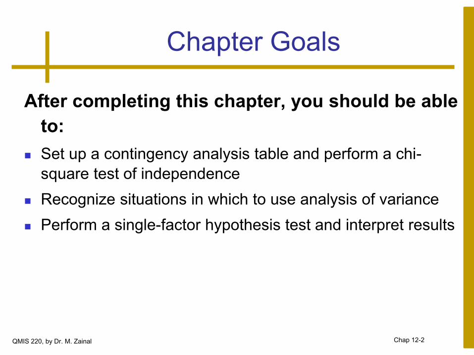
Chapter Goals

After completing this chapter, you should be able

to:

Set up a contingency analysis table and perform a chi-

square test of independence

Recognize situations in which to use analysis of variance

Perform a single-factor hypothesis test and interpret results

QMIS 220, by Dr. M. Zainal Chap 12-2

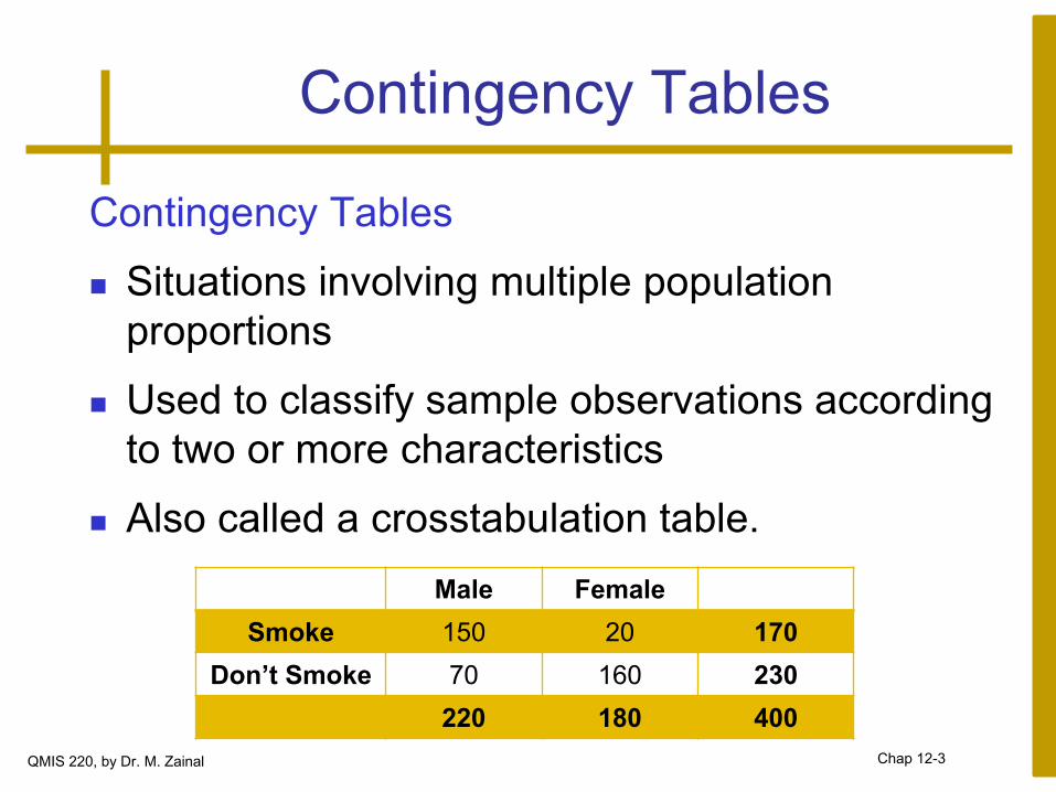
Contingency Tables

Contingency Tables

Situations involving multiple population

proportions

Used to classify sample observations according

to two or more characteristics

Also called a crosstabulation table.

Male Female

Smoke 150 20 170

Don’t Smoke 70 160 230

220 180 400


Contingency Tables

It can be of any size: 2x3, 3x2, 3x3, or 4x2

The first digit refers to the number of rows, and

the second refers to the number of columns.

In general, R × C table contains R rows and C

columns.

The number of cells in a contingency table is

obtained by multiplying the number of rows by

the number of columns.


Contingency Tables

We may want to know if there is an association

between being a male or female and smoking

or not.

The null hypothesis that the two characteristics

of the elements of a given population are not

related (independent)

Against the alternative hypothesis that the two

characteristics are related (dependent).

Degrees of freedom for the test are:

df = (R-1)(C-1) QMIS 220, by Dr. M. Zainal Chap 12-5

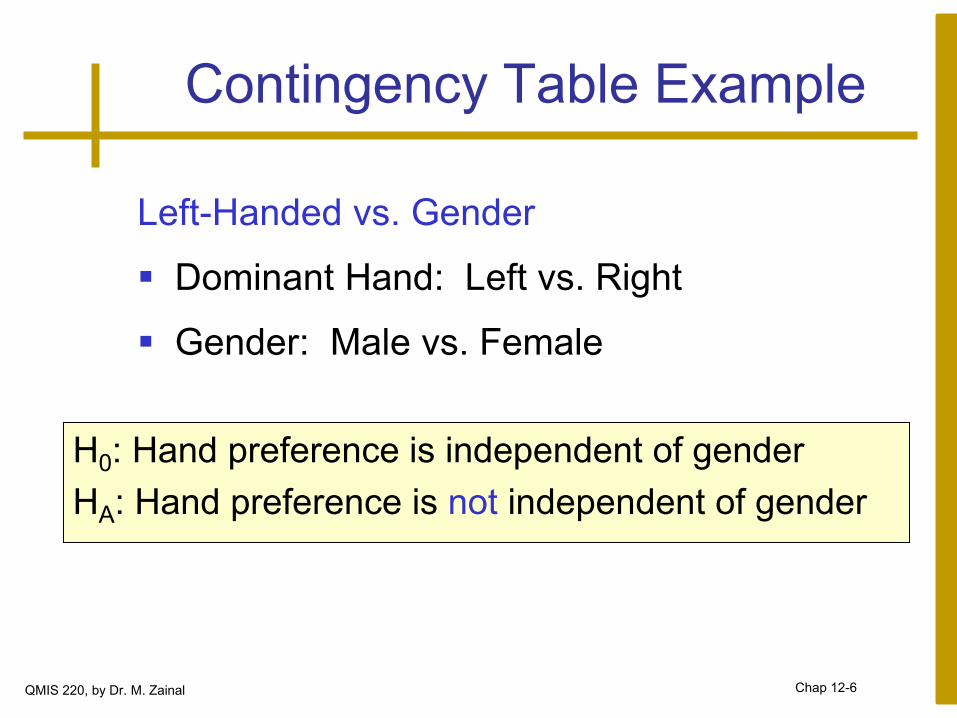
Contingency Table Example

H0: Hand preference is independent of gender

HA: Hand preference is not independent of gender

Left-Handed vs. Gender

Dominant Hand: Left vs. Right

Gender: Male vs. Female


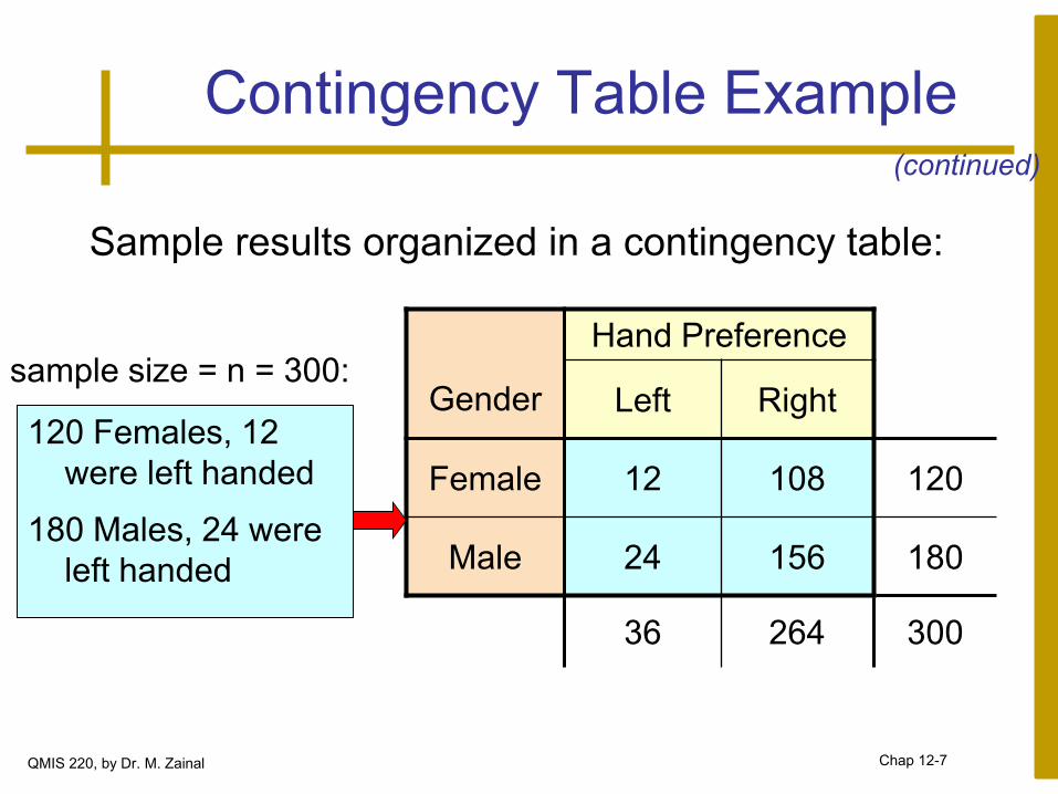
Contingency Table Example

Sample results organized in a contingency table:

(continued)

Gender

Hand Preference

Left Right

Female 12 108 120

Male 24 156 180

36 264 300

120 Females, 12

were left handed

180 Males, 24 were

left handed

sample size = n = 300:


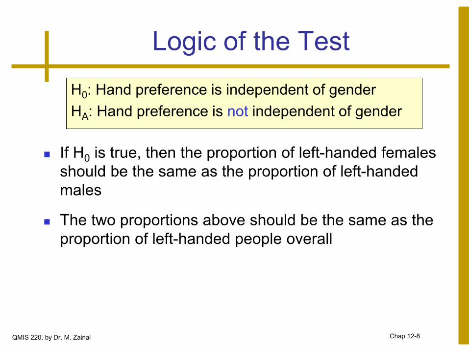
Logic of the Test

If H0 is true, then the proportion of left-handed females

should be the same as the proportion of left-handed

males

The two proportions above should be the same as the

proportion of left-handed people overall

H0: Hand preference is independent of gender

HA: Hand preference is not independent of gender


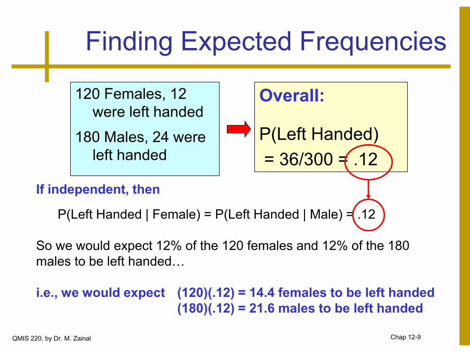
Finding Expected Frequencies

Overall:

P(Left Handed)

= 36/300 = .12

120 Females, 12

were left handed

180 Males, 24 were

left handed

If independent, then

P(Left Handed | Female) = P(Left Handed | Male) = .12

So we would expect 12% of the 120 females and 12% of the 180

males to be left handed…

i.e., we would expect (120)(.12) = 14.4 females to be left handed

(180)(.12) = 21.6 males to be left handed


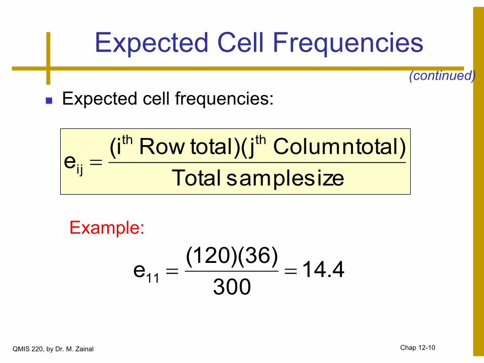
Expected Cell Frequencies

Expected cell frequencies:

(continued)

size sample Total

total) Column jtotal)(Row i(e

thth

ij

4.14300

)36)(120(e11

Example:


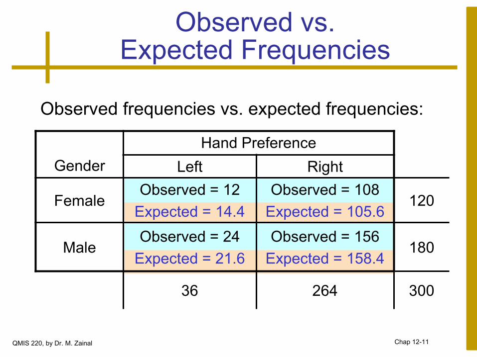
Observed vs. Expected Frequencies

Observed frequencies vs. expected frequencies:

Gender

Hand Preference

Left Right

Female Observed = 12

Expected = 14.4

Observed = 108

Expected = 105.6 120

Male Observed = 24

Expected = 21.6

Observed = 156


36 264 300


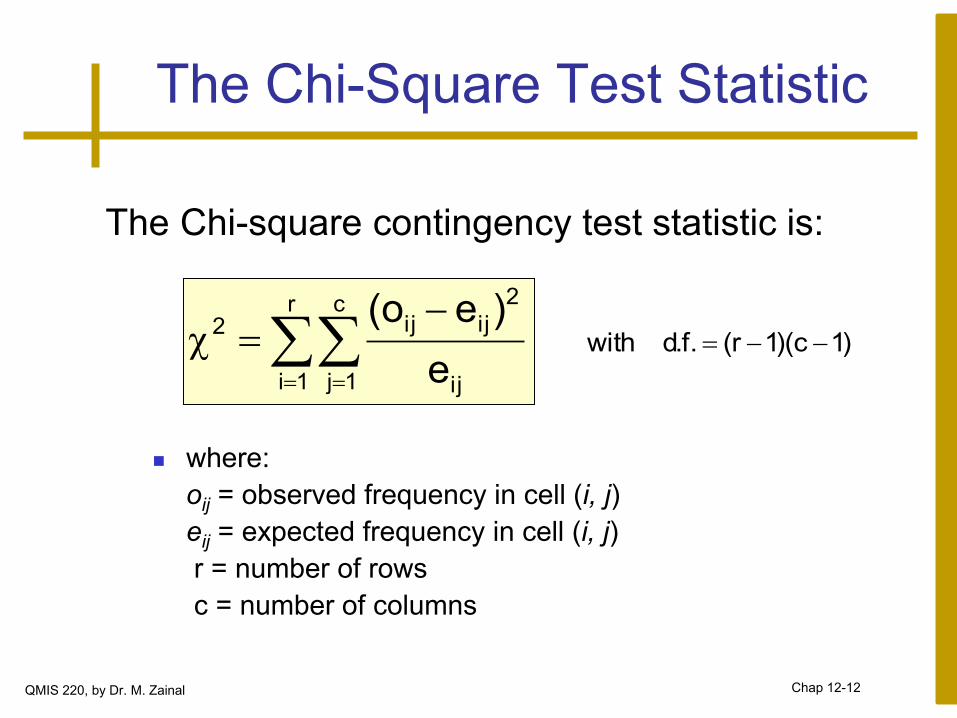
The Chi-Square Test Statistic

where:

oij = observed frequency in cell (i, j)

eij = expected frequency in cell (i, j)

r = number of rows

c = number of columns

r

1i

c

1j ij

2

ijij2

e

)eo(

The Chi-square contingency test statistic is:

)1c)(1r(.f.d with


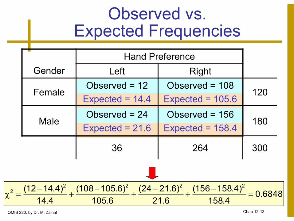
Observed vs. Expected Frequencies

Gender

Hand Preference

Left Right

Female Observed = 12

Expected = 14.4

Observed = 108


Male Observed = 24

Expected = 21.6

Observed = 156


36 264 300

6848.04.158

)4.158156(

6.21

)6.2124(

6.105

)6.105108(

4.14

)4.1412( 22222


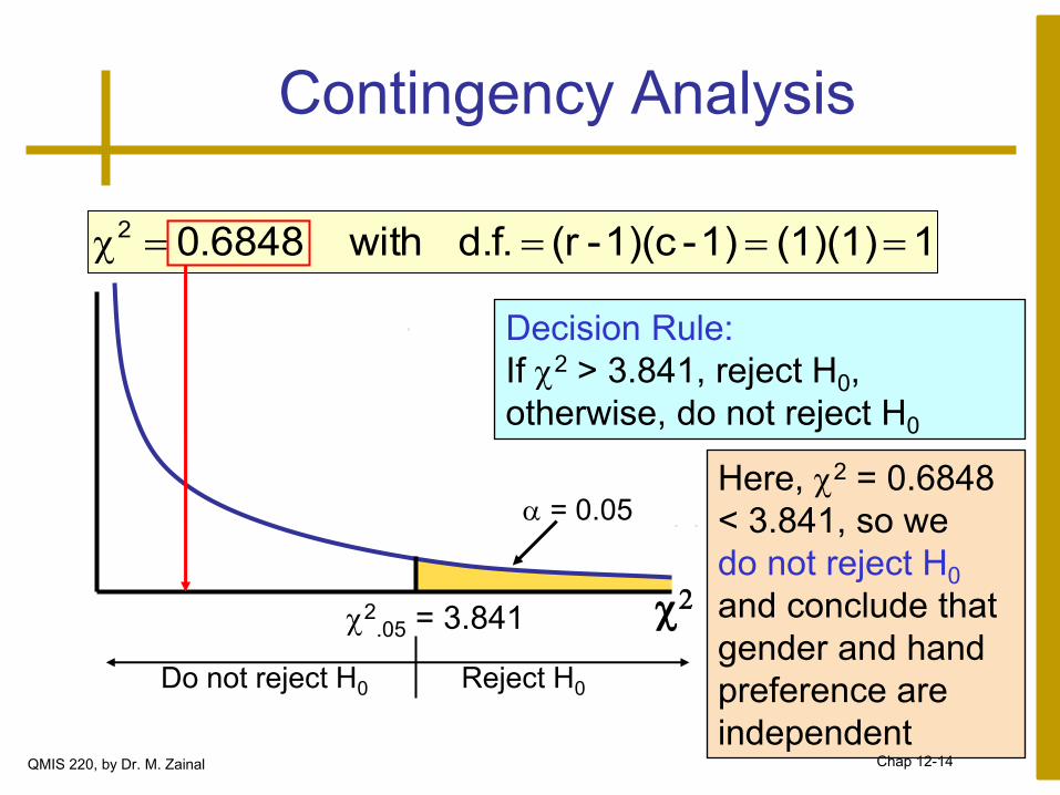
Contingency Analysis

2 2.05 = 3.841

Reject H0

= 0.05

Decision Rule:

If 2 > 3.841, reject H0,

otherwise, do not reject H0

1(1)(1)1)-1)(c-(r d.f. with6848.02

Do not reject H0

Here, 2 = 0.6848

< 3.841, so we

do not reject H0

and conclude that

gender and hand

preference are

independent QMIS 220, by Dr. M. Zainal Chap 12-14

Problem

QMIS 220, by Dr. M. Zainal

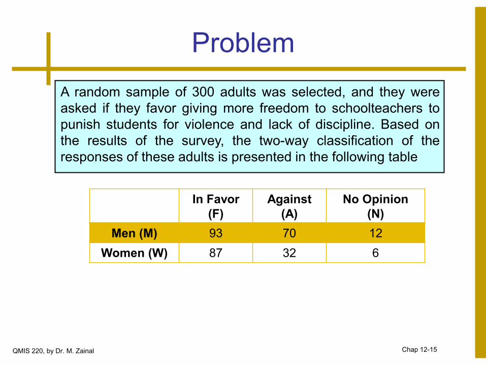
A random sample of 300 adults was selected, and they were

asked if they favor giving more freedom to schoolteachers to

punish students for violence and lack of discipline. Based on

the results of the survey, the two-way classification of the

responses of these adults is presented in the following table

In Favor

(F)

Against

(A)

No Opinion

(N)

Men (M) 93 70 12

Women (W) 87 32 6

Chap 12-15

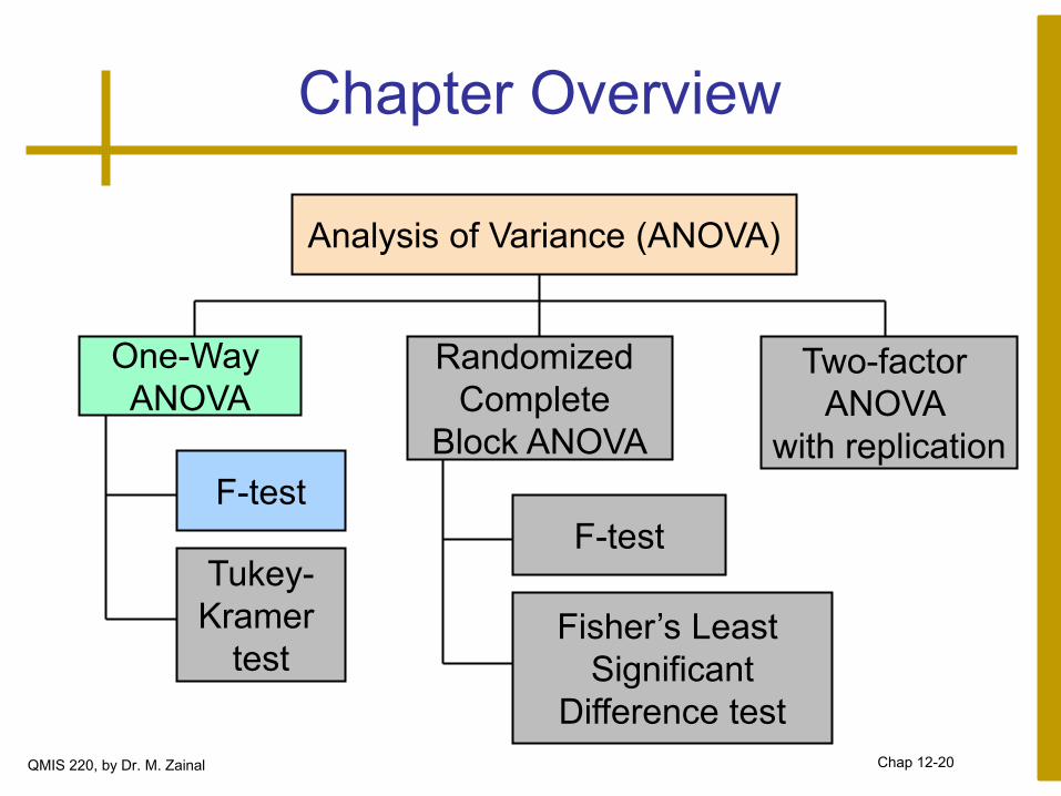
Chapter Overview

Analysis of Variance (ANOVA)

F-test

F-test Tukey-

Kramer

test Fisher’s Least

Significant

Difference test

One-Way

ANOVA

Randomized

Complete

Block ANOVA

Two-factor

ANOVA

with replication


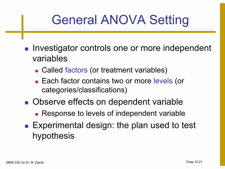
General ANOVA Setting

Investigator controls one or more independent

variables

Called factors (or treatment variables)

Each factor contains two or more levels (or

categories/classifications)

Observe effects on dependent variable

Response to levels of independent variable

Experimental design: the plan used to test

hypothesis


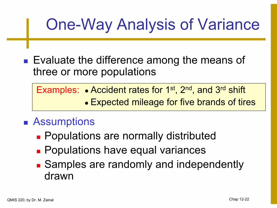
One-Way Analysis of Variance

Evaluate the difference among the means of three or more populations

Examples: ● Accident rates for 1st, 2nd, and 3rd shift

● Expected mileage for five brands of tires

Assumptions

Populations are normally distributed

Populations have equal variances

Samples are randomly and independently drawn


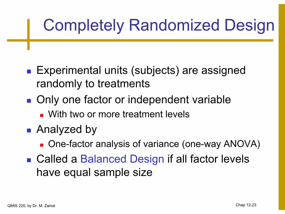
Completely Randomized Design

Experimental units (subjects) are assigned

randomly to treatments

Only one factor or independent variable

With two or more treatment levels

Analyzed by

One-factor analysis of variance (one-way ANOVA)

Called a Balanced Design if all factor levels

have equal sample size


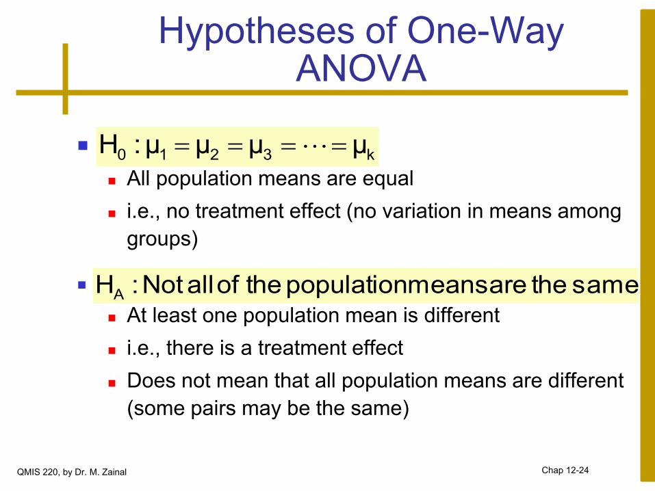
Hypotheses of One-Way ANOVA

All population means are equal

i.e., no treatment effect (no variation in means among

groups)

At least one population mean is different

i.e., there is a treatment effect

Does not mean that all population means are different

(some pairs may be the same)

k3210 μμμμ:H

same the are means population the of all Not:HA


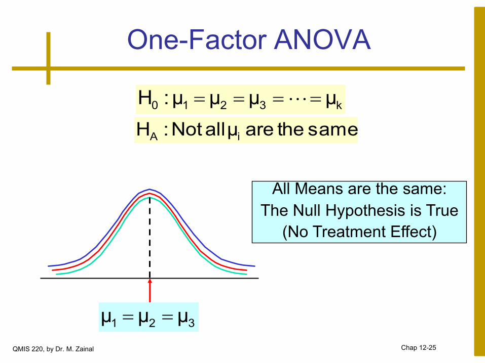
One-Factor ANOVA

All Means are the same:

The Null Hypothesis is True

(No Treatment Effect)

k3210 μμμμ:H

same the are μ all Not:H iA

321 μμμ


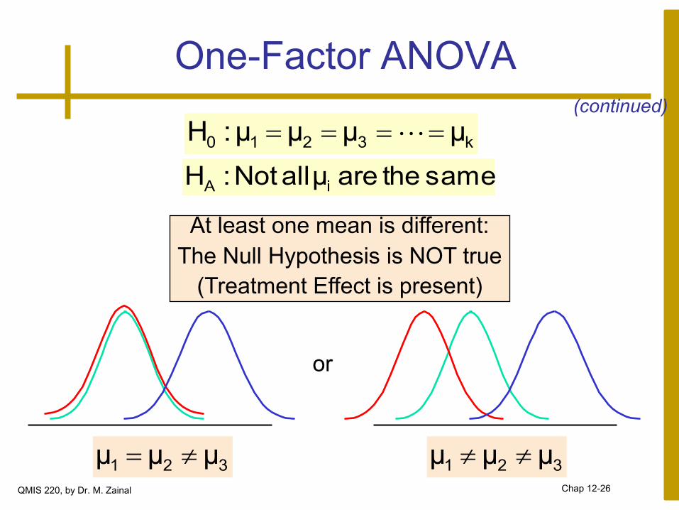
One-Factor ANOVA

At least one mean is different:

The Null Hypothesis is NOT true

(Treatment Effect is present)

k3210 μμμμ:H

same the are μ all Not:H iA

321 μμμ 321 μμμ

or

(continued)


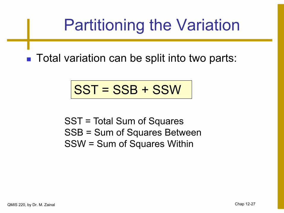
Partitioning the Variation

Total variation can be split into two parts:

SST = Total Sum of Squares

SSB = Sum of Squares Between

SSW = Sum of Squares Within

SST = SSB + SSW


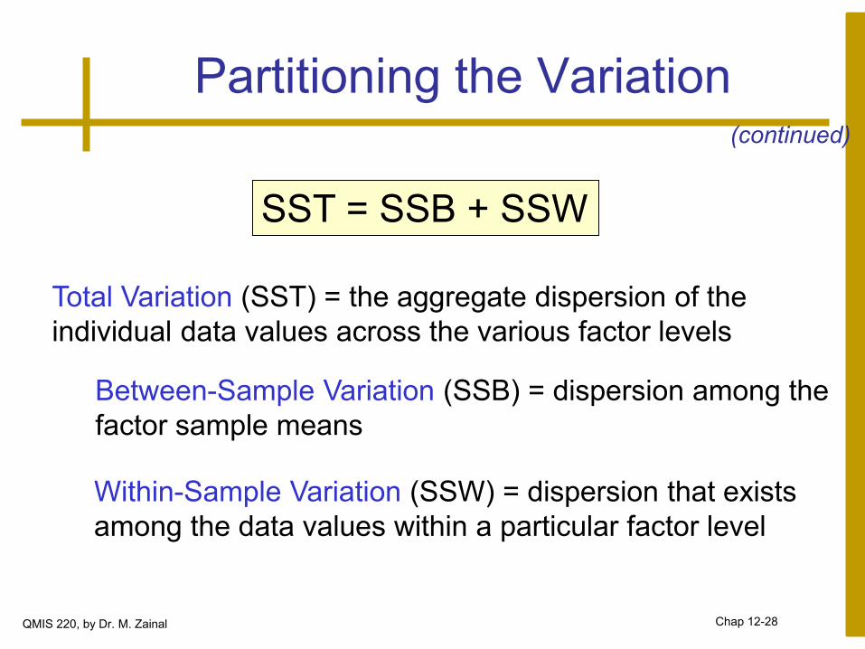
Partitioning the Variation

Total Variation (SST) = the aggregate dispersion of the

individual data values across the various factor levels

Within-Sample Variation (SSW) = dispersion that exists

among the data values within a particular factor level

Between-Sample Variation (SSB) = dispersion among the

factor sample means

SST = SSB + SSW

(continued)


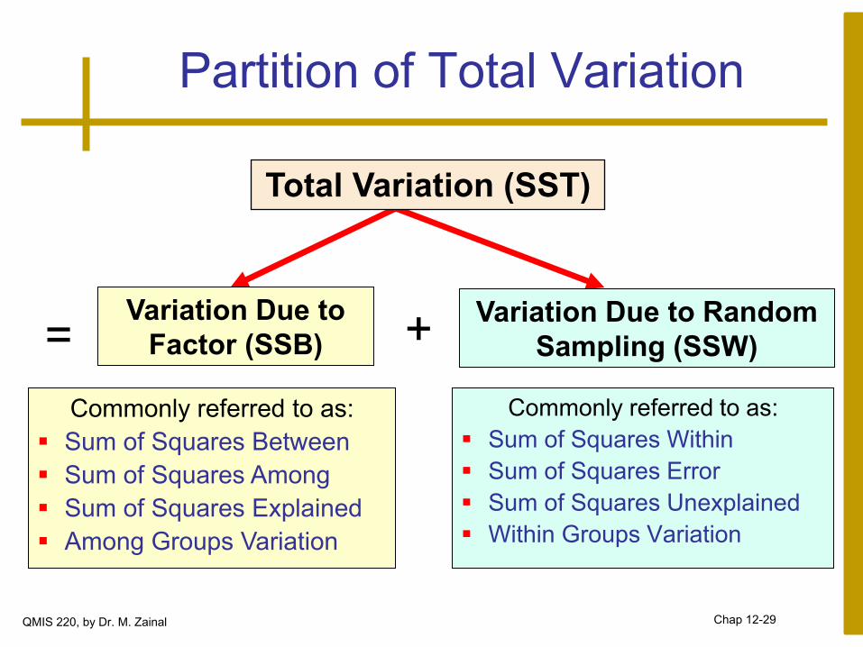
Partition of Total Variation

Variation Due to

Factor (SSB) Variation Due to Random

Sampling (SSW)

Total Variation (SST)

Commonly referred to as:

Sum of Squares Within

Sum of Squares Error

Sum of Squares Unexplained

Within Groups Variation

Commonly referred to as:

Sum of Squares Between

Sum of Squares Among

Sum of Squares Explained

Among Groups Variation

= +


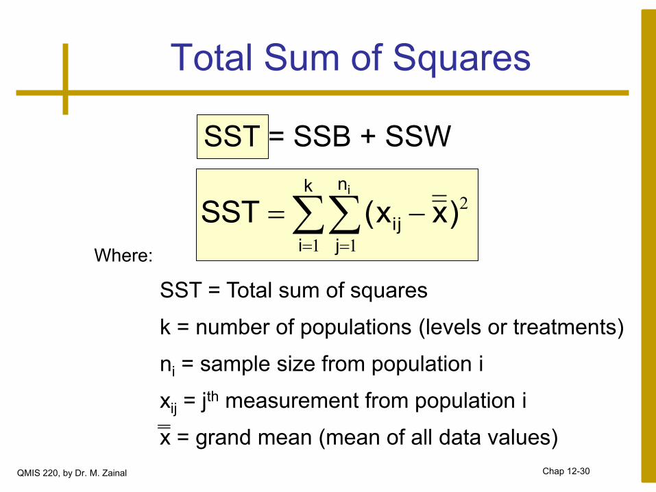
Total Sum of Squares

k

i

n

j

ij

i

)xx(SST1 1

2

Where:

SST = Total sum of squares

k = number of populations (levels or treatments)

ni = sample size from population i

xij = jth measurement from population i

x = grand mean (mean of all data values)

SST = SSB + SSW


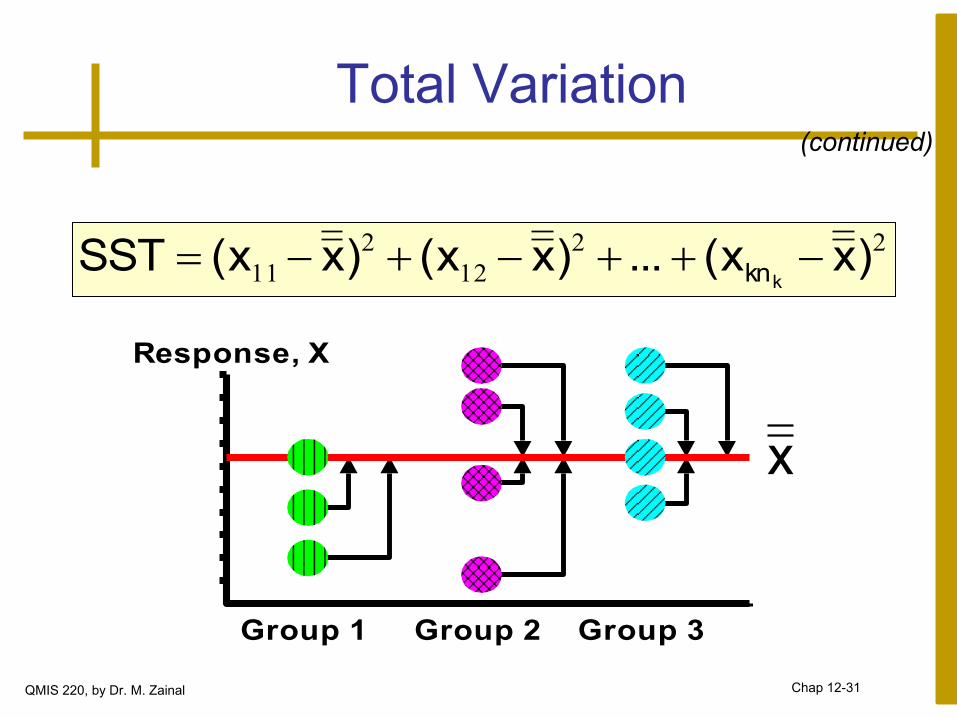
Total Variation (continued)

Group 1 Group 2 Group 3

Response, X

22

12

2

11 )xx(...)xx()xx(SSTkkn

x


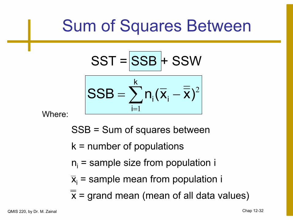
Sum of Squares Between

Where:

SSB = Sum of squares between

k = number of populations


xi = sample mean from population i

x = grand mean (mean of all data values)

2

1

)xx(nSSB i

k

i

i

SST = SSB + SSW


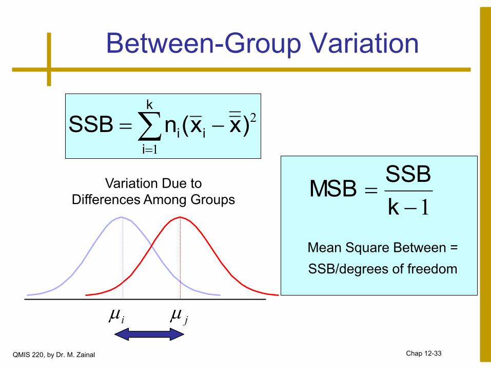
Between-Group Variation

Variation Due to

Differences Among Groups

i j

2

1

)xx(nSSB i

k

i

i

1

k

SSBMSB

Mean Square Between =

SSB/degrees of freedom


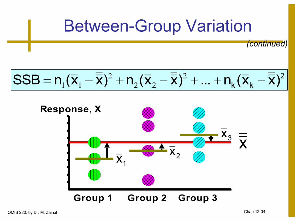
Between-Group Variation (continued)


Response, X

22

22

2

11 )xx(n...)xx(n)xx(nSSB kk

3x

1x 2xx


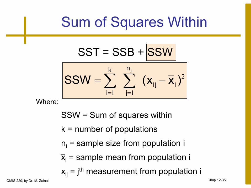
Sum of Squares Within

Where:

SSW = Sum of squares within



xi = sample mean from population i

xij = jth measurement from population i

2

11

)xx(SSW iij

n

j

k

i

j

SST = SSB + SSW


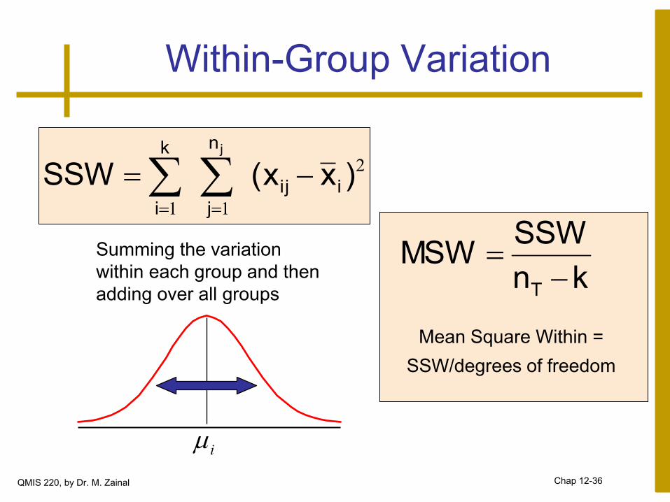
Within-Group Variation

Summing the variation

within each group and then

adding over all groups

i

kn

SSWMSW

T

Mean Square Within =

SSW/degrees of freedom

2

11

)xx(SSW iij

n

j

k

i

j


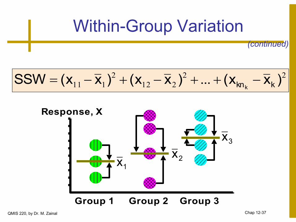
Within-Group Variation (continued)


Response, X

22

212

2

111 )xx(...)xx()xx(SSW kknk

3x

1x 2x


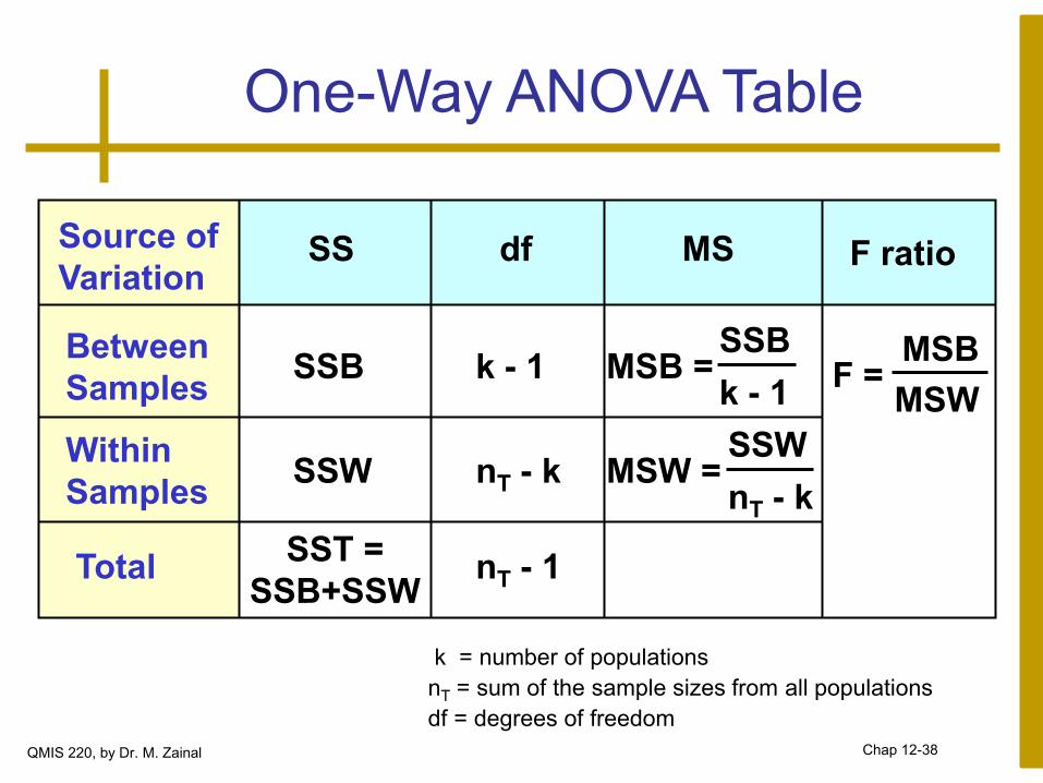
One-Way ANOVA Table

Source of

Variation df SS MS

Between

Samples SSB MSB =

Within

Samples nT - k SSW MSW =

Total nT - 1 SST =

SSB+SSW

k - 1 MSB

MSW

F ratio


nT = sum of the sample sizes from all populations

df = degrees of freedom

SSB

k - 1

SSW

nT - k

F =


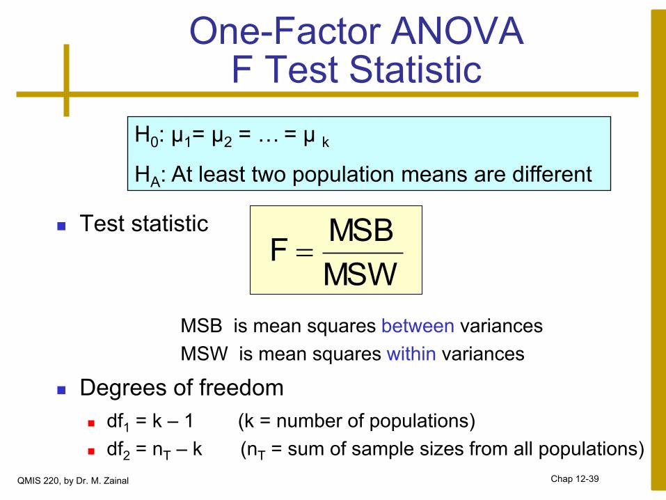
One-Factor ANOVA F Test Statistic

Test statistic

MSB is mean squares between variances

MSW is mean squares within variances

Degrees of freedom

df1 = k – 1 (k = number of populations)

df2 = nT – k (nT = sum of sample sizes from all populations)

MSW

MSBF

H0: μ1= μ2 = … = μ k

HA: At least two population means are different


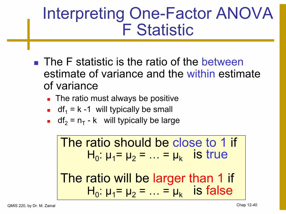
Interpreting One-Factor ANOVA F Statistic

The F statistic is the ratio of the between estimate of variance and the within estimate of variance The ratio must always be positive

df1 = k -1 will typically be small

df2 = nT - k will typically be large

The ratio should be close to 1 if H0: μ1= μ2 = … = μk is true The ratio will be larger than 1 if H0: μ1= μ2 = … = μk is false


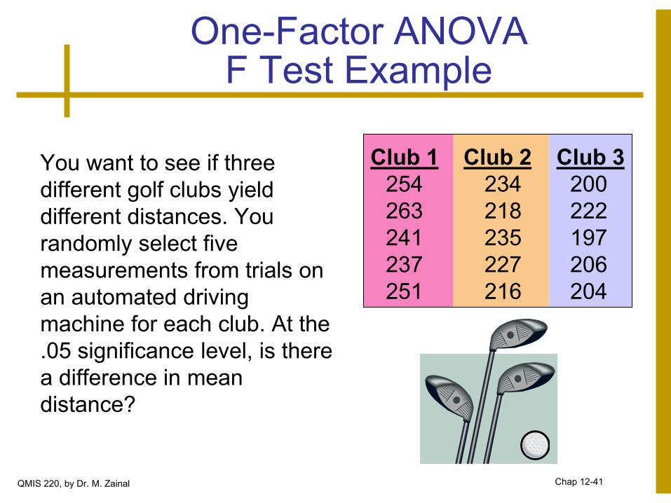
One-Factor ANOVA F Test Example

You want to see if three

different golf clubs yield

different distances. You

randomly select five

measurements from trials on

an automated driving

machine for each club. At the

.05 significance level, is there

a difference in mean

distance?

Club 1 Club 2 Club 3

254 234 200

263 218 222

241 235 197

237 227 206

251 216 204


• • • •

•

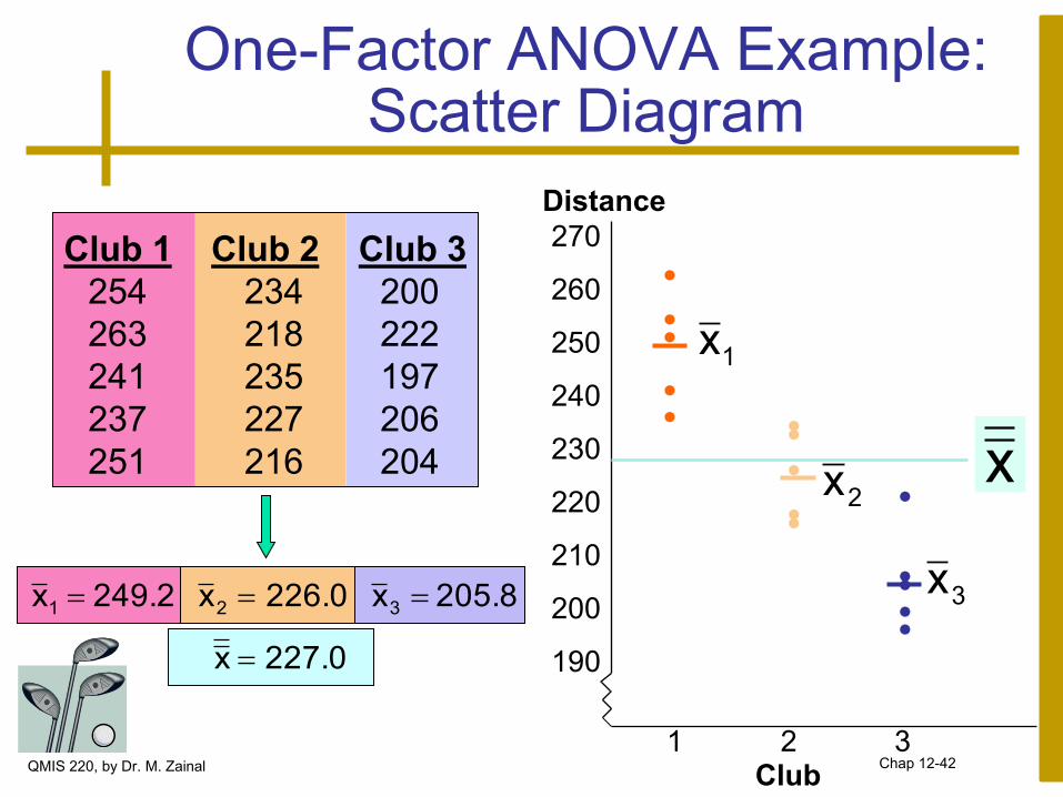
One-Factor ANOVA Example: Scatter Diagram

270

260

250

240

230

220

210

200

190

• •

• •

•

• •

•

• •

Distance

227.0 x

205.8 x 226.0x 249.2x 321


254 234 200

263 218 222

241 235 197

237 227 206

251 216 204

Club 1 2 3

3x

1x

2x x


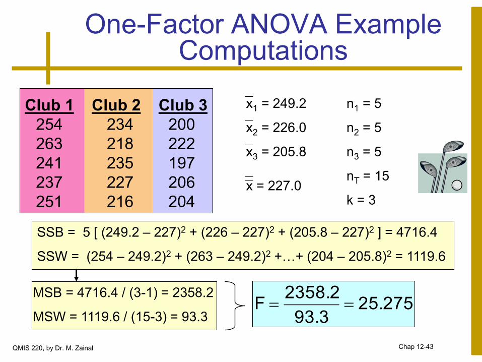
One-Factor ANOVA Example Computations


254 234 200

263 218 222

241 235 197

237 227 206

251 216 204

x1 = 249.2

x2 = 226.0

x3 = 205.8

x = 227.0

n1 = 5

n2 = 5

n3 = 5

nT = 15

k = 3

SSB = 5 [ (249.2 – 227)2 + (226 – 227)2 + (205.8 – 227)2 ] = 4716.4

SSW = (254 – 249.2)2 + (263 – 249.2)2 +…+ (204 – 205.8)2 = 1119.6

MSB = 4716.4 / (3-1) = 2358.2

MSW = 1119.6 / (15-3) = 93.3 25.275

93.3

2358.2F


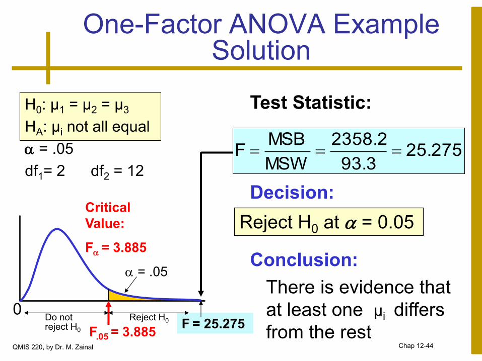
F = 25.275

One-Factor ANOVA Example Solution

H0: μ1 = μ2 = μ3

HA: μi not all equal

= .05

df1= 2 df2 = 12

Test Statistic:

Decision:

Conclusion:

Reject H0 at = 0.05

There is evidence that

at least one μi differs

from the rest

0

= .05

F.05 = 3.885

Reject H0 Do not reject H0

25.27593.3

2358.2

MSW

MSBF

Critical

Value:

F = 3.885


SUMMARY

Groups Count Sum Average Variance

Club 1 5 1246 249.2 108.2

Club 2 5 1130 226 77.5

Club 3 5 1029 205.8 94.2

ANOVA

Source of

Variation SS df MS F P-value F crit

Between

Groups 4716.4 2 2358.2 25.275 4.99E-05 3.885

Within

Groups 1119.6 12 93.3

Total 5836.0 14

ANOVA -- Single Factor: Excel Output

EXCEL: tools | data analysis | ANOVA: single factor


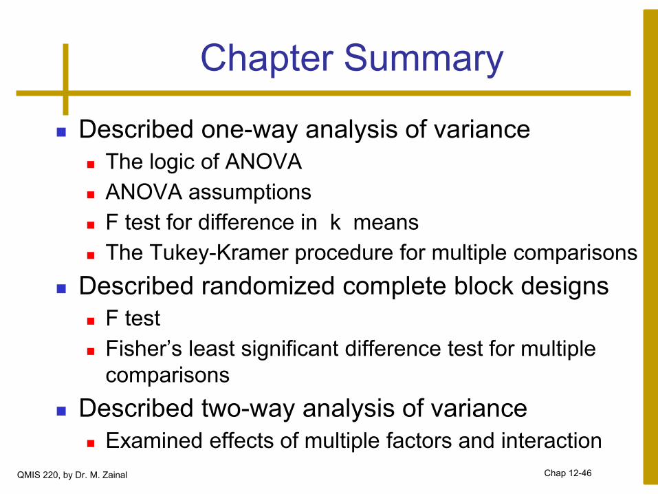
Chapter Summary

Described one-way analysis of variance

The logic of ANOVA

ANOVA assumptions

F test for difference in k means

The Tukey-Kramer procedure for multiple comparisons

Described randomized complete block designs

F test

Fisher’s least significant difference test for multiple

comparisons

Described two-way analysis of variance

Examined effects of multiple factors and interaction


Problems

QMIS 220, by Dr. M. Zainal

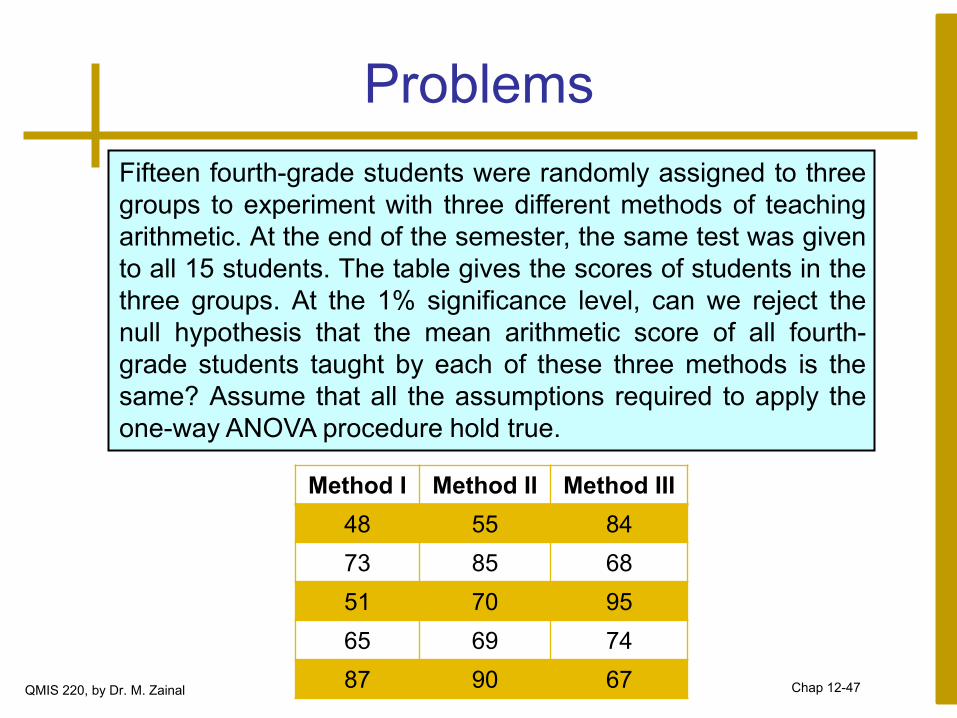
Fifteen fourth-grade students were randomly assigned to three

groups to experiment with three different methods of teaching

arithmetic. At the end of the semester, the same test was given

to all 15 students. The table gives the scores of students in the

three groups. At the 1% significance level, can we reject the

null hypothesis that the mean arithmetic score of all fourth-

grade students taught by each of these three methods is the

same? Assume that all the assumptions required to apply the

one-way ANOVA procedure hold true.

Method I Method II Method III

48 55 84

73 85 68

51 70 95

65 69 74

87 90 67 Chap 12-47

Chapter Summary

Described Chi square test of independency

Contingency tables

Described one-way analysis of variance

The logic of ANOVA

ANOVA assumptions

F test for difference in k means

Copyright

The materials of this presentation were mostly

taken from the PowerPoint files accompanied

Business Statistics: A Decision-Making Approach,

7e © 2008 Prentice-Hall, Inc.


Department of Quantitative Methods & Information Systems ... · Department of Quantitative Methods...

Documents

Transcript of Department of Quantitative Methods & Information Systems ... · Department of Quantitative Methods...