Department of Medical Physics and Engineering

“Realistic dynamic numerical phantom for the evaluation of acquisition methods in real- time Magnetic Resonance

Imaging of speech” by

P Joseph Martin

A dissertation submitted to the School of Medicine, King’s College London, in partial fulfilment of the degree of Master of Science in

Clinical Sciences (Medical Physics)

Local Supervisors: Marc Miquel and Redha Boubertakh

Academic Supervisor: Stephen Keevil

2 |

1

Contents

Acknowledgements ................................................................................................................................ 3

Declaration of Originality ..................................................................................................................... 4

Abstract ................................................................................................................................................... 5

List of Abbreviations ............................................................................................................................. 6

1 Introduction ......................................................................................................................................... 7

1.1 Human Speech: Functional morphology and pathologies .............................................................. 8

1.2 Medical Imaging in the clinical assessment of speech .................................................................... 9

1.3 Magnetic Resonance Imaging of speech ........................................................................................ 11

1.4 Computational Phantoms ............................................................................................................... 11

1.5 Advanced speech MRI techniques .................................................................................................. 12

1.5.1 Reducing acquisition times using accelerated parallel MRI ...................................................... 13

1.5.1.1 SENSE ....................................................................................................................................... 15

1.5.1.2 GRAPPA .................................................................................................................................... 16

1.5.2 Reducing acquisition times using Cartesian and non-Cartesian MRI ...................................... 17

2 Methodology ...................................................................................................................................... 20

2.1 Image Acquisition and Enhancement ............................................................................................ 23

2.2 Segmentation ................................................................................................................................... 24

2.2.1 Creation of a binary mask of the head and URT ........................................................................ 24

2.2.2 Outline areas containing organ of interest ........................................................................... 27

2.2.3 Create dynamic masks of organs of interest ............................................................................... 27

2.3 Mask optimisation ........................................................................................................................... 28

2.4 Continuous time model ................................................................................................................... 29

2.5 k-space phantom ............................................................................................................................. 31

3 Testing and Implementation ............................................................................................................ 31

3.1 Comparison of Cartesian and non-Cartesian Image Sampling Techniques ................................ 32

3.1.1 Aim of Investigation ..................................................................................................................... 32

3.1.2 Methodology ................................................................................................................................. 32

3.1.2.1 Creating k-space trajectories .................................................................................................... 32

2 |

2

3.1.2.2 Non-Cartesian k-space calculation .......................................................................................... 33

3.1.2.3 Investigations Considered ......................................................................................................... 35

3.1.3 Results........................................................................................................................................... 36

3.1.3.1 Spiral, Radial and Cartesian Imaging Comparison ................................................................ 36

3.1.3.2 Accelerated Radial Imaging ..................................................................................................... 37

3.1.5 Discussion..................................................................................................................................... 37

3.1.5.1 Spiral, radial and Cartesian image comparison ...................................................................... 37

3.1.5.2. Accelerated Radial Imaging .................................................................................................... 38

3.2 Comparison of accelerated parallel and conventional dynamic Cartesian MR imaging ............. 38

3.2.1 Aim of Investigation ..................................................................................................................... 38

3.2.2 Methodology ................................................................................................................................. 39

3.2.2.1 Dynamic Cartesian Images created using segmented through- time sampling ...................... 39

3.2.2.2 Creating undersampled multi-coil images ............................................................................... 40

3.2.2.3 GRAPPA and SENSE reconstructions .................................................................................... 42

3.2.2.4 Investigations considered .......................................................................................................... 43

3.2.3 Results........................................................................................................................................... 43

3.2.4 Discussion..................................................................................................................................... 44

3.3 Testing and implementation: Conclusion ...................................................................................... 48

4 Conclusion ........................................................................................................................................ 49

5 References .......................................................................................................................................... 50

2 |

3

Acknowledgements

I wish to thank the Barts Health MRI Physics group for hosting my MSc project.

In particular, I thank my local supervisors Marc Miquel and Redha Boubertakh,

who initiated and guided this project, as well as providing oversight, feedback

and most kindly their time throughout its duration. I also wish to Matthieu

Ruthven and Andreia Freitas who both made themselves available to answer

questions and provide assistance whenever asked.

I would like to thank my academic supervisor Stephen Keevil for his aid and

assistance.

I lastly wish to thank my family and friends, in particular my Mam without whom

I would have been unable to pursue a career in Science.

2 |

4

Declaration of Originality

I declare that, except where I have made clear and full reference to the

work of others, this project is my own work and has not previously been

submitted for assessment and I have not knowingly allowed it to be copied

by another student. I also understand that plagiarism is against the

regulations of King’s College London and that plagiarising another’s work

or knowingly allowing another student to plagiarise from my work, will

result in disciplinary proceedings.

“Realistic dynamic numerical phantom for the evaluation of acquisition methods in real- time Magnetic Resonance Imaging

of speech”

P Joseph Martin 23/03/2016

2 |

5

Abstract

Aim: Real time MRI (rtMRI) of human speech is an active field of research, with a particular clinical

focus on the assessment of speech disorders. In this work, a numerical phantom is developed to allow

acquisition and reconstructions schemes for rtMRI to be compared to a continuous time model of the

moving structures, which forms a dynamic computational phantom. The model is then tested using

different k-space sampling schemes (Cartesian, radial and spiral) and to simulate parallel imaging (PI)

reconstructions.

Methods: The computational phantom was developed using a prototyping software development

framework created in MATLAB (version 2016b, Mathworks, Natick, MA, USA). The whole

development process was split into two stages; (I) Phantom Development and (II) Testing and

Implementation (II).

Stage I. Phantom Development: Previously acquired 2D real-time MR images of a volunteer phonating

a standard speech sample were used. These images were then edge enhanced using the Canny1 method

and the relevant speech organs and structures segmented using a bespoke semi-automatic threshold tool.

These segmentations were used to create binary masks, which were processed using morphological

operators to make them more uniform resulting in 6 anatomical masks: ‘Mandible’, ‘Maxilla’,

‘Epiglottis’, ’Velum’, ’Tongue’ and ‘Head’. A continuous time motion model was then created by

linearly interpolating between two given masks in the time series. Finally, the 2D k-space phantom data

was derived as a time series using FFT and a non-uniform fast Fourier transform (NUFFT) for Cartesian

and non-Cartesian sampling trajectories respectively. The novel phantom has a simulated symmetrical

FOV of 30 cm, image matrix size of 256 x 256, k-space matrix size of 256 x 256, spatial resolution of

1.719 x 1.719 mm2, a temporal resolution of 30 fps and a single slice thicknesses of 10mm.

Stage II. Implementation and Testing: As a proof of concept two investigations were carried out. In the

first, the phantom was used to simulate Cartesian, radial and spiral trajectories and produce fully

sampled and accelerated images. In the second investigation, multi-coil undersampled dynamic images

were created and were used to test GRAPPA and SENSE reconstruction techniques by analysing a

parameter space including the temporal resolution, acceleration rate, number of coils and size of the

autocalibration signal region.

Results and Discussion:

A 2D speech MRI phantom has been developed that can be used to simulate k-space data sampled along

differing sampling trajectories. The two investigations found that the phantom could be used to produce

images in accordance with those produced clinically. This has been tested for radial, spiral and Cartesian

trajectories, and for undersampled Cartesian parallel imaging reconstructed. This phantom will allow

sampling trajectories to be optimised whilst ensuring they remain diagnostically useful.

Conclusion:

The first iteration of phantom development has been completed successfully. Future work would include

adding tissue contrast parameters (T1, T2) for each mask and using the phantom to test more advanced

dynamic imaging reconstruction techniques, such as across time kt-GRAPPA.2 Ultimately, a graphical

user interface would be produced to allow the end user to enter and alter imaging parameters to allow a

more interactive optimisation process.

This work will be presented at the International Society for Magnetic Resonance in

Medicine’s Annual Meeting in Paris on Monday 18th June 2018.

2 |

6

List of Abbreviations

2D – Two Dimensional

3D – Three Dimensional

ACS – Auto-Calibration Signal

ALS - Amyotrophic Lateral Sclerosis

BART - Berkeley Advanced Reconstruction Toolbox

bSSFP – balanced Steady State Free Procession

CRANE - Cleft Registry and Reporting Network

CT – Computer Tomography

DCF – Density Compensation Function

DICOM - Digital Imaging and Communications in Medicine

FE – Frequency Encoding

FFT – fast Fourier transform

fps – frames per second

FSTS – Fully-Sampled Temporally-Segmented

GRAPPA - GeneRalized Autocalibrating Partial Parallel Acquisition

LRT – Lower Respiratory Tract

MHRA - Medicines and Healthcare products Regulatory Agency

MR – Magnetic Resonance

MRI – Magnetic Resonance Imaging

NUFFT – Non-Uniform Fast Fourier Transform

PI – Parallel Imaging

PE – Phase Encoding

ROI – Region of Interest

RMSE – Root-Mean Square Error

SENSE – SENSitivity Encoding

SLT - Speech and Language Therapists

SNR – Signal to Noise Ratio

TSE – Turbo Spin Echo

URT – Upper Respiratory Tract

VPI- VeloPharyngeal Insufficiency

2 |

7

1 Introduction

In order to develop a useful numerical phantom for speech magnetic resonance imaging (MRI),

an understanding of both its clinical need and the advanced imaging techniques and sequences

required to perform it is neccesary. This is established in subsequent sections. Section 1.1-1.4

establishes the clinical importance of dynamic MRI of speech and how the creation of a

computational model would aid its development. Section 1.1 explains the anatomical mechanics

of human speech and pathologies that medical imaging can help diagnose, with a particular

focus on velopharyngeal insufficiency in patients born with a cleft palate. Section 1.2 discusses

the different imaging modalities available to speech and language therapists and other clinicians

to assess speech and its pathologies. Section 1.3 discusses in detail MRI of the speech organs

and the palate. Section 1.4 describes computational phantoms already utilised in MRI and how

a speech phantom would be implemented to improve clinical imaging.

The final section, 1.5, outlines two advanced MRI imaging techniques that are used in dynamic

speech MRI; parallel imaging (PI) (Section 1.5.1) and non-Cartesian acquisitions (Section

1.5.2); both commonly used to increase the temporal resolution of dynamic imaging. These will

form two test cases to assess the phantom in Section 3.

Figure 1.1 The upper and lower respiratory tracts. In human speech, when the diaphragm relaxes it pushes

air from the lower to upper respiratory tracts allowing the production of speech. This image was produced by

National Institutes of Health (NIH) and is in the public domain.

2 |

8

1.1 Human speech: functional morphology and pathologies

The production of human speech is a complex process using an interconnected system of

skeletal muscles working in co-ordination with the lower (LRT) and upper (URT) respiratory

tracts (Figure 1.1). A full discussion of the nuances of the mechanics can be found in Ball and

Rahilly 20003, but a simplistic understanding is adequate to develop an insight into the

requirements of a speech MRI phantom. The production of speech begins once the diaphragm

starts to relax after a person breathes in. The intercostal muscles contract as the diaphragm

relaxes causing the lungs to reduce in volume, and thus force air into first the bronchi and then

the trachea where it reaches the larynx, the beginning of the URT 4,5. The air is pushed through

a narrow gap in the larynx known as the vocal chords (or folds) (see Figure 1.2a). These vibrate

at a fundamental frequency (with higher harmonics), after which the air passes into the various

resonant cavities of the URT, whose dimensions are determined by the morphology and

positioning of the pharynx, velum (also known as the soft palate), jaw, tongue and lips. In the

phonation of non-nasal consonants, there is a further step, where the vocal tract is either partially

or fully occluded by a pair of articulators, e.g. the tongue and the hard palate (Figure 1B) or the

velum and the dorsal section of the tongue.4,5 Therefore, a healthy human can produce the full

range of sounds required for normal speech by controlling:

Figure 1.2 Functional Morphology of Speech. A) A sagittal view of the anatomy of the upper respiratory

tract, B) the anatomy of the palate. Adapted from Scott et al. 2014

A) B)

2 |

9

i) Respiration: the airflow through the vocal folds and URT by the diaphragm and

chest wall.6

ii) Phonation: the size, shape, tensions and separation of the vocal chords to control the

pitch of the sound. 6

iii) Resonance: the shape of the resonant cavities in the URT. 6

iv) Articulation: the effect of pairs of articulators (particularly for consonants). 6

There are however several maladies that can cause impaired speech, one of the most prevalent

being a cleft palate. According to the Cleft Registry and Reporting Network (CRANE), that has

been reporting on cleft patients in England, Wales and Northern Ireland since 2005, there are

an average 1,100 clefts diagnosed per year with 76% involving the palate.7 Patients with a cleft

palate will usually undergo surgery at 6-9 months, but 20% of patients have been found to

develop post-surgical velopharyngeal insufficiency (VPI).7 A common cause of VPI is the

inability of the velum to sufficiently occlude the entrance to the nasopharynx (velopharyngeal

closure), causing the patient to have difficulty in articulating certain consonants. These patients

are monitored and undergo speech and language therapy and may require further corrective

surgery between the ages of 3 and 10.8 Other maladies that may cause impaired speech are

diseases of the speech organs such as cancer, infections, polyps, nodules and cysts.5

Neurological conditions9 are also known to cause speech disorders; apraxia is often linked to

traumatic brain injury and stroke while dysarthria is the result of “disturbances in muscular

control over the speech mechanisms due to damage of the central or peripheral nervous

system”10 and is often linked to diseases such as multiple sclerosis, Huntingdon’s disease and

amyotrophic lateral sclerosis (ALS).11

To ascertain what treatments will be most effective for VPI, speech and language therapists

(SLTs) will initially perform a perception examination to assess resonance and articulation

during a speech sample. Many patients require further diagnostic evaluations, including medical

imaging. 12

1.2 Medical Imaging in the clinical assessment of speech

Imaging techniques are an essential tool for SLTs and surgeons when planning how best to

manage patients with VPI. The most commonly used techniques are nasendoscopy and

fluoroscopy. In nasendoscopy, a specialised fibre optic probe is passed through the nostril into

the nasal cavity from which the velopharynx can be viewed axially (Figure 1.3B).12,13 This is

more precise than fluoroscopy at discerning the degree of VPI and as it uses non-ionising

2 |

10

radiation it can be used multiple times, including during guided therapy sessions. Its

disadvantages are that its placement is somewhat invasive, which may directly affect the

patients quality of speech, and uncomfortable, which may make it difficult to use with a child

patient. Also, it gives only one two-dimensional (2D) view that provides no information of the

movement of the other articulators.12

In x-ray fluoroscopy (Figure 1.3A14), projection images of the patient performing speech tasks

are acquired with temporal resolution of 15-3015 frames per second (fps) and the height of

velopharyngeal closure can be determined, as can the movement of the tongue and pharyngeal

wall. However, as ionising radiation is used, the number of exposures has to be minimised

especially with paediatric patients, and as a consequence only a single lateral projection is

typically used. Furthermore, soft tissue contrast is poor although a barium colloid suspension

may be applied to the interior of the mouth to increase image contrast.16 Another disadvantage

is that as it is a projection, overlapping shadows may obscure organs of interest within the

image. The aforementioned drawbacks of both nasendoscopy and fluoroscopy have led

researchers to investigate other methods of assessment and MRI has been shown to be a viable

and potentially superior alternative.12

Figure 1.3. Medical Imaging of velopharyngeal insufficiency: A. is a sagittal videofluoroscopy view of the velum and

pharynx, with insufficiency assessed by measuring the distance between the two during attempted closure. Replicated

from Cuadros 2009. B shows nasoendoscopy examinations for three patients VPI is assessed as the area fraction of

the initially open areas that remains open during attempted closure. The top row shows 0% VPI, the second row 10%

and the third row 35%. Replicated from Ferreira 2015.

A. Videofluoroscopy B. Nasoendoscopy

2 |

11

1.3 Magnetic Resonance Imaging of speech

MRI offers excellent soft-tissue contrast allowing the tongue, velum and supporting muscles to

be imaged in any plane. Advances in dynamic MRI for gated cardiac imaging have led to the

development of fast sequences. In Cartesian imaging, Beer et al17 showed that they were able

to produced images of 5-6 fps using a Turbo Spin Echo (TSE) with 62.5% partial Fourier.

Advanced techniques such as accelerated parallel imaging reconstruction (20 fps with balanced

steady state free procession bSSFP)16 and non-Cartesian sampling trajectories (24 fps)18 have

also allowed increased temporal resolution, and are discussed in detail in Section 1.5.19 As no

ionisation radiation is used, studies can be performed multiple times and a microphone can be

used which allows a sound recording to be synchronised with the images. 4

Disadvantages include the necessity for the patient to lie in the supine position, which may

affect velar movement as reported in several studies. 17,20 However, Perry et al. (2012) found

only negligible effects on velar width, length or position due to gravity.21 Also, due to the long

time required to stay still in a noisy enclosed environment it is often hard to get children to co-

operate with such studies, although Tian et al. (2001) reported children of 5 years can be

cooperative if given adequate instructions. 22Additionally, the abundance of air to tissue

interfaces can cause susceptibility artefacts for all sequences, and banding artefacts for bSSFP

sequences. 19 Inevitably, image contrast will worsen, and the risk of other acquisition artefacts

is increased.23 This is problematic as the signal to noise ratio (SNR) will have to be sacrificed

to improve the temporal and/or spatial resolution(s). The use of non-Cartesian k-space sampling

trajectories can alleviate some of these problems and is discussed in Section 1.5.

As time on clinical MRI scanners is limited, computational phantoms may be used to pre-

optimise sequences before they are implemented and allow a fair comparison between

sequences by providing a ‘gold standard’ data set.

1.4 Computational Phantoms

The purpose of a computational (also known as numerical) MRI phantom, much the same as a

physical one, is to provide a standardised data set in which to test an imaging sequence.

Additionally, in a computational model the k-space sampling trajectory associated with a given

sequence may also be simulated. As mentioned above, in a busy clinical MRI unit, the time

available for physicists to optimise sequences on the scanners might be very limited, which has

necessitated the development of computational phantoms for other body parts. However, the

2 |

12

field suffers from a lack of standardised reference models, resulting inevitably in large body of

simulation methods hampering cross-validation between centres. 24

There are two principal types of computational phantom, analytical phantoms and voxel-based

phantoms. Analytical phantoms describe the simulated anatomy functionally. An early

successful example developed for CT is the Shepp-Logan brain phantom comprised of

overlapping ellipses of differing signal intensity. More specific MRI analytical head phantoms

were developed again using ellipses or geometric contouring.25-27 Voxel based phantoms rely

on the segmentation of a limited number of areas of interest pertinent to the study, resulting in

the aforementioned abundance of different models. As voxel-based phantoms mimic an actual

patient they are realistic, but their dimensions can be limited by the spatial and temporal

resolution of the original acquired image. Additionally for MRI, the k-space to image space

transformation used, the discrete Fourier transform, ignores k-space truncation errors, whereas

for an analytical phantom the continuous Fourier transform is well defined.24 However,

analytical phantoms do not usually incorporate the movement required for a speech phantom.

In an effort to overcome both of their hindrances, some have tried to create a hybrid phantom.

The MRXCAT uses voxel based, segmented, in-vivo data with either non-uniform rational b-

splines or a polygon mesh deformation model, which allows it to overcome the temporal and

spatial resolutions of the original segmented images.24 A similar methodology is applied to

simulate 2D MR images of velopharyngeal closure using binary masks instead of polygon

meshes in this work (Section 2.3).

The further development of MRI capable of assessing velopharyngeal closure and speech

disorders is reliant on the optimisation of imaging sequences to ensure that adequate spatial and

temporal resolutions can be achieved with sufficient signal while artefacts are minimised to

allow a correct diagnosis. A computational MRI speech phantom would allow for more

efficient sequence optimisation as well as create an environment to allow new sequences to be

explored and developed.

1.5 Advanced speech MRI techniques

As with all dynamic imaging, the key trade-off in speech imaging is having sufficient temporal

resolution to image the moving anatomy of interest whilst maintaining sufficient spatial

2 |

13

resolution, sufficient contrast and minimising artefacts enough to ensure these images are

diagnostically useful. Two increasingly prominent methodologies that aim to strike this balance

are non-Cartesian MRI and parallel MRI. Therefore, these will form two test cases (Section 3)

to assess the functionality of the computational speech phantom produced in this work (Section

2).

1.5.1 Reducing acquisition times using accelerated parallel MRI

A thorough description of parallel MR imaging can be found in Baert (2007)28. The underlying

principles utilised to be able to test the numerical speech phantom are herein explained. Parallel

imaging is so called because multiple receiver coils record the signal concurrently (i.e. in

parallel). This allows a means of reducing acquisition time by only filling a reduced proportion

of k-space, known as undersampling.29 The reduction in time is known as the undersampling or

acceleration rate (𝑅) and is defined as

𝑅 =𝑁𝑓

𝑁𝑠 [1]

where R is the ratio between the number of lines for a fully sampled k-space (𝑁𝑓) and the

number of lines ( 𝑁𝑠) actually sampled. In Cartesian imaging, undersampling only occurs in the

phase encoding direction as the frequency encoding direction is sampled from −𝑘𝑥,𝑚𝑎𝑥 to

𝑘𝑥,𝑚𝑎𝑥 concurrently, thus full sampling incurs no time penalty (non-Cartesian undersampling

and parallel imaging is also possible and briefly discussed in section 1.5.2). As the field of view

in the phase encoding direction (𝐹𝑂𝑉𝑃𝐸 ) is inversely proportional to the distance in k-space

between sampled lines (Δ𝑘𝑃𝐸), undersampling causes a reduction in 𝐹𝑂𝑉𝑃𝐸 proportional to 𝑅

and subsequently an aliased image (see Figure 1.4). However, using the data from the multiple

coils, along with some constraints and assumptions, allows one to in effect create simultaneous

equations (mathematically formulated as 2-dimensional matrix operations) that can be solved

to recreate the missing undersampled k-space data, and thus produce fully sampled, non-aliased

images (see Figure 1.4).29

2 |

14

The coils are often arranged in an array of known geometric proportions, and their sensitivity

to the target will be determined by their proximity to it. These parallel imaging coils are

typically smaller in size than larger single receiver coils and therefore ‘see’ (are sensitive to)

less noise and thus when combined to produce a single image (typically using the linear sum of

squares) they have higher SNR than the equivalent single coil image. This higher SNR can be

traded for decreased acquisition time and thus increased temporal resolution. 29 The biggest

penalty in using accelerated parallel imaging is a reduction in SNR, with the accelerated SNR

(𝑆𝑁𝑅𝑅) defined as

𝑆𝑁𝑅𝑅 =𝑆𝑁𝑅𝐹𝑆

𝑔. √𝑅 [2]

where g is the geometric or noise amplification factor, which is a measure of how easily the

‘simultaneous equations’ are independent and thus can be solved via a matrix inversion. g is

dependent on the coil geometry, k-space sampling trajectory, image plane being used as well as

the acceleration factor. The coil geometry is important as if two coils are too close together, and

Figure 1.4 SENSE parallel imaging and reconstruction with acceleration rate 2: Initially, images are

taken of the object to determine coil sensitivity maps. Then undersampled image of the object are taken

which are aliased and have ½ FOV of a fully sample image in the phase encoding direction. The coil

sensitivity maps allow the individual coil images to be unfolded using an inversion matrix, and the final

image is created by combing all the unfolded coil images using the sum of squares. Partially replicated

from Elster (2017).

SENSE Reconstruction

2 Acquisitions

1. Coil

Sensitivity Maps

2.

Undersampled k-space

Reconstruction

Unfold & Combine

Aliased single

coil images with FOV/2 in

PE direction

Images unfolded for

each coil using CSM and combined using

sum of squares

Phase Encoding Direction

2 |

15

their coil sensitivity maps too similar, small variations between the two, such as noise, are

amplified (hence its alternate name). The reconstruction will not be able to provide a

diagnostically useful image if the amplified noise becomes greater than the signal.28,30. Ideally

there would be g-factor of 1 across a map, but values of up to 1.2 are usually tolerable.28

The two most prominent parallel imaging reconstruction techniques, SENSE and GRAPPA are

explained in the subsequent sections.

1.5.1.1 SENSE

SENSE (SENSitivty Encoding) is performed in image space and uses the constraints of coil

sensitivity maps to allow fully sampled images to be recovered. It was developed by

Pruessmann et al31 and the imaging and reconstruction processes are summarised in Figure

1.4.32 Initially, coil sensitivity maps are calculated using fully-sampled images from each of the

coils. As mentioned above, acceleration causes aliasing, and an aliased image outside the field

of view is superimposed on the non-aliased image. The ingenious aspect of SENSE is that as

one knows the coil sensitivities for the superimposed images we can determine the proportion

of signal contributed from each and can thus reconstruct the original image for each coil using

an inversion matrix. These unaliased single coil images can then combined into a final image.

Scott et al16 used bSSFP parallel imaging and SENSE reconstruction to achieve diagnostic

speech MR images at 20 fps.

2 |

16

1.5.1.2 GRAPPA

GeneRalized Autocalibrating Partial Parallel Acquisition (GRAPPA), developed by Griswwold

et al33, is performed in k-space and uses the surrounding k-space data to estimate the non-

sampled portions of k-space. The process is summarised for a 2-coil and 𝑅 = 2 set up in Figure

1.5.32 GRAPPA fills in missing k-space data for each coil using a 2-dimensional kernel of

selectable dimensions for which it calculates weighting factors using a region of fully sampled

data, known as the autocalibration signal (ACS), from all coils. Then, the missing k-space data

for each coil is estimated using the surrounding data in the k-space for all coils. Again, an

inverse Fast Fourier Transform (FFT) produces images for each coil which are then combined.

The performance of GRAPPA reconstructions is comparable to SENSE for most imaging

techniques, however, it does not require coil sensitivity maps. This is especially useful in

heterogeneous areas such as the URT for which accurate coil sensitivity maps may be hard to

achieve.34

Figure 1.5 GRAPPA parallel imaging and reconstruction with acceleration rate: Undersampled images

of the object are taken for each coil, with the central region oversampled to allow it to be used to

calculate weighting factors for use in reconstruction. This missing k-space data for one coil is estimated

using weighting factors from all coils, and then individual coil images are produced used an inverse

FFT. The final image is created by combing all the unfolded coil images using the sum of squares.

Partially adapted from Elster (2017).

Acquisition

Combination

Sum of squares from individual Coil images

Oversampled Auto-callibration Signal (ACS) Region

k-space data estimation

Data driven interpolation using kernel

Individual Coil Images

Reconstituted using inverse FFT

GRAPPA Reconstruction

2 |

17

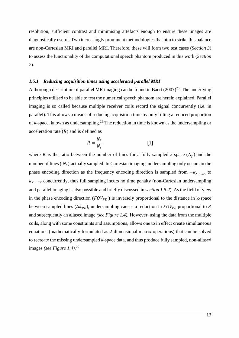
1.5.2 Reducing acquisition times using Cartesian and non-Cartesian MRI

In MRI, an imaging sequence is designed to fill k-space using one of several sampling

‘trajectories’, such as those shown in Figure 1.6. In the majority of modern imaging techniques,

this is done using a Cartesian grid, with orthogonal frequency (kFE) and phase-encoding (kPE)

directions. In terms of the sequence, a phase encoding gradient (𝐺𝑃𝐸) is applied that allows

sampling at a specific kPE value and then a frequency encoding gradient (𝐺𝐹𝐸) is applied during

signal acquisition to allow concurrent sampling of kx from -kx(max) to +kx(max). Then, another phase

encoding step (either during the same excitation using an echo sequence or after another

excitation) with a different gradient amplitude (𝐺𝑃𝐸′) is applied to sample at another specific

𝑘𝑃𝐸 value (Figure 1.6A). The number of lines sampled per excitation depends on the sequence

being used, but the process is repeated until k-space is filled to the extent required (some

imaging techniques that use only partially filled k-space are partial Fourier and parallel imaging;

see section 1.5.1 ).29 The path taken through k-space over time is known as the ‘trajectory’ and

is particularly important when using multi-echo techniques such as TSE, as relaxation occurs

between different lines of k-space, and therefore the time at which a particular line is sampled

will affect its contrast. Apart from single-shot techniques such as Echo Planar Imaging (EPI)

most Cartesian techniques require multiple excitations and therefore, it will take multiple TRs

to acquire a full image. In dynamic imaging, this leads to a lower temporal resolution and

Figure 1.6. k-space sampling points for different sampling trajectories: A shows a fully sampled k-space sampled using a

Cartesian sampling trajectory, represented stylistically in red. B shows k-space sample points from a spiral sampling trajectory,

which is shown in blue for one interleave and C shows radial sampling points with example spokes in green shown to represent

the radial trajectory.

A. Cartesian Fully-

Sampled k-space

trajectory B. Spiral k-space

sampling trajectory

C. Radial k-space

sampling trajectory

2 |

18

potentially to motion artefacts (the targeted anatomy is in different positions when different

parts of k-space are sampled). However, image processing is rather straightforward for

Cartesian sampling, simply requiring a two-dimensional FFT. 29

Unfortunately, acquisition times and temporal resolutions for Cartesian imaging can only be

reduced in speed to a certain point. To decrease the time of acquisition by half requires one to

quadruple the gradient slew rates (𝑑𝐺𝑃𝐸

𝑑𝑡) and double the maximum strengths (𝐺𝑃𝐸,𝑚𝑎𝑥), both of

which are limited by physiological constraints imposed by the MHRA to minimise the risk of

peripheral nerve stimulation.35,36 Therefore to improve speed whilst remaining within tolerable

limits, one needs to either use the gradients to cover k-space more efficiently or use less gradient

encoding.29 Non-Cartesian imaging sequences can utilise both of these techniques to achieve

reduced acquisition times.

Non-Cartesian MRI benefits from not utilising any phase encoding. In 2D applications,

following an excitation, two orthogonal gradients (Gx and Gy) are applied at the same time

during signal acquisition to take a sample line in k-space . In radial imaging, as in Figure 1.6C,

for a given excitation, Gx and Gy are constant and the angle (𝜙) of the radial line sampled through

k-space is determined trigonometrically by the relative amplitudes of the two gradients applied,

using

tan 𝜙 =𝐺𝑦

𝐺𝑥 [3]

and hence 𝜙 = 45𝑜when 𝐺𝑥 = 𝐺𝑦. Due to the rotation, the centre of k-space is fully sampled

but outer k-space locations are undersampled, and resultantly the centre of k-space must be

oversampled to achieve a fully sampled k-space. This requires more time (𝜋

2× 𝑡𝐶𝑎𝑟𝑡𝑒𝑠𝑖𝑎𝑛 ) than

for Cartesian sampling. This may seem counter intuitive when aiming to reduced acquisition

time and improve the temporal resolution of the speech imaging but the advantage is that when

undersampling k-space, the resultant artefacts are less apparent and coherent (radial streaking

and spiral ringing rather than superimposed copies of the image as in Cartesian undersampling4

and one can produce diagnostic images without the need for parallel image processing; see

section 1.5.1).4 However, if reconstruction is required to allow further undersampling, non-

Cartesian SENSE uses the conjugate gradient method to overcome the difficulty in locating

aliasing replicas, while non-Cartesian GRAPPA uses kernels only on small neighbourhoods.35

2 |

19

In spiral imaging, following the initial excitation, time varying 𝐺𝑥 and 𝐺𝑦 are applied to create

a path through k-space which follows an Archimedes Spiral. The k-space coordinates for an

equally spaced spiral can be derived as

𝑘𝑥(𝑡) =𝑁𝑠ℎ𝑜𝑡

2𝜋. 𝐿 𝜙(𝑡) sin 𝜙(𝑡) [4]

𝑘𝑦(𝑡) =𝑁𝑠ℎ𝑜𝑡

2𝜋. 𝐿 𝜙(𝑡) cos 𝜙(𝑡) [5]

where 𝑁𝑠ℎ𝑜𝑡 is the number of interleaved spirals and 𝐿 the field of view.29 The more interleaved

spirals, the less undersampled is k-space and artefacts are therefore reduced. Spiral acquisitions

are advantageous as they can cover a greater proportion of k-space in a single excitation when

compared to both Cartesian and radial acquisitions, and therefore can again potentially reduce

acquisition time. The highest reported temporal resolution for successful speech MRI was 22

fps using a spiral sampling trajectory.37

The greatest hindrance to both radial and spiral reconstructions is that the images cannot be

reconstructed using a simple FFT. There are other methods available, for example radial

imaging can use back projection (as was used by Lauterbur in 1973 to produce the first MR

images38) although this is inefficient. The most common methodology is a process called re-

gridding, where the data is resampled onto a Cartesian grid prior to reconstruction. This process

is not straightforward, and corrections must be made for the oversampled k-space centre (using

a density compensation function) and apodisation.29

2 |

20

2 Methodology

In this work, a dynamic 2D computational phantom was developed following a prototyping

software development framework, which can be seen in Figure 2.139 The computer code was

created in MATLAB version 2016b (MathWorks, Natick, MA, USA). The whole development

process is split into two overarching stages, Phantom Development (Section 2) and Testing and

Implementation (Section 3). Unless stated, all codes were written by the author.

The details of the methodology for developing the phantom, (stage I in Figure 2.1), can be

found below but are summarised here. Initially, time series images of a standard speech sample

were acquired at 100 𝑚𝑠 temporal resolution to attempt to adequately capture the motion of the

velum and tongue. Previous work at this centre suggests that frame rates of 10 fps or more

should be sufficient.40 These images were then edge enhanced (Section 2.1). The relevant

speech organs and structures were then segmented using a semi-automatic threshold method

(Section 2.2). These segmentations are then used to create binary masks, which are processed

using morphological operators to make them more uniform (Section 2.3). Then, a continuous

time motion model was created by interpolating between the masks (discussed in Section 2.4).

Finally, the k-space time series can be derived using a 2-D Fourier transform (Section 2.5). The

novel phantom produced has a simulated symmetrical FOV of 30 cm, image matrix size of 256

x 256, k-space matrix size of 256 x 256, spatial resolution of 1.719 x 1.719 mm2, a temporal

resolution of 30 fps and a single slice thicknesses of 10mm.

The flow of data and computational processes required to transform the dynamic DICOM

speech images into a computational phantom saved as a MATLAB data file can be viewed in

Figure 2.2. Five MATLAB scripts were created to process and manipulate the images, each of

which call functions both from the MATLAB standard library and image processing toolbox,

as well as novel functions and those made available online by the image processing community

which are referenced when used.

2 |

21

Figure 2.1 Software development framework for a novel Speech MRI Phantom. Stage 1. Phantom

Development shows the main processes involved in its creation, whilst the Stage. II Testing and

Implementation shows one use of the phantom to create images using Cartesian, radial and spiral sampling

trajectories.

2 |

22

Input: Individual

dynamic speech

organ ‘masks’

n ×

Single

“Image.mat” file

Image Volunteer

to produce a

series of DICOM

images at time t.

“DicomSeriesConverter.m”

Run this program to get the

data and header information

from each DICOM file, and

convert it to a single “.mat”

data file. See Appendix A

Individual

DICOM

files

“I_Run_PreProcessing.m”

runs the function [ImEE.mat]=

ImPreProcessing(Image.mat)

“II_MaskCreator.m”

“III_MaskManipulation.m”

“PhantomInterp.mat”

“IV_MaskInterpolation.m”

Optimised Masks

“PhantomMasks.mat”

Edge Enhanced

“ImEE.mat”

Phantom file which includes

Interpolated Masks and k-spaces

Function: “ImPreProcessing()”

Function: “INTERPMASK()”

Speech Organ

Segmented Masks

“Masks.mat”

Key:

DICOM Data

MATLAB Image File

MATLAB Phantom

Image and k-space file

MATLAB Function

Input and Output

Input:

“Image.mat”

file

Output:

“ImEE. mat”

file

Input: Individual

dynamic speech

organ ‘masks’

Function:

“bwmorph(‘options’)”

Function: “bwareaopen()”

Output:

Morphologically

Altered Masks

Input: Altered masks

Output: Masks with

small isolated areas

removed

Output:

Temporally

Interpolated

Speech Organ

Masks

Figure 2.2: Computational Framework and Data Flow to produce a computational phantom of speech from

dynamic speech DICOM files. The dark blue box represents the initial Speech MRI DICOM files and the

cyan box represents the resultant phantom saved as a MATLAB data file. The red boxes indicate bespoke

MATLAB scripts used to input image data and output further processed image data. The orange boxes

indicate important functions called in the scripts. The arrows indicate data flow, with colours explained in

the image key.

2 |

23

2.1 Image Acquisition and Enhancement

A previously acquired real-time MRI DICOM dataset (mid-sagittal images of the URT) of a

healthy adult volunteer performing speech samples was used as the base data for creating the

masks used in the phantom. Images were acquired at a temporal resolution of 10 fps and a

spatial resolution of 2.48 x 2.48 mm2. Imaging was performed using a 3 T Philips Achieva Tx

MRI scanner (Philips Medical Systems, Best, The Netherlands) at St. Bartholomew’s Hospital

for a project to investigate the required temporal resolution required to adequately capture

velopharyngeal closure in patients with normal speech.40 The speech samples the volunteer

were tasked with performing were designed to capture the full range of velocities and positions

of the tongue and velum during speech in English speakers.

After some initial attempts at segmentation, it was determined that edge enhancement of the

images would be beneficial to aid thresholding of the speech organs. Several methodologies

were tested including the Prewitt41 and an ‘Unsharp Masking’ method42 but it was determined

that the Canny method was the most effective in aiding segmentation (Section 2.2). The Canny

algorithm is a multi-stage process involving Gaussian filtering, image gradient detection and

multilevel thresholding.43 A MATLAB script was used to create and save a composite image of

the original time series and added edges (normalised and then multiplied by 0.2 of the maximum

intensity in the original image, this being found empirically to best aid segmentation). The

original image, the detected Canny edges and the sum image can be viewed in Figure 2.3.

= +

Figure 2.3 Canny Edge enhanced Speech MRI image of a volunteer: The edge enhanced image (right)

is created by summing the original image with the normalised (to 20% of the maximum of the original

image) detected Canny edges.

2 |

24

2.2 Segmentation

A semi-automatic process was used to create dynamic segmentations for five relevant speech

structures: the velum, tongue, epiglottis, mandible and maxilla. This was a 3-step process: the

first was to create binary masks of the whole head with the vocal and speech organs visible

(Section 2.2.1), the second was to select a region containing each organ of interest (Section

2.2.2) and the third was to automatically segment and create a mask for each organ of interest

at each time point (Section 2.2.3), resulting in binary masks of each of the speech organs of

interest for each dynamic frame in the original dynamic image set.

Section 2.2.1 Creation of a binary mask of the head and URT

Initially, a binary threshold was applied to the whole dynamic image series at a value set to a

100th of the maximum in the image which was found empirically to sufficiently maintain the

URT to allow segmentation. The resultant binary image, Figure 2.5, has ‘holes’ within it,

(defined in a binary image as ‘0s’ being completely surrounded by at ‘1s’ at any distance)

particularly in the cerebral spinal fluid around the brain, which are not physiologically relevant

for the speech phantom, as well as those forming part of the URT which are. 1 Hence, the next

step was to fill those holes that are not required to delineate the speech organs in the URT,

whilst maintaining those that are. This required some user input, and thus a new MATLAB

program was created. It produces an image prompt asking the user to select ‘holes’ in the head

outside the URT, as seen in Figure 2.5. This was performed on a single slice, but as the parts

of the head outside the URT remain relatively stationary throughout, the ‘hole’ positions can

be applied to the full dynamic data set.

Figure 2.4 Binary Mask of Canny Edge Enhanced 2D image of a volunteer performing a speech sample.

2 |

25

The next step was to fill in as much of the rest of the image as possible. The in-built MATLAB

function, imfill, a morphological process, is used to fill ‘all holes’ in the images on each

dynamic 2D image. This was selectively substituted into the user-selected ‘holes’ filled

images, with the ‘all holes’ filled image compromising everything from the bridge of the nose

upward as well as everything posteriorly to the trachea. This can be seen in the Figure 2.6.

This combination of user-directed and automatic filling attempts to fill all holes except the

upper respiratory tract. However, this process was not perfect and further morphological

processes are required to fill smaller holes outside the URT not filled previously.

+ =

Figure 2.6 Selective substitution of ROI to fill holes in a mask of speech to close all holes outside

upper respiratory tract. A. shows the selected region of interest in an image in which the user has

selected regions to fill. B shows the selected region in a mask with all holes automatically filled

and C shows the amalgamates images, created by selectively combining the two selected regions

in A and B.

+ =

User

Selected

Fill Points

Figure 2.5 User selected fill positions in an binary threshold mask of a 2D midline sagittal slice image

of human speech, performed by a volunteer.

2 |

26

A logical process (herein logical operators are defined as such in capital letters, eg. AND, OR)

aids the morphological operators in removing smaller holes in the mask. This process can be

seen in Figure 2.7. The amalgamated image produced previously is again shown in Figure

2.7A. In Figure 2.7B, all the ‘holes’ are again filled using MATLAB’s inbuilt ‘imfill’ function.

In Figure 2.7C shows the result of applying the logical operator B AND NOT A, leaving just

the holes that were filled. In Figure 2.7D, the MATLAB function ‘bwareaopen(‘Image’,

‘Threshold’)’ is applied to the ‘holes’ image to only leave the ‘holes’ with number of pixels

greater than a ‘Threshold’, defining ‘big holes’, which in this case was 23 to leave the

nasopharynx unfilled. Figure 2.7E shows the logical operations ‘holes’ AND NOT ‘bigholes’

to give the ‘small holes’. In the final image, Figure 2.7F, which was used for the segmentation,

is the logical operator A OR E, which will selectively fill only the ‘small holes’ defined in the

previous steps, and leaves the nasopharynx unfilled.

Figure 2.7 Logical process to remove non-physiologically relevant ’holes’ from the dynamic phantom masks.

A) is the phantom before this process. B) shows all ’holes’ filled in. C) shows the logical difference to show

all the holes that were filled. D) Only shows ’’holes” greater in size than 23 pixels, chosen to ensure the

nasopharynx ’hole’ is not filled as it is physiologically relevant to speech. E) is the holes minus those greater

than 23 pixels and F) is the resultant image with the ‘small holes’ filled but maintaining the nasopharynx.

nasopharynx

nasopharynx

2 |

27

Section 2.2.2 Outline areas containing organ of interest

User input was again utilised on a single slice to aid the latter segmentation. An area

sufficiently large to allow for full range of movement of an organ of interest (such as the

velum or tongue) was outlined directly onto the image using a freehand tool, ‘imfreehand’.

As the process was the same for each of the organs of interest, only the process for the velum

will be explained, but is applicable to all other structures.

Initially the user, in this case the author, was asked to outline an area to contain the velum, as

seen in Figure 2.8, and then, each of the other masks in turn. The user is advised to not be

concerned if there is some overlap between certain areas, e.g. ‘Mandible’ and ‘Tongue’ as

these will be accounted for using morphological and logical processes later (see section 2.3).

The aforementioned MATLAB function ‘imfreehand’ created handles for the image and for

the user selected velum segmentation area. These were then passed to the function

‘createMask’ which creates a binary mask where all the points within the selected region are

‘1’ and those outside the region are ‘0’.

Section 2.2.3 Create dynamic masks of organs of interest

Using a threshold binary mask of the area, the position and edge of each organ of interest at

each time-point t was recorded in separate image matrices. Overlapping segmentations may

occur at this point and are accounted for when the masks are optimised (Section 2.3). 2

Figure 2.8 User selected segmentation region: canny edge-enhanced mid sagittal slice of a volunteer’s head and neck,

with a user selected area in from which the velum will be segmented.

User Selected

Velum

Segmentation

Area

2 |

28

The program then ran automatically to segment the velum (and each of the other organs of

interest). Using the Hadamard product (a pixel by pixel multiplication), the user generated

region mask is multiplied by the sagittal mask of the head (a logical AND function would have

the same result) to give a binary mask of the velum to be used in segmentation.3

The segmentation itself used the MATLAB function ‘bwboundaries’. This function returns, for

each dynamic image, the boundaries of the all objects it can find in addition to binary images

of each of the segmentations automatically performed. The option 'noholes' tells it to not

segment any ‘holes’ within the object, which may occur particularly in the tongue due to a

magnetic susceptibility artefact in the original DICOM images. These will be filled when the

masks are optimised in the subsequent section.

2.3 Mask optimisation

In order to best visualise possible image artefacts, blurring and structure resolvability when

optimising an imaging sequence, it is ideal for the phantom to be as uniform as possible, while

still remaining anthropomorphic and retaining all physiologically important movement.

Therefore, a number of further automated binary morphological processes were performed.

These included ‘opening’ (morphological ‘erosion’ followed by ‘dilation’, see table

2.1),‘closing’ (‘dilation’ followed by ‘erosion’), the removal or isolated groups of pixels and

the filling of holes (principally in the tongue due to magnetic susceptibility artefact caused

signal drop out). These processes also smoothed rough protrusions from the edge of the masks.1

Then, a structured series of logical operators are applied to the masks (such as Mask A AND

(NOT Mask B)) to remove any overlap between them.1

= ×

Figure 2.9 Creating an image for the velum segmentation: The binary mask of the user-generated velum area is

multiplied on a pixel-by-pixel basis (Hadamard product) with the sagittal mask to create a binary image that will

be used to segment the velum.

Binary Mask of Velum Area that will be used for segmentation of the Velum

2 |

29

This process is automated. The MATLAB functions ‘imfill’ and ‘bwareaopen’ were again used.

Additionally, ‘bwmorph’ was used, which allows different morphological operators to be

utilised. Table 2.1 describes some of the principle operators used, some of which were used

multiple times.1

Morphological

Operator –

‘bwmorph()

property name’

Description Example

Erosion

‘thin’

This is the binary morphological process known as

erosion, which removes the outer most pixels from a

binary object using a 3 3 structural mask. Locations

where the structuring element fits inside the object

defines the outer locus points for the eroded object.

Dilation

‘thicken’

Dilation adds an extra pixel to the outermost layer again

using a 3 3 structural mask using the rule that where

the structuring element touches the object gives the new

outer locus points for the dilated object.

Diagonal

Fill –

‘diag’

This fills in the corners of objects when the background

is connected diagonally (known as 8 connectivity).

The final mask produced was of the head, and was created by logically subtracting all the other

masks from the binary image of the whole head created above (Figure 2.7F). This results in 6

anatomical masks: ‘Mandible’, ‘Maxilla’, ‘Epiglottis’, ‘Velum’, ’Tongue’ and ‘Head’. At this

stage, the phantom slices had been created from the original images, and the original dynamic

DICOM images were no longer used. The next stage was to interpolate through time between

the dynamic masks.

2.4 Continuous time model

Various methodologies were pursued to find the best method of interpolating between the

masks to create the continuous time model. Optical flow pixel velocities were calculated but

attempts to use these to create continuous deformation of the masks led to blurring and smearing

of the image.4 This smearing effect was again seen when attempting to perform non-rigid

Table 2.1 Description of binary morphological operators used to optimise a 2D dynamic masks of speech organ

for use in the creation of a dynamic speech MRI phantom.1

2 |

30

deformation using b-splines.5 To avoid smearing of the masks, image interpolation between the

masks was used6. This is calculated by utilising the Euclidian distance transform and

interpolating linearly between two given masks in the time series. The user can determine the

number of interpolated time steps between the masks, the number required dependent on the

imaging parameters being investigated, particularly echo time (TE) and repetition time (TR) in

terms of movement blur.

The interpolation was performed using the MATLAB function ‘interpmask’ which was

published in the MathWorks central file exchange community by Sven (2014).6 This method

uses a combination of the Euclidian distance transform and a linear model to interpolate the

movement of the edges of the mask between time points as required. It creates a matrix of the

Euclidian distance of each pixel to the edge of the mask then uses MATLAB’s inbuilt function

‘interp1’ to perform the actual interpolation.

As well as linear interpolation, cubic and spline-based methods are also available. These

methods were compared for each of the masks using the dice similarity coefficient (DSC) as a

comparative metric.7 Their accuracy is tested using the dynamic phantom of speech. Alternate

dynamic frames are removed from a dataset, with the interim frame interpolated from those

preceding and succeeding it. These are compared to the actual data, as well as each other using

a DSC. There was no statistically significant difference between the three methods, and

resultantly the linear method was used to minimise computational complexity.

Following the temporal linear interpolation, an image containing each of the different individual

organs masks (and the head) with varying contrasts was created, which form the dynamic 2D

images of the phantom.

Figure 2.10 Difference images for an interpolated time-point between two frames of the dynamic phantom.

Differences are shown in purple, and no differences are immediately apparent in this image

2 |

31

2.5 k-space phantom

The final step in the phantom development was to create for each dynamic image of the

phantom a corresponding k-space. The creation of the k-space is done using one of two

methodologies depending on whether it was to be used to simulate Cartesian or non-Cartesian

sampling trajectories, the discrete FFT or the non-uniform fast Fourier transform (NUFFT)

respectively.

The FFT was calculated using the MATLAB standard inbuilt 2-D discrete FFT function; ‘fft’.

However, to ease viewing of k-space transform it is useful, by convention, to have the zero

(origin) component at the centre of the image. This is achieved by using the inbuilt MATLAB

function ‘fftshift’ designed explicitly for this purpose before and after the Fourier transform is

performed. This k-space can be used to simulate all Cartesian k-space trajectories and therefore

it only needed to be calculated once.

The ‘NUFFT’ function used was created by Micheal Lustig, based on the work of Jeffrey

Fessler, and is part of the BART (Berkeley Advanced Imaging Toolbox) for Computational

Magnetic Resonance Imaging.12 It is necessary to use a NUFFT because the FFT only works if

both image speech and desired k-space are sampled uniformly on a Cartesian grid, which is not

the case for either spiral or radial sampling trajectories (see section 1.5.1). The NUFFT function

required as an input the non-Cartesian imaging trajectory and therefore this k-space must be

calculated for each trajectory simulated. This process is explained in detail in section 3.1. 8,9

3 Testing and Implementation

In Section 2, a dynamic MRI speech phantom was developed. The next step in the development

process was to test its usefulness for comparing different image sampling trajectories using

some scenarios used in MR speech imaging. In Section 1.5, the use of non-Cartesian, and

parallel imaging in speech MRI were discussed. In this section, as a proof of concept, two test

investigations were undertaken to determine if the phantom was a viable tool for comparing

imaging techniques. These investigations are:

i) A comparison of Cartesian and non-Cartesian image sampling trajectories (Section

3.1).

ii) A comparison of accelerated parallel and conventional dynamic Cartesian imaging

(Section 3.2).

2 |

32

In the subsequent sections, the aim of each investigation is stated, their methodology explained

and results reported. A discussion of each investigation follows, both of their results and, as

they collectively act as a proof of concept, the usefulness of the phantom as tool for simulating

k-space sampling trajectories. All images and k-spaces used have matrix dimensions of 256 ×

256 elements.

3.1 Comparison of Cartesian and non-Cartesian Image Sampling Techniques

3.1.1 Aim of Investigation

In essence, this investigation was a comparison of how k-space sampling trajectories effect the

image produced using the phantom, and if the differences are comparable to those found in

clinical speech MR images. Cartesian sampling is the standard k-space sampling scheme. It has

many advantages; it is easy to implement and allows the use of the FFT which is available on

all scanner platforms. Non-Cartesian sampling schemes have some advantages over Cartesian

ones, in particular speed and k-space coverage efficiency (see section 1.5), but reconstructions

are more complex and may have to be performed offline, diminishing its usefulness as a real-

time imaging technique. 10

3.1.2 Methodology

3.1.2.1 Creating k-space trajectories

This initial investigation compared fully sampled Cartesian k-space derived images for a single

time-point to simulated images created using both fully sampled and undersampled spiral and

radial imaging trajectories.

For the comparative Cartesian images, a fully sampled k-space for a given time-point, t, was

required. At present no tissue relaxation information is included in this phantom model and

therefore, the Cartesian k-space trajectory does not affect the image contrast. For non-Cartesian

sampling trajectories, the process for creating the images is more complex. As mentioned in

previous Sections (1.5.2 and 2.5), the phantom k-space cannot be determined before one knows

the sampling pattern, which must be specifically defined.

To create the sampling trajectories for spiral and radial imaging, two MATLAB functions were

written. The functions create a sampling pattern where the diameter ( 𝑛 ) of the sampling

trajectory (and the dimensions of the accompanying square k-space matrix) is defined, along

2 |

33

with the number of interleaves (𝑁𝐼𝑛𝑡𝑒𝑟𝑙𝑒𝑎𝑣𝑒𝑠) for spiral trajectories and the number of spokes

for radial trajectories (𝑁𝑆𝑝𝑜𝑘𝑒𝑠 ). If 𝑁𝐼𝑛𝑡𝑒𝑟𝑙𝑒𝑎𝑣𝑒𝑠 or 𝑁𝑆𝑝𝑜𝑘𝑒𝑠 are undefined, the function will

automatically calculate the sampling number to give a sampling that satisfies the Nyquist

criterion and is thus equivalent to a fully sampled Cartesian image. These are calculated using

equations

𝑁𝑆𝑝𝑜𝑘𝑒𝑠 = 𝜋𝑘𝑚𝑎𝑥𝐿 [5]

𝑁𝐼𝑛𝑡𝑒𝑟𝑙𝑒𝑎𝑣𝑒𝑠 = 𝜆 .2𝜋𝐿 [6]

for radial and spiral respectively, with L being the FOV, and 𝜆 a constant.10 Some example k-

space sampling trajectories can be seen in Figure 1.6.

3.1.2.2 Non-Cartesian k-space calculation

The overall process for creating the spiral and radial trajectories can be viewed in Figure 3.1

for a spiral example. This process used functions from the ‘MRiLAB’ toolbox created by Fang

Liu at the University of Wisconsin-Madison.11 NUFFT was again performed using the

‘NUFFT’ function created by Micheal Lustig, based on the work of Jeffrey Fessler, and is part

of theBART.12 This function requires three inputs:

i) the phantom image for a given time point (created in Section 2),

ii) the k-space sampling trajectories (created in Section 3.1.2.1),

iii) and the density compensation function (DCF).

2 |

34

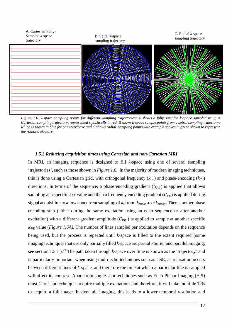
The DCF is required to compensate for the intrinsic oversampling of the centre of k-space when

using spiral and radial sampling trajectories.13 It is calculated using a function from the

‘MRiLAB’ toolbox which uses a Voronoi diagram calculated using an inbuilt MATLAB

function. A Voronoi diagram creates cells around each data-point such that all are bounded by

a locus of the equidistant position between the point and the next nearest point in a given

direction (see Figure 3.2). This leads to no overlapping cells, and the area of a given cell in

proportional to the inverse of the local density of points.

The ‘NUFFT’ process creates the non-uniformly sampled k-space, and then a subsequent

process is used to re-grid it. This is a data-driven implementation in which a kernel is used to

spread data from each k-space sample point to adjacent grid points. This is more SNR efficient

than grid-driven interpolation as it uses all the data, however, it requires the data to be density

compensated before gridding. In certain cases, Gaussian noise was added to the re-gridded k-

Figure 3.1 Simulation process for spiral k-space sampling trajectories. A. is a phantom image from a given

time point, B. shows the sampling trajectories in k-space and C. shows the density compensation function

(DCF) derived by created a Voronoi diagram. D. shows the k-space created when inputting A-C into a

NUFFT function and then re-gridding onto a Cartesian grid. E shows the simulated image recovered using

an inverse FFT.

2 |

35

space to simulate noise produced in signal detection. The re-gridded k-space was then used to

create the final simulated image using an inverse FFT.

3.1.2.3 Investigations Considered

This methodology was used to perform two basic investigations:

i) A qualitative and quantitative comparison of fully sampled spiral, radial and

Cartesian images.

ii) A qualitative and quantitative review of undersampled radial images created with

acceleration factors (𝑅) of 1, 2, 4, 8 and 16.

The quantitative metric used to compare the images was the root mean squared error (RMSE),

calculated for two images using the following equation:

𝑅𝑀𝑆𝐸 = √𝐼

𝑛. 𝑚∑ ∑[𝐼𝑚2(𝑥, 𝑦) − 𝐼𝑚1(𝑥, 𝑦)]2

𝑛−1

𝑥=0

𝑚−1

𝑥=0

[7]

This is an objective fidelity criterion1 and is useful for comparison as it is not dependent on the

image rater. The qualitative metric used is a discussion of how well the speech organs can be

distinguished in the images. This is a subjective fidelity criterion often used in speech MRI14,15

and was performed by the author.

Figure 3.2 Voronoi diagram of spiral k-space sampling points. The cells for each point are bound by the

locus of the point of equidistance between it and its nearest neighbour in a given direction. As a result,

none of the cells overlap and a given cell area is inversely proportional to the local density of points.

2 |

36

3.1.3 Results

3.1.3.1 Spiral, Radial and Cartesian Imaging Comparison

Example reconstructed images for Cartesian, spiral and radial trajectories can be viewed in

figure 3.3, along with the RMSE calculated in comparison to the Cartesian sampled image from

the phantom. The top row has images with no added noise, and the bottom row shows images

with Gaussian noise added prior to NUFFT being performed. The noise had a maximum

intensity of 5% of the maximum intensity of the original image.

Figure 3.3: MRI speech phantom reconstructions using spiral k-space sampling trajectories: The left

hand depicts a Cartesian image of the phantom at a given time-point, the centre image has a

reconstruction of the same image with a radial trajectory and the right hand uses a spiral

reconstruction. The top row contains images produced with no added Gaussian noise while the bottom

row has images created with 5% Gaussian noise added to the original phantom images prior to the

NUFFT and non-Cartesian sampling.

2 |

37

3.1.3.2 Accelerated Radial Imaging

The simulated effect of acceleration can be seen in Figure 3.4. The root mean squared error

for each of the simulated images compared to the original phantom (and compared to 𝑅 = 1

were applicable) is displayed with each corresponding image.

3.1.5 Discussion

3.1.5.1 Spiral, radial and Cartesian image comparison

In terms of the subjective criteria, both the spiral and radial sampling trajectories allowed the

individual speech organs to be viewed with and without 5% Gaussian noise added, which is the

basic functional task required of these images in clinical speech MRI. The radial images showed

the intrinsic ring aliasing artefact associated to it, as well as Gibbs artefacts near the edges of

each of the speech organs, the latter of which has been reported in clinical radial imaging and

is caused by the re-gridding process.16 In the spiral images, a very streaked background noise

was apparent across both of the images and this is again reported in clinical imaging as an effect

of re-gridding16, and in this case, is an effect of multiple uncorrelated aliased images. Unlike

in Cartesian imaging where the correlated aliased repetitions can obscure the anatomy of

interest, these aliasing artefacts did not affect the diagnostic efficacy of the image.

In quantitative terms, the RMSE was greater for radial than spiral (22.1% to 18.6%) without

added noise. However, the noise had little effect on the radial images RMSE, 22.6%

corresponding to a 2.26% increase, whereas it led to a 32.80 % greater RMSE for the spiral

trajectory (24.7%). However, in terms of the task of identifying the speech organs, the noise

Figure 3.4 Simulated Images of a speech MRI phantom produced using radial k-space sampling trajectories: The

extreme left-hand image shows the initial “true” image of the phantom and the images to its right are generated

using radial sampling trajectories with increasing under-sampling factors (indicated above each image). The

normalised root mean square (RMS) error of pixel intensities.

(RMS Error compared to R=1): (2.63%) (5.94%) (11.38%) (20.15%)

2 |

38

and artefacts would not prevent a clinician from diagnosis, and thus these images would be

likely just as useful as the original Cartesian images.

3.1.5.2. Accelerated Radial Imaging

In figure 3.4, as the acceleration rate increases, the abundance and prevalence of radial streaking

artefacts also increases; this is in accordance with previously reported results.17,18 There also

was a reduction in contrast between the speech organs with increasing acceleration rate, as

should be expected when the centre of k-space becomes less sampled. Additionally, there was

an increase in background noise due to the un-correlated aliased repetitions of the image, again

as reported in the literature.16,18 However, even with an acceleration rate of 8, the position of

each of the speech organs of interest could still be determined, although at an acceleration rate

of 16 the combination of streaking artefacts, increased noise and reduced contrast resulted in a

non-diagnostic image. The RMSE was in accordance with these findings, with radial image

RMSE with no acceleration being 22.1%, the last diagnostically useful image (𝑅 = 8) being

28.2% (RMSE of 11.38% compared to 𝑅 = 1) whilst the non-diagnostic image had a much

increased RMSE value of 36.3% (20.15% compared to 𝑅 = 1).

3.2 Comparison of accelerated parallel and conventional dynamic Cartesian MR imaging

3.2.1 Aim of Investigation

As highlighted in Section 1.5.1, accelerated parallel imaging has been utilised in speech imaging

to provide temporal resolutions greater than 20 fps.15 In this work, dynamic images of varying

temporal resolutions were reconstructed using the GRAPPA and SENSE reconstruction

techniques from simulated undersampled dynamic Cartesian temporally-segmented images.

These were then compared to each other and fully-sampled temporally segmented (FSTS)

dynamic images.

2 |

39

3.2.2 Methodology

3.2.2.1 Dynamic Cartesian Images created using segmented through- time sampling

The phantom k-space was sampled in a way designed to created dynamic FSTS Cartesian

images with a specified temporal resolution. This process is shown stylistically in Figures 3.5

and 3.6. Multiple k-space lines, known as segments, are taken from different subsequent time-

points until the entire k-space is filled. The k-space is filled from +𝑘𝑥,𝑚𝑎𝑥 to −𝑘𝑥,𝑚𝑎𝑥 , with the

number of segments (and phantom time-points used) dependent on the desired temporal

resolution. This methodology leads to temporal blurring artefacts.

Figure 3.5 Image with temporal resolution of 133 ms produced using segmented through time sampling

of the k-space of a speech MRI phantom with temporal resolution of 33 ms. Temporal blurring is apparent

in the created image.

Phan

tom

Imag

es

Phanto

m

k-sp

aces

Tem

pora

lly-

segm

ente

d

k-sp

ace

Tem

pora

lly-

segm

ente

d

Imag

e

2 |

40

These TSFS dynamic k-spaces were used as the basis for creating undersampled dynamic

images that are discussed in the next section.

3.2.2.2 Creating undersampled multi-coil images

The creation of undersampled coil images was based around two processes; the initial

calculation of multi-coil images from the phantom and then the subsequent simulation of

undersampled images for each coil. The first process is represented in Figure 3.7 for a simulated

8-element array coil. A set of MATLAB programs and functions were created to achieve this

(available in the supplementary material). A function creates complex coil sensitivity maps

based on 2D Gaussian distributions when provided with the desired number of coils (which are

assumed to be equidistant from the centre of the field of view), the angular location of the first

coil and the dimensions of the phantom image in use. The Hadamard product of the complex

coil sensitivity maps, the temporally-segmented dynamic series image (at a given time point)

and Gaussian noise images creates the desired individual coil images.

Figure 3.6: k-space derived for two temporal resolutions from a dynamic k-space phantom sampled using through

time to create an image with simulated temporal resolution using temporal segmentation of different time points

from a dynamic k-space phantom of temporal resolution of 33 ms: The left hand image shows the k-space sampling

pattern at 7.5 fps created in 4 segments, each taken from 4 different time points in the phantom. The right-hand

image shows the k-space sampling for a dynamic image at 3.25 fps.

2 |

41

Another function creates the undersampled k-spaces for each coil for each frame of the

simulated dynamic series. The process for a single time-point and single coil can be seen in

figure 3.8. This function allows one to select the acceleration rate (𝑅) and also the number of

fully sampled calibration lines, required for GRAPPA reconstruction, but not for SENSE. The

Figure 3.7: Creating individual coil images for a simulated 8-element array coil: The Hadamard product of

simulates fully-sampled temporally segmented (FSTS) phantom image(A), the complex coil sensitivity(B) and

complex Gaussian noise(C) produce simulates individual coil images(D).

Figure 3.8: Producing Undersampled Images for each coil. An FFT (B) of the individual coil images (A) is

multiplied on a element by element basis by the desired undersampling pattern (C). An inverse FFT of this

product is then performed to produce the undersampled coil image (D).

2 |

42

difference in aliasing pattern with and without a fully sampled auto-calibration signal region at

the centre of k-space can be seen in figure 3.9.

The function takes in the undersampled image series for each coil and converts it to k-space

time series using a FFT. It also creates a binary undersampling pattern for a given input value

of 𝑅. To save computing time this 2D pattern is replicated in a third (in this case temporal)

dimension so that is has the same dimensions as the FSTS dynamic image series. Then for each

coil one can use a three-dimensional Hadamard product of the dynamic fully sampled

temporally-segmented k-space and the 3D replicated undersampling pattern to produce the

undersampled k-space. The undersampled single coil images can be retrieved using an inverse

FFT.

3.2.2.3 GRAPPA and SENSE reconstructions

The GRAPPA and SENSE reconstructions were performed using functions from the BART.12

The GRAPPA function requires the undersampled k-space for each of the coils, the acceleration

factor and a coded undersampling pattern, such that ‘1’ is sampled data, ‘0’ undersampled data

to be calculated, ‘3’ sampled data in the ACS and ‘2’ is locations data in k-space with which to

train the kernel. Resultantly, a new function was written to create coded undersampling patterns

Figure 3.9: Undersampling pattern (R=3) and resulting images with and without an auto-calibration signal

(ACS) region at the centre of k-space.

Under

sam

pli

ng

pat

tern

Under

sam

pli

ng

Pat

tern

wit

h A

CS

regio

n

Under

sam

ple

d

Rec

onst

ruct

ed I

mag

e

Under

sam

ple

d

Rec

onst

ruct

ed I

mag

e

2 |

43

from binary undersampling patterns created above. The SENSE function requires an

undersampled k-space without ACS region, the original binary sampling pattern and the

relevant coil sensitivity maps (again produced previously). These functions output the

reconstructed images as well as simulated g-maps.

3.2.2.4 Investigations considered

It was decided to investigate a parameter space to ascertain the effect on the reconstructed

simulated images. The parameters varied were the acceleration factor (R), the frame rate (fps),

the number of fully sampled lines for the auto-calibration signal (ACS) and number of coils.

The acceleration rate was increased beyond the limits of what is used clinically and therefore it

was expected that some of the reconstructions would fail to produce diagnostic images. This

was done to test the fidelity of the simulations in comparison to clinically produced images as

well as test of robustness of the simulation/reconstruction processes.

The full list of parameters for which reconstructions were completed can be seen in table 3.1.

Some reconstructions would not run successfully as the parameters chosen were not constrained

enough to provide a solution using either the GRAPPA or SENSE method, and these are not

included in the results. A code was created to displays videos of the undersampled coil images,

the GRAPPA, SENSE and fully sampled temporally-segmented dynamic images as well as the

RMSE at each time point for GRAPPA and SENSE (figures 3.10-3.13, videos are available as

supplementary material). The temporal mean RMSE for each reconstructed dynamic image

series is also calculated to aid comparison. As a qualitative investigation, two binary questions

are added as subjective fidelity criteria, “Are the velum and tongue discernible?” (yes/no) and

“Are aliased image repetitions/significant artefacts are apparent? (yes/no).”

3.2.3 Results

The reconstructions performed and the results for their objective (RMSE temporal mean) and

subjective (binary questions) fidelity criteria can be found on table 3.1. Additionally, a

comparison of the simulated FSTS dynamic images for 2, 4 and 6 fps can be seen in Figure

3.10. Figures 3.11-3.14 display, for the last time point in the respective dynamic series; the

undersampled coil images, fully-sampled temporally-segmented images, GRAPPA and SENSE

reconstructions, as well as a plot of the RMSE over time for different simulation parameters,

which are explained in the discussion below.

2 |

44

3.2.4 Discussion

As the FSTS dynamic images were used to create the undersampled images, it is logical to

discuss these before discussing the reconstructions themselves. The images in figure 3.10 show

the effects of selecting different segments of k-space from different time-points from the

phantom, and motion artefacts were apparent. They were most apparent in the image at 2 fps,

which is comprised of segments from 15 different time points from the phantom, which has a

temporal resolution of 30 fps. As one would thus expect, the motion artefacts become less

apparent as the temporal resolution of the simulated images increases and the number of

segments from different time points decreases, as seen in figure 3.9 B and C.

Table 3.1 SENSE and GRAPPA reconstructions of undersampled multi-coil images simulated from a

dynamic speech phantom. Green shading indicates that the reconstructed images passed a given

subjective fidelity criterion, whilst red shading indicates a failed subjective fidelity criterion.

Are the

Velum and

Tongue

Discernible?

Are Aliased

Image

Replicas/

Significant

Artefacts

Are the Velum

and Tongue

Discernible?

Are Aliased

Image Replicas/

Significant

Artefacts

Apparent?

2 500.0 2 10 2 128 14.010% 4.085% Yes Yes Yes No

2 500.0 4 10 2 128 5.372% 3.823% Yes Yes Yes No

2 500.0 8 10 2 128 4.135% 2.464% Yes Yes Yes No

2 500.0 8 20 2 128 3.186% 2.457% Yes No Yes No

2 500.0 8 40 2 128 2.913% 2.460% Yes No Yes No#DIV/0!

4 250.0 2 10 2 128 13.998% 4.270% Yes Yes Yes No

4 250.0 4 10 2 128 5.793% 4.058% Yes Yes Yes No

4 250.0 8 10 2 128 4.649% 2.623% Yes Yes Yes No

4 250.0 8 20 2 128 3.355% 2.620% Yes No Yes No

4 250.0 8 40 2 128 3.062% 2.619% Yes No Yes No#DIV/0!

8 125.0 2 10 2 128 14.165% 4.354% Yes Yes Yes No

8 125.0 4 10 2 128 6.263% 4.187% Yes Yes Yes No

8 125.0 8 10 2 128 4.818% 2.724% Yes Yes Yes No

8 125.0 8 20 2 128 3.454% 2.721% Yes No Yes No

8 125.0 8 40 2 128 3.166% 2.725% Yes No Yes No#DIV/0!

15 66.7 2 10 2 128 15.094% 4.560% Yes Yes Yes No

15 66.7 4 10 2 128 7.395% 4.455% Yes Yes Yes No

15 66.7 8 10 2 128 6.588% 3.009% Yes Yes Yes No

15 66.7 8 20 2 128 3.747% 3.010% Yes No Yes No

15 66.7 8 40 2 128 3.464% 3.008% Yes No Yes No

15 66.7 8 20 4 64 92.689% 26.663% Yes Yes No Yes

15 66.7 8 40 4 64 13.781% 26.658% Yes Yes Yes Yes

15 66.7 8 20 8 32 64.413% 35.441% No Yes No Yes

15 66.7 8 40 8 32 >99% 35.415% No Yes No Yes

Number of

Callibration

Lines in ACS

Frame

Rate (s-1)

Number

of Coils

Temp.

Resol.

(ms)

GRAPPA SENSE

MSE

Temporal

Mean

SENSE

MSE

Temporal

Mean

GRAPPA

Accel.

Rate

(R)

Lines

Sampled

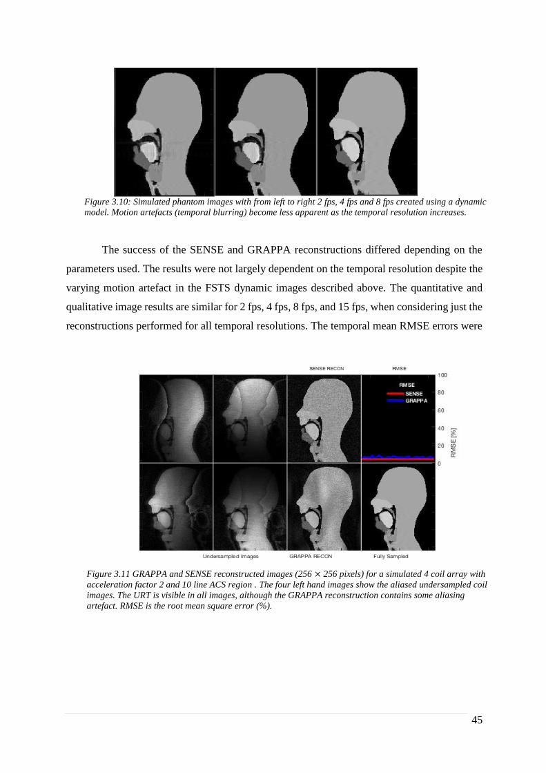
2 |

45

The success of the SENSE and GRAPPA reconstructions differed depending on the

parameters used. The results were not largely dependent on the temporal resolution despite the

varying motion artefact in the FSTS dynamic images described above. The quantitative and

qualitative image results are similar for 2 fps, 4 fps, 8 fps, and 15 fps, when considering just the

reconstructions performed for all temporal resolutions. The temporal mean RMSE errors were

Figure 3.10: Simulated phantom images with from left to right 2 fps, 4 fps and 8 fps created using a dynamic

model. Motion artefacts (temporal blurring) become less apparent as the temporal resolution increases.

Figure 3.11 GRAPPA and SENSE reconstructed images (256 × 256 pixels) for a simulated 4 coil array with

acceleration factor 2 and 10 line ACS region . The four left hand images show the aliased undersampled coil

images. The URT is visible in all images, although the GRAPPA reconstruction contains some aliasing

artefact. RMSE is the root mean square error (%).

2 |

46

fairly consistent, with only those at 15 fps being marginally worse. This may be due to its k-

space only being comprised from two segments, and two phantom dynamic phantom k-spaces.

The GRAPPA reconstructions were fairly dependent on the size of the ACS, again as one would

expect. At an acceleration rate of 2 and 10 ACS lines (of 256 PE lines), resultant images were

consistent for all temporal resolutions: for 2 coils the RMSE was poor (approx. 14%) with

significant aliasing artefacts apparent although the velum and tongue are discernible, whilst for

4 and 8 coils the RMSEs were satisfactory (4-7%) and the reconstructed images are

diagnostically useful with the URT clearly visible, although some aliasing artefacts did remain

outside the region of interest. The SENSE reconstructions for these same parameters were

successful with no additional artefacts when compared to the fully sampled temporally-

segmented dynamic images. An example with 8 fps can be seen in figure 3.11 with 4 coils. As

the ACS region increases in size, it infers that there is more training data for the kernels, and

thus one would expect the reconstructions to be more successful. This was shown in the results

as: for an ACS region of 20 and 40 lines, artefacts were not apparent and the RMSE are only

Figure 3.12 GRAPPA and SENSE reconstructions for a simulated 8 coil array with acceleration factor 2 and

a 40 line ACS region. The eight left hand images show the aliased undersampled coil images. Both SENSE and

GRAPPA reconstructions allow the URT to be fully distinguishable with a low RMSE (< 5%) for all time

points. RMSE is the root mean square error (%).

2 |

47

marginally worse than those for SENSE. An example with 40 ACS lines, 8 coils at 8 fps can be

seen in Figure 3.12.

Increasing the acceleration rate hindered the ability of both the SENSE and GRAPPA

reconstruction techniques ability to retrieve un-aliased images, as one would expect from

theory.19 Only 8 coil reconstructions with accelerations rates greater than 2 were included as

the reconstructions could not be completed for 2 and 4 coils as they were not sufficiently

constrained. All accelerations rates greater than 2 were unable to reproduce un-aliased images,

although this does not necessarily mean they would be completely non-diagnostic. At

acceleration rate 4, the SENSE images had two overlapping repetitions of the image, but as the

URTs are not overlapping one can still determine the URT and the velum and tongue (Figure

3.13). At acceleration rate of 4, with 20 ACS lines, the GRAPPA image were indecipherable

with a RMSE of 92%, and even with 40 ACS lines there is significant noise and aliased image

visible, although the tongue and velum are discernible even if the latter is lost somewhat in the

noisy artefact. At acceleration rate 8, as seen in Figure 3.14, neither the GRAPPA nor SENSE

images were diagnostically useful, with the former indecipherable and the latter showing too

many alias repetitions to provide any useful diagnostic information.

Figure 3.13 GRAPPA and SENSE reconstructions for a simulated 8 coil array with acceleration factor 4 and a

40 line ACS region. The eight left hand images show the aliased undersampled coil images. The SENSE

reconstruction shows two clear alias repetitions although the tongue and velum are still distinguishable. The

GRAPPA reconstruction contains some aliasing artefact as well significant noise, including around the velum

although the majority of the URT is visible. RMSE is the root mean square error (%).

2 |

48

3.3 Testing and Implementation: Conclusion

As a proof of concept, these two initial investigations were a success:

In the non-Cartesian investigation, images comparable to those produced clinically were

produced for both spiral and radial sampling trajectories, including typical artefacts for fully

sampled images. The acceleration of radial sampling also lead to images with artefacts

comparable to those reported in the literature.16-18 This is useful for the prediction of radial and

spiral undersampled image aliasing artefacts, which would allow clinicians to assess whether

particular non-Cartesian sampling trajectories can be used for diagnostic purposes without

reconstruction methods such as GRAPPA and SENSE. However, this investigation used only

examples from a single time point from the phantom, and to fully assess the potential of non-

Cartesian imaging would require through time sampling such as that implemented in Section

3.2.2.1.

In the second investigation, GRAPPA and SENSE reconstructions were carried out for

undersampled multi-coil k-spaces derived from the phantom. Additionally, the ability to

reconstruct un-aliased images was in accordance with theory of the solvability of independent

simultaneous equations (as explained in section 1.5.2), as well as what has been reported in the

Figure 3.14 GRAPPA and SENSE reconstructions for a simulated 8 coil array with acceleration factor 8 and

a 20 line ACS region. The eight left hand images show the aliased undersampled coil images. The SENSE and

GRAPPA reconstructions have too much aliasing artefact for any useful diagnostic information to be

discernible. RMSE is the root mean square error (%).

2 |

49

literature. 19,20 A further test of the applicability of the phantom to test PI reconstructions would

be to perform the same processing and analysis on clinical undersampled MR images and

compare them to the phantom derived reconstructions.

4 Conclusion

The software developing framework, shown in Figure 2.1, has been successfully implemented

to produce the first iteration of a numerical phantom for simulating dynamic speech MR images

using different k-space sampling trajectories. Segmented masks for speech organs of interest

were created and were enhanced using morphological processes. These masks were then

interpolated through time to produce a dynamic phantom of speech, as described in Section 2.

The investigations of non-Cartesian and reconstructed accelerated PI in Section 3 were both

successful proofs of concept, suggesting this phantom model should be further improved to

fully develop its clinical usefulness.

The iterative software engineering framework allows for improvements to be implemented into

each iteration. Initially, an extension to other MRI methodologies would be useful. A first step

would be to attempt to increase the temporal resolution of the segmented images up to 20 fps,

which will allow the sampled k-space interpolated to be increased to 60 fps (16.7 ms temporal

resolution), allowing simulation of single shot imaging such as EPI. The addition of other test

cases such as radial and spiral GRAPPA and SENSE seem another logical extension, after the

experience gained from the two investigations in Section 3. The use of the hybrid EPI images

would also be investigated.15 Through time GRAPPA (k-t GRAPPA), where kernels are

calculated not only from all coils but also across adjacent sampling times, would also be valid

extension to this model.21

In order to better consider Cartesian sampling trajectories, such as high-low used for multi shot

techniques like TSE, relaxation information would need to be incorporated in the model. In

order to achieve this, T1 and T2 would need to be quantified and relaxation maps created. The

organs of interest would be segmented and the corresponding regions of interest of the map

could then be averaged to create a single pair of relaxation parameters for each of the masks.

From a software usability perspective, a desired future iteration of this project would see all

processes combined into a single graphical user interface. This would allow a user to select the

type of k-space sampling trajectory, temporal resolution of the dynamic series, size of image

and k-space matrices amongst others. If applicable the amount of undersampling required would

2 |

50

also be selected, in addition the choice of accelerated PI reconstruction method (GRAPPA or

SENSE). The author would then seek to make this package available to the wider speech MRI

community under a creative commons license.

5 References

1. Canny J. A computational approach to edge detection. IEEE Trans Pattern Anal Mach Intell.

1986(6):679-698.

2. Huang F, Akao J, Vijayakumar S, Duensing GR, Limkeman M. K‐ t GRAPPA: A k‐space

implementation for dynamic MRI with high reduction factor. Magnetic Resonance in Medicine.

2005;54(5):1172-1184.

3. Ball MJ, Rahilly J. Phonetics—the science of speech. 2000.

4. Lingala SG, Sutton BP, Miquel ME, Nayak KS. Recommendations for real‐time speech MRI.

Journal of Magnetic Resonance Imaging. 2016;43(1):28-44.

5. Scott AD, Wylezinska M, Birch MJ, Miquel ME. Speech MRI: Morphology and function. Physica

Medica. 2014;30(6):604-618.

6. Fry DB. The physics of speech. Cambridge University Press; 1979.

7. Cleft Registry And Reporting Network. Table 2: Births by cleft type 2006-2016. https://www.crane-

database.org.uk/?!.iD=eCq. Accessed 07/12, 2017.

8. Colbert S, Green B, Brennan P, Mercer N. Contemporary management of cleft lip and palate in the

united kingdom. have we reached the turning point? British Journal of Oral and Maxillofacial Surgery.

2015;53(7):594-598.

9. Damico JS, Müller N, Ball MJ. The handbook of language and speech disorders. Vol 28. John Wiley

& Sons; 2010.

10. Darley FL, Aronson AE, Brown JR. Motor speech disorders. Saunders; 1975.

11. Hanson EK, Yorkston KM, Britton D. Dysarthria in amyotrophic lateral sclerosis: A systematic

review of characteristics, speech treatment, and augmentative and alternative communication options.

Journal of Medical Speech-Language Pathology. 2011;19(3):12.

12. Bettens K, Wuyts FL, Van Lierde KM. Instrumental assessment of velopharyngeal function and

resonance: A review. J Commun Disord. 2014;52:170-183.

13. Ferreira GZ, Dutka, Jeniffer de Cássia Rillo, Whitaker ME, Souza, Olivia Mesquita Vieira de,

Marino, Viviane Cristina de Castro, Pegoraro-Krook MI. Nasoendoscopic findings after primary palatal

surgery: Can the furlow technique result in a smaller velopharyngeal gap? . 2015;27(4):365-371.

14. Cuadros L. DM lateral digital fluoroscopy. New Mexico: New Mexico Cleft Palate Center; 2009.

15. Sell D, Pereira V, Howard S, Lohmander A. Instrumentation in the analysis of the structure and

function of the velopharyngeal mechanism. Cleft Palate Speech: assessment and intervention. 2012:145-

166.

16. Scott A, Boubertakh R, Birch M, Miquel M. Towards clinical assessment of velopharyngeal closure

using MRI: Evaluation of real-time MRI sequences at 1.5 and 3 T. Br J Radiol. 2012;85(1019):e1083-

e1092.

17. Beer AJ, Hellerhoff P, Zimmermann A, et al. Dynamic near‐real‐time magnetic resonance

imaging for analyzing the velopharyngeal closure in comparison with videofluoroscopy. Journal of

Magnetic Resonance Imaging. 2004;20(5):791-797.

2 |

51

18. Narayanan S, Nayak K, Lee S, Sethy A, Byrd D. An approach to real-time magnetic resonance

imaging for speech production. J Acoust Soc Am. 2004;115(4):1771-1776.

19. Freitas AC, Wylezinska M, Birch MJ, Petersen SE, Miquel ME. Comparison of cartesian and non-

cartesian real-time MRI sequences at 1.5 T to assess velar motion and velopharyngeal closure during

speech. PloS one. 2016;11(4):e0153322.

20. Ettema SL, Kuehn DP, Perlman AL, Alperin N. Magnetic resonance imaging of the levator veli

palatini muscle during speech. The Cleft palate-craniofacial journal. 2002;39(2):130-144.

21. Perry JL, Kuehn DP, Wachtel JM, Bailey JS, Luginbuhl LL. Using magnetic resonance imaging for

early assessment of submucous cleft palate: A case report. The Cleft Palate-Craniofacial Journal.

2012;49(4):e35-e41.

22. Tian W, Yin H, Redett RJ, et al. Magnetic resonance imaging assessment of the velopharyngeal

mechanism at rest and during speech in chinese adults and children. Journal of Speech, Language, and

Hearing Research. 2010;53(6):1595-1615.

23. Bernstein MA, King KF, Zhou XJ. Handbook of MRI pulse sequences. Elsevier; 2004.

24. Wissmann L, Santelli C, Segars WP, Kozerke S. MRXCAT: Realistic numerical phantoms for

cardiovascular magnetic resonance. J Cardiovasc Magn Reson. 2014;16(1):63.

25. Smith MR, Chen L, Hui Y, Mathews T, Yang J, Zeng X. Alternatives to the use of the DFT in MRI

and spectroscopic reconstructions. Int J Imaging Syst Technol. 1997;8(6):558-564.

26. Van de Walle R, Barrett HH, Myers KJ, et al. Reconstruction of MR images from data acquired on

a general nonregular grid by pseudoinverse calculation. IEEE Trans Med Imaging. 2000;19(12):1160-

1167.

27. Gach HM, Tanase C, Boada F. 2D & 3D shepp-logan phantom standards for MRI. . 2008:521-526.

28. Baert A. Parallel imaging in clinical MR applications. Springer Science & Business Media; 2007.

29. McRobbie DW, Moore EA, Graves MJ, Prince MR. MRI from picture to proton. Cambridge

university press; 2007.

30. Robson PM, Grant AK, Madhuranthakam AJ, Lattanzi R, Sodickson DK, McKenzie CA.

Comprehensive quantification of signal‐to‐noise ratio and g‐factor for image‐based and k‐

space‐based parallel imaging reconstructions. Magnetic resonance in medicine. 2008;60(4):895-907.

31. Pruessmann KP, Weiger M, Scheidegger MB, Boesiger P. SENSE: Sensitivity encoding for fast

MRI. Magn Reson Med. 1999;42(5):952-962.

32. Elster AD. MRI questions website. http://www.mriquestions.com/index.html. Updated 2017.

33. Griswold MA, Jakob PM, Heidemann RM, et al. Generalized autocalibrating partially parallel

acquisitions (GRAPPA). Magnetic resonance in medicine. 2002;47(6):1202-1210.

34. Blaimer M, Breuer F, Mueller M, Heidemann RM, Griswold MA, Jakob PM. SMASH, SENSE,

PILS, GRAPPA: How to choose the optimal method. Topics in Magnetic Resonance Imaging.

2004;15(4):223-236.

35. Wright KL, Hamilton JI, Griswold MA, Gulani V, Seiberlich N. Non‐Cartesian parallel imaging

reconstruction. Journal of Magnetic Resonance Imaging. 2014;40(5):1022-1040.

36. Medicines and Healthcare products Regulatory Agency. Safety guidelines for magnetic resonance

imaging equipment in clinical use. . 2015.

37. Bae Y, Kuehn DP, Conway CA, Sutton BP. Real-time magnetic resonance imaging of

velopharyngeal activities with simultaneous speech recordings. The Cleft Palate-Craniofacial Journal.

2011;48(6):695-707.

38. Lauterbur P. Image formation by induced local interactions: Examples employing nuclear magnetic

resonance. . 1973.

2 |

52

39. Ganney P, Maw P, White M. Modernising scientific careers: The ICT competencies. 1st Editiom ed.

UCH Medical Physics and Biomedical Engineering; 2017.

40. Ruthven M, Freitas A, Keevil S, Miquel M. Real-time speech MRI: What is the optimal temporal

resolution for clinical velopharyngeal closure assessment? . 2016;24:(3208.).

41. Prewitt JM. Object enhancement and extraction. Picture processing and Psychopictorics.

1970;10(1):15-19.

42. G. Deng. A generalized unsharp masking algorithm. IEEE Transactions on Image Processing.

2011;20(5):1249-1261.

43. Canny J. A computational approach to edge detection. IEEE Trans Pattern Anal Mach Intell.

1986(6):679-698.

44. Gonzalez RC, Woods RE. Chapter 9: Morphological image processes. In: Digital image processing.

2nd Edition ed. Pearson; 2002:519.

45. Gonzalez RC, Woods RE. Chapter 10: Image segmentation. In: Digital image processing. ;

2002:567.

46. Horn RA. The hadamard product. . 1990;40:87-169.

47. Barron JL, Fleet DJ, Beauchemin SS. Performance of optical flow techniques. International journal

of computer vision. 1994;12(1):43-77.

48. Rueckert D, Sonoda LI, Hayes C, Hill DL, Leach MO, Hawkes DJ. Nonrigid registration using free-

form deformations: Application to breast MR images. IEEE Trans Med Imaging. 1999;18(8):712-721.

49. Sven. InterpMask matlab function. 2014. URL:// https://uk.mathworks.com/matlabcentral/...

fileexchange/46429-interpmask-interpolate--tween--logical-masks?requestedDomain=true

50. Zou KH, Warfield SK, Bharatha A, et al. Statistical validation of image segmentation quality

based on a spatial overlap index. Acad Radiol. 2004;11(2):178-189.

51. Fessler JA. On NUFFT-based gridding for non-cartesian MRI. Journal of Magnetic Resonance.

2007;188(2):191-195.

52. Greengard L, Lee J. Accelerating the nonuniform fast fourier transform. SIAM Rev. 2004;46(3):443-

454.

53. Liu F, Velikina JV, Block WF, Kijowski R, Samsonov AA. Fast realistic MRI simulations based on

generalized multi-pool exchange tissue model. IEEE Trans Med Imaging. 2017;36(2):527-537.

54. Uecker M, Ong F, Tamir JI, et al. Berkeley advanced reconstruction toolbox. 2015;23:2486.

55. Pauly JM. Gridding & the NUFFT for non-cartesian image reconstruction. . 2013:45.

56. Patch SK. K-space data preprocessing for artifact reduction in MR imaging. . 2005:73-87.

57. Glover GH, Pauly JM. Projection reconstruction techniques for reduction of motion effects in MRI.

Magnetic resonance in medicine. 1992;28(2):275-289.

58. Peters DC, Rohatgi P, Botnar RM, Yeon SB, Kissinger KV, Manning WJ. Characterizing radial

undersampling artifacts for cardiac applications. Magnetic resonance in medicine. 2006;55(2):396-403.