Department of Materials Science and Engineering p. 36-1...
11
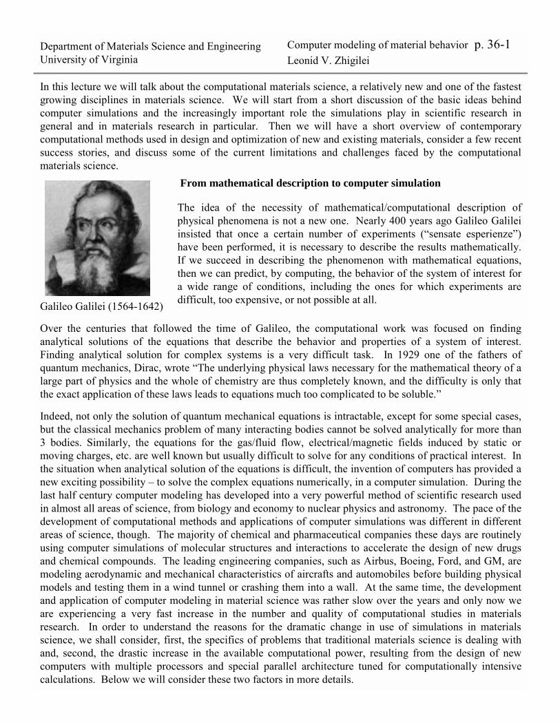
Department of Materials Science and Engineering University of Virginia Computer modeling of material behavior p. 36-1 Leonid V. Zhigilei In this lecture we will talk about the computational materials science, a relatively new and one of the fastest growing disciplines in materials science. We will start from a short discussion of the basic ideas behind computer simulations and the increasingly important role the simulations play in scientific research in general and in materials research in particular. Then we will have a short overview of contemporary computational methods used in design and optimization of new and existing materials, consider a few recent success stories, and discuss some of the current limitations and challenges faced by the computational materials science. From mathematical description to computer simulation The idea of the necessity of mathematical/computational description of physical phenomena is not a new one. Nearly 400 years ago Galileo Galilei insisted that once a certain number of experiments (sensate esperienze) have been performed, it is necessary to describe the results mathematically. If we succeed in describing the phenomenon with mathematical equations, then we can predict, by computing, the behavior of the system of interest for a wide range of conditions, including the ones for which experiments are difficult, too expensive, or not possible at all. Over the centuries that followed the time of Galileo, the computational work was focused on finding analytical solutions of the equations that describe the behavior and properties of a system of interest. Finding analytical solution for complex systems is a very difficult task. In 1929 one of the fathers of quantum mechanics, Dirac, wrote The underlying physical laws necessary for the mathematical theory of a large part of physics and the whole of chemistry are thus completely known, and the difficulty is only that the exact application of these laws leads to equations much too complicated to be soluble. Indeed, not only the solution of quantum mechanical equations is intractable, except for some special cases, but the classical mechanics problem of many interacting bodies cannot be solved analytically for more than 3 bodies. Similarly, the equations for the gas/fluid flow, electrical/magnetic fields induced by static or moving charges, etc. are well known but usually difficult to solve for any conditions of practical interest. In the situation when analytical solution of the equations is difficult, the invention of computers has provided a new exciting possibility to solve the complex equations numerically, in a computer simulation. During the last half century computer modeling has developed into a very powerful method of scientific research used in almost all areas of science, from biology and economy to nuclear physics and astronomy. The pace of the development of computational methods and applications of computer simulations was different in different areas of science, though. The majority of chemical and pharmaceutical companies these days are routinely using computer simulations of molecular structures and interactions to accelerate the design of new drugs and chemical compounds. The leading engineering companies, such as Airbus, Boeing, Ford, and GM, are modeling aerodynamic and mechanical characteristics of aircrafts and automobiles before building physical models and testing them in a wind tunnel or crashing them into a wall. At the same time, the development and application of computer modeling in material science was rather slow over the years and only now we are experiencing a very fast increase in the number and quality of computational studies in materials research. In order to understand the reasons for the dramatic change in use of simulations in materials science, we shall consider, first, the specifics of problems that traditional materials science is dealing with and, second, the drastic increase in the available computational power, resulting from the design of new computers with multiple processors and special parallel architecture tuned for computationally intensive calculations. Below we will consider these two factors in more details. Galileo Galilei (1564-1642)
Transcript of Department of Materials Science and Engineering p. 36-1...
Department of Materials Science and EngineeringUniversity of Virginia
Computer modeling of material behavior p. 36-1Leonid V. Zhigilei
In this lecture we will talk about the computational materials science, a relatively new and one of the fastest growing disciplines in materials science. We will start from a short discussion of the basic ideas behind computer simulations and the increasingly important role the simulations play in scientific research in general and in materials research in particular. Then we will have a short overview of contemporary computational methods used in design and optimization of new and existing materials, consider a few recent success stories, and discuss some of the current limitations and challenges faced by the computational materials science.
From mathematical description to computer simulation
The idea of the necessity of mathematical/computational description of physical phenomena is not a new one. Nearly 400 years ago Galileo Galileiinsisted that once a certain number of experiments (�sensate esperienze�) have been performed, it is necessary to describe the results mathematically. If we succeed in describing the phenomenon with mathematical equations, then we can predict, by computing, the behavior of the system of interest for a wide range of conditions, including the ones for which experiments are difficult, too expensive, or not possible at all.
Over the centuries that followed the time of Galileo, the computational work was focused on finding analytical solutions of the equations that describe the behavior and properties of a system of interest. Finding analytical solution for complex systems is a very difficult task. In 1929 one of the fathers of quantum mechanics, Dirac, wrote �The underlying physical laws necessary for the mathematical theory of a large part of physics and the whole of chemistry are thus completely known, and the difficulty is only that the exact application of these laws leads to equations much too complicated to be soluble.�
Indeed, not only the solution of quantum mechanical equations is intractable, except for some special cases, but the classical mechanics problem of many interacting bodies cannot be solved analytically for more than 3 bodies. Similarly, the equations for the gas/fluid flow, electrical/magnetic fields induced by static or moving charges, etc. are well known but usually difficult to solve for any conditions of practical interest. In the situation when analytical solution of the equations is difficult, the invention of computers has provided a new exciting possibility � to solve the complex equations numerically, in a computer simulation. During the last half century computer modeling has developed into a very powerful method of scientific research used in almost all areas of science, from biology and economy to nuclear physics and astronomy. The pace of the development of computational methods and applications of computer simulations was different in different areas of science, though. The majority of chemical and pharmaceutical companies these days are routinely using computer simulations of molecular structures and interactions to accelerate the design of new drugs and chemical compounds. The leading engineering companies, such as Airbus, Boeing, Ford, and GM, are modeling aerodynamic and mechanical characteristics of aircrafts and automobiles before building physical models and testing them in a wind tunnel or crashing them into a wall. At the same time, the development and application of computer modeling in material science was rather slow over the years and only now we are experiencing a very fast increase in the number and quality of computational studies in materials research. In order to understand the reasons for the dramatic change in use of simulations in materials science, we shall consider, first, the specifics of problems that traditional materials science is dealing with and, second, the drastic increase in the available computational power, resulting from the design of new computers with multiple processors and special parallel architecture tuned for computationally intensive calculations. Below we will consider these two factors in more details.
Galileo Galilei (1564-1642)

Department of Materials Science and EngineeringUniversity of Virginia
Computer modeling of material behavior p. 36-2Leonid V. Zhigilei
Characteristic length- and time-scales in materials modeling
As you learned in the previous lectures, real materials have many defects, including vacancies, impurities, dislocations, grain boundaries, domain walls (in magnetic and ferroelectric materials), etc. It is the structure and properties of the defects, their interactions, and their thermodynamics that define the macroscopic properties of real materials. The totality of all lattice defects is called microstructure of the specimen. You have also learned that the microstructure can be changed/controlled by thermal or mechanical processing. Therefore, investigation of the structure, properties and interactions of defects, their evolution during processing and their response to the external conditions is in the core of materials research.
While some of the most fundamental questions concerning the behavior and interaction of defects still remain unresolved, the application of computational methods to address this questions has been rather limited. The lack of computational activities in this area can be attributed to the fact that lattice defects belong to the intermediate (or �mesoscopic�) length-scale. They are �too big� to be simulated by atomic-level computational models, commonly used in chemistry, and, at the same time, they are �too small� to for macroscopic continuum modeling, used in engineering. While atomistic and continuum simulation techniques are well established and extensively used, the mesoscopic modeling is still in its infancy. The development of mesoscopic models is hampered by insufficient understanding of the microscopic properties and behavior of defects. Only now a quickly growing computational power of modern computers is reaching the level that allows one to perform realistic atomic-level analysis of lattice defects and their interactions. The insights extracted from such simulations are used as input for the development and parameterization of computational models for mesoscopic simulations. The range of time and length scales relevant to different materials science problems is illustrated in a schematic drawing in the next page.
Growth of the computational power. Moore’s law.As discussed above, it is the steep and steady increase in the available computational power that is responsible for the current fast development of the computational materials science. Gordon Moore, co-founder of Intel, noted in 1965 that that the number of transistors per square inch on integrated circuits (and computational speed) had doubled every year since the integrated circuit was invented. Moore predicted that this trend would continue for the foreseeable future. Currently it is expected that the Moore's Law will hold for at least another two decades.
The figure to the left shows �ASCI White�, the RS/6000 SP supercomputer developed by IBM and installed at the LLNL in 2001, is considered to be the world's fastest supercomputer. It covers an area the size of two basketball courts and is mostly used by the DOE for computations related to the safety and reliability of the US nuclear weapons stockpile. Some of the record-breaking materials science � related simulations discussed below have been performed on this computer.

Department of Materials Science and EngineeringUniversity of Virginia
Computer modeling of material behavior p. 36-3Leonid V. Zhigilei
Mac
rosc
opic
10-9
10-8
10-7
Leng
th S
cale
, met
ers
10
-3
103
106
109
Leng
th S
cale
, num
ber o
f ato
ms
1021
10-1
210
-910
-7Ti
me
Scal
e, se
cond
s
1
Mes
osco
pic
Mo Li, JHU, Atomistic model of a nanocrystalline
Vasily Bulatov et al., LLNLDislocation dynamics simulation
Farid Abraham et al., IBMAtomistic simulation of crack propagation
Ato
mis
tic /
Nan
osco
pic
Leonid Zhigilei et al., UVaPhase transformation on diamond surfaces
Elizabeth Holm, SandiaSimulation of intergranular fracture
Monte Carlo Potts model
Continuum, macroscopic modeling constitutive relations
Length- and time-scales in materials modeling

Department of Materials Science and EngineeringUniversity of Virginia
Computer modeling of material behavior p. 36-4Leonid V. Zhigilei
Atomic-level simulations: Molecular Dynamics
Molecular dynamics is a computer simulation technique that allows one to predict the time evolution of a system of interacting particles (atoms, molecules, granules, etc.). The basic idea is very simple:
! First, for a system of interest, one has to specify a set of initial conditions (e.g. initial positions and velocities of all particles in the system) and interaction potential (energy of the system as a function of atomic positions). The forces among all the atoms can be derived from the interaction potential.
! Second, the evolution of the system in time can be followed by solving a set of classical equations of motion for all particles in the system. Within the framework of classical mechanics, the equations that govern the motion of classical particles are the ones that correspond to the second law of classical mechanics formulated by Sir Isaac Newton over 300 years ago:
Fdt
rdmor Fdtvdmor Fam i2
i2
iii
iiii
rrrrrr ===
If the particles of interest are atoms, and if there are a total of Nat of them in the system, the force acting on the ith atom at a given time can be obtained from the interatomic potential V(r1, r2, r3, �, rNat) that, in general, is a function of the positions of all the atoms, )r,...,r,r,rV(- F
atN321iirrrrrr
∇=
Once the initial conditions and the interaction potential are defined, the equations of motion can be solved numerically. The simplest but not very accurate method that can be used to solve the equations is so-called Euler�s method:If we know the positions and velocities of all particles in a system at time t, , we can find the positions and velocities at time t + ∆t:
( ) ( )tv ,tr iirr
Distance between atoms, rij, Å
Ener
gy,e
V,Fo
rce,
eV/Å
2 4 6 8
-0.01
-0.005
0
0.005
12
1221 dr
)V(r- F F =−=rr
2112 rrr rr −=
12 1Fr
2Fr
The result of the solution are the positions and velocities of all the atoms as a function of time.
For example, if we only have 2 atoms in a system (e.g. a diatomic molecule), the potential depends only on the distance between the two atoms V(r12):
Force
Energy
∆tv(t)r(t)∆t)r(t +=+∆t
mF(t) v(t)∆t a(t)v(t)∆t)v(t +=+=+
repulsion attraction
Department of Materials Science and EngineeringUniversity of Virginia
Computer modeling of material behavior p. 36-5Leonid V. Zhigilei
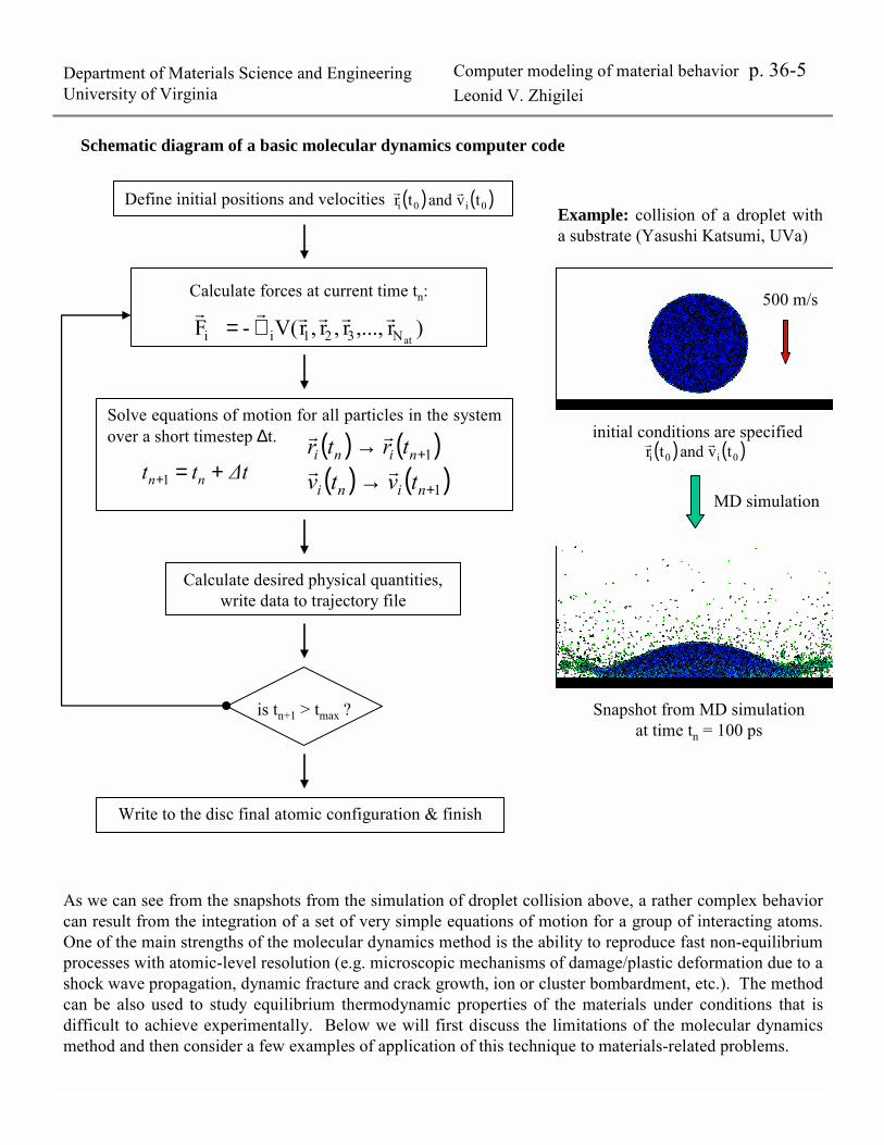
Schematic diagram of a basic molecular dynamics computer code
Define initial positions and velocities
Calculate forces at current time tn:
Solve equations of motion for all particles in the system over a short timestep ∆t. ( ) ( )1+→ nini trtr rr
Calculate desired physical quantities, write data to trajectory file
)r,...,r,r,rV(- FatN321ii
rrrrrr∇=
( ) ( )1+→ nini tvtv rr∆ttt nn +=+1
is tn+1 > tmax ?
Write to the disc final atomic configuration & finish
( ) ( )0i0i tv and tr rr
initial conditions are specified( ) ( )0i0i tv and tr rr
500 m/s
MD simulation
Snapshot from MD simulation at time tn = 100 ps
Example: collision of a droplet with a substrate (Yasushi Katsumi, UVa)
As we can see from the snapshots from the simulation of droplet collision above, a rather complex behavior can result from the integration of a set of very simple equations of motion for a group of interacting atoms. One of the main strengths of the molecular dynamics method is the ability to reproduce fast non-equilibrium processes with atomic-level resolution (e.g. microscopic mechanisms of damage/plastic deformation due to a shock wave propagation, dynamic fracture and crack growth, ion or cluster bombardment, etc.). The method can be also used to study equilibrium thermodynamic properties of the materials under conditions that is difficult to achieve experimentally. Below we will first discuss the limitations of the molecular dynamics method and then consider a few examples of application of this technique to materials-related problems.

Department of Materials Science and EngineeringUniversity of Virginia
Computer modeling of material behavior p. 36-6Leonid V. Zhigilei
Limitations of the molecular dynamics method
As soon as you have a computer code that is working, there is a temptation to immediately apply it to a wide range of problems. It is very important, however, to clearly understand the approximations that were used in designing the mathematical model and the related limitations of the computational technique. It is not unusual for mathematical modeling to be misused by being applied to the phenomena that lays outside the domain for which the model was developed. Confusing or simply wrong results can be obtained (and occasionally published) in these cases. It is, therefore, very important to understand the limitations of computational models. In particular, the main limitations of the classical molecular dynamics simulation technique are listed below.
1. Classical description of interatomic interaction. In a molecular dynamics simulation electrons are not present explicitly, they are introduced through the potential energy that is a function of atomic positions only (this is called Born-Oppenheimer approximation in quantum mechanics). The potential energy, in turn, is approximated by an analytic function that gives the potential energy U as a function of atomic positions. As you remember, we need the potential energy to calculate forces, that are obtained as a gradient of a potential energy function. Design of the potential function and choice of the parameters is often based on fitting to available experimental data (e.g. equilibrium geometry of stable phases, cohesive energy, elastic moduli, vibrational frequencies, temperatures of the phase transitions, etc.). If the potential is designed based on one set of properties, it may not work well in the description of other properties that were not included in the parameterization�
2. Classical description of atomic motion. In classical molecular dynamics we replace Schrödinger equation for nuclei with classical Newton equation. Quantum mechanical analysis suggests that the wave nature of electrons dominates over the particle behavior, and electrons can not be considered within classical approximation. At the same time, all atoms, except for the lightest ones such as H, He, Ne, can be considered as �point� particles at sufficiently high temperature and classical mechanics can be used to describe their motion.
3. Time- and length-scale limitations. The fact that in a molecular dynamics simulation we have to integrate the equations of motion for all atoms in a system puts severe limitations on the number of atoms that can be included in the simulation and the time of the simulation. These limitations constrain the range of problems that can be addressed by the method.
Time-scale: The maximum timestep of integration in a molecular dynamics simulation is defined by the fastest motion in the system. The period of vibrational motion of atoms in a solid is typically on the order of hundreds femtoseconds (1 fs = 10-15 s) to picoseconds (1 ps = 10-12 s). Therefore, a typical timestep in the simulation cannot be longer than a femtosecond. Using modern computers it is possible to calculate 106 �108 timesteps. Therefore we can only simulate processes that occur within 1 � 100 ns. This is a serious limitation for many problems that involve diffusion, cluster/vapor film deposition, relaxation of irradiation damage, and other processes that occur at a longer time-scale.
Length-scale: The size of the computational cell is limited by the number of atoms that can be included in the simulation, typically 104 � 107. This corresponds to the size of the computational cell on the order of tens of nm. Any structural features of interest and spatial correlation lengths in the simulation should be smaller than the size of the computational cell. To make sure that the finite size of the computational cell does not introduce any artifacts into the simulation results, one can perform simulations for systems of different size and compare the measured properties.

Department of Materials Science and EngineeringUniversity of Virginia
Computer modeling of material behavior p. 36-7Leonid V. Zhigilei
Dealing with the time- and length-scale limitations of the molecular dynamics method
Due to the limitations on the size of the system that can be simulated, an important aspect of any molecular dynamics simulation is an adequate description of the �interaction� of atoms in the system (sometimes called �computational cell�) with surrounding �infinite� material. We have to define boundary conditions and apply special methods for temperature and pressure control in the molecular dynamics computational cell (heat and work exchange between the molecular dynamics computational cell and the surroundings).
MD
Large external system
MD
Large external system
surface
The record-breaking simulations are:Record time scale � protein folding simulation. Simulation of 1 microsecond of folding of a small, 36 amino-acid, protein with surrounding water molecules (12,000 atoms total) took ~3 months of dedicated computing using all 256 processors of CRAY-T3E supercomputer at Pittsburgh Supercomputer Center. Timestep of 2 fs was used → 1µs = 5×10⁸ steps of integration.Record length scale � multi-billion simulations of crystal fracture, discussed in the next page.

Department of Materials Science and EngineeringUniversity of Virginia
Computer modeling of material behavior p. 36-8Leonid V. Zhigilei
Current applications of the MD simulation technique in materials science include investigations of point, linear, and planar defects in crystals and their interactions, microscopic mechanisms of fracture, surface reconstruction, melting and faceting, film growth, friction, surface modification by ion or cluster bombardment, etc.
Nano-jet implantation of functional molecules into a polymer substrate [Masahiro Goto et al., J. Appl. Phys. 90, 4755-4760, 2001]
Shockwave-induced plasticity[B.L. Holian and P.S. Lomdahl,
Science 280, 2085 (1998)]
Current state of the art (length-scale): billions of atoms
Billion atoms simulation of work-hardening and ductile failure of a FCC solid under tension. The system is a FCC crystallite with the total number of atoms of 1,023,103,872. The total simulation time is 200,000 timesteps. It takes 1.7 seconds per timestep for a 4096-node simulation on ASCI White computer (~four clock-days of total simulation time).
http://www.almaden.ibm.com/st/Simulate/df.html
Test run with 5,180,116,000 particles has been performed in 2000 by J. Roth, F. Gähler, and H.-R.. Trebin[Int. J. Modern Phys. C 11, 317-322, 2000] in Jülich, Germany on 512 processors of Cray-T3E computer. The test run took 40 minutes for 5 timesteps of integration.

Department of Materials Science and EngineeringUniversity of Virginia
Computer modeling of material behavior p. 36-9Leonid V. Zhigilei
Kinetic Monte Carlo method for simulation of slow thermally-activated processes, such as diffusion.
Atom Vacancy
Em
Distance
Energy As you remember from previous lectures, the atomic diffusion is a thermally-activated process. In the case of the vacancy diffusion mechanism this means that in order for an atom to jump into a vacancy site, it needs to overcome a high energy state, when old bonds are already broken and new ones are not formed yet. The probability for an atom to get enough energy for a jump can be described by the Arrhenius equation:
−= Tk
EexpRRB
m0j
where R0 is an attempt frequency proportional to the frequency of atomic vibrations and Em is the diffusion activation energy � height of the barrier.
If we try to study diffusion using molecular dynamics method, the resulting picture will be rather boring � most of the time atoms will spend oscillating around their equilibrium positions, as in the picture on the left side of the page.
The simulation can be significantly accelerated if instead of solving equations of motion, me will directly use the jump rates predicted by the Arrhenius equation. In other words, we will just move atoms randomly from one equilibrium position to another equilibrium position with frequencies that are defined by the energy barriers that separate the equilibrium positions. This idea � to randomly move atoms with the rates defined by the activation barriers � is in the core of the kinetic Monte Carlo method.
The pictures below show the result from kinetic Monte Carlo simulation of island growth on a homogeneous substrate and a substrate with nanoscale patterning. http://www.lce.hut.fi/publications/annual2000/node22.html
MD simulation by T. Kwok, P. S. Ho, and S. Yip. Initial atomic positions are shown by the circles, trajectories of atoms are shown by lines. A region around a grain boundary is shown.
Schematic representation of the vacancy diffusion mechanism
The main limitation of the kinetic Monte Carlo method is that we have to specify all the barriers/rates in advance, before the simulation. As the system becomes more complex, the number of possible events becomes larger and parameterization of the model becomes more difficult�

Department of Materials Science and EngineeringUniversity of Virginia
Computer modeling of material behavior p. 36-10Leonid V. Zhigilei
Dislocation DynamicsAs you remember from the lecture on defects, dislocations are linear defects that are responsible for plastic deformation in crystalline solids. If we understand the dynamics and interaction of dislocations in materials, we will be able to understand and, ultimately, control the mechanical properties (strength and plasticity) of materials. The complexity of a collective behavior of a large number of dislocations in crystals undergoing plastic deformation makes it difficult to provide a complete and consistent theoretical description of plastic deformation. Mesoscopic simulation method of dislocation dynamics provides additional means for checking existing theoretical concepts and development of new ideas in this research area.
The dislocation dynamics model is based on the following ideas:
Spatial discretization: The simulated area is grided with grid size that is larger than the distance of spontaneous annihilation of two dislocations (typically several nanometers).
Dislocation lines are represented by chains of connected dislocation segments. New segments are introduced if two adjacent segments become too long (if the curvature is too crudely described).Forces acting on dislocations are calculated based on the elasticity theory. These forces include forces due to the interaction of the elastic fields of different dislocations, external forces of mechanical loading, etc.
Short-range interactions (reactions) of dislocation cores are described based on the results of molecular dynamics simulations and experimental data.
Equations of motion of dislocations are solved (different methods has been proposed for description of dislocation motion, including �Monte Carlo�-type and �molecular dynamics� �type methods).
Below are a few examples of dislocation dynamics simulations:
Simulation of dislocation networks in relaxed �quantum-dot� structureshttp://www.research.ibm.com/dislocationdynamics/
A nice collection of animations from dislocation dynamics simulations can be found at http://zig.onera.fr/lem/DisGallery/

Department of Materials Science and EngineeringUniversity of Virginia
Computer modeling of material behavior p. 36-11Leonid V. Zhigilei
Finite element method � �continuum� description of materials
! An object is divided into small pieces (like in a Lego game) that are called elements. Each element is defined by nodes.
! A proper behavior is assigned to the elements and physical quantities are defined on each element.
! A system of equations, that describes evolution of quantities in the system of connected elements is solved.
! Quantities of interest (e.g. stress, strain, density, temperature, etc.) are calculated on each element.
Finite element method (FEM) is a very popular computational method that is used in materials science. In the FEM there are no restrictions on the scale of the object (can be large � a wing of an aircraft or a bridge) or small (stress distribution around a tip of a micro-crack or small island on a surface). The FEM method is the most popular simulation method in engineering, it is used in mechanical and aerospace engineering, structural analysis, bioengineering, analysis of fluid flow, etc.
A (very simplified) description of the FEM can be given as follows:
As with any numerical tool, FEM can be easily misused and it is important to understand the limitations of the method. In the case of FEM, the limitations are defined by the physical models that lead to the equations incorporated into the FEM.
http://www.physics.cornell.edu/sethna/teaching/Simulations/FEM.html
Element
Nodes
To learn more about modeling in materials science, check the web page for MSE 524 coursehttp://www.people.virginia.edu/~lz2n/mse524/�and take this class.