WORKING PAPERS

Rod Falveya

Neil Foster b cd

David Greenawaya

North-South Trade, Openness and Growth

June 2001

Working Paper No: 0108

DEPARTMENT OF ECONOMICS

UNIVERSITY OF VIENNAAll our working papers are available at: http://mailbox.univie.ac.at/papers.econ

North-South Trade, Openness and Growth

Rod Falveya

Neil Foster b cd

David Greenawaya

June 2001

ABSTRACT In models of endogenous growth, international trade can impact upon growth by allowing access to the innovative products of other countries. Since developing countries do little if any innovation, it is primarily through trade with developed countries that they profit from higher levels of technological development. In this paper we construct an empirical model to estimate trade flows from the ‘North’ to the ‘South’. Using the results of this model we construct a measure of openness to Northern imports, based on the deviation of actual imports from that predicted by our model. We find that this measure of openness is significantly and robustly related to economic growth, suggesting that trade with advanced countries can facilitate growth through the absorption of advanced technology.

JEL Classification: F14, F43, O40

Keywords: North-South Trade, Openness, Growth

a The University of Nottingham, UniversityPark, Nottingham, NG7 2RD, United Kingdom. b The University of Vienna, Department of Economics, Hohenstaufengasse 9, A1010, Vienna. c Acknowledges funding from the Economic and Social Research Council. d Corresponding author. Email: neil.foster@univie.ac.at

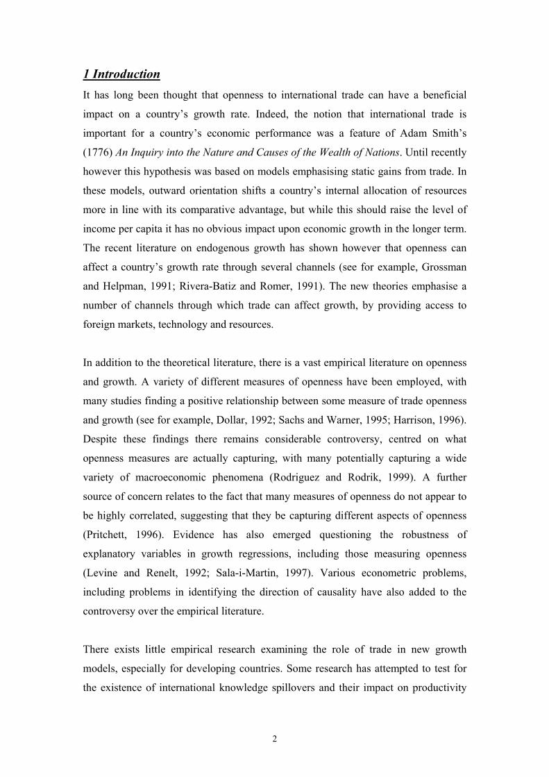
1 Introduction It has long been thought that openness to international trade can have a beneficial

impact on a country’s growth rate. Indeed, the notion that international trade is

important for a country’s economic performance was a feature of Adam Smith’s

(1776) An Inquiry into the Nature and Causes of the Wealth of Nations. Until recently

however this hypothesis was based on models emphasising static gains from trade. In

these models, outward orientation shifts a country’s internal allocation of resources

more in line with its comparative advantage, but while this should raise the level of

income per capita it has no obvious impact upon economic growth in the longer term.

The recent literature on endogenous growth has shown however that openness can

affect a country’s growth rate through several channels (see for example, Grossman

and Helpman, 1991; Rivera-Batiz and Romer, 1991). The new theories emphasise a

number of channels through which trade can affect growth, by providing access to

foreign markets, technology and resources.

In addition to the theoretical literature, there is a vast empirical literature on openness

and growth. A variety of different measures of openness have been employed, with

many studies finding a positive relationship between some measure of trade openness

and growth (see for example, Dollar, 1992; Sachs and Warner, 1995; Harrison, 1996).

Despite these findings there remains considerable controversy, centred on what

openness measures are actually capturing, with many potentially capturing a wide

variety of macroeconomic phenomena (Rodriguez and Rodrik, 1999). A further

source of concern relates to the fact that many measures of openness do not appear to

be highly correlated, suggesting that they be capturing different aspects of openness

(Pritchett, 1996). Evidence has also emerged questioning the robustness of

explanatory variables in growth regressions, including those measuring openness

(Levine and Renelt, 1992; Sala-i-Martin, 1997). Various econometric problems,

including problems in identifying the direction of causality have also added to the

controversy over the empirical literature.

There exists little empirical research examining the role of trade in new growth

models, especially for developing countries. Some research has attempted to test for

the existence of international knowledge spillovers and their impact on productivity

2

growth. Coe and Helpman (1995) and Coe, Helpman and Hoffmaister (1997) for

example, show that there exist knowledge spillovers between countries, with trade

being one mechanism through which such spillovers occur. Such spillovers are found

to occur between developed countries, but also from developed countries to

developing countries. There is however little evidence concerning the role of goods

trade, although Lee (1993, 1995) has shown that restrictions on imports of capital

goods can reduce growth.

This paper examines the impact of goods trade on a country’s growth rate. In

particular we emphasise the role of manufactured imports from developed to

developing countries. We emphasise North-South trade because it is through trade

with developed countries that developing countries should benefit from advanced

technology. Historically a large share of North-South trade has consisted of imports of

manufactured goods, which are likely to embody advanced technology1. This suggests

that it is primarily through North-South trade that developing countries can benefit

from trade through the importation of advanced technology.

The remainder of this paper is organised as follows. In section 2 we develop an

empirical model that predicts trade flows from the ‘North’ to the ‘South’. We show

that the model can explain a large proportion of the cross-country variation in imports

from the North. Using the predicted values from this model we construct a measure of

openness to imports from the North. In section 3 we use this measure to estimate the

impact of openness on the growth rates of our sample of Southern countries. We find

that those countries that are ranked as more open enjoy significantly higher growth

rates than those ranked as closed to Northern imports, a result that appears to be quite

robust. Section 4 provides some overall conclusions.

2 Measuring Openness to Northern Imports 2.1 Background A large number of openness measures have been used in the empirical literature.

Often a summary indicator of trade is employed, for example exports, total trade or

1 Wood (1994) for example, finds that during the period 1955 to 1989 between 73 and 79 percent of the total exports of the North to the South consisted of manufactures.

3

the trade to GDP ratio. Others use data on tariff rates, while some use data on a

number of different indicators to form an index of trade distortions. One shortcoming

of many of these measures is that often they do not relate to the theories linking

growth to trade. The theory emphasises the role of imports, and in particular the role

of imports of capital, intermediates and technology in the growth process. For

developing countries we would expect the benefits to growth of such imports to arrive

through trade with more advanced countries, where most R&D is undertaken.

What we do is construct a measure of openness to the imports of advanced countries

for a sample of developing countries, by estimating an empirical model that predicts

such imports using data on various characteristics of both the importer and exporter.

The extent of deviation of actual trade from that predicted is taken as an indicator of

the extent of trade restrictions on Northern imports. A number of others have

attempted to measure openness in a similar manner, although they tend to look at

exports rather than imports and tend not to concentrate on North-South trade. Chenery

and Syrquin (1989)2 for example measure openness for a sample of up to 108

countries for 1965 and 1980 according to their observed share of merchandise exports

in GDP relative to the predicted share. The predicted share is constructed by adjusting

(in an ad-hoc fashion) for such things as the level of GDP per capita, size, transport

costs and various resource endowments. A high relative export level led to an outward

oriented classification, while a low level resulted in an economy being classed as

inward oriented. They showed that the ranking of countries corresponded fairly well

with that of the World Development Report 1987. Furthermore, they found that GDP

growth was higher in the outward oriented group than in the inward oriented group,

suggesting that openness was good for growth.

Leamer (1988)3 conducts a similar exercise, but bases his measure of openness on a

modified version of the Hecksher-Ohlin-Vanek model of trade flows. He predicts a

country’s net exports as a function of the country’s endowment of land, labour,

capital, oil, coal, minerals, the distance to its markets and the country’s trade balance.

The model is estimated for 1982 on 182 commodities at the 3-digit SITC level. Two

measures of openness are developed, the first is an adjusted trade intensity ratio that

2 See also Chenery and Syrquin (1975). 3 This builds upon Leamer (1984).

4

allows for differences in resource supplies and the second is the ratio of actual to

predicted trade. Leamer states that the first of these is analogous to a measure of

welfare loss, indicating the percentage of GDP lost as a result of trade barriers, while

the second is analogous to a tariff average that suggests how much trade is deterred by

barriers. Leamer appears to be sceptical of the results obtained, questioning whether

the adjusted trade intensity ratio is actually measuring barriers to trade or is more an

indicator of tastes, omitted resources and historical accidents. He does state however

that many of the “unusual aspects of patterns of net exports occur mostly from the

export side and are related to historical factors or to special resources, and not to trade

barriers. It may well be that a separate study of the import side would be productive.”

(p. 179). Since we are considering imports, many of these problems may be

overcome. Furthermore, the fact that we use more aggregated data may remove the

influence of tastes, and also of historical accidents and special resources that result in

some countries specialising in particular commodities.

2.2 Predicting Trade Flows To measure openness in our sample we construct a model that explains the extent of

trade, and in particular imports of manufactured goods from the North. Leamer (1974)

identifies three predictors of imports; resistance, the stage of development and

resource supplies. Resistance includes such things as transport costs and the level of

tariffs and trade restrictions. Transport costs have for a long time been considered an

important determinant of trade. Limao and Venables (1999) have shown that doubling

transport costs can reduce trade flows by around 80 percent. Various proxies are often

used to capture the impact of resistance on trade; these include distance, the presence

of common borders and language and whether countries are landlocked or not. More

recently it has been proposed that the internal infrastructure of both the importer and

exporter may affect the level of trade through its impact on internal transport costs

(for example, Bougheas et al, 1999; Limao and Venables, 1999).

Leamer also suggests that stage of development would affect imports; ceteris paribus

the more developed a country is, the higher are its imports expected to be. A variety

of proxies for stage of development have been suggested in the literature, examples

include the level of GDP and the per capita income. Finally, resource supplies are also

5

considered to be an important determinant of a country’s imports. These include such

things as the stock of capital, the labour force, the level of human capital, the presence

of natural resources and the level of R&D. These factors determine a country’s

comparative advantage and the extent of specialisation, which can then affect the level

of imports.

To predict imports we use a variant of the gravity model that is augmented with

various measures of factor endowments. The use of the gravity model as a means of

estimating trade flows has increased a great deal following the development of a

theoretical foundation for the model by amongst others Anderson (1979), Bergstrand

(1985) and Helpman and Krugman (1985). The model relates a country’s imports,

exports or total trade to the size of the importer and exporter and to the distance

between the two. Trade flows are seen as being the result of supply conditions at the

origin, demand conditions at the destination, and trade stimulating and trade

restricting forces between the two countries. These determinants are usually proxied

respectively by the GDP of the exporter and importer, their per capita incomes and

distance from each other. Trade stimulating forces are other factors that can enhance

trade between countries; examples include common language, preferential trading

arrangements, former colonial ties and direct land borders. Trade restricting forces are

factors that drive a wedge between supply and demand and consist of three elements;

transport costs, transport time (which represents problems of perishability,

adaptability to market conditions and irregularities in supply), and psychic distance

(which represents familiarity with laws, institutions and habits).

Many applied papers4 estimate some variant of the following simple version of the

gravity equation

)()log().log().log()log(

4

321

othersDistGDPCGDPCGDPGDPEX xmmxmxxm

ββββα ++++=

where EXxm are exports from the exporter (x) to the importer (m), GDPx and GDPm are

the gross domestic products of the exporter and importer respectively, GDPCx and

GDPCm are the per capita GDP’s of the exporter and importer respectively and Distxm

is the distance between the importer and exporter. Other variables often included are

6

dummy variables for common languages and common borders, for landlocked

countries and for trade bloc participation. The first is included since it is expected that

being adjacent to another country increases familiarity with the culture, institutions

and preferences of the trade partner, while a common language facilitates

communication between trade partners and reduces the search costs of international

trade. A common language may also be due to former colonial ties, which for

historical reasons may result in greater trade flows5. Entering GDP and per capita

incomes multiplicatively can be justified by modern trade theory that predicts larger

trade volumes between more similar countries in terms of size and their factor

endowments (it is not uncommon however to include the GDP of the importer and

exporter separately).

We estimate for each of 52 Southern countries, imports from a sample of 21 Northern

countries6 over a 15-year period (1976-1990). To do this we estimate a model of trade

that depends upon gravity determinants and factor endowments. We estimate two

different models; the first simply uses (logged) total value of manufactured imports

from each Northern country as the dependent variable, while the second uses the share

of manufactured imports in GDP from each Northern country as the dependent

variable. The reason for the distinction is that we may expect that the model using the

value of trade will tend to predict trade better for larger than for smaller countries. We

expect that the value of imports will be larger for larger countries. Although we

include variables such as the level of GDP to take account of the importer’s size we

may still expect that the econometrics will dictate minimising the residuals from the

bigger countries, while ignoring to some degree those of smaller countries. As a result

we expect to find larger countries ranked in the middle of the distribution, since the

distortion of actual from predicted trade using trade volumes for the larger countries

would tend to be small7.

4 Examples include, Wang and Winters (1992), Bayoumi and Eichengreen (1995), Frankel (1997) and Helliwell (1998). 5 For some evidence of this see Kleiman (1976). 6 See Appendix A for a list of the exporters (i.e. the ‘North’) and importers (the ‘South’). 7 Similarly when using trade shares, we may expect that OLS will dictate minimising the residuals from countries with large trade shares. It is often observed that smaller countries tend to have higher trade shares than larger countries, since larger countries need not specialise to the same extent as smaller countries. In this case we may expect that smaller countries will be ranked in the middle of the distribution.

7

For a few country pairs and years, reported trade was zero. Four methods have been

proposed to deal with this issue (see Frankel, 1997, chapter 6). Firstly, we could

exclude all zeros. This however leads to sample selection bias and doesn’t use

information about why exports may be low in these cases. Secondly, we could

substitute the zero with an arbitrarily small number; this is ad-hoc but does allow

estimation by conventional means. Thirdly, we could add 1 to all the dependent

observations and estimate the log-linear form. Finally, we could use Tobit estimation

techniques. This considers that exports are limited dependent variables censored at

zero; OLS can therefore lead to a large bias8. Given that the number of zero

observations relative to the total number of observations is very small, the resulting

bias is also going to be small. As a result we didn’t feel the extra complexity of using

Tobit estimation was justified. We therefore chose the second of the above options

and added one to all the zeros9.

2.3 Results For each importing country in the South we estimate annual manufactured imports

from each of 21 OECD countries (i.e. from the North) between 1976 and 1990. We

use panel data techniques, with each cross-section unit representing imports from a

particular Northern to a particular Southern country. The panel is quite large with

potentially 16380 observations. Because of missing observations the final number is

16245. We estimated using a random-effects model. There are a number of a-priori

reasons to favour a random effects model. Most importantly, a fixed effects model

makes it impossible to identify the impact of time-invariant variables such as common

language, distance and landlockedness, which are often found to impact significantly

on imports. Moreover, since individual country and time dummy variables may

capture differences in trade distortions across countries and time, the use of a fixed

effects model is inappropriate since we assume that the residuals from our model

capture trade distortions. As a practical justification for the use of random effects

models, fixed effects models are considered to be less efficient than random effects

models, since the use of dummy variables is costly in terms of the loss of valuable 8 Greene (1981) shows that this bias is inversely related to the sample proportion of non-zero observations. 9 Adding a small number to the zero values leads to a further possibility. OLS in effect gives larger weights to extreme value, whether large or small As a result the zero values may receive too large a

8

degrees of freedom. Furthermore, for many of the results presented the Hausman test

and the Breusch-Pagan test, which are tests of fixed versus random effects support the

use of a random effects model. One shortcoming of random effects models is that it

assumes that country-specific effects are uncorrelated with independent variables

included, and hence it may be subject to omitted variable bias and inconsistency.

We estimate a number of specifications using both data on the value of imports and on

the share of imports. The specifications make use of data on factor endowments,

gravity determinants and various combinations of the two10. Table 1 reports results

using the value of imports as the dependent variable, while table 2 reports results for

the import shares.

We begin in Table 1 by including just measures of factor endowments (Column 1).

These are the capital stock (Capital), the labour force (Labour), area (Area) and the

value of primary exports11 (PriX). In other specifications we also include a measure of

skilled (Skilled) and unskilled (Unskilled) labour, using data on the labour force and

on the percentage of people over 25 with higher education. We find that a relatively

small proportion of the variation in imports is explained (the overall R2 is 0.26). The

coefficients however are all significant. We find that countries with high levels of

capital and labour tend to import more from the North, as do countries that are large

producers of primary products. These results suggest that bigger countries tend to

import more than smaller countries, a result that would be expected. Countries who

are land abundant however tend to import less than those that are small in terms of

area.

The use of gravity determinants improves the fit (Columns 2 and 3), with the model

explaining over 60 percent of the variation in imports12. The gravity determinants

included are the distance between the importer and exporter (Dist), the GDP and per

weight in the estimation. Removing the zero values was found not to affect the results a great deal however. 10 In Appendix B we provide details on data sources and construction; a full list of the variable names and their definitions is provided in table 5. 11 This is included as a measure of the availability of natural resources. 12 It should be noted that the model explains a large proportion of the between variation (i.e. the variation across countries) but much less of the within variation (i.e. the variation in trade over time). This is not surprising since there is little in the models estimated that would explain the dynamics of imports.

9

capita GDP of the importer and exporter interacted (GDPIN and GDPPC

respectively) and dummy variables for a common language (Comlang) between the

importer and exporter, for a landlocked exporter (LockX) and for a landlocked

importer (LockM). As expected distance is found to be negatively related to a

country’s imports. The level of GDP and per capita incomes of the importer and

exporter interacted are also found to be significant and positive, suggesting that the

bigger and the wealthier a country in the South is, the more it trades with the North.

We find that the presence of a common language encourages imports, which is a

common result. We also find that being landlocked reduces its imports, which again is

a standard result. Being landlocked for the exporting country tends to encourage

exports however, which is not what we would expect13.

When we include both factor endowments and gravity determinants together

(Columns 4 – 6) we find that the coefficients tend to remain significant and of the

same sign. This is true for all variables except for the labour force and the per capita

income interacted, which changes from a positive to a negative sign. One possible

explanation for the result on per capita income interacted is that when included

without factor endowments, per capita income may be acting as a proxy for non-

labour factor endowments14, whereas when factor endowments are included in the

regression separately, income per capita is acting as a proxy for something else. One

possibility would be size; larger countries tend to trade less since they need not

specialise to the same extent as smaller countries. Using our approximation for skilled

and unskilled labour we find that countries with high levels of skilled and unskilled

labour tend to have lower imports (Columns 5 and 6).

13 The reason for this result is not clear. It is a standard result that landlocked countries tend to trade less, due to higher transport costs for example. The positive and significant coefficients are only found using data on trade volumes and not using trade shares. The result may reflect a scale effect therefore, whereby the volume of trade of the two landlocked exporting countries, Austria and Switzerland, is high relative to other exporters after controlling for various factors, but the share of exports in GDP is not significantly higher than for other exporters. 14 Dollar (1992) uses per capita income as a measure of factor endowments, arguing that since GDP is the values of the factor services generated by an economy in a year, then GDP per capita is a measure of per capita factor availability.

10

Table 1: Results Using Import Volumes

Import Volume 1 2 3 4 5 6

Area -0.18 (-4.26)*

-0.061 (-1.99)**

-0.14 (-4.54)*

-0.14 (-4.4)*

Labour 0.134 (2.73)*

-0.75 (-15.37)*

Capital 0.168 (7.81)*

-0.01 (-0.47)

0.038 (1.7)***

0.044 (1.99)**

PriX 0.63 (27.92)*

0.56 (26.02)*

0.46 (20.52)*

0.38 (15.57)*

Skilled -0.043 (-15.84)*

-0.4 (-14.62)*

Unskilled -0.14 (-2.35)**

-0.12 (-2.04)**

Dist -1.17 (-14.38)*

-1.19 (-14.98)*

-1.21 (-15.79)*

-1.04 (-13.53)*

-1.04 (-13.57)*

GDPIN 0.727 (35.58)*

0.725 (35.76)*

1.12 (35.61)*

1.13 (36.13)*

1.13 (36.28)*

GDPPC 0.129 (3.65)*

0.11 (3.12)*

-0.57 (-11.74)*

-0.26 (-4.95)*

-0.22 (-4.1)*

LockM -0.96 (-7.4)*

-0.68 (-4.95)*

-0.75 (-5.51)*

-0.72 (-5.31)*

LockX 0.013 (0.09)

0.51 (3.77)*

0.38 (2.83)*

0.37 (2.71)*

ComLang 0.82 (6.29)*

0.79 (6.31)*

0.69 (5.57)*

0.72 (5.79)*

DTTI 0.003 (8.29)*

Constant 1.23 (0.61)**

-17.67 (-16.31)*

-17.08 (-15.9)*

-17.13 (-16.14)*

-27.82 (-21.9)*

-29.32 (-22.86)*

Wald-Test15 930.9* 2214.3* 2472.5* 3778.4* 4059.9* 4140.4*

Breusch-Pagan 79150* 48270* 46120* 45051* 44537* 45117*

Hausman 98.03* 1172.5* 1158.2* 497.3* 372.7* 327.2*

Overall R2 0.26 0.64 0.65 0.65 0.65 0.66

Note: values in parentheses are t-values. *, **, *** indicates significance at the 1, 5 and 10 percent level respectively.

Changes in the terms of trade for the importer (DTTI) are also found to positively

affect the level of imports (Column 6). This is what we would expect since an

15 This is a Wald test of the joint significance of all the regressors in the model, and follows a chi-squared distribution.

11

improvement in the terms of trade allows a country to import a greater amount of

goods for a given level of exports.

The results using scaled data (given in Table 2) are broadly similar to those in Table

1, although the model has lower explanatory power. We begin again by including only

factor endowments (Column 1). We also scale the various factor endowments of the

importer, including in the model capital per worker (K/Worker), the ratio of skilled to

unskilled labour (Skill/Unskill), the ratio of land to workers (Land/Worker) and the

share of primary exports in GDP (PriX/GDP). All of the coefficients are found to be

significant. We find that having a high ratio of capital to workers results in a higher

share of imports. Again this may reflect the fact that wealthier countries tend to

import more. We also find that a high share of primary exports in GDP and a high

ratio of land to labour tends to increase the share of imports from the North in GDP.

We find that developing countries with high shares of skilled to unskilled labour tend

to import less.

When the model of imports is based on gravity determinants (Columns 2 and 3) the R2

increases substantially. The coefficients all tend to have the expected sign and are

significant, although the coefficient on per capita incomes is significant only in

specification 2 and then only at the 10 percent level. The coefficient on the variable

for a landlocked exporter is never significant.

When both factor endowments and gravity determinant are included (Columns 4 and

5) the R2 of the model tends to remain at approximately the same level as when just

gravity determinants are used. The coefficients on most of the variables remain

significant however, although that on capital per worker now becomes negative, but

insignificant. The coefficient on per capita incomes remains positive and is found to

be highly significant when the two sets of variables are included.

12

Table 2: Results Using Import Shares

Import Share 1 2 3 4 5

K/Worker 0.006 (5.82)*

-0.0015 (-1.49)

-0.001 (-1.2)

Skill/Unskill -0.092 (-5.0)*

-0.29 (-14.89)*

-0.28 (-14.65)*

Land/Worker 0.039 (3.43)*

0.055 (5.24)*

0.048 (4.59)*

Prix/GDP 0.47 (19.56)*

0.4 (17.22)*

0.28 (10.81)*

Dist -0.05 (-13.49)*

-0.056 (-14.14)*

-0.061 (-15.92)*

-0.59 (-15.58)*

GDPIN 0.02 (20.4)*

0.02 (20.56)*

0.025 (25.03)*

0.027 (26.65)*

GDPPC 0.003 (1.75)***

0.0025 (1.49)

0.007 (3.59)*

0.0078 (4.02)*

LockM -0.035 (-5.49)*

-0.036 (-5.33)*

-0.033 (-4.95)*

LockX -0.004 (-0.52)

-0.0035 (-0.52)

-0.003 (-0.4)

ComLang 0.04 (6.35)*

0.046 (7.4)*

0.047 (7.48)*

DTTI 0.0002 (11.22)*

Constant 0.22 (18.65)*

-0.14 (-2.72)*

-0.13 (-2.42)**

-0.47 (-8.88)*

-0.58 (-10.76)*

Wald-Test 610.5* 849.8* 988.8* 1949.5* 2085.8*

Breusch-Pagan 79416* 55608* 53630* 51307* 52329*

Hausman 152.1* 1008.5* 1013.9* 607.1* 486.3*

Overall R2 0.05 0.47 0.48 0.43 0.46

Note: values in parentheses are t-values. *, **, *** indicates significance at the 1, 5 and 10 percent level respectively.

2.4 Measuring Openness Openness is measured as the deviation of actual imports from that predicted by our

model. All of the countries in our sample have some form of trade restrictions in

place. The fitted values therefore do not give an estimate of imports in the absence of

trade restrictions, but an estimate of imports for a country with certain characteristics

(size, resource endowments, distance to markets) and some level of protection. The

extent to which a country’s actual level of imports from each Northern country differs

13

from that predicted gives an estimate of the extent of trade restrictions relative to the

average. The estimates above tend to explain a relatively large proportion of the

variation of imports from the North, leaving a relatively small amount of variation to

be explained by trade restrictions16. The fact that the models estimated explain a much

greater portion of the cross-country variation compared to the time series variation

however, may indicate that the measure of openness developed will be better at

explaining relative levels of openness across countries rather than changes in

openness within countries.

The statistic we use to measure openness is:

mxt

mxtmxt Fitted

Actualopen =

This is one of the methods used by Leamer (1988) and is suggestive of how much

trade is deterred by barriers. A value in excess of one indicates that a Southern

country (m) imports more from this Northern country (x) than would be predicted by

the model, a value less than one indicates that it imports less. Higher values of this

statistic then are associated with increased levels of openness across countries and

time.

We construct our measure of openness using specification 6 in Table 1 for the

unscaled data (open1) and specification 5 in Table 2 for the scaled model of imports

(open2). The statistic is calculated for each Southern country’s imports from each

Northern country, for each of the 15 years in the sample. The overall measure of

openness for each Southern country is given by:

,21

21

1∑

== xxmt

mt

openopeni i = 1, 2.

i.e. the measure of openness for country m at time t is given by the sum of the

openness index to each Northern country, x, divided by the total number of Northern

countries (which is 21).

16 The models developed explain up to 66% of the variation in imports. Moreover the models explain over 80% of the cross-country variation in imports, with much less of the within country variation (i.e. the time-series variation) explained.

14

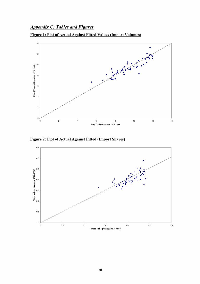
Figures 1 and 2 in Appendix C plot average values over the period 1976-1990 of

actual against fitted imports using the unscaled (open1) and scaled (open2) data

respectively. It is clear from these figures that both the average level and the average

share of trade over this period has differed widely for different countries. The figures

also suggest however that the models estimated explain the majority of the variation

in trade. If anything the plots suggest that the model using the scaled data (Figure 2)

explains less of the variation in trade. This initial view is confirmed by looking at the

correlation between the actual and the fitted values, 0.9 for the unscaled model and

0.7 for the scaled model, as well as the R2 values of the models estimated above.

In Figure 3 we plot the average values of the two openness measures for each country

against each other. An OLS regression of open1 on open2 and a constant results in a

coefficient on open2 insignificantly different from one and an insignificant constant,

suggesting that there is little difference between the two measures of openness. The R2

of this simple regression is 0.64. There are however one or two outliers that are

evident in Figure 3. The one striking outlier is Panama, which is found to have a very

high level of openness in comparison to the other countries using both measures17.

India and Brazil, the two largest countries in the sample are some distance below the

45-degree line, which indicates that they are less open using the share of imports

(open2) than with the value of imports (open1). Alternatively, two of the smaller

countries in the sample, Malawi and Malta, are some distance above the line,

suggesting that they are more open according to open2 than open1.

In Appendix C a table (Table 6) ranking the countries according to the two averaged

measures is also provided. There are some significant differences in the rankings of

countries and the correlation between the two rankings is low at 0.15. Figure 4 plots

the difference between the two openness measures for each country. The number on

the horizontal axis represents the ranking according to Open1, such that 1 refers to

Panama and so on. The two horizontal lines are one standard deviation away from

zero, with the standard deviation being that of Open1. It is clear from this figure and

Table 6 that for a number of countries, the value of openness differs a great deal 17 This result is in stark contrast to Leamer who found that although Panama was very trade dependent, her resources would suggest that she should be even more so. One possible explanation for Panama

15

depending upon the openness measure employed. Indeed, for six of the countries, the

value of openness changes by more than one standard deviation from the average

value of open118.

An interesting similarity in the measure of openness is that a number of African

countries are ranked quite high in terms of openness, contrary to conventional

wisdom. Our results suggest that once various gravity determinants and factor

endowments are controlled for, many African countries are indeed relatively open to

imports from the North, which supports the results of Rodrik (1988) and Coe and

Hoffmaister (1999). The latter finds that if anything the average African country tends

to ‘overtrade’ compared with developing countries in other regions, and suggest that

economic size, geographical distance and population can explain the low level of

trade in Africa.

3 The Role of North-South Trade on Economic Growth 3.1 Empirical Specification To test the hypothesis that openness to the North increases growth in the South we

specify a regression model with per capita GDP growth as the dependent variable.

This is estimated using panel data techniques and once again a random-effects model

is employed19. A problem arises in selecting the time interval over which to study

growth in panel studies due to the presence of cyclical effects. If annual data is used it

is necessary to model short-run dynamics. It is common to use five or ten year

averages, although this has the problem of removing much of the time series variation.

We proceed by using data on five-year averages for all of the variables, with data

being collected for 1976-1980, 1981-1985 and 1986-1990.

The model we estimate includes standard variables used in the empirical growth

literature (see for example Levine and Renelt, 1992; Durlauf and Quah, 1995)

augmented with our measure of openness. The regression model is specified as: having such a high level of openness according to our measure is that transhipments are high for Panama. 18 The six countries are Brazil, India, Mauritius, Malawi, Israel and Malta. The larger countries, such as Brazil and India, tend to be ranked higher according to open1, while the smaller countries tend to be ranked higher according to open2. This is what we expect, and indeed, this was the justification for scaling the data to begin with.

16

Avgrowmt = α + βj Ijmt + γ Openimt + εmt

Where Avgrow is the average growth in per capita GDP, α is a constant, I is a vector

of additional explanatory variables, Openi is one of our two measures of openness and

ε is an error term. Included amongst the additional variables are two time dummies

(T1 and T2) to take account of differences in growth in the different periods. A large

number of explanatory variables have been included in growth regressions and found

to be significant. The majority of these however tend not to be robust in the sense that

adding additional variables to the regression results in the original variable becoming

insignificant (see Levine and Renelt, 1992, and Sala-i-Martin, 1997).

We begin with a small number of explanatory variables, but then include additional

variables to test for robustness. Initially we include just two additional variables

alongside openness, the initial level of GDP (InitGDP) and the average investment

rate (Inv). The former is included as a catch-up term and we expect its coefficient to

be negative. Openness is considered to be one channel through which countries can

catch-up; the inclusion of this variable therefore is to account for other forms of catch-

up. The investment rate is included as a measure of the growth in the capital stock,

which we would expect to be positively related to growth20.

Another variable included is the rate of population growth (PopGrow). Ceteris

Paribus countries with high population growth would be expected to have lower per

capita growth21. We also experiment with a number of variables that proxy human

capital22. Initially we include average years of secondary schooling in the male and

female population (SyrM and SyrF respectively). We also include average number of

years of primary schooling in the male and female population (PyrM, PyrF) to

examine whether different levels of education affect growth differently. To control for

a country’s attractiveness to investment we include an index of political rights (Polrit)

19 The Hausman and Breusch-Pagan tests in general support the use of a random effects model. 20 Including the investment rate as an explanatory variable in growth regressions may be problematic since investment is likely to be endogenously determined. The results we obtain however differ very little when investment is excluded. 21 Kormendi and Meguire (1985), Levine and Renelt (1992) and Mankiw, Romer and Weil (1992) all report negative coefficients for population growth, although Levine and Renelt find the variable not to be robust. 22 Many authors include measures of human capital; examples include Barro (1991, 1998), Levine and Renelt (1992), Mankiw, Romer and Weil (1992) and Sala-i-Martin (1997).

17

and civil liberties (Civlib)23; we would expect that improvements in either of these

factors would boost growth. Many analysts control for macroeconomic conditions.

Thus we include a measure of government consumption (Gov’t) and inflation

(Inflation). Higher levels of government spending would be expected to lower growth

due to higher taxes that reduce saving and investment, and also possibly through

crowding out24. We would expect inflation to be negatively related to growth, since it

can negatively affect saving and investment (See Temple, 2000). Inflation may also to

some extent proxy for macroeconomic instability, with lower levels of inflation

reflecting greater macroeconomic stability, which would be expected to boost growth.

Dummy variables for different regions are often found significant in growth

regressions25. These are intended to capture a wide variety of political, social and

economic conditions that are specific to particular regions, but not captured by other

variables. The problem with regional dummy variables is that we don’t know what

effects they are capturing, which has led some to term such regional dummies, dumb

variables26. However, regional dummies have been included in growth regressions

elsewhere and have been found to be significant. Moreover, Temple (1999) argues

that regional dummies can be used in place of fixed effects models in empirical

growth models employing panel techniques, since much of the variation in efficiency

levels occurs between rather than within continents. Finally therefore, we include

dummy variables for Latin America (DLAT), East Asia (DEAS) and Sub-Saharan

Africa (DSSA) to see if the coefficients on openness are sensitive to their inclusion.

As mentioned above, in the empirical literature on growth few explanatory variables

are robust, in the sense that adding additional variables to a regression makes some of

the original variables insignificant. We test the robustness of the relationship between

our measure of openness and growth in a number of ways. First we use two different

measures of openness. Second we add incrementally quite a large number of variables

to examine the impact on the size and significance of existing coefficients to the

inclusion of additional variables. Third, we remove potential outliers from our sample.

23 These variables are included in the models of Barro and Lee (1994b) and Sala-i-Martin (1997). They both find that greater political rights spurs growth, but find differing effects for civil liberties. 24 See Argimon, Gonzalez Paramo and Roldan (1997) for some evidence of this. 25 Examples include Barro (1991, 1998), Barro and Lee (1994b) and Sala-i-Martin (1997). 26 Srinivasan (2000) for example argues that such variables simply quantify our ignorance.

18

This is done in two ways. Firstly, we drop the observations on Panama from our

model. Panama was found to have much higher levels of openness than any other

country in our sample27, removing this observation will allow us to examine whether

it is this observation that is driving the results obtained. Secondly, we use an

econometric technique developed by Hadi (1992, 1994) to search for potential outliers

in our growth model. The results of these tests consistently suggest that for all three

periods Kuwait is an outlier, almost certainly reflecting the fact that it is a major oil

exporter, with Nicaragua in the period 1986-90 also being an outlier. Finally,

therefore we also remove these observations to examine whether these observations

are driving any observed relationship between the measures of openness and growth.

3.2 Results The model is estimated using data on each variable for the three five-year periods for

each of the 52 Southern countries giving a total of 156 observations. In Table 3 we

report results from the growth regressions using the unscaled openness measure

(open1), while Table 4 reports the results using the scaled measure (open2) (A full list

of the variable names and their definitions are described in Table 5 in Appendix B).

If we start with the core variables most coefficients have the expected sign and the

majority are significant. The coefficient on initial GDP is negative, as expected, and

tends to be significant. The impact of investment on growth is positive and highly

significant, a result that is robust across specifications. Population growth is found to

affect growth in the manner expected, being both significant and robust across the

different specifications.

The results relating to human capital on growth are mixed28. We find that male

secondary schooling has a positive and significant impact upon growth, but that

female secondary schooling has a negative and significant impact, suggesting that

investment in female secondary education actually retards growth29. The result on the

female schooling variable is quite surprising, but not without precedent. Barro and

27 Using both openness measures and for all three periods, Panama’s openness was more than 2.7 standard deviations greater than the average value of openness. 28 When the average years of secondary schooling in the total population is included in place of the male and female secondary schooling variables, the coefficient is found to be insignificant. 29 A similar result is found by Barro and Lee (1994b).

19

Lee (1994b) amongst others have also found a negative and significant coefficient on

female schooling and argue that one explanation for this result “is that a high spread

between male and female schooling attainment is a good measure of backwardness;

hence, less female attainment signifies more backwardness and accordingly higher

growth potential through the convergence mechanism” (p. 18). Barro and Lee also

show that female schooling has beneficial impacts on infant mortality, fertility and life

expectancy.

When we include male and female average years of primary schooling, the

coefficients are the opposite to those of the secondary schooling variables. We find

that an increase in average years of primary schooling for females is positively related

to growth, while the average years of primary schooling for males is negatively

related to growth, although neither is significant. The coefficients on the average

years of secondary schooling for males and females remain unchanged when the

primary school variables are included.

The coefficients on civil liberties and political rights are not found to be significant,

(and in the case of political rights the coefficient has the wrong expected sign). The

coefficients on both government consumption and inflation have the expected sign,

but only that on the government consumption variable is significant30. Finally, the

coefficients on the regional dummy variables all have the expected sign. The

coefficients are only significant for Sub-Saharan Africa and Latin America however,

suggesting that East Asia’s relatively high growth over the period can be explained by

the variables in our model.

30 The coefficient on inflation becomes significant when the government consumption variable is removed.

20

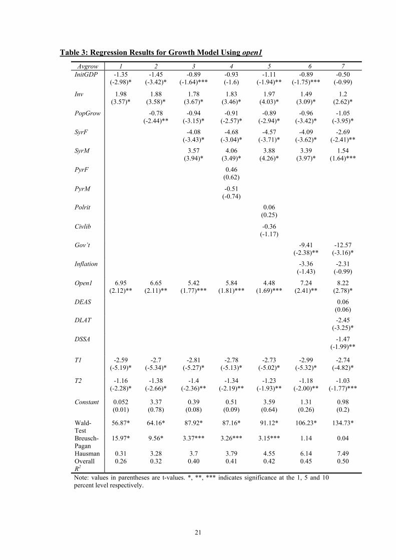
Table 3: Regression Results for Growth Model Using open1

Avgrow 1 2 3 4 5 6 7 InitGDP -1.35

(-2.98)* -1.45

(-3.42)* -0.89

(-1.64)*** -0.93 (-1.6)

-1.11 (-1.94)**

-0.89 (-1.75)***

-0.50 (-0.99)

Inv 1.98 (3.57)*

1.88 (3.58)*

1.78 (3.67)*

1.83 (3.46)*

1.97 (4.03)*

1.49 (3.09)*

1.2 (2.62)*

PopGrow -0.78 (-2.44)**

-0.94 (-3.15)*

-0.91 (-2.57)*

-0.89 (-2.94)*

-0.96 (-3.42)*

-1.05 (-3.95)*

SyrF -4.08 (-3.43)*

-4.68 (-3.04)*

-4.57 (-3.71)*

-4.09 (-3.62)*

-2.69 (-2.41)**

SyrM 3.57 (3.94)*

4.06 (3.49)*

3.88 (4.26)*

3.39 (3.97)*

1.54 (1.64)***

PyrF 0.46 (0.62)

PyrM -0.51 (-0.74)

Polrit 0.06 (0.25)

Civlib -0.36 (-1.17)

Gov’t -9.41 (-2.38)**

-12.57 (-3.16)*

Inflation -3.36 (-1.43)

-2.31 (-0.99)

Open1 6.95 (2.12)**

6.65 (2.11)**

5.42 (1.77)***

5.84 (1.81)***

4.48 (1.69)***

7.24 (2.41)**

8.22 (2.78)*

DEAS 0.06 (0.06)

DLAT -2.45 (-3.25)*

DSSA -1.47 (-1.99)**

T1 -2.59 (-5.19)*

-2.7 (-5.34)*

-2.81 (-5.27)*

-2.78 (-5.13)*

-2.73 (-5.02)*

-2.99 (-5.32)*

-2.74 (-4.82)*

T2 -1.16 (-2.28)*

-1.38 (-2.66)*

-1.4 (-2.36)**

-1.34 (-2.19)**

-1.23 (-1.93)**

-1.18 (-2.00)**

-1.03 (-1.77)***

Constant 0.052 (0.01)

3.37 (0.78)

0.39 (0.08)

0.51 (0.09)

3.59 (0.64)

1.31 (0.26)

0.98 (0.2)

Wald-Test

56.87* 64.16* 87.92* 87.16* 91.12* 106.23* 134.73*

Breusch-Pagan

15.97* 9.56* 3.37*** 3.26*** 3.15*** 1.14 0.04

Hausman 0.31 3.28 3.7 3.79 4.55 6.14 7.49 Overall R2

0.26 0.32 0.40 0.41 0.42 0.45 0.50

Note: values in parentheses are t-values. *, **, *** indicates significance at the 1, 5 and 10 percent level respectively.

21

Table 4: Regression Results for Growth Model Using open2

Avgrow 1 2 3 4 5 6 7 InitGPP -1.41

(-3.09)* -1.50

(-3.49)* -0.86

(-1.59) -0.88

(-1.49) -1.14

(-2.01)** -0.86

(-1.70)*** -0.51

(-1.04)

Inv 2.15 (3.9)*

2.05 (3.91)*

1.92 (3.97)*

2.03 (3.77)*

1.85 (3.77)*

1.63 (3.48)*

1.33 (2.95)*

PopGrow -0.75 (-2.33)**

-0.93 (-3.11)*

-0.93 (-2.62)*

-0.90 (-2.97)*

-0.94 (-3.41)*

-1.01 (-3.87)*

SyrF -4.4 (-3.63)*

-5.09 (-3.25)*

-4.3 (-3.56)*

-4.57 (-4.01)*

-3.23 (-2.89)*

SyrM 3.75 (4.18)*

4.31 (3.73)*

3.72 (4.04)*

3.62 (4.34)*

1.81 (1.99)**

PyrF 0.48 (0.64)

PyrM -0.59 (-0.86)

Polrit 0.07 (0.27)

Civlib -0.39 (-1.27)

Gov’t -10.63 (-2.67)*

-13.47 (-3.41)*

Inflation -3.23 (-1.38)

-2.22 (-0.56)

Open2 5.39 (1.92)***

4.82 (1.79)***

4.96 (1.91)***

5.66 (2.01)**

5.19 (1.68)***

7.13 (2.78)*

7.7 (3.19)*

DEAS 0.06 (0.07)

DLAT -2.39 (-3.27)*

DSSA -1.71 (-2.36)**

T1 -2.58 (-5.18)*

-2.7 (-5.33)*

-2.77 (-5.18)*

-2.71 (-4.96)*

-2.75 (-5.08)*

-2.91 (-5.14)*

-2.66 (-4.68)*

T2 -1.14 (-2.25)**

-1.37 (-2.62)*

-1.32 (-2.2)**

-1.22 (-1.94)**

-1.27 (-2.02)**

-1.05 (-1.76)***

-0.90 (-1.53)

Constant 1.63 (0.41)

5.09 (1.26)

0.24 (0.05)

-0.06 (-0.01)

3.6 (0.64)

0.93 (0.19)

1.33 (0.29)

Wald-Test

55.89* 62.35* 88.68* 88.4* 91.17* 110.33 141.28*

Breusch-Pagan

16.39* 9.94* 3.38* 3.22* 3.16* 0.87 0.14

Hausman 0.67 3.95 3.97 3.85 4.64 6.48 7.75 Overall R2

0.26 0.31 0.41 0.41 0.42 0.46 0.51

Note: values in parentheses are t-values. *, **, *** indicates significance at the 1, 5 and 10 percent level respectively.

22

Turning now to openness we see that for both measures the coefficient is positive and

large, suggesting that growth is positively related to openness to imports from the

North. Furthermore, the coefficients are all significant at least at the 10 percent level,

and once regional factors have been taken account of, the coefficients are significant

at the 1 percent level. The value of the coefficient however is variable, falling when

the various measures of human capital are included. The coefficient on open1 tends to

be higher than that on the scaled measure of openness, open2. The results suggest that

an increase in openness by one standard deviation would increase growth by between

0.39 and 0.72 percent using open1 as our openness measure and between 0.51 and

0.82 percent using open2 as our measure of openness.

The results suggest that whichever of the two openness measures is used, a positive

and significant relationship between openness and growth is found, suggesting that

our measure of openness is quite robust. Moreover, the inclusion of a large number of

additional variables into our model doesn’t alter the sign or significance of the

openness measure. The value of the coefficient does change to some extent,

particularly when human capital is included, but the relationship between openness

and growth is always significant.

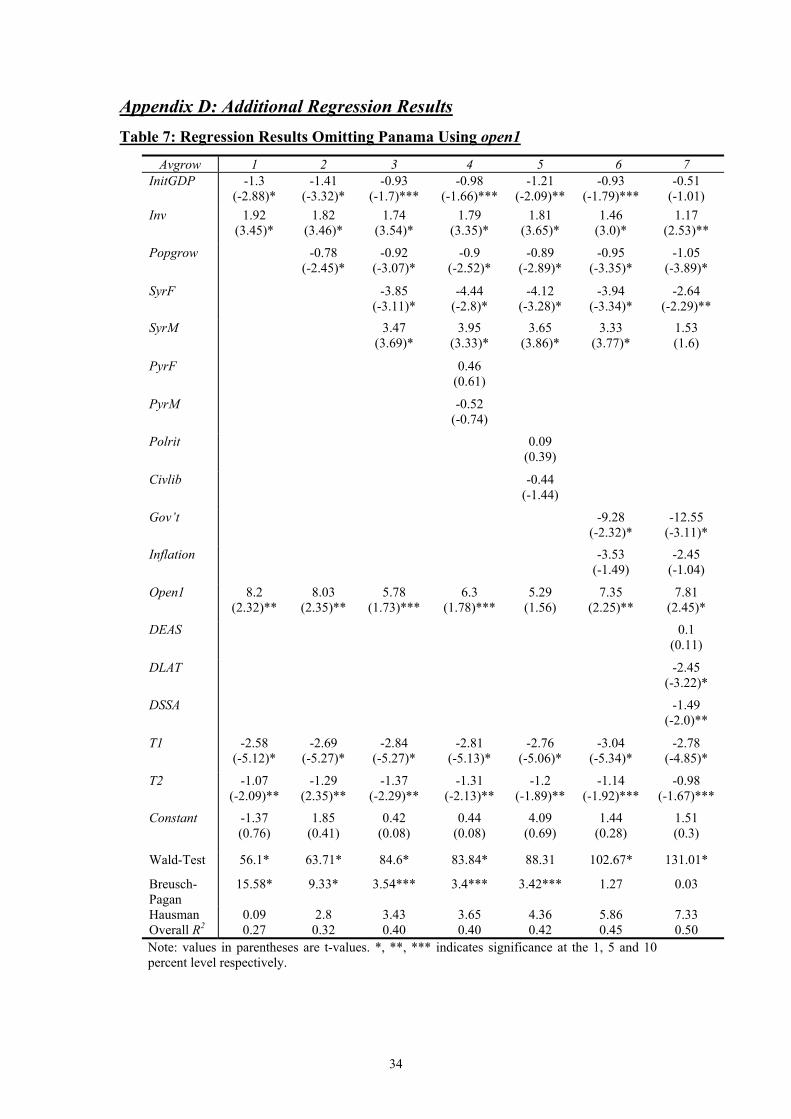
The results of removing the various outliers in the sample are reported in tables 7 to

10 in Appendix D. When removed the one striking outlier according to the measure of

openness, Panama, has very little effect on the initial variables in the growth model,

although initial GDP becomes insignificant in a number of cases (See Tables 7 and 8).

More importantly, the coefficients on the openness measures are still positive and

often increase in size. In one case the coefficient on our measure of openness is

insignificant, but it is often the case that the coefficients have a higher level of

significance after removing Panama. Tables 9 and 10 report the results after removing

all three observations on Kuwait and the final observation on Nicaragua. The results

are broadly similar to those found for the full sample of countries, with both measures

of openness always being positive and significant.

23

4 Conclusions For a long time it has been suggested that openness to international trade can have a

positive impact on growth. The theory that relates openness to growth however is not

conclusive on this hypothesis, openness can be shown to increase or reduce growth

depending upon the country in question and upon the goods in which the country

specialises in following trade liberalisation.

We examine one particular form of trade, namely North-South trade, and its impact on

economic growth. Such a focus is justified by the endogenous growth theories, which

suggest that countries benefit from trade through the importation of capital and

intermediate goods, and technology. We began by constructing a measure of openness

based on the deviation of actual from predicted imports from the North. We modelled

imports as being determined by the factor endowments of the importer and by various

gravity determinants. The model developed explained well the cross-country variation

in the level of imports of the South.

Using this measure we estimated the impact of openness to goods from the North on

economic growth. We showed that openness was significantly related to growth, with

the positive impact being quite large. We were also able to show that this relationship

was robust in the sense that the coefficient was always positive and significant. This

was true regardless of the openness measure employed, the additional variables

included in the model and the removal of influential outliers. The coefficient on

openness did vary however, depending upon the measure used and the variables

included in the model.

One important caveat of the measure of openness developed is that it is based on the

deviation of actual trade from that expected given a country’s factor endowments and

geographical characteristics. While this may be a good indicator of government trade

restrictions, it may also be measuring other trade limiting forces, such as poor internal

infrastructure31. An implication of these results then is that lowering impediments to

imports from the North can be helpful to growth. One such impediment is trade

restrictions, but the removal or reduction of these may not be sufficient to enhance

24

growth. Other impediments not captured in the empirical model may also be

important. If imports from the North are low because of poor internal infrastructure

for example, reducing trade restrictions may not improve growth. In this case,

governments should also look to improve the level of infrastructure within the

economy, which can enhance imports by reducing internal transport costs.

31 A lack of data on measures of internal infrastructure for our sample of countries precluded us from including a variable capturing this in our model of imports.

25

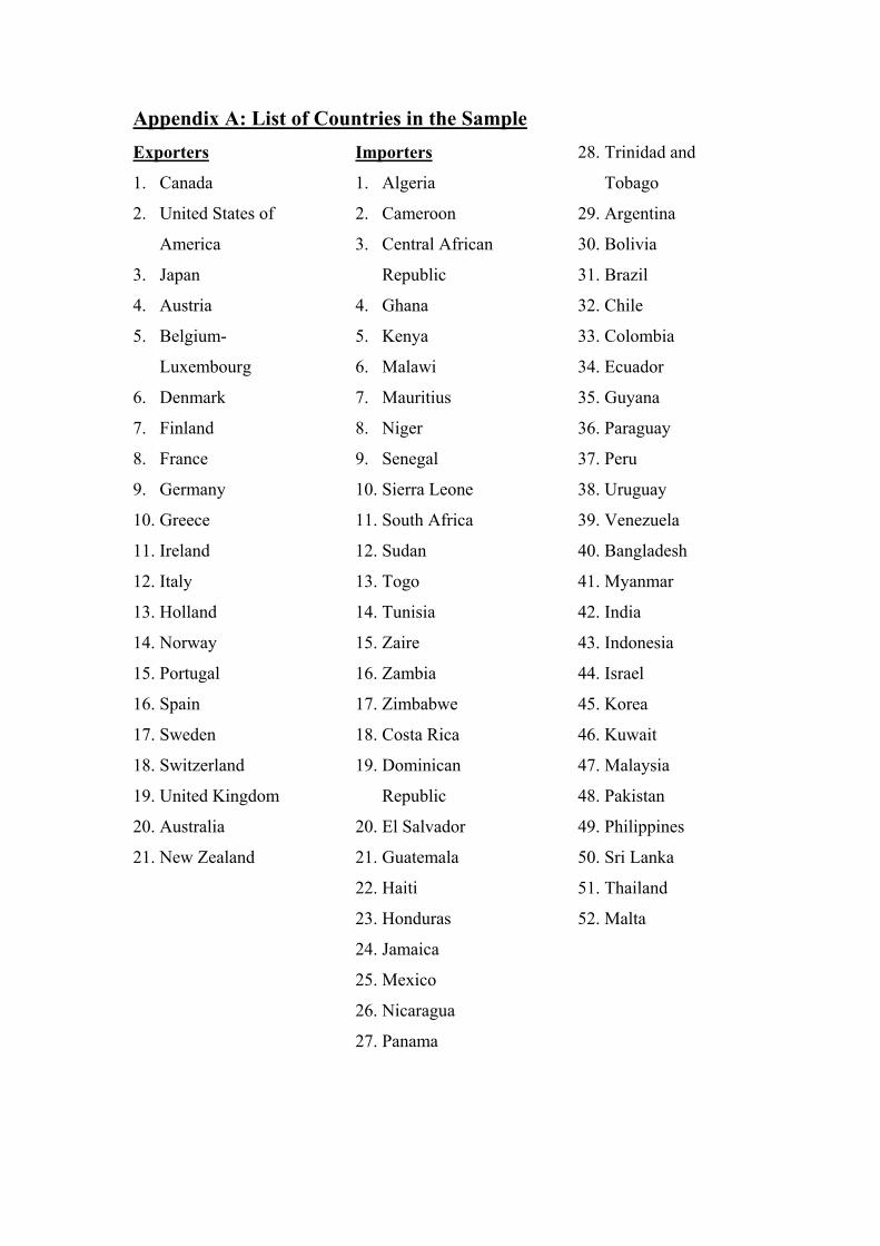
Appendix A: List of Countries in the Sample Exporters

1. Canada

2. United States of

America

3. Japan

4. Austria

5. Belgium-

Luxembourg

6. Denmark

7. Finland

8. France

9. Germany

10. Greece

11. Ireland

12. Italy

13. Holland

14. Norway

15. Portugal

16. Spain

17. Sweden

18. Switzerland

19. United Kingdom

20. Australia

21. New Zealand

Importers

1. Algeria

2. Cameroon

3. Central African

Republic

4. Ghana

5. Kenya

6. Malawi

7. Mauritius

8. Niger

9. Senegal

10. Sierra Leone

11. South Africa

12. Sudan

13. Togo

14. Tunisia

15. Zaire

16. Zambia

17. Zimbabwe

18. Costa Rica

19. Dominican

Republic

20. El Salvador

21. Guatemala

22. Haiti

23. Honduras

24. Jamaica

25. Mexico

26. Nicaragua

27. Panama

28. Trinidad and

Tobago

29. Argentina

30. Bolivia

31. Brazil

32. Chile

33. Colombia

34. Ecuador

35. Guyana

36. Paraguay

37. Peru

38. Uruguay

39. Venezuela

40. Bangladesh

41. Myanmar

42. India

43. Indonesia

44. Israel

45. Korea

46. Kuwait

47. Malaysia

48. Pakistan

49. Philippines

50. Sri Lanka

51. Thailand

52. Malta

Appendix B: Data Sources, Construction and Variable Names Much of the data used in this paper was taken from the Summers and Heston (1991)

database (SH) and the Barro and Lee datasets (1994a, 2000). Data on GDP, growth

rates, population, human capital, government consumption, inflation and the terms of

trade were all taken from these sources. Data on the labour force and investment were

taken from the dataset constructed by Greenaway, Morgan and Wright (1997),

denoted as GMW in the table below. Data on distance, common languages and

common borders were taken from a web-site maintained by Jon Haveman. Data on

area was taken either from the Barro and Lee dataset (1994a) or from the Central

Intelligence Agency (CIA) World Factbook (1998). Data on total manufacturing

imports from the Northern countries are measured as exports from the Northern

country to the Southern country and were taken from the publication International

Trade by Commodities Statistics, 1961-1990. Exports of primary products were taken

from The World Bank Indicators database (1994). A full list of the variables along

with a brief description of each is provided in the table below.

27

Table 5: Variable Names, Description and Sources Variable Name Description Construction Source

Area Total area of importer in square miles (in logs)

Barro and Lee 1994a, CIA World Factbook

Avgrow Annual growth of per capita GDP

SH

Capital The value of the capital stock in the importing country (in

logs)

Constructed using investment data and assuming a 15-year

average life of assets

GMW

Civlib Measure of civil liberties Index taking a value between 1 and 7 (1 greatest civil

liberties)

Barro and Lee 1994a

Comlang Dummy variable taking the value 1 if the importer and exporter share a common

language

Haveman

DEAS Dummy variable taking value 1 if the country is in East Asia

Barro and Lee 1994a

DLAT Dummy variable taking value 1 if the country is in Latin

America

Barro and Lee 1994a

DSSA Dummy variable taking value 1 if the country is in Sub-

Saharan Africa

Barro and Lee 1994a

Dist The Logged distance between the importer and exporter in

square

Great circle distance between capital cities in miles

Haveman

DTTI Terms of trade of the importing country

Barro and Lee 1994a

GDPIN The logged real value of GDPs of the importer and exporter

interacted

GDP of importer multiplied by the GDP of the exporter

SH

GDPPC The logged real value of the GDP per capita of the importer

and exporter interacted

Per capita GDP of importer multiplied by the GDP per

capita of the exporter

SH

Gov’t Real Government share of GDP (%) in 1985 international

prices

SH

InitGDP Level of GDP in 1976 in constant dollars

SH

Inflation Average rate of inflation Constructed using price level data

SH

Inv Annual Investment in constant Dollars

GMW

K/Worker The value of capital per worker (in logs)

Capital divided by the Labour Own calculations

Labour The (logged) number in the workforce of the importing

country

GMW

Land/Worker The ratio of land to the labour force

Area divided by Labour Own calculations

28

LockM Dummy variable taking the value 1 if the importer is

landlocked

Haveman

LockX Dummy variable taking the value 1 if the exporter is

landlocked

Haveman

LogTrade The (logged) real value of total manufacturing imports from each Northern country

International Trade by Commodities Statistics,

1961-1990, (OECD)

Polrit Measure of political rights Index taking a value between 1 and 7 (1 greatest political

rights)

Barro and Lee 1994a

PopGrow Annual rate of population growth

Barro and Lee 1994a

PriX The logged real value of primary exports of the

importing country

Current value of exports deflated by GDP deflator

World Bank Indicators Database

PriX/GDP The share of primary exports in GDP

PriX divided by GDP of the importing country

Own calculations

PyrF Average years of primary schooling in the female

population

Barro and Lee 2000

PyrM Average years of primary schooling in the male

population

Barro and Lee 2000

Skilled Proxy for the stock of human capital in the importing

country (in logs)

Percentage of people over 25 with higher education multiplied by Labour

Barro and Lee 1994a, GMW

Skill/Unskill The ratio of skilled to unskilled workers

Skilled divided by Unskilled Own calculations

SyrF Average years of secondary schooling in the female

population

Barro and Lee 2000

SyrM Average years of secondary schooling in the male

population

Barro and Lee 2000

TradeShare The share of imports from each Northern country in GDP

Real value of imports divided by GDP of importer

OECD and SH

Unskilled Proxy for unskilled labour (logged value)

Labour less Skilled Own calculations

29

Appendix C: Tables and Figures Figure 1: Plot of Actual Against Fitted Values (Import Volumes)

0

2

4

6

8

10

12

14

0 2 4 6 8 10 12

Log Trade (Average 1976-1990)

Fitte

d Va

lues

(Ave

rage

197

6-19

90)

14

Figure 2: Plot of Actual Against Fitted (Import Shares)

0

0.1

0.2

0.3

0.4

0.5

0.6

0.7

0 0.1 0.2 0.3 0.4 0.5 0.6

Trade Ratio (Average 1976-1990)

Fitte

d Va

lues

(Ave

rage

197

6-19

90)

30

Figure 3: Plot of open1 Against open2

0

0.2

0.4

0.6

0.8

1

1.2

1.4

0 0.2 0.4 0.6 0.8 1 1.2 1.4

Open1 (Average 1976-1990)

Ope

n2 (A

vera

ge 1

976-

1990

)

31

Table 6: Ranking of Countries by Openness Measure

Rank open1 open2 1 Panama Panama 2 Philippines Malawi 3 Pakistan Israel 4 Zambia Malta 5 Thailand Philippines 6 Bolivia Zambia 7 Peru Sierra Leone 8 Korea Mauritius 9 Chile Sri Lanka

10 Malawi Ecuador 11 Bangladesh Costa Rica 12 Paraguay Dominican Republic 13 Israel Uruguay 14 Sri Lanka Chile 15 Uruguay Korea 16 Kenya Peru 17 Ecuador Haiti 18 India Togo 19 Malta Pakistan 20 Sierra Leone Kenya 21 Venezuela Bangladesh 22 Malaysia Thailand 23 Dominican Republic Jamaica 24 South Africa Paraguay 25 Indonesia El Salvador 26 Costa Rica Malaysia 27 Zaire Bolivia 28 Mexico Kuwait 29 Colombia Venezuela 30 Brazil Guatemala 31 Togo Nicaragua 32 Argentina Indonesia 33 El Salvador Honduras 34 Haiti Zaire 35 Jamaica Trinidad and Tobago 36 Tunisia South Africa 37 Mauritius Senegal 38 Nicaragua Tunisia 39 Guyana Colombia 40 Senegal Ghana 41 Sudan Guyana 42 Guatemala Mexico 43 Kuwait Cameroon 44 Honduras Argentina 45 Ghana India 46 Cameroon Sudan 47 Myanmar Brazil 48 Trinidad and Tobago Niger 49 Algeria Myanmar 50 Niger Zimbabwe 51 Zimbabwe Algeria 52 Central African Republic Central African Republic

32

Figure 4.4: Difference in Openness between open1 and open2

-0,15

-0,1

-0,05

0

0,05

0,1

0,15

1 2 3 4 5 6 7 8 9 10 11 12 13 14 15 16 17 18 19 20 21 22 23 24 25 26 27 28 29 30 31 32 33 34 35 36 37 38 39 40 41 42 43 44 45 46 47 48 49 50 51 52

R an k

Chan

ge in

Ope

nnes

s

33

Appendix D: Additional Regression Results Table 7: Regression Results Omitting Panama Using open1

Avgrow 1 2 3 4 5 6 7 InitGDP -1.3

(-2.88)* -1.41

(-3.32)* -0.93

(-1.7)*** -0.98

(-1.66)*** -1.21

(-2.09)** -0.93

(-1.79)*** -0.51

(-1.01) Inv 1.92

(3.45)* 1.82

(3.46)* 1.74

(3.54)* 1.79

(3.35)* 1.81

(3.65)* 1.46

(3.0)* 1.17

(2.53)**

Popgrow -0.78 (-2.45)*

-0.92 (-3.07)*

-0.9 (-2.52)*

-0.89 (-2.89)*

-0.95 (-3.35)*

-1.05 (-3.89)*

SyrF -3.85 (-3.11)*

-4.44 (-2.8)*

-4.12 (-3.28)*

-3.94 (-3.34)*

-2.64 (-2.29)**

SyrM 3.47 (3.69)*

3.95 (3.33)*

3.65 (3.86)*

3.33 (3.77)*

1.53 (1.6)

PyrF 0.46 (0.61)

PyrM -0.52 (-0.74)

Polrit 0.09 (0.39)

Civlib -0.44 (-1.44)

Gov’t -9.28 (-2.32)*

-12.55 (-3.11)*

Inflation -3.53 (-1.49)

-2.45 (-1.04)

Open1 8.2 (2.32)**

8.03 (2.35)**

5.78 (1.73)***

6.3 (1.78)***

5.29 (1.56)

7.35 (2.25)**

7.81 (2.45)*

DEAS 0.1 (0.11)

DLAT -2.45 (-3.22)*

DSSA -1.49 (-2.0)**

T1 -2.58 (-5.12)*

-2.69 (-5.27)*

-2.84 (-5.27)*

-2.81 (-5.13)*

-2.76 (-5.06)*

-3.04 (-5.34)*

-2.78 (-4.85)*

T2 -1.07 (-2.09)**

-1.29 (2.35)**

-1.37 (-2.29)**

-1.31 (-2.13)**

-1.2 (-1.89)**

-1.14 (-1.92)***

-0.98 (-1.67)***

Constant -1.37 (0.76)

1.85 (0.41)

0.42 (0.08)

0.44 (0.08)

4.09 (0.69)

1.44 (0.28)

1.51 (0.3)

Wald-Test 56.1* 63.71* 84.6* 83.84* 88.31 102.67* 131.01*

Breusch-Pagan

15.58* 9.33* 3.54*** 3.4*** 3.42*** 1.27 0.03

Hausman 0.09 2.8 3.43 3.65 4.36 5.86 7.33 Overall R2 0.27 0.32 0.40 0.40 0.42 0.45 0.50 Note: values in parentheses are t-values. *, **, *** indicates significance at the 1, 5 and 10 percent level respectively.

34

Table 8: Regression Results Omitting Panama Using open2

Avgrow 1 2 3 4 5 6 7 InitGDP -1.38

(-3.01)* -1.47

(-3.41)* -0.9

(-1.65)*** -0.92

(-1.54) -1.17

(-2.02)** -0.89

(-1.74)*** -0.52

(-1.04)

Inv 2.1 (3.81)*

2.01 (3.82)*

1.89 (3.85)*

2.01 (3.68)*

1.94 (3.91)*

1.61 (3.38)*

1.29 (2.84)*

Popgrow -0.75 (-2.31)**

-0.91 (-3.03)*

-0.92 (-2.57)*

-0.88 (-2.86)*

-0.93 (-3.33)*

-1.01 (-3.81)*

SyrF -4.19 (-3.35)*

-4.86 (-3.05)*

-4.39 (-3.47)*

-4.41 (-3.74)*

-3.16 (-2.76)*

SyrM 3.65 (3.97)*

4.21 (3.59)*

3.82 (4.09)*

3.55 (4.15)*

1.78 (1.93)***

PyrF 0.48 (0.63)

PyrM -0.62 (-0.87)

Polrit 0.09 (0.36)

Civlib -0.41 (-1.34)

Gov’t -10.52 (-2.61)*

-13.48 (-3.37)*

Inflation -3.4 (-1.44)

-2.36 (-1.01)

Open2 6.63 (2.18)**

6.05 (2.07)**

5.34 (1.89)***

6.19 (2.02)**

4.61 (1.6)

7.33 (2.67)*

7.49 (2.91)*

DEAS 0.1 (0.11)

DLAT -2.41 (-3.24)*

DSSA -1.72 (-2.65)**

T1 -2.57 (-5.09)*

-2.68 (-5.25)*

-2.79 (-5.18)*

-2.73 (-4.95)*

-2.73 (-5.0)*

-2.95 (-5.16)*

-2.69 (-4.7)*

T2 -1.04 (-2.03)**

-1.26 (-2.39)**

-1.29 (-2.12)**

-1.17 (-1.86)***

-1.15 (-1.79)***

-1.0 (-1.67)***

-0.84 (-1.43)

Constant 0.28 (0.07)

3.72 (0.88)

0.23 (0.04)

-0.24 (-0.04)

4.04 (0.69)

0.97 (0.19)

1.67 (0.36)

Wald-Test 55.36* 61.84* 85.47* 85.27* 88.44* 106.87* 137.61

Breusch-Pagan

16.41* 10.1* 3.57*** 3.39*** 3.44*** 1.0 0.11

Hausman 0.26 3.33 3.78 3.75 4.57 6.25 7.66 Overall R2 0.26 0.31 0.40 0.52 0.42 0.46 0.51 Note: values in parentheses are t-values. *, **, *** indicates significance at the 1, 5 and 10 percent level respectively.

35

Table 9: Regression Results Using open1 and Omitting Outliers

Avgrow 1 2 3 4 5 6 7 InitGDP -1.05

(-2.15)** -1.47

(-2.91)* -0.92

(-1.62) -0.79

(-1.25) -1.12

(-1.87)*** -1.04

(-1.91)*** -0.4

(-0.78)

Inv 2.0 (3.7)*

1.97 (3.77)*

1.82 (3.72)*

1.98 (3.77)*

1.91 (3.86)*

1.52 (3.1)*

1.09 (2.39)**

Popgrow -0.85 (-2.22)**

-0.91 (-2.4)**

-0.92 (-2.34)**

-0.94 (-2.47)**

-1.03 (-2.8)*

-0.81 (-2.35)**

SyrF -3.72 (-2.98)*

-3.97 (-2.3)**

-4.08 (-3.17)*

-3.78 (-3.14)*

-1.82 (-1.53)

SyrM 3.38 (3.67)*

3.81 (3.23)*

3.54 (3.76)*

3.26 (3.68)*

1.27 (1.36)

PyrF 0.24 (0.31)

PyrM -0.54 (-0.78)

Polrit 0.13 (0.53)

Civlib -0.40 (-1.31)

Gov’t -9.22 (-2.26)**

-12.36 (-3.12)*

Inflation -2.64 (-0.75)

-1.24 (-0.35)

Open1 6.88 (2.13)**

7.14 (2.27)**

5.56 (1.77)***

6.27 (1.94)***

5.64 (1.78)***

7.31 (2.31)**

7.1 (2.36)**

DEAS -0.07 (-0.08)

DLAT -2.91 (-3.69)*

DSSA -1.72 (-2.29)**

T1 -2.46 (-4.98)*

-2.54 (-5.11)*

-2.68 (-5.04)*

-2.61 (-4.85)*

-2.58 (-4.76)*

-2.83 (-4.58)*

-2.61 (-4.22)*

T2 -0.92 (-1.8)***

-1.12 (-2.17)**

-1.23 (-2.05)**

-1.11 (-1.82)***

-1.04 (-1.64)***

-1.15 (-1.92)***

-1.09 (-1.86)***

Constant -2.15 (-0.5)

2.87 (0.61)

0.21 (0.04)

-1.05 (0.86)

2.63 (0.54)

2.22 (0.43)

1.05 (0.22)

Wald-Test 53.56* 59.28* 77.52* 77.9* 79.7* 87.28* 119.1*

Breusch-Pagan

14.27* 10.44* 3.64*** 3.46*** 3.49*** 1.46 0.09

Hausman 2.22 2.72 3.87 4.14 0.84 6.17 8.27 Overall R2 0.25 0.29 0.37 0.38 0.38 0.41 0.47

Note: values in parentheses are t-values. *, **, *** indicates significance at the 1, 5 and 10 percent level respectively.

36

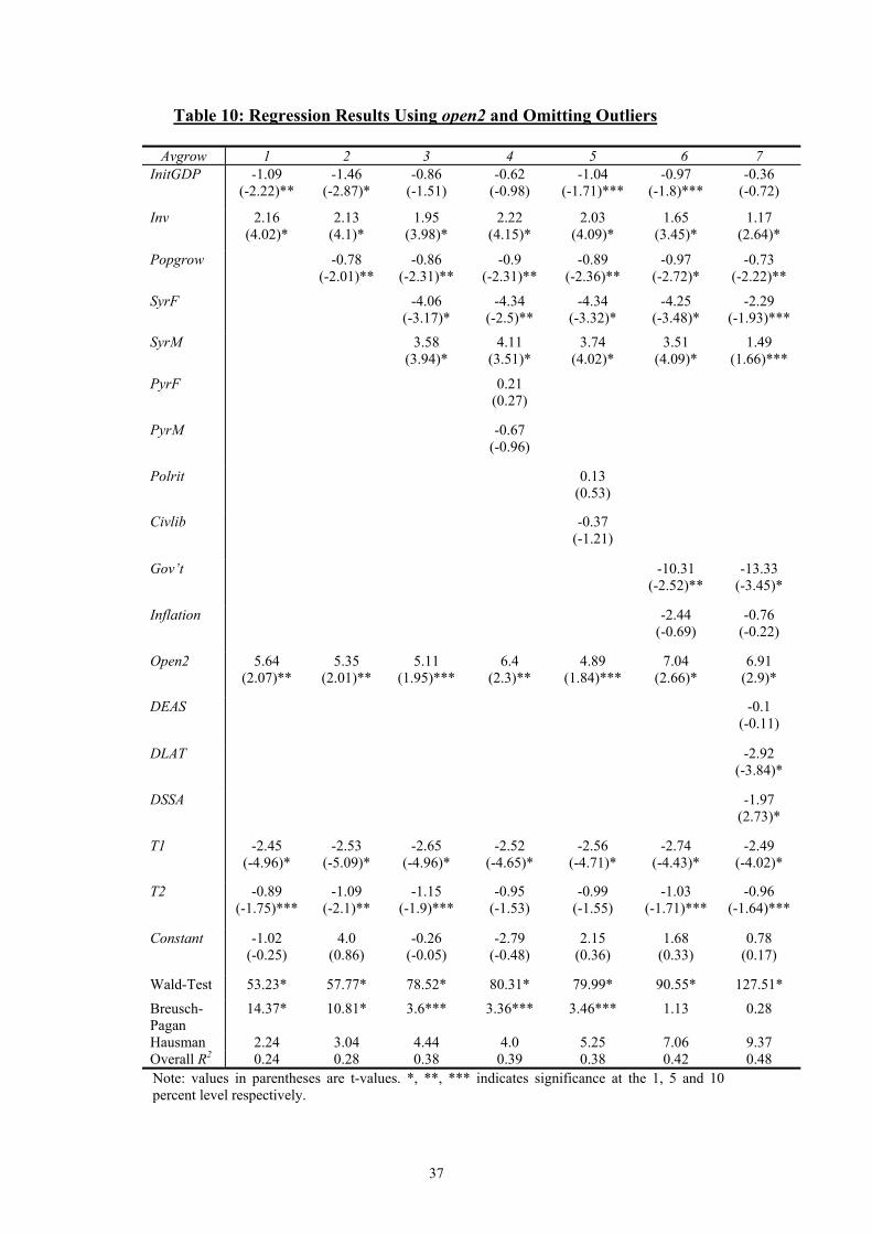
Table 10: Regression Results Using open2 and Omitting Outliers

Avgrow 1 2 3 4 5 6 7 InitGDP -1.09

(-2.22)** -1.46

(-2.87)* -0.86

(-1.51) -0.62

(-0.98) -1.04

(-1.71)*** -0.97

(-1.8)*** -0.36

(-0.72)

Inv 2.16 (4.02)*

2.13 (4.1)*

1.95 (3.98)*

2.22 (4.15)*

2.03 (4.09)*

1.65 (3.45)*

1.17 (2.64)*

Popgrow -0.78 (-2.01)**

-0.86 (-2.31)**

-0.9 (-2.31)**

-0.89 (-2.36)**

-0.97 (-2.72)*

-0.73 (-2.22)**

SyrF -4.06 (-3.17)*

-4.34 (-2.5)**

-4.34 (-3.32)*

-4.25 (-3.48)*

-2.29 (-1.93)***

SyrM 3.58 (3.94)*

4.11 (3.51)*

3.74 (4.02)*

3.51 (4.09)*

1.49 (1.66)***

PyrF 0.21 (0.27)

PyrM -0.67 (-0.96)

Polrit 0.13 (0.53)

Civlib -0.37 (-1.21)

Gov’t -10.31 (-2.52)**

-13.33 (-3.45)*

Inflation -2.44 (-0.69)

-0.76 (-0.22)

Open2 5.64 (2.07)**

5.35 (2.01)**

5.11 (1.95)***

6.4 (2.3)**

4.89 (1.84)***

7.04 (2.66)*

6.91 (2.9)*

DEAS -0.1 (-0.11)

DLAT -2.92 (-3.84)*

DSSA -1.97 (2.73)*

T1 -2.45 (-4.96)*

-2.53 (-5.09)*

-2.65 (-4.96)*

-2.52 (-4.65)*

-2.56 (-4.71)*

-2.74 (-4.43)*

-2.49 (-4.02)*

T2 -0.89 (-1.75)***

-1.09 (-2.1)**

-1.15 (-1.9)***

-0.95 (-1.53)

-0.99 (-1.55)

-1.03 (-1.71)***

-0.96 (-1.64)***

Constant -1.02 (-0.25)

4.0 (0.86)

-0.26 (-0.05)

-2.79 (-0.48)

2.15 (0.36)

1.68 (0.33)

0.78 (0.17)

Wald-Test 53.23* 57.77* 78.52* 80.31* 79.99* 90.55* 127.51*

Breusch-Pagan

14.37* 10.81* 3.6*** 3.36*** 3.46*** 1.13 0.28

Hausman 2.24 3.04 4.44 4.0 5.25 7.06 9.37 Overall R2 0.24 0.28 0.38 0.39 0.38 0.42 0.48 Note: values in parentheses are t-values. *, **, *** indicates significance at the 1, 5 and 10 percent level respectively.

37

References Anderson, James E. (1979). “A Theoretical Foundation for the Gravity Equation,”

American Economic Review, 69, 106-116. Argimon, I., Gonzalez Paramo, J. M. and J. M. Roldan (1997). “Evidence of Public

Spending Crowding-Out from a Panel of OECD Countries,” Applied Economics, 29, 1001-1010.

Barro, Robert J (1991). “Economic Growth in a Cross-Section of Countries,”

Quarterly Journal of Economics, 106, 407-443. Barro, Robert J. (1998). Determinants of Economic Growth, Cambridge MA, MIT

Press. Barro, Robert J. and Jong-Wha Lee (1994a). Dataset for a Panel of 138 Countries,

Harvard University. Barro, Robert J. and Jong-Wha Lee (1994b). “Sources of Economic Growth,”

Carnegie Rochester Conference Series on Public Policy, 40, 1-46. Barro, Robert J. and Jong-Wha Lee (2000). “International Data on Educational

Attainment: Updates and Implications,” Working Paper no. 42, Center for International Development, Harvard University.

Bayoumi, Tamin and Barry Eichengreen (1995). “Is Regionalism Simply a Diversion?

Evidence from the Evolution of the EC and EFTA,” CEPR Discussion Paper no. 1294, London, CEPR.

Bergstrand, Jeffrey H. (1985). “The Gravity Equation in International Trade: Some

Microeconomic Foundations and Empirical Evidence,” The Economic Journal, 67, 474-481.

Bougheas, Spiros, Panicos O. Demetriades and Edgar L.W. Morgenroth (1999).

“Infrastructure, Transport Costs and Trade,” Journal of International Economics, 47, 169-189.

Central Intelligence Agency (1998). CIA World Factbook 1998, Washington, DC,

Central Intelligence Agency. Chenery, Hollis B. and Moshe Syrquin (1975). Patterns of Development, 1950-1970,

New York, Oxford University Press. Chenery, Hollis B. and Moshe Syrquin (1989). “Three Decades of Industrialisation,”

World Bank Economic Review, 3, 145-181. Coe, David T. and Elhanan Helpman (1995). “International R&D Spillovers,”

European Economic Review, 39, 859-887.

38

Coe, David T., Elhanan Helpman and Alexander W. Hoffmaister (1997). “North-South R&D Spillovers,” The Economic Journal, 107, 139-149.

Coe, David T. and Alexander W. Hoffmaister (1998). “North-South Trade: Is Africa

Unusual?” Working Paper of the International Monetary Fund. Dollar, David (1992). “Outward-Oriented Developing Economies Do Grow More

Rapidly: Evidence from 95 LDCs, 1976-1985,” Economic Development and Cultural Change, 40, 523-544.

Durlauf, Steven N. and Danny T. Quah (1995). “The New Empirics of Economic

Growth,” Centre for Economic Performance Discussion Paper no. 384. Frankel, J. A. (1997). Regional Trading Blocs in the World Economic System,

Washington, DC, Institute for International Economics. Greenaway, David, Wyn Morgan and Peter Wright (1997). “Trade Liberalisation and

Growth in Developing Countries: Some New Evidence,” World Development, 25, 1885-1892.

Greene, William H. (1981). “On the Asymptotic Bias of the Ordinary Least Squares

Estimator of the Tobit Model,” Econometrica, 49, 505-513. Grossman, Gene M., and Elhanan Helpman (1991). Innovation and Growth in the

Global Economy, Cambridge, MA, MIT Press. Hadi, Ali S. (1992). “Identifying Multiple Outliers in Multivariate Data,” Journal of

the Royal Statistical Society, Series B (Methodological), 54, 761-771. Hadi, Ali S. (1994). “A Modification of a Method for the Identification of Outliers in

Multivariate Samples,” Journal of the Royal Statistical Society, Series B (Methodological), 56, 393-396.

Harrison, Ann (1996). “Openness and Growth: A Time-Series, Cross-Country

Analysis for Developing Countries,” Journal of Development Economics, 48, 419-447.

Helliwell, John F. (1998). How Much do Natural Borders Matter?, Washington, DC,

Brookings Institute. Helpman, Elhanan and Paul Krugman (1985). Market Structure and Foreign Trade,

Cambridge, MA, MIT Press. Kleiman, Ephraim (1976). “Trade and the Decline of Colonialism,” Economic

Journal, 86, 459-480. Kormendi, Roger and P. Mequire (1985). “Macroeconomic Determinants of Growth:

Cross-Country Evidence,” Journal of Monetary Economics, 16, 141-163.

39

Leamer, Edward (1974). “The commodity composition of international trade in manufactures: an empirical analysis,” Oxford Economic Papers, 26(3), 350-374.

Leamer, Edward (1984). Sources of International Comparative Advantage,

Cambridge, MA, MIT Press. Leamer, Edward (1988). “Measures of Openness,” in Robert Baldwin, ed., Trade

Policy Issues and Empirical Analysis, Chicago, IL, University of Chicago Press.

Lee, Jong-Wha (1993). “International Trade, Distortions and Long-Run Economic

Growth,” IMF Staff Papers, Washington, DC, IMF. Lee, Jong-Wha (1995). “Capital Goods Imports and Long-Run Growth,” Journal of

Development Economics, 48, 91-110. Levine, Ross, and David Renelt (1992). “A Sensitivity Analysis of Cross-Country

Growth Regressions,” American Economic Review, 82, 942-963. Limao, N. and Anthony Venables (1999). “Infrastructure, Geographical Disadvantage

and Transport Costs,” Mimeo. Mankiw, N. Gregory, Romer, David and David N. Weil (1992). “A Contribution to

the Empirics of Economic Growth,” Quarterly Journal of Economics, 107, 407-437.

Pritchett, Lant (1996). “Measuring Outward Orientation in LDCs: Can it be done?”

Journal of Development Economics, 49, 307-335. Rivera-Batiz, Luis A., and Paul M. Romer (1991). “Economic Integration and

Endogenous Growth,” Quarterly Journal of Economics, 106, 2 (May), 531-555.

Rodrik, Dani (1988). “Trade Policy and Economic Performance in Sub-Saharan

Africa,” EGDI Discussion Paper, Swedish Ministry of Foreign Affairs. Rodriguez, Francisco and Dani Rodrik (1999). “Trade Policy and Economic Growth:

A Skeptic’s Guide to the Cross-National Evidence,” NBER Working Paper no. 7081, Cambridge, MA, NBER.

Sachs, Jeffrey and Andrew Warner (1995). “Economic Reform and the Process of

Global Integration,” Brookings Papers on Economic Activity, 1-118. Sala-i-Martin, Xavier (1997). “I Just Ran Two Million Regressions,” American

Economic Review, 87, 178-183. Smith, Adam (1776). An Inquiry into the Nature and Causes of the Wealth of Nations,

London, A Strahan and T Cadell.

40

Srinivasan, T. N. (2000). “Growth, Poverty Reduction and Inequality,” paper presented at the European Annual World Bank Conference on Development Economics, June 2000, Paris.

Summers, Robert and Alan Heston (1991). “The Penn World Table (Mark 5): An

Expanded Set of International Comparisons, 1950-1988,” Quarterly Journal of Economics, 106, 327-368.

Temple, Jonathan (1999). “The New Growth Evidence,” Journal of Economic

Literature, 37, 112-156. Temple, Jonathan (2000). “Inflation and Growth: Stories Short and Tall,” Journal of

Economic Surveys, 14, 395-426. Wang, Zhen Kun and L. A. Winters (1992). “The Trading Potential of Eastern

Europe,” Journal of Economic Integration, 7, 113-136. Wood, Adrian (1994). North-South Trade, Employment and Inequality: Changing

Fortunes in a Skill-Driven World, Oxford, Clarendon Press. World Bank (1987). World Development Report, Oxford, Oxford University Press.

41