Computational Geometry and Computer Graphics

David P. Dobkin+

Department of Computer SciencePrinceton UniversityPrinceton, NJ 08544

ABSTRACT

Computer graphics is a defining application for computationalgeometry. The interaction between these fields is explored through twoscenarios. Spatial subdivisions studied from the viewpoint of computa-tional geometry are shown to have found application in computer graph-ics. Hidden surface removal problems of computer graphics have led tosweepline and area subdivision algorithms in computational geometry.The paper ends with two promising research areas with practical applica-tions: precise computation and polyhedral decomposition.

1. Introduction

Computational geometry and computer graphics both consider geometricphenomena as they relate to computing. Computational geometry provides a theoreticalfoundation involving the study of algorithms and data structures for doing geometriccomputations. Computer graphics concerns the practical development of the software,hardware and algorithms necessary to create graphics (i.e. to display geometry) on thecomputer screen. At the interface lie many common problems which each disciplinemust solve to reach its goal. The techniques of the field are often similar, sometimes dif-ferent. And, each fields has built a set of paradigms from which to operate. Thus, it isnatural to ask the question:

How do computer graphics and computational geometry interact?

It is this question that motivates this paper.

I explore here life at the interface between computational geometry and computergraphics. Rather than striving for completeness (see e.g. Yao [Ya] for a broader survey),I consider in detail two scenarios in which the two fields have overlapped. The goal is totrace the development of the ideas used in the two areas and to document the movementback and forth.

� ���������������������������

+ This work supported in part by the National ScienceFoundation under Grant Number CCR90-02352.

- 2 -

No survey of computational geometry would be complete without mentioning spa-tial subdivisions, convex hulls, the Voronoi diagram and Delaunay triangulation. Theseideas are now finding significant application in computer graphics. Similarly, the hiddensurface removal problem and its variants have historically been the core problems ofcomputer graphics. Early algorithms developed to solve this problem have been furtherdeveloped by computational geometers as both theoretical and practical tools.

In the next section, I discuss techniques for creating and searching spatial subdivi-sions. Central to the section are the data structures for storing and exploring subdivi-sions. I show how these data structures are used in the construction of Voronoi diagrams,Delaunay triangulations and convex hulls of point sets in appropriate Euclidean spaces.The mathematical ideas are presented along with data structuring details to give a com-plete sense of the problem and its solution. In addition, I mention application areasbuilding on the techniques mentioned.

Section 3 begins by describing two techniques which were developed to solve thehidden line and hidden surface problems of computer graphics. These are thescanline/sweepline technique and the method of area subdivision. These techniques havefound broad application in both computational geometry and computer graphics. Witheach application, the basic technique has been enhanced in interesting directions. I dis-cuss both the development of the techniques and the applications to which they havebeen applied. These techniques are so pervasive in both fields that I can only provide abrief tour of their applicability.

In Section 4, two additional problem areas are mentioned. The first, precise compu-tation, constitutes a major open problem of geometric computation. Approachescurrently being explored are mentioned. The second, decomposition of complex objectsinto simple primitive elements, lies at the heart of Constructive Solid Geometry model-ing.

2. Representing subdivisions of plane and space

The central structure used in computational geometry problems is the subdivision.This is the structure used to store collections of geometric objects (e.g. points, lines,polygons, ... ) and represent their interrelationships. Various fundamental problems relyon these structures. The most important of these are the convex hull and the Voronoidiagram and Delaunay triangulation (to be described below).

In this section, we study the development of techniques for handling subdivisions.We begin by giving some early history of the problem. Then, the mathematical tech-niques used to model the problem are given. This is followed by the development of thedata structures for solving the problem. We trace these data structures through thedevelopment of algorithms which can be feasibly implemented. We conclude the sectionwith a description of application areas which build upon these techniques.

2.1. Roots of the problem

In 1971, Graham [Gr1] published an algorithm for computing the convex hull of aset of points in the plane based on sorting the points by angle and then scanning them.His work arose from the need of a statistics group within Bell Labs to be able toefficiently cluster data samples [Gr2]. In 1974, Dobkin and Lipton [DL1, DL2] gave the

- 3 -

first algorithms for searching in spatial subdivisions. Their work arose from an openproblem given in Knuth [Kn] asking how to preprocess a set of points to be able to findnearest neighbors efficiently. In 1975, Shamos and Hoey [S, SH1] proposed efficientalgorithms for finding a closest pair from a set of points. This work became part ofShamos’ thesis which initiated the field of computational geometry. Although it wasn’trealized at the time, finding convex hulls, building and searching spatial subdivisions andfinding nearest neighbors are closely related problems. They have a long mathematicalhistory and have more recently found application in computer graphics.

The Graham algorithm was introduced as a solution of a real problem. The spatialsearching and closest point algorithms were initially of purely theoretical interest. Thesearch algorithms, though motivated by real problems required enormous amounts ofpreprocessing time to generate search structures requiring unreasonable amounts ofstorage space. The closest point algorithms were based upon the rediscovery of theVoronoi diagram [Vo]. Techniques were given for computing the diagram efficiently inan asymptotic sense but these algorithms did not lend themselves to easy implementa-tion.

Computational geometry researchers continued to explore extensions of the algo-rithms given above and appropriate data structures for their implementation. Theseextensions involved techniques which were efficient enough to be implementable as wellas solutions to related problems in higher dimensions or for special data sets. As this washappening, Baumgart developed the winged edge data structure [Ba] to support hisresearch in computer vision. This structure would prove useful as a starting point forimplementation methods I discuss below.

2.2. Setting for the problem

Having briefly given the early history, I now set the notation that will be used in thissection. We consider subsets of Ed, d-dimensional Euclidean space (typically for d=2,3).

Our geometries are composed of points, edges, polygons and polyhedra. Apolyhedron is the 3 dimensional analog of a polygon. A polyhedron is composed of ver-tices, edges and faces. The faces are polygons. We define the degree of a vertex (resp.face) as the number of edges to which it is adjacent (resp. the number of edges that com-pose it). Notice that a polyhedron can be ‘‘unfolded’’ and stretched out in the plane.This unfolding results in a structure we will call a planar subdivision.

If S is a collection of points in Ed, we define the convex hull of the points of S to bethe smallest convex body containing all of the points of S. In the plane, this body is apolygon. In 3D, it is a closed polyhedron (called a polytope). It is composed of no morethan |S| vertices.

A spatial subdivision is a subdivision of part or all of Ed into d-dimensional polyhe-dra. These polyhedra are restricted to having only boundary intersections. We willfurther restrict our subdivisions to consist only of convex regions. Note that any subdivi-sion can be transformed into one consisting of only convex regions with the possibleaddition of new vertices (see [Pa]).

Thus, a planar subdivision is a subdivision of a portion of the plane into polygonalregions. An example is shown in Figure 1. Note that the vertices and polygons need notall have the same degree. When all polygons in a planar subdivision are triangles, the

- 4 -

subdivision in called a triangulation. Any planar subdivision can be made into a triangu-lation.

Figure 1: A triangulation of a point set

In 3 dimensions, a subdivision is composed of polyhedra, polygons, edges and ver-tices. Notice that even though a vertex in 2D could have arbitrary degree, we could stillcreate an ordering of the edges to which it was adjacent. This is not easily doable in 3D.Furthermore, each polyhedron making up the subdivision is itself equivalent to a planarsubdivision. The analog of a triangulation here is the decomposition into tetrahedra.

A planar subdivision as shown in Figure 1 may be of interest in some applications.However, many applications depend on subdivisions having particular properties. Two ofthe most important such properties are realized by the Voronoi diagram and the Delaunaytriangulation. The Voronoi diagram defines for each site the region of space for which itis the closest site. In the plane, the Delaunay triangulation has property that its minimumangle is maximal over all triangulations [Ed1].

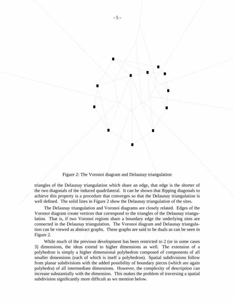
The Voronoi diagram [Vo] is built from a set of input points, called sites.Corresponding to each site is the set of points of Ed which are closer to that site than toany other site. For example, the dotted lines in Figure 2 give the Voronoi diagram for theset of sites shown triangulated in Figure 1. Voronoi diagrams can be used to solve vari-ous nearest neighbor problems. For example, the sites might represent positions where acommodity is available. The region corresponding to a given site would then representthose points from which this is the site of choice for getting the commodity. Or, wemight want to find for each site, the other site to which it is closest.

The Delaunay triangulation [De] is also constructed from a set of sites. In the plane,we build a triangulation of a point set by connecting pairs of sites. This technique can beused to generate an exponential number of different triangulations. For many applica-tions, some of these triangulations are preferable to others. For example, triangulationswhere triangles are more nearly equilateral are often more desirable than those havingmany long skinny triangles. We can capture this property by asking for the triangulationwhich has the largest smallest angle. And, the triangulation which achieves this is theDelaunay triangulation.

The Delaunay triangulation is defined by requiring that no site lie within the cir-cumscribing circle of any triangle of the triangulation. Alternatively, for any two

- 5 -

Figure 2: The Voronoi diagram and Delaunay triangulation

triangles of the Delaunay triangulation which share an edge, that edge is the shorter ofthe two diagonals of the induced quadrilateral. It can be shown that flipping diagonals toachieve this property is a procedure that converges so that the Delaunay triangulation iswell defined. The solid lines in Figure 2 show the Delaunay triangulation of the sites.

The Delaunay triangulation and Voronoi diagrams are closely related. Edges of theVoronoi diagram create vertices that correspond to the triangles of the Delaunay triangu-lation. That is, if two Voronoi regions share a boundary edge the underlying sites areconnected in the Delaunay triangulation. The Voronoi diagram and Delaunay triangula-tion can be viewed as abstract graphs. These graphs are said to be duals as can be seen inFigure 2.

While much of the previous development has been restricted to 2 (or in some cases3) dimensions, the ideas extend to higher dimensions as well. The extension of apolyhedron is simply a higher dimensional polyhedron composed of components of allsmaller dimensions (each of which is itself a polyhedron). Spatial subdivisions followfrom planar subdivisions with the added possibility of boundary pieces (which are againpolyhedra) of all intermediate dimensions. However, the complexity of description canincrease substantially with the dimension. This makes the problem of traversing a spatialsubdivision significantly more difficult as we mention below.

- 6 -

The Voronoi diagram and Delaunay triangulation can be defined in higher dimen-sions as they were above. For the Voronoi diagram regions are now polyhedra (ratherthan polygons) composed of those points closest to a site. The Delaunay triangulation isnow composed of d-simplices. A d-simplex is defined recursively by adding to a d − 1simplex an additional point which is linearly independent of the others and connecting itto all points of the d − 1 simplex. For example, a 2-simplex is a triangle and a 3-simplexis a tetrahedron. Now, the Delaunay triangulation is composed of simplices defined sothat no additional site lies within their circumscribing d-sphere. Finally, the Voronoidiagram and Delaunay triangulation of a set of sites represented as graphs are duals in alldimensions. For further details, see [Ed1].

We conclude this section with one further observation relating the Delaunay tri-angulation (and so, also the Voronoi diagram) to the convex hull. If we are given a set ofsites in Ed and wish to compute their Delaunay triangulation, we can do so by replacingthe sites by a new set of points in Ed + 1. Then, we compute the convex hull of thesepoints. Finally, the Delaunay triangulation can be derived from the projection of thisconvex hull back to Ed. For further details on this derivation, see [Ed1].

2.3. Towards implementation

Having established sufficient background for Voronoi diagrams, Delaunay triangu-lations, and convex hulls, it remains to discuss the difficulties encountered with turningthis theory into practice. As the results mentioned above appeared, implementationsslowly followed. The Graham algorithm for computing convex hulls was easily imple-mented as an extension of a sorting algorithm. However, algorithms for computing the2D Voronoi diagram and Delaunay triangulation and the 3D convex hull ran into prob-lems. It was hard to find an appropriate data structure to represent the geometry. Thesedifficulties arose because incidence relationships become more complex in the nextdimension. It is no longer the case that a vertex (or face) has fixed degree. Indeed, whilewe can control one of these quantities (as in the case of a triangulation), we cannot con-trol both.

Baumgart [Ba] observed that for storing and manipulating planar subdivisions, theedge was the appropriate structure from which to record incidences. In particular, anedge of a planar subdivision connects exactly 2 vertices and separates exactly 2 faces.Baumgart implemented a winged edge structure where an edge stores this topologicalinformation. Each vertex (resp. face) records an edge of which it is an endpoint (resp.which belongs to it). This is sufficient to trace all edges adjacent to a vertex and alledges bounding a face in either order. In Figure 3, we show the basic winged edge struc-ture. The thick edge stores information about the vertices it joins, the faces it separatesand the edges adjacent for each vertex-face pair.

The Baumgart scheme provides an excellent starting point for representing subdivi-sions. In order to become fully useful, it must be enhanced in a few directions. It hasdifficulty representing subdivisions involving holes. It unnecessarily differentiatesbetween the primal and dual representations of a subdivision (as defined e.g. by theVoronoi diagram and Delaunay triangulation). And, it hasn’t defined concise primitivesfor moving around a subdivision.

- 7 -

Face 0 Face 1

Vertex 0

Vertex 1

Edge 0 0

Edge 1 0

Edge 0 1

Edge 1 1

Figure 3: The winged edge data structure

For example, the subdivision shown in Figure 4 (where the dark regions are holes)is difficult to manipulate using winged edge methods. In particular, it is difficult to tracethe edges adjacent to the vertex in the middle. This is because the holes give no gui-dance about their boundaries and so we cannot get attachable pieces of the boundaryeasily.

Figure 4:Winged edge structure can’t represent this

In practical terms, a data structure’s value is measured as the complexity of imple-menting a Voronoi diagram algorithm within it. Prior to the work I am about to describe,applications requiring Voronoi diagrams were typically done using naive techniques(requiring O(n2 ) algorithms) rather than the O(n log n) algorithms I mention here.

- 8 -

Guibas and Stolfi [GS] provided an elegant extension to the winged edge structure.They begin with the observation that an edge potentially performs 4 tasks. It acts as aconnector for 2 vertices and as a separator for 2 faces. In performing each of these tasks,the edge is involved in a ring of edges. These edges might reach to the neighbors of avertex or define the boundary of a face. Each of these rings is stored as a doubly linkedlist of edges. For each edge, the rings to which it belongs are recorded.

They then define operators to let an edge serve in its 4 roles. Thus, we can walkaround an edge ring finding the next edge in the given orientation around the given ver-tex or face. It is also possible to move from one edge ring to another. For example, wecan start at the edge ring corresponding to edges adjacent to a given vertex. We can thenmove to the edge ring of edges adjacent to the face of which the vertex and current edgeare a part. We will describe this process in further detail below. Their structure is calledthe quad-edge and easily stores the Delaunay triangulation and Voronoi diagramtogether.

The storage schema for the quad edge structure considers an edge e as joining anOrigin to a Destination and separating Left and Right bounding faces. They define theprimitive operators Org, Dest, Left, and Right to extract these components of the edge.

Edges come in equivalence classes of 4. For the winged edge shown in Figure 3,we have the four equivalent representatives:

1. The edge from Vertex 0 to Vertex 12. The edge from Face 0 to Face 13. The edge from Vertex 1 to Vertex 04. The edge from Face 1 to Face 0

The first of these is the edge we represented in the original figure. The third is the sameedge pointing in the opposite direction. The second and fourth represent edges which aredual to these edges. Since all four edges are treated alike, there is no longer a notion ofprimal and dual edges. They define primitive operators Rot, Sym, and Flip for movingamong these four components.

These operators combine to provide the facility to navigate easily between a subdi-vision and its dual. We can also explore the subdivision locally tracing the edges arounda vertex or face. To extend our travel to other vertices or faces we need to go from onequad edge equivalence class to another.

To do so, we naturally think of oriented edge rings about vertices and faces. Forexample, the quad-edge shown in Figure 3 may be a part of 4 edge rings. Traversingthese edge rings can be done in either the positive (ie counterclockwise) or negative (ieclockwise) direction. For example, the ring of edges about Vertex 1 has Edge 1 0 as it’sfirst element in a positive traversal and Edge 1 1 as its first element in a negative traver-sal.

The primitives ONext(e) and Oprev(e) are defined to give next and previous edgesin the oriented edge ring about the Origin of the edge e. Similarly, we can talk about theedge ring bounding Face 1. Edge 1 1 and Edge 0 1, the neighboring edges to e in this edgering, are computed as RNext(e) and RPrev(e) in similar fashion. Other operators can bedefined to trace Next and Previous neighbors around the Destination vertex and Left face.These tools for defining quad edges and manipulating edge rings require less than 20

- 9 -

lines of C code [Dw1] to implement.

From these primitive components, Guibas and Stolfi derive an algebra of relationsamong the operators. This algebra allows them to build sophisticated procedures fromrepeated applications of their primitive operators. A key procedure implements theSplice operator allowing us to combine and separate subdivisions. This is their majorconstruction tool. The operator MakeEdge is a simple memory manager able to createan isolated new edge that can later be spliced to a subdivision. These two operators canbe implemented in fewer than 50 lines of C code [Dw1].

Finally, there is the problem of using this derivation productively. The previousparagraphs describe the primitives necessary for manipulating the topology of subdivi-sions. What about the geometry, as would be required for Voronoi diagrams or Delaunaytriangulations? Guibas and Stolfi provide a single geometric primitive which isolates allnumerical computation involved in computing these structures. This primitive InCircledetermines whether its fourth argument lies within the circle defined by its first 3 argu-ments. Using InCircle and the above techniques, the Delaunay triangulation can now beimplemented in 50 additional lines of C code.

The elegance of the Guibas Stolfi structure and its ease of implementation have hadsignificant impact on the application of Delaunay triangulations and Voronoi diagrams.Students in beginning computational geometry courses are able to implement their algo-rithm. Previously, this was a research topic. Others have extended the derivations to findeven more efficient algorithms for computing Delaunay triangulation ([Dw2]).

There remains the problem of extending the Guibas Stolfi structure from 2 to higherdimensions. The basic problem is how to replace the quad edge element. In the plane, itwas sufficient to consider our basic element as an edge and to consider the edge rings towhich that edge belonged. By traversing these edge rings we were able to explore andbuild the subdivision. In higher dimensions, we again have a basic element. The newbasic element will again represent an equivalence class and we define primitive operatorsto enable us to traverse its elements. The element must also belong to rings of edges andfacets which can be traversed to explore the full subdivision. Finally, we need primitiveswhich supports procedures for creating basic building blocks and splicing pieces togetherto build an entire subdivision. Dobkin and Laszlo [DLa, La] have considered the prob-lem in 3 dimensions and Brisson and Lienhardt [Br, Li] give general solutions in alldimensions. We will restrict our attention in what follows to the 3 dimensional case.

In 3 dimensions, our primitive element is the facet-edge pair. This consists of anedge and one of the facets (ie polygons) to which it is adjacent. Just as an edge in 2Dconnected two vertices and separated 2 faces, a facet-edge pair in 3D connects 2 verticesand separates 2 polyhedral regions. Here we must also represent the facet-edge pair dualto our primitive element representing the added complex that came from moving adimension higher. Another difference is that a ring for a facet-edge pair always involves2 rings, the ring of facets about its edge and the ring of edges about its facet. Givenorientations in both the facet ring and the edge ring, we are able to define operatorsPpos(fe) and Pneg(fe) as the neighboring polyhedra for a facet-edge fe in a manneranalogous to RNext(e) and LNext(e) for an edge e in the quad-edge scheme.

Beyond these additional complexities, facet-edges work in a fashion similar toquad-edges. There remains a Splice operator to combine or break pieces. Splice uses the

- 10 -

quad-edge structure to manipulate the 2 dimensional components of a 3 dimensionalstructure. Also, constructing basic elements is more complicated in order to handle theadditional possibilities. However, it is still possible to build all the operators needed tocreate, manipulate and traverse 3 dimensional cell complexes in fewer than 1000 lines ofC code.

Implementing Delaunay triangulations and Voronoi diagrams in 3 dimensions ismore complex than the 2 dimensional process. Algorithms in 2 dimensions either relyupon recursive techniques (i.e. divide and merge as done by [GS]) or iterative techniques(e.g the sweepline algorithm of Fortune [Fo] discussed below). These algorithmssucceed by building data structures to store information that is essentially 1 dimensional.For the divide and merge algorithms, this is the monotonic piecewise linear dividing line.For the sweep algorithms, it is the sweepline itself. Neither paradigm easily extends adimension higher. Further, numerical instabilities become more of a problem as wemove to 3 dimensions.

The InCircle primitive we used in 2D gives way to a InSphere primitive in 3D.Naive implementation of this primitive involves comparing sums of products of quadru-ples of inputs. Even for double precision computations, this computation can be unstablein the face of roundoff errors. Recently, Beichl and Sullivan [BS] have produced a codewhich solves these problems and gives adequate performance. They build the Delaunaytriangulation in a shelling order using the QR technique of matrix factorization in anessential manner to handle problems of rounding. As was the case in dimension 2, it islikely that further research will build upon their work ultimately resulting in simpleimplementations.

2.4. Applications of Voronoi Diagrams and Delaunay Triangulations

The Delaunay triangulation and the subdivisions it induces often arise in practicalproblems. Typical applications require a subdivision of a portion of space. Vertices ofthe subdivision might represent points at which data has been sampled (either physicallyor computationally). Facets of the subdivision might represent homogeneous regions ofspace with respect to some computation. Theoretical results of computational geometryare often used to show that the Delaunay is the appropriate triangulation. Algorithmicdevelopments as described above are then used to create and traverse the Delaunay tri-angulation. In other situations, properties of the Delaunay triangulation are used to jus-tify the use of a simple algorithm by verifying that it yields the correct solution. Wedescribe here a few situations which use these ideas. For further applications and proper-ties of Voronoi diagrams and Delaunay triangulations, see [Au,PS2].

Almgren[Al] considers the problems of finding the surface of smallest area span-ning a wire frame or the surface of smallest area which partitions space into regions ofprescribed volumes. This is a classical problem in the area of minimal surface computa-tion. A discrete approximation to the minimal surface problem involves ‘‘growing’’such surfaces from a soap bubble cluster type geometry. The goal is to understand theproblem in discrete settings and to use these insights as a tool in understanding the con-tinuous case. The soap bubble cluster modeling is done thru a Voronoi cell evolver.This involves a computer program implementing the 3D Voronoi diagram. Combina-torial geometry is created and evolved by moving control sites of several different colors

- 11 -

(one color for each desired cell of the desired final soap bubble cluster). This geometryis used both to compute positions and to create images and videos of this process usingthe techniques of computer graphics. Their work has built upon theoeretical develop-ments relating to the Delaunay triangulation and the data structure of [DLa] is central totheir implementation. This work is central in the field of visualizing mathematicalphenomena. It would not have been possible without the advent of graphics hardwareand computational geometry techniques.

A related application concerns the problem of generating meshes for solving partialdifferential equations. Typical of such situations is that described in [Bak1, Bak2] for thecomputation of inviscid transonic flows over aerodynamic shapes. The goal is to producea triangulation of the space surrounding the aerodynamic shape for which the individualsimplices (in this case tetrahedra) are well behaved. Well behaved tetrahedra allow finiteelement methods to produce stable solutions to the relevant equations. In this case, wellbehavedness is measured as the worst case ratio between side lengths of a giventetrahedron and the radius of the sphere inscribed in the tetrahedron. If this ratio growsas O(1), the triangulation is deemed to be well behaved.

The starting conditions often involve a 2 dimensional triangulation of Delaunay orsimilar form. Various techniques have been given to grow this triangulation into a 3Dmesh. The most common combine the advancing front technique which grows off theinitial triangulation in a conformal fashion with Delaunay techniques. These techniqueshave proved successful as front ends to solvers considering point sets of size 400,000from which they generate meshes of 2.4 million points. Reported computed times for thetriangulation are half an hour on a single processor Cray 2.

A second application involving Delaunay triangulation arises in the problem ofvolume visualization. Max, Hanrahan and Crawfis [Ma] present a technique for visualiz-ing a 3D scalar function. In a typical volume visualization task, data is given at a collec-tion of 3D points and the goal is to provide a useful rendering of the data. The goal is togenerate one or more levels of the image (using transparency) to give a useful view of a3D function. Solving this problem when data come at vertices of a regular cubic latticeis a conceptually easy but computationally intensive task.

The more general case is where data values are allowed to occur at arbitrary posi-tions in space. This is the desired case. In this case, it is necessary to triangulate spacewith vertices defined at positions where we have data values. The transparency calcula-tions now require that we do a process similar to hidden surface removal. A desirable tri-angulation would be the Delaunay for the reasons described previously. This turns out tobe the correct choice due to the acyclicity condition of Edelsbrunner [Ed2] from the com-putational geometry literature.

A practical solution to this problem is to find a well-behaved ordering of the tetrahe-dra. Ideally, such an ordering would have the property that tetrahedron A comes before Bif no part of B is obscured by A with respect to a given view point. Conceptually, thisinvolves considering a subdivision of a region of space and a fixed direction. We thenask if there is always a tetrahedron of the subdivision which can be translated to infinityin the given direction without intersecting any other tetrahedra of the subdivision. Weremove this tetrahedron from the subdivision and repeat the procedure until the subdivi-sion is empty. It is easy to verify that there are subdivisions for which this is not

- 12 -

possible. In such cases, it is necessary to introduce new data values and further subdi-vide, a tedious task. Edelsbrunner [Ed2] shows that this can never be the case if theDelaunay triangulation is used. Max et al [Ma] are able to build a simpler algorithmbecause of this result.

A final application area illustrates the use of properties of the Delaunay triangula-tion in a seemingly unrelated graphics problem. Painter and Sloan [PS1] consider theproblem of successively refining image generation. The goal is to be able to generaterapid images using ray tracing techniques and then to refine the images, as time permits,to higher quality. At the core of their technique is a convolution integral correspondingto their sampling technique. They must build an image function based upon their sam-pling to convolve with the filter function from their technique.

Their approach builds upon an interpolation scheme over the image. Their initialapproach was to use linear techniques for this interpolation. When higher quality wasrequired, they appealed to the properties of Delaunay triangulations to produce a trianglebased interpolation scheme for doing the interpolation. This yields better images becausethe locality properties of the Delaunay triangulation lend themselves to interpolation.They were able to implement their scheme because codes for computing Delaunay tri-angulations in the plane are readily available.

These examples are meant to show how the Delaunay triangulation is used bygraphics based researchers. Note that the applications are to problems unrelated to com-putational geometry. Indeed, most computational geometers are unaware of these prob-lem areas. The techniques of computational geometry were not developed to help theseusers but rather were developed in a broader context of basic research. As research incomputational geometry has matured, researchers in other fields have been able to applythis basic research to their problems. The Delaunay triangulation is a classic example ofthis situation. Other example also exist and will continue to grow as the fields of compu-tational geometry and computer graphics prosper.

Further extensions of the Delaunay and other triangulations are being developed tohelp handle situations where the applications often drive the theory. Typical problemsask for the smallest number of points that can be added to a point set to produce a tri-angulation having a desired property.

For example, consider the problem of producing a triangulation having no obtuseangles since these angles can cause problems for interpolation. Bern and Eppstein showthat the addition of a polynomial number of points is always sufficient to generate such atriangulation [BE]. Another problem is that the Delaunay triangulation of n points in E3

may have size O(n2 ). It is natural to ask whether we can add points to the set to reducethe size of its Delaunay triangulation. Surprisingly, it is possible to add O(n) points andachieve a Delaunay triangulation of size O(n) [BEG].

3. Algorithmic paradigms from Computer Graphics

- 13 -

3.1. The Basic Techniques

A central problem in computer graphics is the development of realistic renderingsof complex scenes. In the 1960’s, this quest led to the consideration of algorithms foraccurately rendering 3 dimensional scenes on a graphics display. One requirement is theelimination of hidden lines or hidden surfaces from a 3 dimensional model. The first suc-cessful approaches extended existing paradigms to geometric domains. These extensionsinitiated important areas of research in computational geometry. The results of thisresearch have found new applications in computer graphics. We explore two solutions tothe hidden surface problem and show how they were generalized.

In its simplest form, hidden surface removal considers a 3 dimensional scene con-structed from polygons and asks (for given viewing conditions) which parts of the sceneappear on a flat display. For our purposes, we can assume that all viewing transforma-tions and projection have been done. All polygons have been triangulated so that ourinput is a set of possibly overlapping triangles in the plane from which the visible imageis to be constructed. The triangles contain additional information from which it is possi-ble to determine which of a pair of triangles is closer to the viewer (and so is visible).The hidden surface removal problem is then to identify the visible triangles and parts oftriangles.

Two popular early algorithms for this problem were the scan line algorithm of Wat-kins [Wat] and the space subdivision algorithm of Warnock [War]. These algorithmsextended existing paradigms in algorithm design to the geometric realm. Scanline algo-rithms are sophisticated extensions of for-loop type constructions available in program-ming languages. Area subdivision algorithms are applications of simple recursion.

The Watkins scan line algorithm identifies events that will occur during the compu-tation and orders them. Events are situations where the set of visible triangles changes.These changes come about from the appearance of new triangles or the intersection ofexisting triangles. Ordering is with respect to the y-coordinates at which events occur.Events are ordered in order of increasing y-coordinate. A data structure is maintainedbetween events and updated to allow for efficient processing of individual events.

The scanline processing begins with the sorting of y-coordinates of all input trian-gles. Then there are then 3 types of events. First, a triangle might be inserted or deleted.Otherwise, a triangle might change it edges of interest. This occurs when the middle (interms of y-coordinates) vertex is encountered. Finally, edges of existing triangles mightintersect. Events of the first 2 types can be determined by the initial sort. Events of thethird type must be identified as the algorithm proceeds. It is possible to do so efficientlybecause triangle edges can only intersect if they belong to triangles that are adjacent inour data structure. Hence, by maintaining an ordering of triangles and tracking changesin the ordering, we can identify events of the third type. The mathematical basis for scanline algorithms of this type can be traced back at least as far as the work of Hadwiger[Ha].

Area subdivision algorithms make powerful use of basic ideas. Initially, the planeis considered as a single rectangle. And, the triangles of this rectangle are considered asthe set of all input triangles. Then, a recursive procedure goes as follows:

- 14 -

foreach existing rectangleif the rectangle intersects no triangles

Color the rectangle with the background color and return.else if the rectangle intersects 1 triangle

Output the triangle clipped to the borders of the rectangle andreturn.

if the rectangle is completely covered by some triangle(s)Remove all triangles which lie behind the frontmost covering tri-angle.

if this leaves only 1 triangle intersecting the rectangle,Output that triangle suitably clipped and return.

else if more than 1 triangle remains in the rectangle,subdivide the rectangle into 4 subrectangles, determinewhich triangles intersect each subrectangle and recur.

This recursion terminates when the complete picture (as a set of monochrome triangles)has been created.

3.2. Further extension of scanline techniques

Scanline techniques of computer graphics were so named because of their connec-tion to actual graphics hardware. These techniques found application to raster deviceswhich create their image by refreshing the screen a scanline at a time. When movedfrom discrete raster space to continuous Euclidean space, they were renamed as sweep-line techniques. In part, it was possible to perform this extension with only minimalmodification of the methodology mentioned above. However, as the class of problemsamenable to this technique grew, it was necessary to further extend the technique. Toexplore the possibilities, I briefly describe 2 algorithms built upon sweepline algorithms.

First, we consider one of the earliest uses within computational geometry of thesweepline paradigm. Shamos and Hoey [SH2] considered the problem of determiningwhether any 2 of a collection of n line segments have a point in common. To understandtheir algorithm, imagine that all n segments were drawn in the plane and that we sweptacross them with a vertical line. Imagine that as the vertical line sweeps across the plane,it keeps track of the order in which the segments intersect it from bottom to top. Notethat not all segments will intersect it in each of its placements. Now, suppose that thevertical line encounters a pair of intersecting segments. It must be the case that immedi-ately before their intersection, the two segments were adjacent in the ordering of inter-sections with the sweep line. Immediately after their intersection, they were also adja-cent but their order had reversed. From this observation, we conclude that only line seg-ments that are adjacent in their intersection with the vertical line must ever be tested forintersection. This would give us the events as discussed for scanline algorithms. Unfor-tunately, it is inefficient to consider all orders of segments along the vertical line as itsweeps. There may be O(n2 ) such orderings in the general case and O(n) orderings oflength n even in the case where no pair of segments intersect.

- 15 -

What remains is the crux of the Shamos-Hoey algorithm, the determination of theevents at which tests must be performed. They begin their algorithm by sorting the 2nendpoints of the n original line segments based upon their x-coordinates. Having doneso, they observe that the order of segments only changes in a meaningful way when anew segment begins or an existing segment ends. In the case of an insertion, the execu-tion of the event is to determine if the new segment intersects either of its neighbors.And, in the case of a deletion, the execution of the event is to determine if the neighborsof the existing segment (ie 1 above and 1 below) ever intersect one another. Their algo-rithm correctly determines if there is an intersection among the line segments. It can dono more. That is, it cannot guarantee to find the first intersection or determine the correctnumber of intersections. By maintaining balanced trees of segments and doing appropri-ate sorting, their algorithm can be made to run in time O(nlogn). This time is provablyoptimal [PS1].

An extension of the sweepline algorithm proposed by Shamos and Hoey was givenby Bentley and Ottman a few years later. They consider the extension to finding all pos-sible intersections rather than merely determining if an intersection existed. To do so,they have to modify the sweepline algorithm to enable them to determine events ‘‘on-the-fly’’. Their algorithm has a running time of O(nlog n + klog n) where k is thenumber of intersections reported. Full details are in [BO, PS].

The Bentley Ottman algorithm is not asymptotically optimal. Because it reportsintersections in order based upon their x coordinate, it must sort all intersections and socannot finish in the desired optimal time bound O(n log n + k). Achieving this timebound was an open problem for a decade. In order to reduce the complexity, it wasnecessary to produce a sweepline algorithm which modified its sweep direction torespond to the data it was encountering. Such a technique, called topological sweep wasdeveloped initially for the problem of planar subdivision searching [Ed1]. Chazelle andEdelsbrunner[CE] were then able to extend it to give an optimal algorithm for the prob-lem of reporting all intersecting segments. Their algorithm while more complex thanthose presented here, represents a significant theoretical breakthrough. They have imple-mented a version of their algorithm. As topological sweep and its extensions are morefully understood, we can expect new versions of the sweepline algorithm that find appli-cation to computer graphics problems of practical importance as well.

There are other extensions to sweepline algorithms which have appeared in thecomputational geometry literature. The Voronoi diagram algorithm of Fortune [Fo] isone that extends the paradigm and yields an immediately practical algorithm. Until hisalgorithm appeared, there were known techniques for finding the Voronoi diagramoptimally through the use of recursion but no optimal incremental method was known.Incremental methods tend to be more robust for computational purposes.

The difficulty with computing a Voronoi diagram via a sweepline method is thatthe events begin to occur before they can be predicted. Consider a sweep across theVoronoi diagram of Figure 2 with a horizontal line. Voronoi regions are encounteredbefore the site to which they correspond has been encountered. This deterred earlyefforts at creating Voronoi diagrams by sweep methods. Fortune circumvents thisdifficulty by redefining the distance function. His new distance function has the twonecessary properties. First, a Voronoi region is not encountered by a vertical sweeplineuntil its site is encountered. Next, the topology of the diagram is the same as that of the

- 16 -

‘‘correct’’ diagram. His modification to the sweepline paradigm can be viewed as ameans of modifying computational techniques so that the paradigm holds for a broaderclass of problems.

The examples given here are meant to give a flavor of the impact that the originaltechnique of Watkins (or previously Hadwiger) has had on computational geometry.Also, we can see that as the techniques get improved and refined, they will have evenmore significant impact on computer graphics. There are numerous other exampleswhere a sweepline is allowed to having non-trivial shape or where sweeping is done by aplane or higher dimensional object. Many of these examples aim at efficient solutions togeneralizations of the hidden surface removal problem which originally motivated Wat-kins. The articles [Ber, Ya] provide pointers into this vast literature.

3.3. Extending the area subdivision paradigm

The area subdivision technique proposed by Warnock built upon pre-existing ideas.For a survey of the rich history of these idea, see Samet’s excellent books on the subject[Sa1, Sa2]. Within the computational geometry community, these ideas were developedas an alternative method to the searching techniques described in the previous section.As this development proceeded, generalizations were developed which have since foundsignificant application in the graphics community. We will describe here briefly thedevelopments which led to the k − d tree, the quadtree, the octree and their application.

The subdivisions above lend themselves to asymptotically efficient searchingschemes. However, the difficulty of searching on existing boundary elements can resultin an overly complicated search scheme. In response to such problems, Bentley [Ben]developed an algorithm which was asymptotically less efficient but practically moreimplementable. He considered the problem of organizing a point set in Ed for varioussearches and proposed a method of creating the k − d (i.e. k-dimensional) search tree.

We describe here a 2 − d tree. Imagine that we are given a set of points in the planeand wish to preprocess them for easy searching. We wish to devise a scheme for generat-ing easily used search trees. The 2 − d tree in this case consists of internals nodes atwhich queries are asked and frontier nodes holding data. The interior nodes aresimplified to only contain queries of the form x i :v which determine whether the ith coor-dinate of the query point is less than, equal to or greater than the value v. Comparisonsof this type then cause us to take a left, middle or right branch in the search tree. Thequeries are organized to alternate the value of i, the coordinate of the query point beingprobed. And, the value of v is chosen as the median among all possible values. Usingthese ideas, building and searching a k − d tree becomes an easy exercise. An improvedimplementation for k − d trees for nearest neighbor searching is given in [Sp].

Schemes for implementing k − d trees for dimensions 2 and 3 have been studied innumerous contexts. The 2 dimensional versions are a variant of the quadtree searchstructure which arose from Warnock’s original algorithm. The 3 dimensional versions ofquadtrees are called octrees. Quadtrees (and octrees) differ slightly from k − d trees. Theformer are built by dividing space in half. The latter are built by dividing a point set inhalf. Quadtrees tend to perform well in practice since scenes are typically uniformly dis-tributed. The assumptions underlying k − d trees make it possible to prove that worst casebehavior, which can be significantly worse than optimal, will not occur for such scenes.The development and application of these simple ideas to a significant number of

- 17 -

problems in computational geometry and computer graphics has been remarkable.

These structures play a central role in various ray tracing and volume visualizationtechniques of computer graphics. For example, a ray tracer will build an octree from theobjects in the scene it is tracing making it possible to test a ray against a small number ofobjects (rather than the entire scene) to find its first intersection. Arvo and Kirk [AK]have extended these ideas even further using the 5 dimensional version of such trees tofurther speed ray tracing. In the ray tracing problem, one (or more) rays is traced foreach pixel of an output scene. Arvo and Kirk observe that these rays can be classified bytheir origin (a point x,y,z in E3) and direction (represented by the angle pair (θ ,φ)). Oncea ray in a given direction has been traced, the results of this trace can be stored in a5 − tree that can be searched by future rays in the given direction. These ideas combinedwith a clever storage scheme lead to an efficient algorithm.

Others have extended these ideas for the problem of volume visualization. Here theinput is represented as the combination of a subdivision and an array of 3D data samplescalled voxels. Octrees have been used productively in this environment as the basis ofmany image creation algorithms. The goal is to use the input data in combination withviewing parameters to generate one or (typically) multiple views of the data. Typicalapplications are to computational fluid dynamics and medical imaging. The octree isbuilt from the data and then probed by the ray tracing algorithm. For examples, see [Ne,Wi].

Within the computational geometry study of such problems, there have beennumerous range searching extensions of k-d trees. Recent results here apply deep resultsfrom probability theory (dealing with the Vapnik-Chervonenkis dimension) to obtaintheoretical improvements [EW]. Other results give methods of extending range search-ing techniques to more sophisticated queries [DE].

4. Conclusions and further results

This paper has shown that the fields of computational geometry and computergraphics have had significant impact on one another. Indeed, a major frustration in writ-ing this paper is that few of the exciting interactions can be explored. The two problemswe considered -- spatial subdivision creation and exploration and hidden surface removal-- lie at the core of both computational geometry and computer graphics. Two otherproblems must be mentioned to round out the picture. We do so in this section.

4.1. Precise practical computation

Historically, computational geometry papers have assumed that the data they sawon input was ‘‘well-behaved’’ and that the computations they did were very stable. Thismeant, for example, that points in the input set were sufficiently separated, no triple ofinput points was on the same line and no triple of input lines contained the same point.Furthermore, all intermediate computations were done in infinite precision arithmetic sothat roundoff error was never a problem. Geometers justified these assumptions on thebasis that they eliminated unnecessary complications that could easily be fixed. Simi-larly, graphics programmers would occasionally observe glitches in their pictorial outputwhich they attributed to problems with floating point computations. Typically, theywould find ad hoc techniques which would enable them to work around these glitchesand produce ideal output.

- 18 -

As computer speed increases and our appetite for more sophisticated inputsincreases, we can no longer assume that inputs are well behaved or that computations aredone at infinite precision or that ad hoc techniques will always be available to help solveour problems. This creates the need for a more thorough study of the problem. It isnecessary to isolate the exact parts of the problem where numerical problems occur andto determine the effect they will have on the ultimate solution.

Three approaches have been followed in exploring this problem. In [EM], a methodis presented to perturb the input to create a new input set which will be well behaved andyield the same result. This is done by perturbations large enough to avoid degeneratesituations even in the face of finite precision computations but small enough so that theanswer to the problem does not change. Other approaches involve backward error ana-lyses. Here, we determine the precision at which computations must be done given theinput precision and the nature of the computation [SSG, FM, Bar]. A third approach con-siders the problem of building a tracker which follows the computation and determinesthe precision as the computation proceeds [DS]. The idea is to detect when insufficientprecision remains and backtrack to a point whence the computation can be redone at ahigher precision.

4.2. Decomposition of polygons and polyhedra

A recurrent theme in computer graphics is the modeling and rendering of complexobjects. These problems often depend upon techniques for subdividing individualobjects or the space of entire scenes. In the former problem, the goal is to represent anobject as a formula built in terms of primitive components. In the latter, we might wantto render a scene in a sorted order by appropriate subdivision of space into regions eachinvolving only a single object. Each of these problems arose in the computer graphicsliterature. And, each has motivated research in computational geometry.

Peterson [Pet] proposed the problem of representing a polygon or polytope as a res-tricted CSG formula. His goal was to have a representation that consisted of intersec-tions and unions of halfplanes (or halfspaces) of support of the edges (or faces) of the ori-ginal object. He showed that such a monotone representation of an arbitrary simplepolygon was possible by a formula which used each halfplane exactly once. Others haveextended his work to show that such a formula can be computed in O(nlogn) time. It hasalso been shown that no such formula exists for polytopes unless face halfspaces arerepeated. See [DGHS,PY,Dey] for details.

The binary space partition tree was introduced in [Fu] as a scheme for fast renderingof scenes in computer graphics. This is a scheme for creating a binary tree correspondingto a scene of polygons. The nodes of the tree are planes of support of individualpolygons. These nodes are meant to subdivide the scene into two nearly equal partscorresponding to the objects in each half space as defined by the partition plane. Thisproblem was extended by [PY] to the general problem of finding a collection of arbitraryplanes to subdivide a general scene. They show that a partition of size O(nlogn) for nedges in the plane. They also show a partition of size O(n2 ) for n planar facets in E3.Furthermore, they show that this result is the best possible.

- 19 -

Acknowledgements

It is a pleasure to thank Brad Barber and three anonymous referees for numerouscomments which improved the readability of this manuscript.

5. References

[Al] Almgren, F., ‘‘The geometric calculus of variations and modeling naturalphenomena’’, Proceedings of the Workshop on Statistical thermodynamicsand differential geometry of micro-structured material, Institute forMathematics and Its Applications, Springer-Verlag, New York, 1991

[AK] Arvo, J. and Kirk, D., ‘‘Fast ray tracing by ray classification’’, ComputerGraphics, vol. 21, 1987, pp. 55-64.

[Au] ‘‘Voronoi diagrams -- A survey of a fundamental geometric data structure’’,ACM Computing Surveys, 23, 1991, 345-405.

[Bak1] Baker, T.J., ‘‘Automatic mesh generation for complex three-dimensionalregions using a constrained Delaunay triangulation’’, Engineering with Com-puters, 5, 1989, 161-175.

[Bak2] Baker, T.J., ‘‘Unstructured meshes and surface fidelity for complex shapes’’,AIAA Tenth Computational Fluid Dynamics Conference, Hawaii, 1991.

[Bar] Barber, C. B., ‘‘Computational geometry with imprecise data and arith-metic’’, PhD Thesis, Department of Computer Science, Princeton Univer-sity, June, 1992.

[Ba] Baumgart, B., ‘‘A polyhedron representation for computer vision’’, 1975National Computer Conference, AFIPS Conference Proceedings, vol. 44,AFIPS Press, 1976, pp. 589-596.

[BS] Beichl, I. and Sullivan, F., ‘‘A C program for computing 3D Delaunay tri-angulations’’, unpublished software.

[Ben] Bentley, J.L., ‘‘Multidimensional binary search trees used for associativesearching’’, Communications of the ACM, 18, 509-517, 1975.

[BO78] Bentley, J.L. and Ottman, Th., ‘‘Algorithms for reporting and countinggeometric intersections’’, Carnegie-Mellon University, August 1978.

[Ber] Bern, M., Dobkin, D., Eppstein, D., and Grossman, R., ‘‘Visibility with amoving point of view’’, Proceedings of the First Annual ACM-SIAM Sympo-sium on Discrete Algorithms, 1990, 107-117.

[BE] Bern, M. and Eppstein, D., ‘‘Polynomial-size nonobtuse triangulation ofpolygons’’, Proceedings of the ACM Symposium on ComputationalGeometry, 1991, pp. 342-350.

[BEG] Bern, M., Eppstein, D. and Gilbert, J., ‘‘Provably good mesh generation’’Proceedings of the IEEE Symposium on Foundations of Computer Science,1990, pp. 231-241.

[Br] Brisson, E., ‘‘Representing geometric structures in d dimensions: topologyand order’’, Proceedings of the ACM Symposium on ComputationalGeometry, 1989, pp. 218-227.

- 20 -

[CE] Chazelle, B. and Edelsbrunner, H., ‘‘An optimal algorithm for intersectingline segments in the plane’’, Proceedings of the IEEE Symposium on Foun-dations of Computer Science, 1988, pp. 590-600.

[Dey] Dey, T., ‘‘Triangulation and CSG representation of polyhedra with arbitrarygenus’’, Proceedings of the ACM Symposium on Computational Geometry,1991, pp. 364-372.

[De] Delaunay, B., ‘‘Sur la sphere vide’’, Izv. Akad. Nauk SSSR, OtdelenieMatematicheskii i Estestvennyka Nauk, vol. 7, 1934, pp. 793-800.

[DE] Dobkin, D. P. and Edelsbrunner, H., ‘‘Space searching for intersectingobjects’’, J. Algorithms, vol. 8, 1987, pp. 348-361.

[DGHS] Dobkin, D., Guibas, L., Hershberger, J., and Snoeyink, J., ‘‘An efficientalgorithm for finding the CSG representation of a simple polygon’’, Com-puter Graphics, vol. 22, 1988, pp. 31-40.

[DLa] Dobkin, D. and Laszlo, M.J., ‘‘Primitives for the manipulation of three-dimensional subdivisions’’, Algorithmica, vol. 4, 1989, pp. 3-32.

[DL1] Dobkin, D.P. and Lipton, R. J. , ‘‘On some generalizations of binarysearch’’, Proceedings of the 6th ACM Symposium on the Theory of Com-puting, 310-316, 1974.

[DL2] Dobkin, D. and Lipton, R., ‘‘Multidimensional search problems’’, SIAM J.Computing, vol. 5, 1976, pp. 181-186.

[DS] Dobkin, D. and Silver, D., ‘‘Applied computational geometry: towardsrobust solutions of basic problems’’, JCSS, vol. 40, 1990, 70-87.

[Dw1] Dwyer, R. A., Software for computing Delaunay triangulation, 1987.

[Dw2] Dwyer, R. A., ‘‘A faster divide-and-conquer algorithm for constructingDelaunay triangulations’’, Algorithmica, vol. 2, 1987, pp. 137-152.

[Ed1] Edelsbrunner, H., Algorithms in Combinatorial Geometry, Springer-Verlag,New York, 1987.

[Ed2] Edelsbrunner, H., ‘‘An acyclicity theorem in cell complexes in d dimen-sions’’, Proceedings of the ACM Symposium on Computational Geometry,1989, pp. 145-151.

[EM] Edelsbrunner, H. and Mucke, E., ‘‘A technique to cope with degeneratecases in geometric algorithms’’, Proceedings of the ACM Symposium onComputational Geometry, 1988, pp. 118-133.

[Fo] Fortune, S. ‘‘A sweepline algorithm for Voronoi diagrams’’, Algorithmica,vol. 2, 1987, pp. 153-174.

[FM] Fortune, S. and Milenkovic, V., ‘‘Numerical stability of algorithms for linearrangements’’, Proceedings of the ACM Symposium on ComputationalGeometry, 1991, pp. 334-341.

[Fu] Fuchs, H., Kedem, Z., and Naylor, B., ‘‘On visible surface generation by apriori tree structures’’, Computer Graphics, vol. 14, 1980, pp. 124-133.

[Gr1] Graham, R., ‘‘An efficient algorithm for determining the convex hull of afinite planar set’’, Information Proc. Letters, vol. 1 , 1972, pp. 132-133.

- 21 -

[Gr2] Graham, R., private communication, 1987.

[GS] Guibas, L. and Stolfi, J., ‘‘Primitives for the manipulation of general subdi-visions and the computation of Voronoi diagrams’’, ACM Trans. Graphics,vol. 4, 1985, pp. 74.123.

[Ha] H. Hadwiger, ‘‘Eulers charakteristic und kombinatorische geometrie’’, J.Reine und Angew. Math., 1955, vol. 194, pp. 101-110.

[HW] D. Haussler and E. Welzl, ‘‘Partitioning and geometric embedding of rangespaces of finite Vapnik-Chervonenkis dimension’’, Proceedings of the 3rdACM Symposium on Computational Geometry, 1987, pp. 331-340.

[Kn] Knuth, D., The Art of Computer Programming, vol. 3, Addison-Wesley,Reading, Ma., 1973.

[La] M.J. Laszlo, ‘‘A data structure for manipulating three-dimensional subdivi-sions’’, PhD dissertation, Princeton University, 1987.

[Li] P. Lienhardt, ‘‘Subdivision of n-dimensional spaces and n-dimensional gen-eralized maps’’ Proceedings 5th ACM Symposium on ComputationalGeometry, 1989, pp. 228-236.

[Ma] Max, N., Hanrahan, P. and R. Crawfis, ‘‘Area and volume coherence forefficient visualization of 3D scalar functions’’, Computer Graphics, vol. 24,no. 5, 1990, pp. 27-33.

[Ne] Neeman, H., ‘‘A decomposition algorithm for visualizing irregular grids’’,Computer Graphics, vol. 24, no. 5, 1990, pp. 49-56.

[PS] Painter, J. and Sloan, K., ‘‘Antialiased raytracing by adaptive progressiverefinement’’, Computer Graphics, vol. 23, no. 3, 1989, pp. 281-288.

[Pa] Palios, L., ‘‘Decomposition Algorithms in Computational Geometry’’, PhDthesis, Princeton University, Department of Computer Science, March, 1992.

[PY] Paterson, M. and Yao, F., ‘‘Efficient binary space partitions for hidden-surface removal and solid modeling’’, Discrete and ComputationalGeometry, vol. 5, 1990, 485-503.

[Pet] Peterson, D., ‘‘Halfspace representations of extrusions, solids of revolutionand pyramids’’, SANDIA Report SAND84-0572, Sandia National Labora-tories, 1984.

[SSG] Salesin, D., Stolfi, J., and Guibas, L., ‘‘Epsilon Geometry: Building robustalgorithms from imprecise computations’’, Proceedings of the ACM Sympo-sium on Computational Geometry, 1989, pp. 208-217.

[Sa1] Samet, H., The design and analysis of spatial data structures, Addison-Wesley, Reading, 1990.

[Sa2] Samet, H., Applications of spatial data structures: computer graphics, imageprocessing and GIS, Addison-Wesley, Reading, 1990.

[S] Shamos, M.I., ‘‘Geometric complexity’’, Proceedings of the 7th ACM Sym-posium on the Theory of Computing, 224-233, 1975.

[SH1] Shamos, M.I. and Hoey, D., ‘‘Closest point problems’’, IEEE Symposium onfoundations of computer science, 151-162, 1975.

- 22 -

[SH2] Shamos, M.I. and Hoey, D., ‘‘Geometric intersection problems’’, IEEESymposium on foundations of computer science, 208-215, 1976.

[Sp] Sproull, R.F., ‘‘Refinements to nearest-neighbor searching in k-dimensionaltrees’’, Algorithmica, vol. 6, 1991, pp. 579-589.

[Vo] Voronoi, G., ‘‘Nouvelles applications des parametres continus a la theoriedes formes quadratiques’’, Journal fur die reine und angewandte Mathema-tik, 133, 1907, 97-178; 134, 1908, 198-287; 136, 1909, 67-181.

[Wa69] Warnock, J. E., ‘‘A hidden-surface algorithm for computer generated half-tone pictures’’, University of Utah Computer Science Department, TR 4-15,1969.

[Wa70] Watkins, G. S., ‘‘A real-time visible surface algorithm’’, University of UtahComputer Science Department, UTEC-CSc-70-101, June, 1970.

[Wi] Wilhelms, J. and van Gelder, A., ‘‘Octrees for faster isosurface generation’’,Computer Graphics, vol. 24, no. 5, 1990, pp. 57-62.

[Ya] Yao, F.F., ‘‘Computational geometry’’, in Algorithms in Complexity,Elsevier, Amsterdam, 1990, 345-490.