Department of Civil and Environmental Engineering Stanford...
222
Department of Civil and Environmental Engineering Stanford University PERFORMANCE EVALUATION OF VIBRATION CONTROLLED STEEL STRUCTURES UNDER SEISMIC LOADING by Luciana R. Barroso and H. Allison Smith Report No. 133 June 1999
Transcript of Department of Civil and Environmental Engineering Stanford...

Department of Civil and Environmental Engineering
Stanford University
PERFORMANCE EVALUATION OF VIBRATION CONTROLLED STEEL STRUCTURES UNDER SEISMIC LOADING
by
Luciana R. Barroso
and
H. Allison Smith
Report No. 133
June 1999

The John A. Blume Earthquake Engineering Center was established to promote research and education in earthquake engineering. Through its activities our understanding of earthquakes and their effects on mankind’s facilities and structures is improving. The Center conducts research, provides instruction, publishes reports and articles, conducts seminar and conferences, and provides financial support for students. The Center is named for Dr. John A. Blume, a well-known consulting engineer and Stanford alumnus. Address: The John A. Blume Earthquake Engineering Center Department of Civil and Environmental Engineering Stanford University Stanford CA 94305-4020 (650) 723-4150 (650) 725-9755 (fax) earthquake @ce. stanford.edu http://blume.stanford.edu
©1999 The John A. Blume Earthquake Engineering Center

PERFORMANCE EVALUATION OFVIBRATION CONTROLLED STEEL
STRUCTURES UNDER SEISMIC LOADING
by
Luciana R. Barrosoand
H. Allison Smith
The John A. Blume Earthquake Engineering Center
Department of Civil and Environmental Engineering
Stanford University
Stanford, CA 94305
Report No. 133
June 1999

c Copyright 1999 by Luciana R. Barroso
All Rights Reserved
ii

Abstract
The structural engineering community has been making great strides in recent years
to develop performance-based earthquake engineering methodologies for both new
and existing construction. For structural control to gain viability in the earth-
quake engineering community, understanding the role of controllers within the con-
text of performance-based engineering is of primary importance. Design of a struc-
ture/controller system should involve a thorough understanding of how various types
of controllers enhance structural performance, such that the most e�ective type of
controller is selected for the given structure and seismic hazard.
The goal of this research is to evaluate the role of structural control technol-
ogy in enhancing the overall structural performance under seismic excitations. This
study focuses on steel moment resisting frames and three types of possible controllers:
(1) friction pendulum base isolation system, FPS (passive); (2) linear viscous brace
dampers, VS (passive); (3) and active tendon braces, ATB. Two structures are se-
lected from the SAC Phase II project, the three story system and the nine story
system. Simulations of these systems, both controlled and uncontrolled, are prepared
using the three suites of earthquake records, also from the SAC Phase II project,
representing three di�erent return periods. Several controllers are developed for each
structure, and their performance is judged based on both roof and interstory drift,
normalized dissipated hysteretic energy, and peak oor acceleration demands.
This investigation has the following speci�c objectives: (1) To evaluate the ef-
fect of the various controller architectures on seismic demands as described through
performance-based design criteria; (2) To evaluate the sensitivity of the structure-
controller performance based on a variation of control parameters, load levels and
structural modeling; (3) To evaluate di�erent systems using a probabilistic format.
iii
The control parameters investigated for the FPS system include the isolation period
and the coeÆcient of friction. These parameters were varied to span a range of pos-
sible values. For the VS damper system, the e�ect of variation in e�ective damping
and its distribution over the height of the structure were evaluated. A representative
ATB control scheme was then designed with actuator saturation levels comparable
to the VS damper system for comparison.
Results indicate that structural control systems are e�ective solutions that can
improve structural performance. All three control strategies investigated can sig-
ni�cantly reduce the seismic demands on a structure, thereby reducing the expected
damage to the structure. However, no one system is consistently the best at all hazard
levels. The viscous system proves to be the most insensitive to modeling assumptions.
The isolation system can maintain the demands close to the structure's elastic limit.
However, the onset of nonlinear behavior decreases the system's e�ectiveness. The
active system is also sensitive to design assumptions, such as output parameters and
structural model parameters used in design. Peak responses alone do not describe the
possible damage incurred by the structure as cumulative damage results from several
incursions into the inelastic range. Accurate evaluations should involve consideration
of the dissipated hysteretic energy.
For isolation systems, selection of isolation period has the greatest impact in the
resulting seismic demands on the superstructure. Lowering the friction coeÆcient can
cause small reductions in drift demands, but the cost of this reduction in structural
demands is an increase in bearing displacements. This system of control proves to
be very e�ective system for both the 3-Story and 9-Story structures and all three
sets of ground motions. The median response of the superstructure remains close to
elastic even under severe ground motions. This system, however, is sensitive to the
sti�ness of the structure, and its e�ectiveness begins to deteriorate once noticeable
nonlinearities occur.
The viscous damper system is very sensitive to both the amount of e�ective damp-
ing provided and the distribution of dampers over the height of the structure. Di�er-
ent damper distributions have little impact on the roof drift. However, by distributing
dampers according to relative story sti�ness and expected peak plastic deformations,
the drift demands are more evenly distributed among the di�erent stories. If the
dampers are located in only a few stories for the same amount of e�ective damping,
iv
however, the system can be highly ine�ective and may increase story demands at
stories without dampers.
The capacity of the actuators for the ATB system contributes greatly to the
e�ectiveness of the control system. Higher actuator capacities provide the controller
a greater opportunity to reduce drift demands. The resulting systems may increase
story drift demands from the uncontrolled system, particularly in stories without
actuators. However, careful design of the control system for the 3-story structure
results in a system that consistently reduces the median story drift demands. The
impact on seismic demands of placing the actuators only at select story locations is
investigated in the 9-story. The result of this placement is that at high level excitations
the drift demands at stories without actuators are increased from the uncontrolled
case.
The use of a probabilistic format allows for a consideration of structural response
over a range of seismic hazards. Stable relationships can be developed between the
spectral acceleration and controlled structural demands. Similar relationships are also
possible for the demands on the control system, such as the peak bearing displacement
for the isolation system. As a result, fewer control analyses may be required to
estimate the expected structural behavior. The resulting annual hazard curves can
be used to evaluate the e�ect of di�erent control parameters as well as provide a basis
for comparison between di�erent control strategies.
v
Acknowledgements
The research presented in this report is based on the doctoral dissertation of Luciana
Barroso. The work presented here would not have been possible without the sup-
port from numerous individuals, a few of whom are presented here. Discussions with
Dr. Steven Winterstein into the extension of the research into the probabilistic realm
greatly in uenced the direction of the project. Dr. Helmut Krawinkler provided valu-
able technical advice and direction into the seismic performance of steel structures.
Special thanks are also due to Dr. Akshay Gupta the technical input and background
information for the case studies. The authors would also like to thank Scott Brene-
man for his collaboration in the development of the analysis software and research into
active control systems for the seismic resistance of steel moment-resisting frames.
vi

Contents
Abstract iii
Acknowledgements vi
List of Tables xii
List of Figures xx
Notation xxi
1 Introduction 1
1.1 Motivation . . . . . . . . . . . . . . . . . . . . . . . . . . . . . . . . . 1
1.2 Objective and Scope . . . . . . . . . . . . . . . . . . . . . . . . . . . 2
1.3 Overview . . . . . . . . . . . . . . . . . . . . . . . . . . . . . . . . . . 3
2 Performance Evaluation of Structures 5
2.1 Introduction . . . . . . . . . . . . . . . . . . . . . . . . . . . . . . . . 5
2.2 Damage to Nonstructural Elements . . . . . . . . . . . . . . . . . . . 6
2.3 Damage to Structural Elements . . . . . . . . . . . . . . . . . . . . . 7
2.4 Damage Indices . . . . . . . . . . . . . . . . . . . . . . . . . . . . . . 8
2.4.1 Maximum Deformation Damage Indices . . . . . . . . . . . . 9
2.4.2 Cumulative Damage Indices . . . . . . . . . . . . . . . . . . . 10
2.4.3 Combined Indices: MaximumDeformation and Cumulative Dam-
age . . . . . . . . . . . . . . . . . . . . . . . . . . . . . . . . . 12
2.4.4 Maximum Softening Damage Indices . . . . . . . . . . . . . . 13
2.4.5 Weighted Average of Damage Indices . . . . . . . . . . . . . . 13
vii
2.5 Recent Developments in Performance-Based Engineering . . . . . . . 14
2.5.1 Performance Levels . . . . . . . . . . . . . . . . . . . . . . . . 15
2.5.2 Excitation Levels . . . . . . . . . . . . . . . . . . . . . . . . . 15
2.5.3 Structural Performance Parameters . . . . . . . . . . . . . . . 16
3 Structural Control in Civil Engineering Structures 18
3.1 Introduction . . . . . . . . . . . . . . . . . . . . . . . . . . . . . . . . 18
3.1.1 Background and Recent Developments in Structural Control . 19
3.1.2 General Classi�cation of Control Systems . . . . . . . . . . . . 20
3.2 Isolation Systems . . . . . . . . . . . . . . . . . . . . . . . . . . . . . 21
3.2.1 Elastomeric Bearings . . . . . . . . . . . . . . . . . . . . . . . 22
3.2.2 Sliding Bearings . . . . . . . . . . . . . . . . . . . . . . . . . . 23
3.3 Passive Control Systems . . . . . . . . . . . . . . . . . . . . . . . . . 26
3.3.1 Viscous and Viscoelastic Dampers . . . . . . . . . . . . . . . . 27
3.3.2 Friction-Slip Dampers . . . . . . . . . . . . . . . . . . . . . . 30
3.4 Active Control . . . . . . . . . . . . . . . . . . . . . . . . . . . . . . . 31
3.4.1 Basic Principles . . . . . . . . . . . . . . . . . . . . . . . . . . 32
3.4.2 Control Algorithms . . . . . . . . . . . . . . . . . . . . . . . . 34
3.5 Role of Structural Control in Performance-Based Engineering . . . . . 37
4 Description of Case Studies 40
4.1 Objective of Simulations . . . . . . . . . . . . . . . . . . . . . . . . . 40
4.2 Description of Structures . . . . . . . . . . . . . . . . . . . . . . . . . 41
4.3 Earthquakes . . . . . . . . . . . . . . . . . . . . . . . . . . . . . . . . 42
4.4 Control Systems Designed and Evaluated . . . . . . . . . . . . . . . . 46
4.4.1 Friction Pendulum Isolation System . . . . . . . . . . . . . . . 47
4.4.2 Fluid Viscous Damper . . . . . . . . . . . . . . . . . . . . . . 48
4.4.3 Active Tendon System . . . . . . . . . . . . . . . . . . . . . . 49
5 Description of Modeling and Analysis 51
5.1 Introduction . . . . . . . . . . . . . . . . . . . . . . . . . . . . . . . . 51
5.2 Structural Modeling Approach . . . . . . . . . . . . . . . . . . . . . . 52
5.2.1 Finite Element Model . . . . . . . . . . . . . . . . . . . . . . 52
5.2.2 Modeling of P-delta E�ects . . . . . . . . . . . . . . . . . . . 54
viii
5.3 Evaluation Platform and Implementation . . . . . . . . . . . . . . . . 55
5.3.1 Beams . . . . . . . . . . . . . . . . . . . . . . . . . . . . . . . 56
5.3.2 Hysteresis Modeling . . . . . . . . . . . . . . . . . . . . . . . 57
5.3.3 P-M Interaction . . . . . . . . . . . . . . . . . . . . . . . . . . 59
5.3.4 Geometric Nonlinearities: P-Delta . . . . . . . . . . . . . . . . 59
5.3.5 Viscous Damper . . . . . . . . . . . . . . . . . . . . . . . . . . 61
5.3.6 Friction Pendulum Isolation (FPS) Element . . . . . . . . . . 62
5.3.7 Active Control . . . . . . . . . . . . . . . . . . . . . . . . . . 64
5.3.8 Solution Procedure . . . . . . . . . . . . . . . . . . . . . . . . 65
6 Evaluation of Seismic Demands 68
6.1 Introduction . . . . . . . . . . . . . . . . . . . . . . . . . . . . . . . . 68
6.2 Seismic Demands for Uncontrolled System . . . . . . . . . . . . . . . 69
6.3 E�ect of Controller Architecture Design . . . . . . . . . . . . . . . . . 74
6.3.1 FPS Isolation System . . . . . . . . . . . . . . . . . . . . . . . 74
6.3.2 Fluid Viscous-Brace Damper . . . . . . . . . . . . . . . . . . . 80
6.3.3 Active Tendon System . . . . . . . . . . . . . . . . . . . . . . 90
6.4 Comparison of Seismic Demands Across Control Systems . . . . . . . 94
6.4.1 Deformation Demands . . . . . . . . . . . . . . . . . . . . . . 95
6.4.2 Hysteretic Energy Demands . . . . . . . . . . . . . . . . . . . 109
6.4.3 Acceleration Demands . . . . . . . . . . . . . . . . . . . . . . 112
6.5 Conclusions . . . . . . . . . . . . . . . . . . . . . . . . . . . . . . . . 116
7 E�ects of Modeling on Seismic Demands 120
7.1 Introduction . . . . . . . . . . . . . . . . . . . . . . . . . . . . . . . . 120
7.2 E�ect of Nonlinearities on Controlled Structural Performance . . . . . 121
7.2.1 3-Story Structure . . . . . . . . . . . . . . . . . . . . . . . . . 122
7.2.2 9-Story Structure . . . . . . . . . . . . . . . . . . . . . . . . . 128
7.3 E�ect of Initial Sti�ness on Dynamic Response . . . . . . . . . . . . . 132
7.4 E�ect of Variations in Strain-Hardening Ratio . . . . . . . . . . . . . 137
7.5 Conclusions . . . . . . . . . . . . . . . . . . . . . . . . . . . . . . . . 137
8 Probabilistic Seismic Control Analysis 141
8.1 Introduction . . . . . . . . . . . . . . . . . . . . . . . . . . . . . . . . 141
ix
8.2 Background . . . . . . . . . . . . . . . . . . . . . . . . . . . . . . . . 142
8.2.1 Probabilistic Seismic Hazard Analysis (PSHA) . . . . . . . . . 142
8.2.2 Probabilistic Seismic Demand Analysis (PSDA) . . . . . . . . 144
8.2.3 Probabilistic Seismic Control Analysis (PSCA) . . . . . . . . . 147
8.3 Spectral Acceleration Hazard . . . . . . . . . . . . . . . . . . . . . . 148
8.4 Relationship between Ground Motion and Demand Parameters . . . . 150
8.4.1 Estimate of Peak Story Drift . . . . . . . . . . . . . . . . . . . 150
8.4.2 Estimate of Control System Demand . . . . . . . . . . . . . . 157
8.4.3 Number of Analyses . . . . . . . . . . . . . . . . . . . . . . . 161
8.5 Drift Demand Hazard Curves . . . . . . . . . . . . . . . . . . . . . . 162
8.5.1 E�ect of Control Parameter Variation . . . . . . . . . . . . . . 162
8.5.2 Comparison Between Control Systems . . . . . . . . . . . . . 168
8.6 Conclusions . . . . . . . . . . . . . . . . . . . . . . . . . . . . . . . . 175
9 Summary, Conclusions, and Future Work 178
9.1 Summary . . . . . . . . . . . . . . . . . . . . . . . . . . . . . . . . . 178
9.2 Results . . . . . . . . . . . . . . . . . . . . . . . . . . . . . . . . . . . 179
9.2.1 Seismic Demands . . . . . . . . . . . . . . . . . . . . . . . . . 179
9.2.2 Modeling E�ects . . . . . . . . . . . . . . . . . . . . . . . . . 181
9.2.3 Probabilistic Seismic Control Analysis . . . . . . . . . . . . . 182
9.3 Conclusions . . . . . . . . . . . . . . . . . . . . . . . . . . . . . . . . 183
9.4 Future Work . . . . . . . . . . . . . . . . . . . . . . . . . . . . . . . . 185
Appendix A: Response Statistics 187
Bibliography 189
x
List of Tables
2.1 General Structural Performance Level De�nitions and Indicative Drifts
for Steel Moment Frames (FEMA 273). . . . . . . . . . . . . . . . . . 16
2.2 Probabilistic Hazard Levels and Corresponding Return Periods (FEMA
273). . . . . . . . . . . . . . . . . . . . . . . . . . . . . . . . . . . . . 16
3.1 Frictional Properties of PTFE in Contact with Polished Stainless Steel 25
3.2 High Capacity Fluid Viscous Dampers from Taylor Devices, Inc. . . . 30
4.1 Column Sections for 9-Story Structure - North-South Frame . . . . . 42
5.1 Modal Properties for Frames . . . . . . . . . . . . . . . . . . . . . . . 54
6.1 Statistics on Roof Drift Angle Demands . . . . . . . . . . . . . . . . 71
6.2 Frictional Properties for Isolator System . . . . . . . . . . . . . . . . 74
6.3 Peak Bearing Response for 3-Story Structure Isolation Bearing: 2 in
50 Set of Ground Motions . . . . . . . . . . . . . . . . . . . . . . . . 76
6.4 Global Demand Parameters for 9-Story Structure with FPS Isolation,
2 in 50 Set of Ground Motions . . . . . . . . . . . . . . . . . . . . . . 80
6.5 Median Response Properties for Viscous Dampers, 2 in 50 Set of Ground
Motions . . . . . . . . . . . . . . . . . . . . . . . . . . . . . . . . . . 88
6.6 Increases in Story Drift Demands for 3-Story Structure due to Addi-
tional Control, 2 in 50 Set of Ground Motions . . . . . . . . . . . . . 105
7.1 E�ect of Modeling on Percent Roof Drift Reduction . . . . . . . . . . 125
8.1 Parameters for Spectral Acceleration Hazard Curve Fit . . . . . . . . 149
xi
8.2 Parameters for Fit of Relationship Between Spectral Acceleration and
Story Drift, 3-Story Structure . . . . . . . . . . . . . . . . . . . . . . 152
8.3 Parameters for Fit of Relationship Between Spectral Value and Story
Drift, 3-Story Structure with FPS Isolation System . . . . . . . . . . 154
8.4 Parameters for Fit of Relationship Between Spectral Value and Story
Drift, 3-Story Structure with FPS Isolation System - Ignoring Simu-
lated Ground Motions . . . . . . . . . . . . . . . . . . . . . . . . . . 154
8.5 Parameters for Fit of Relationship Between Spectral Value and Story
Drift for VS System . . . . . . . . . . . . . . . . . . . . . . . . . . . . 155
8.6 Parameters for Fit of Relationship Between Spectral Value and Story
Drift for ATB System . . . . . . . . . . . . . . . . . . . . . . . . . . . 157
8.7 Parameters for Fit of Relationship Between Spectral Value and Peak
Damper Force . . . . . . . . . . . . . . . . . . . . . . . . . . . . . . . 157
8.8 Parameters for Fit of Relationship Between Spectral Value and Peak
Bearing Displacement, 3-Story Structure with FPS Isolation System . 159
8.9 Parameters for Fit of Relationship Between Spectral Value and Peak
Bearing Displacement, 3-Story Structure with FPS Isolation System -
No Simulated Records . . . . . . . . . . . . . . . . . . . . . . . . . . 159
8.10 Parameters for Fit of Relationship Between Spectral Velocity and Story
Drift, Variation in Isolation Period of FPS Isolation System . . . . . . 163
8.11 Parameters for Fit of Relationship Between Spectral Value and Story
Drift, VS Damping Systems . . . . . . . . . . . . . . . . . . . . . . . 165
8.12 Parameters for Fit of Relationship Between Spectral Value and Bearing
Displacements, Variation in Isolation Period of FPS Isolation System 167
8.13 Parameters Drift Hazard Calculation of Individual Stories, 3-Story
Structure . . . . . . . . . . . . . . . . . . . . . . . . . . . . . . . . . 170
8.14 Parameters Drift Hazard Calculation of Individual Stories, 9-Story
Structure . . . . . . . . . . . . . . . . . . . . . . . . . . . . . . . . . 173
xii

List of Figures
3.1 Free-body Diagram for FPS Isolation System . . . . . . . . . . . . . . 23
3.2 Basic Elements of a Closed-Loop Active Control . . . . . . . . . . . . 33
3.3 Design Process for Controlled Structural Systems . . . . . . . . . . . 39
4.1 3-Story Structure: North-South Moment-Resisting Frame . . . . . . . 42
4.2 9-Story Structure: North-South Moment-Resisting Frame . . . . . . . 43
4.3 Mean Elastic Spectral Acceleration for Ground Motion Sets . . . . . 45
4.4 Dispersion of the Elastic Spectral Acceleration for Ground Motion Sets 46
4.5 3-Story Structure with VS dampers . . . . . . . . . . . . . . . . . . . 49
5.1 Lumped Plasticity Model for Beam-Column Element. . . . . . . . . . 53
5.2 Bilinear diagram for P-M Interaction . . . . . . . . . . . . . . . . . . 59
5.3 P-� Forces Associated with a Gravity Column . . . . . . . . . . . . . 60
5.4 Schematic Diagram for Viscoelastic Damper . . . . . . . . . . . . . . 62
5.5 Flowchart of StructODE function . . . . . . . . . . . . . . . . . . . . 66
5.6 Comparison of Third Story Drift Response under la15 Ground Motion
with DRAIN-2DX . . . . . . . . . . . . . . . . . . . . . . . . . . . . . 67
6.1 Global Pushover Curves for LA 3- and 9-Story Structures . . . . . . . 70
6.2 Median Values for Peak Story Drift Angle for 3-Story Structure, All
Sets of Ground Motions . . . . . . . . . . . . . . . . . . . . . . . . . 71
6.3 Median Values for Peak Story Drift Angle for 9-Story Structure, All
Sets of Ground Motions . . . . . . . . . . . . . . . . . . . . . . . . . 72
6.4 Dispersion of Peak Story Drift Angle for 3-Story Structure, All Sets of
Ground Motions . . . . . . . . . . . . . . . . . . . . . . . . . . . . . . 73
xiii

6.5 Dispersion of Peak Story Drift Angle for 9-Story Structure, All Sets of
Ground Motions . . . . . . . . . . . . . . . . . . . . . . . . . . . . . . 73
6.6 Median Values for Peak Roof Drift Angle as Function of Isolation Pe-
riod, 3-Story Structure, 10 in 50 and 2 in 50 Set of Ground Motions . 75
6.7 Peak Bearing Displacements for 3-Story Frame with FPS Isolation, 2
in 50 Set of Ground Motions . . . . . . . . . . . . . . . . . . . . . . . 77
6.8 Median Values for Peak Story Drift Demands for 3-Story Frame with
FPS Isolation, 10 in 50 Set of Ground Motions . . . . . . . . . . . . . 78
6.9 Median Values for Peak Story Drift Demands for 3-Story Frame with
FPS Isolation, 2 in 50 Set of Ground Motions . . . . . . . . . . . . . 78
6.10 84th Percentile Values for Peak Story Drift Demands for 3-Story Frame
with FPS Isolation, 2 in 50 Set of Ground Motions . . . . . . . . . . 79
6.11 Median Values for Peak Story Drift Demands for 9-Story Frame with
FPS Isolation, 2 in 50 Set of Ground Motions . . . . . . . . . . . . . 81
6.12 Median Values for Peak Roof Drift Angle for 3-Story Frame as Function
of Percent of Critical Damping, 10 in 50 and 2 in 50 Set of Ground
Motions . . . . . . . . . . . . . . . . . . . . . . . . . . . . . . . . . . 82
6.13 Median Values for Peak Story Drift Demands for 3-Story Frame with
Viscous-Brace Dampers D1, 10 in 50 Set of Ground Motions . . . . . 83
6.14 Median Values for Peak Story Drift Demands for 3-Story Frame with
Viscous-Brace Dampers D1, 2 in 50 Set of Ground Motions . . . . . . 84
6.15 Dispersion of Peak Story Drift Angle for 3-Story Structure with Vary-
ing Added E�ective Damping Periods . . . . . . . . . . . . . . . . . . 84
6.16 Beam-Column Subassembly for an Interior Column . . . . . . . . . . 85
6.17 Median Values for Peak Roof Drift Demands for 3-Story Frame with
Viscous-Brace Dampers in Di�erent Distributions . . . . . . . . . . . 87
6.18 E�ect of Damping Distribution on Median Values for Peak Story Drift
Demands for 3-Story Frame, 2 in 50 Set of Ground Motions . . . . . 88
6.19 Median Values for Peak Story Drift Demands for 9-Story Frame with
Viscous-Brace Dampers D1, 2 in 50 Set of Ground Motions . . . . . . 89
6.20 E�ect of Damping Distribution on Median Values for Peak Story Drift
Demands for 9-Story Frame, 2 in 50 Set of Ground Motions . . . . . 89
xiv

6.21 Median Values for Peak Story Drift Demands for 3-Story Frame with
ATB Control, 10 in 50 Set . . . . . . . . . . . . . . . . . . . . . . . . 91
6.22 Median Values for Peak Story Drift Demands for 3-Story Frame - ATB
Control with Varying Saturation, 2 in 50 Set . . . . . . . . . . . . . . 92
6.23 84th Percentile Values for Peak Story Drift Demands for 3-Story Frame
- ATB Control with Varying Saturation, 2 in 50 Set . . . . . . . . . . 92
6.24 Median Values for Peak Story Drift Demands for 3-Story Frame with
ATB Control, Variation in Design, 2 in 50 Set . . . . . . . . . . . . . 93
6.25 Dispersion of Peak Story Drift Angle for 3-Story Structure with ATB
Systems of Di�erent Controlled Outputs . . . . . . . . . . . . . . . . 93
6.26 Median Values for Peak Story Drift Demands for 9-Story Frame with
ATB Control, 10 in 50 and 2 in 50 Set of Ground Motions . . . . . . 94
6.27 Maximum Values for Peak Story Drift Demands for 3-Story Frame, 50
in 50 Set of Ground Motions . . . . . . . . . . . . . . . . . . . . . . . 96
6.28 Maximum Peak Story Drift Demands for 3-Story Frame, 10 in 50 Set
of Ground Motions . . . . . . . . . . . . . . . . . . . . . . . . . . . . 96
6.29 Maximum Peak Story Drift Demands for 3-Story Frame, 2 in 50 Set of
Ground Motions . . . . . . . . . . . . . . . . . . . . . . . . . . . . . . 97
6.30 Maximum Residual Story Drift Demands for 3-Story Frame, 50 in 50
Set of Ground Motions . . . . . . . . . . . . . . . . . . . . . . . . . . 98
6.31 Maximum Residual Story Drift Demands for 3-Story Frame, 10 in 50
Set of Ground Motions . . . . . . . . . . . . . . . . . . . . . . . . . . 99
6.32 Maximum Residual Story Drift Demands for 3-Story Frame, 2 in 50
Set of Ground Motions . . . . . . . . . . . . . . . . . . . . . . . . . . 99
6.33 Median Peak Story Drift Demands for 3-Story Frame, 50 in 50 Set of
Earthquakes . . . . . . . . . . . . . . . . . . . . . . . . . . . . . . . . 102
6.34 84th Percentile Values for Peak Story Drift Demands for 3-Story Frame,
50 in 50 Set of Earthquakes . . . . . . . . . . . . . . . . . . . . . . . 102
6.35 Median Peak Story Drift Demands for 3-Story Frame, 10 in 50 Set of
Earthquakes . . . . . . . . . . . . . . . . . . . . . . . . . . . . . . . . 103
6.36 84th Percentile Values for Peak Story Drift Demands for 3-Story Frame,
10 in 50 Set of Earthquakes . . . . . . . . . . . . . . . . . . . . . . . 103
xv

6.37 Median Peak Story Drift Demands for 3-Story Frame, 2 in 50 Set of
Earthquakes . . . . . . . . . . . . . . . . . . . . . . . . . . . . . . . . 104
6.38 84th Percentile Values for Peak Story Drift Demands for 3-Story Frame,
2 in 50 Set of Earthquakes . . . . . . . . . . . . . . . . . . . . . . . . 104
6.39 Median Peak Story Drift Demands for 9-Story Frame, 10 in 50 Set of
Earthquakes . . . . . . . . . . . . . . . . . . . . . . . . . . . . . . . . 106
6.40 84th Percentile Values for Peak Story Drift Demands for 9-Story Frame,
10 in 50 Set of Earthquakes . . . . . . . . . . . . . . . . . . . . . . . 106
6.41 Median Peak Story Drift Demands for 9-Story Frame, 10 in 50 Set of
Earthquakes . . . . . . . . . . . . . . . . . . . . . . . . . . . . . . . . 107
6.42 84th Percentile Values for Peak Story Drift Demands for 9-Story Frame,
10 in 50 Set of Earthquakes . . . . . . . . . . . . . . . . . . . . . . . 107
6.43 84th Percentile Values for Peak Story Drift Demands for 9-Story Frame,
2 in 50 Set of Earthquakes . . . . . . . . . . . . . . . . . . . . . . . . 108
6.44 84th Percentile Values for Peak Story Drift Demands for 9-Story Frame,
2 in 50 Set of Earthquakes . . . . . . . . . . . . . . . . . . . . . . . . 108
6.45 Comparison of Maximum Peak Story Drift Demands for VS and ATB
Control for 9-Story Structure . . . . . . . . . . . . . . . . . . . . . . 109
6.46 Median Values of Normalized Hysteretic Energy for 3-Story Frame, 50
in 50 Set of Ground Motions . . . . . . . . . . . . . . . . . . . . . . . 110
6.47 Median Values of Normalized Hysteretic Energy for 3-Story Frame, 10
in 50 Set of Ground Motions . . . . . . . . . . . . . . . . . . . . . . . 111
6.48 Median Values of Normalized Hysteretic Energy for 3-Story Frame, 2
in 50 Set of Ground Motions . . . . . . . . . . . . . . . . . . . . . . . 111
6.49 Median Values of Normalized Hysteretic Energy for 9-Story Frame, 10
in 50 Set of Ground Motions . . . . . . . . . . . . . . . . . . . . . . . 112
6.50 Median Values of Normalized Hysteretic Energy for 9-Story Frame, 2
in 50 Set of Ground Motions . . . . . . . . . . . . . . . . . . . . . . . 113
6.51 Median Values of Floor Accelerations for 3-Story Frame, 50 in 50 Set
of Ground Motions . . . . . . . . . . . . . . . . . . . . . . . . . . . . 114
6.52 Median Values of Floor Accelerations for 3-Story Frame, 10 in 50 Set
of Ground Motions . . . . . . . . . . . . . . . . . . . . . . . . . . . . 115
xvi

6.53 Median Values of Floor Accelerations for 3-Story Frame, 2 in 50 Set of
Ground Motions . . . . . . . . . . . . . . . . . . . . . . . . . . . . . . 115
6.54 Median Values of Floor Accelerations for 9-Story Frame, 10 in 50 Set
of Ground Motions . . . . . . . . . . . . . . . . . . . . . . . . . . . . 116
6.55 Median Values of Floor Accelerations for 9-Story Frame, 2 in 50 Set of
Ground Motions . . . . . . . . . . . . . . . . . . . . . . . . . . . . . . 117
7.1 E�ect of Modeling on Median Values for Peak Story Drift Demands, 2
in 50 Set of Ground Motions . . . . . . . . . . . . . . . . . . . . . . . 122
7.2 Maximum Roof Drift Demands for 3-Story Frame L Model, 2 in 50 Set
of Ground Motions . . . . . . . . . . . . . . . . . . . . . . . . . . . . 123
7.3 Maximum Roof Drift Demands for 3-Story Frame NL2 Model, 2 in 50
Set of Ground Motions . . . . . . . . . . . . . . . . . . . . . . . . . . 124
7.4 Maximum Roof Drift Demands for 3-Story Frame NL3 Model, 2 in 50
Set of Ground Motions . . . . . . . . . . . . . . . . . . . . . . . . . . 124
7.5 Median Values for Peak Story Drift Demands for L Evaluation Models
- 3-Story, 2 in 50 Set . . . . . . . . . . . . . . . . . . . . . . . . . . . 125
7.6 Median Values for Peak Story Drift Demands for NL3 Evaluation Mod-
els - 3-Story, 2 in 50 Set . . . . . . . . . . . . . . . . . . . . . . . . . 126
7.7 E�ect of Modeling on Median Values for Peak Story Drift Demands
for FPS T3 - f1, 2 in 50 Set . . . . . . . . . . . . . . . . . . . . . . . 126
7.8 E�ect of Modeling on Median Values for Peak Story Drift Demands
for VS - 30, D1, 2 in 50 Set . . . . . . . . . . . . . . . . . . . . . . . 127
7.9 E�ect of Modeling on Median Values for Peak Story Drift Demands
for ATB - S1k, 2 in 50 Set . . . . . . . . . . . . . . . . . . . . . . . . 128
7.10 E�ect of Modeling on Median Values for Peak Story Drift Demands
for 9-Story Structure, 2 in 50 Set . . . . . . . . . . . . . . . . . . . . 129
7.11 E�ect of Modeling on Median Values for Peak Story Drift Demands
for 9-Story Structure with FPS T4 - f1, 2 in 50 Set . . . . . . . . . . 129
7.12 E�ect of Modeling on Median Values for Peak Story Drift Demands
for 9-Story Structure with VS - 30, D1, 2 in 50 Set . . . . . . . . . . 130
7.13 E�ect of Modeling on Median Values for Peak Story Drift Demands
for 9-Story Structure with ATB, 2 in 50 Set . . . . . . . . . . . . . . 131
xvii
7.14 Median Values for Peak Story Drift Demands for Linear Evaluation
Models of LA 9-Story Structure, 2 in 50 Set . . . . . . . . . . . . . . 131
7.15 Median Values for Peak Story Drift Demands for Linear Evaluation
Models of LA 9-Story Structure, 2 in 50 Set . . . . . . . . . . . . . . 132
7.16 Median Values for Peak Story Drift Demands for Uncontrolled System,
Varying Fundamental Period, 2 in 50 Set . . . . . . . . . . . . . . . . 133
7.17 Median Values for Peak Story Drift Demands for FPS Isolation System
T3, Varying Fundamental Period, 2 in 50 Set . . . . . . . . . . . . . . 134
7.18 Median Values for Peak Story Drift Demands for VS 30 System, Vary-
ing Fundamental Period, 2 in 50 Set . . . . . . . . . . . . . . . . . . . 134
7.19 Median Values for Peak Story Drift Demands for ATB - S1k, Varying
Fundamental Period, 2 in 50 Set . . . . . . . . . . . . . . . . . . . . . 135
7.20 Median Values for Peak Story Drift Demands for Half the Original
Fundamental Period, 2 in 50 Set . . . . . . . . . . . . . . . . . . . . . 136
7.21 Median Values for Peak Story Drift Demands for Twice the Original
Fundamental Period, 2 in 50 Set . . . . . . . . . . . . . . . . . . . . . 136
7.22 Median Values for Peak Story Drift Demands for Uncontrolled System,
Variation Strain-Hardening Ratio, 2 in 50 Set . . . . . . . . . . . . . 138
7.23 Median Values for Peak Story Drift Demands for FPS T3 System T3,
Variation Strain-Hardening Ratio, 2 in 50 Set . . . . . . . . . . . . . 138
7.24 Median Values for Peak Story Drift Demands for VS 30 System, Vari-
ation Strain-Hardening Ratio, 2 in 50 Set . . . . . . . . . . . . . . . . 139
7.25 Median Values for Peak Story Drift Demands for ATB System, Varia-
tion Strain-Hardening Ratio, 2 in 50 Set . . . . . . . . . . . . . . . . 139
8.1 Annual Hazard Curve for Spectral Acceleration, LA 3-Story Structure 149
8.2 Annual Hazard Curve for Spectral Acceleration, LA 9-Story Structure 150
8.3 Relationship between Spectral Acceleration and Maximum Peak Story
Drift for LA 3-Story Structure . . . . . . . . . . . . . . . . . . . . . . 152
8.4 Relationship between Spectral Acceleration and Maximum Peak Story
Drift for LA 3-Story Structure with FPS Isolation . . . . . . . . . . . 155
8.5 Relationship between Spectral Acceleration and Maximum Peak Story
Drift for LA 3-Story Structure with Viscous Brace System . . . . . . 156
xviii

8.6 Relationship between Spectral Acceleration and Maximum Peak Story
Drift for LA 3-Story Structure with ATB System . . . . . . . . . . . 156
8.7 Relationship between Spectral Acceleration and Peak Damper Force
for LA 3-Story Structure VS Dampers . . . . . . . . . . . . . . . . . 158
8.8 Relationship between Spectral Acceleration and Peak Bearing Dis-
placement for LA 3-Story Structure FPS Isolation . . . . . . . . . . . 160
8.9 Relationship between Spectral Velocity and Peak Bearing Displace-
ment for LA 3-Story Structure FPS Isolation . . . . . . . . . . . . . . 160
8.10 Standard Error in Peak Drift Estimation due to Limited Sample Size
Using Full Data Set, 3-Story Structure . . . . . . . . . . . . . . . . . 161
8.11 Comparison of Drift Demand Hazard Curves of FPS Isolation System
for 3-Story Structure, Variation in Isolation Period . . . . . . . . . . 163
8.12 Comparison of Drift Demand Hazard Curves of VS Damping system
for 3-Story Structure, Variation in E�ective Damping . . . . . . . . . 164
8.13 Comparison of Drift Demand Hazard Curves of VS Damping system
for 3-Story Structure, Variation in Damping Distribution . . . . . . . 165
8.14 Comparison of Bearing Displacement Demand Hazard Curves for 3-
Story Structure, Variation in Isolation Period . . . . . . . . . . . . . 166
8.15 Comparison of Bearing Displacement Demand Hazard Curves for 3-
Story Structure, Variation in Isolation Period . . . . . . . . . . . . . 167
8.16 Comparison of Drift Demand Hazard Curves for LA 3-Story Structure 169
8.17 Comparison of Drift Demand Hazard Curves for LA 9-Story Structure 169
8.18 Comparison of Individual Story Drift Demand Hazard Curves for LA
3-Story Structure . . . . . . . . . . . . . . . . . . . . . . . . . . . . . 171
8.19 Comparison of Individual Story Drift Demand Hazard Curves for LA
3-Story Structure with FPS Isolation . . . . . . . . . . . . . . . . . . 171
8.20 Comparison of Individual Story Drift Demand Hazard Curves for LA
3-Story Structure with VS Damping . . . . . . . . . . . . . . . . . . . 172
8.21 Comparison of Individual Story Drift Demand Hazard Curves for LA
3-Story Structure with ATB System . . . . . . . . . . . . . . . . . . . 172
8.22 Comparison of Individual Story Drift Demand Hazard Curves for LA
9-Story Structure . . . . . . . . . . . . . . . . . . . . . . . . . . . . . 174
xix
8.23 Comparison of Individual Story Drift Demand Hazard Curves for LA
9-Story Structure with FPS Isolation . . . . . . . . . . . . . . . . . . 174
8.24 Comparison of Individual Story Drift Demand Hazard Curves for LA
9-Story Structure with VS Damping . . . . . . . . . . . . . . . . . . . 175
8.25 Comparison of Individual Story Drift Demand Hazard Curves for LA
9-Story Structure with ATB System . . . . . . . . . . . . . . . . . . . 176
xx

Notation
The following notation is used in this dissertation unless otherwise noted:
� strain hardening ratio;
�d ori�ce coeÆcient for uid damper;
a coe�. controlling dependency of friction on velocity;
A cross-sectional area;
Brx mapping matrix between nodal and relative displacements;
c equivalent viscous damping coeÆcient;
C numerical coeÆcient related to soil type and period;
C viscous damping matrix;
�t time step;
d nodal displacement vector;
E modulus of elasticity;
Ed work done by damping;
fmax coe�. of friction at high velocity;
fmin coe�. of friction at low velocity;
Es elastic-plastic work;
Fy yield strength;
Fd damping force vector;
Fs static resisting force vector;
�(�) gamma function;
g gravitational constant;
G shear modulus of elasticity;
h height;
I moment of inertia;
xxi

J Jacobian matrix;
J cost functional;
kE element elastic sti�ness;
kH element hysteretic sti�ness;
K00
d loss sti�ness for a viscous damper;
KISO sti�ness of isolation bearing;
K sti�ness matrix;
L(�) Lagrangian;
flg mapping vector to horizontal degrees of freedom;
L length;
�S sliding coeÆcient of friction;
M mass matrix;
R radius of curvarure for spherical sliding surface;
Sa spectral acceleration;
Sv spectral velocity;
Sd spectral displacement;
� equivalent viscous damping ratio;
� rotational displacement;
T fundamental period;
u horizontal displacement;
v vertical displacement;
Æ interstory drift ratio;
V base shear;
W seismically e�ective weight;
x displacement;
_x velocity;
�x acceleration;
shape function;
! circular natural frequency;
xxii
Chapter 1
Introduction
1.1 Motivation
In recent years, research in the development of control systems has made signi�cant
progress in the reduction of the overall response of civil structures subjected to seis-
mic excitations. However, much of this research has utilized highly simpli�ed linear
models of structural systems. To address the broader role of control technology in
improving the overall performance of structures, the control analyses presented here
consider more sophisticated structural models and include information about the non-
linear response of individual members.
In general, control studies in civil engineering can be divided into two categories:
those which address serviceability issues and those whose main concern is safety.
When serviceability is the main concern, control is used to reduce structural accel-
eration in order to increase occupant comfort during relatively mild wind or seismic
excitations. However, for those controllers developed for stronger excitations, where
occupant safety is the main concern, the goal is to improve structural response by
reducing peak interstory drift or by increasing energy dissipation. The majority of
these studies have dealt mainly with linear systems and analyses.
Improvement of structural performance under moderate to severe excitations re-
quires a reduction of damage under dynamic loading, and damage is an inherently
nonlinear process. Peak responses alone do not describe the possible damage incurred
by the structure as cumulative damage results from several incursions into the inelas-
tic range. As such, the reduction of peak interstory drifts alone is not suÆcient unless
1
Introduction Chapter 1
we also have information about the capacity of the structure. One cannot assume a
structure will remain linear even under moderate seismic loads.
The structural engineering community has been making great strides in recent
years to develop performance-based earthquake engineering methodologies for both
new and existing construction. Both SEAOC's Vision 2000 project (SEAOC 1995)
and BSSC's NEHRP Guidelines for Seismic Rehabilitation of Buildings (BSSC 1997)
present the �rst guidelines for multi-level performance objectives. One of the intents
of these provisions is to provide methods for designing and evaluating structures such
that they are capable of providing predictable performance during an earthquake.
For structural control to gain viability in the earthquake engineering community,
understanding the role of controllers within the context of performance-based engi-
neering is of primary importance. Design of a structure/controller system should
involve a thorough understanding of how various types of controllers enhance struc-
tural performance, such that the most e�ective type of controller is selected for the
given structure and seismic hazard. Controllers may be passive, requiring no ex-
ternal energy source, or active, requiring an external power source. Applications of
certain passive systems, including base isolation and viscous dampers, have become
more common, leading to a reasonable understanding of how such systems reduce the
dynamic behavior of structures. However, few full-scale applications of active con-
trollers exist and their enhancement of structural performance, particularly for larger
events, is less understood. Furthermore, neither passive or active systems have been
investigated with the objective of quantifying and comparing their ability to improve
structural performance under the parameters established by the recently developed
performance-based design criteria.
1.2 Objective and Scope
The objective of the research presented here is to evaluate the role of structural
control technology in enhancing the overall structural performance under seismic
excitations. This study focuses on steel moment-resisting frames, and three types of
possible controllers: (1) base isolation system (passive); (2) viscous brace dampers
(passive); (3) and active tendon braces. Two structures are selected from the SAC
Phase II project, the three story system and the nine story system. The lateral force
2

Chapter 1 Introduction
resisting system for both buildings is composed of perimeter steel moment-resisting
frames. These buildings are represented as two-dimensional nonlinear �nite element
models using centerline dimensions. Simulations of these systems, both controlled
and uncontrolled, are prepared using the three suites of earthquake records, also
from the SAC Phase II project, representing three return di�erent periods. Several
controllers are developed for each structure, and the resulting system performance is
judged based on drift, oor accelerations, and dissipated hysteretic energy demands.
This investigation has the following speci�c objectives: (1) To evaluate the ef-
fect of the various controller architectures on seismic demands as described through
performance-based design criteria; (2) To evaluate the sensitivity of the structure-
controller performance to variation of control parameters, load intensities, and struc-
tural modeling techniques; and (3) To compare the bene�ts of the controllers in both
a deterministic and probabilistic format.
1.3 Overview
In Chapter 2 an overview of building damage and the available indices used for damage
assessment is presented. A discussion of the current performance-based guidelines and
their application to steel moment-resisting frames is included.
The basic ideas and concepts of structural control as applied to civil engineering
structures are discussed in Chapter 3. Previous work in the area is presented and re-
viewed. Current provisions for the use of supplemental control systems are discussed.
A description of how structural control methods �t within the goals of performance
engineering is then presented.
Chapter 4 provides a description of the two structures that are analyzed and the
ground motions utilized for seismic demand calculations. Three di�erent types of
control systems were then selected for implementation with these structures. The
reasoning behind the selection of these systems and the basic design philosophy of
each one is discussed.
The modeling of the structure and control systems is given in Chapter 5. Time
history analysis of these systems is performed using software written expressly for
this purpose. The representation of the element behavior in the analysis software
is discussed, including the modeling assumptions of element behavior. The analysis
3

Introduction Chapter 1
software was veri�ed by benchmarking the results against those from DRAIN-2DX.
Example results from this veri�cation process are given at the end of the chapter.
Global roof drift and story parameters for the di�erent systems investigated in
this study are presented in Chapter 6. The emphasis of the discussions are on roof
and story drift demands. The e�ect of variation in selected control design parameters
are presented. A representative system is chosen for each type of control system for
comparison on the basis of peak and residual drifts, dissipated hysteretic energy, and
peak oor accelerations.
Chapter 7 provides an analysis of the sensitivity of initial period and strain-
hardening ratio. The e�ect of performing di�erent types of analysis, for example
linear vs. nonlinear, are investigated for both structural systems.
The performance of the systems are developed in a probabilistic format in Chap-
ter 8. A procedure developed by Cornell (1996) is used in this process. The curves
generated from this procedure are used to assess the impact of di�erent control pa-
rameters and to perform a comparison between control systems for a given structure.
A summary of the research and its conclusions are presented in Chapter 8. Possible
directions of future research are then discussed.
4

Chapter 2
Performance Evaluation of
Structures
2.1 Introduction
The structural engineering profession su�ered signi�cant setbacks after the 1994
Northridge Earthquake in Los Angeles and the 1995 Great Hanshin Earthquake in
Kobe, Japan. Until that time, the general seismic design philosophy was to safeguard
against the collapse of structures and loss of lives. In these recent earthquakes, how-
ever, damage to structures and their contents lead to losses of billions of dollars. So
in addition to ensuring against collapse, structural engineers are being required to
design structures that are designed to minimize the damage based on the function of
the building and within the constraints of available resources.
The basic performance requirement of life-safety needs to be met for all structures.
However, depending on its function, the structure should conform to a variety of
performance requirements. For example, critical facilities such as hospitals, which
need to remain operational after a severe earthquake, should be designed for very
di�erent criteria than a warehouse.
New guidelines for building structures have been set forth by di�erent organiza-
tions to ful�ll these requirements. Two such set of guidelines are the Vision 2000
project by the Structural Engineers Association of California (SEAOC 1995) and
NEHRP Guidelines for Seismic Rehabilitation of Buildings (BSSC 1997) issued by
the Federal Emergency Management Agency (FEMA). These guidelines are the �rst to
5

Performance Evaluation of Structures Chapter 2
introduce a framework for performance-based design. In this framework, the seismic
demand of a structure needs to be calculated as accurately as possible and compared
with the allowable limits for the desired performance level.
The de�nition of limits are based on expected damage states for a given demand
level. This chapter presents an overview of building damage and the available indices
used for damage assessment. A discussion of the current performance-based guidelines
and their application to steel moment-resisting frames is presented in the last section.
2.2 Damage to Nonstructural Elements
The nonstructural system in a building is comprised of architectural components
(cladding, ceilings, partitions, windows, etc.), mechanical systems (ducts, HVAC,
elevators, etc.), electrical systems (security, communications, etc.), and contents (fur-
niture, computer equipment, etc.). Traditionally, building codes have emphasized
life safety as their primary goal. So, while structural integrity has been of primary
concern, little regard has been paid to nonstructural components. For example, a
survey conducted after the Loma Prieta Earthquake of 129 medium and large oÆce
buildings showed that only 9% of the buildings had structural damage, while 86% of
them had nonstructural damage, with a mean monetary value of $941,000/building
(LOMA 1990).
Three types of risk are associated with seismic damage to nonstructural compo-
nents (FEMA 74):
1. Life Safety: Damaged or falling components can injure or kill building oc-
cupants. Potentially life threatening hazards from past earthquakes include:
broken glass, overturned bookcases, and fallen ceiling panels and light �xtures.
2. Property Loss: For most commercial buildings, only 20-25% of the original
construction cost can be attributed to the foundation and superstructure. The
remaining cost is due to the mechanical, electrical, and architectural compo-
nents. Building contents introduced by the occupants are also at risk and can
often correspond to signi�cant additional expense.
3. Loss of Function: Damage incurred during an earthquake may also make it
diÆcult to carry out the normal activities performed at the location. This loss
6

Chapter 2 Performance Evaluation of Structures
of function can have signi�cant monetary consequences for businesses; however,
in critical facilities such as hospitals, a loss of function can also represent a life
safety risk.
Each of the nonstructural systems described above are governed by di�erent fac-
tors. One possible classi�cation, based on the governing mode of damage, for non-
structural components is:
� Acceleration-sensitive components: Components are sensitive to the inertial
forces experienced during an earthquake. Examples include �le cabinets, free
standing bookshelves, and oÆce equipment.
� Deformation-sensitive components: Components are sensitive to building dis-
tortion or separation joints between structures. Examples include glass panes,
partitions, and masonry in�ll or veneer.
2.3 Damage to Structural Elements
Damage of materials occurs through a progressive process in which they break. This
can be considered in three levels: the microscale level, the mesoscale level, and the
macroscale level. At the microscale level, damage is incurred by the accumulation of
microstresses at defects or interfaces and by bond breaking. At the mesoscale level,
damage is observed as the initiation and growth of cracks. At the macroscale level,
damage is related to the deterioration of parts of the entire structure.
In analyzing a structure, performing a damage evaluation in detail at every point
of the structure is impossible or not of primary interest (Williams and Sexmith 1995).
Several methods to determine an indicator of damage at the structure level have been
presented in literature. Generally, these methods can be divided into four categories
of structural demand parameters:
1. Strength demands, both elastic and inelastic
2. Ductility demands
3. Energy dissipation
4. Sti�ness degradation
7

Performance Evaluation of Structures Chapter 2
Strength Demands
If strength demands remain below the yield capacity of the structure, the structural
damage will be small. However, if demands approach or exceed the ultimate strength
of the structure, the damage to structure may also be high. Once yield is exceeded,
strength capacity may become reduced in future cycles into the inelastic range.
Ductility Demands
Ductility is the ability of an element to deform inelastically without total fracture. It
is usually expressed in terms of a ratio between the maximum deformation incurred
during loading and the yield deformation. Any deformation quantity may be used to
determine the ductility demand.
Energy Dissipation
Energy dissipation is the capacity of member to dissipate energy through hysteretic
behavior. An element has a limited capacity to dissipate energy in this manner prior
to failure. As a result, the amount of energy dissipated serves as an indicator of how
much damage has occurred to structural members during loading.
Sti�ness Degradation
Damage su�ered during loading may result in a loss of sti�ness and, consequently,
longer natural periods for the structure. As the determination of the fundamental
period is easily accomplished, this parameter can also be used as a damage indicator.
2.4 Damage Indices
The major task in damage assessment is �nding clear quantitative measures to rep-
resent the amount of damage a structure has su�ered. During the past 20-30 years,
a considerable amount of research has been performed on the development of such
methods. Desirable characteristics of these procedures include:
1. General applicability - valid for a variety of structural systems under di�erent
load histories.
8
Chapter 2 Performance Evaluation of Structures
2. Simple to evaluate - indices are easily formulated and evaluated.
3. Physically interpretable - resulting value has a physical meaning.
In general, structural damage has been de�ned in terms of either economics or
safety/strength considerations. Economic damage indices are usually expressed as
some ratio of repair costs to replacement costs for a structure or structural element.
Though speci�c knowledge of this information is desired, an accurate determination
of repair costs can be diÆcult to determine and is usually taken to be related to a
physical response parameter. Safety/strength damage indices are normally related
to deterioration of structural resistance. The following sub-sections describe damage
indices based on safety/strength approach.
2.4.1 Maximum Deformation Damage Indices
Maximum deformation damage indices are based on the peak value of a speci�ed
deformation, such as element rotation or member displacement. Two of the earliest
and simplest forms of a damage index are the ductility and interstory drift. These
two indices as well as the exural damage ratio are described below.
Ductility Ratios
Ductility is de�ned as ability to deform inelastically without total fracture and sub-
stantial loss of strength. In literature, it is commonly expressed as a ductility ratio,
�R, as de�ned below:
�R =umuy
(2.1)
where um is the maximum deformation experienced and uy is the yield deformation.
The maximum deformation is determined from the load-deformation history of the
structure under a given load. The deformation quantity can be any one desired:
displacement, rotation, etc. At the structural level either displacements or drifts are
usually used. A problem with the ductility ratio is that it cannot account for both
duration and frequency content of the typical ground motion (Banon and Veneziano
1982). Also, determination of yielding can be diÆcult, especially at the structural
level.
9
Performance Evaluation of Structures Chapter 2
Interstory Drift
Interstory drift is de�ned as the relative interstory displacement of a story. Cul-
ver (1975) proposed a damage index de�ned as the observed maximum story dis-
placement to the story displacement at failure. A problem with this index is that
determination of drift at failure is diÆcult.
Toussi and Yao (1983) proposed a damage index de�ned as the ratio between the
maximum interstory displacement, �i, and the story height, h, as given below, and
provided guidelines for interpretation of results. This drift ratio, Æi, has been widely
used in a variety of structural systems as an indicator of the deformation demands
on a structure.
Æi =�i
h(2.2)
As with ductility ratios, peak interstory drift measures cannot take into account the
e�ects of repeated cycling, which can be a signi�cant source of damage to structural
members.
Flexural Damage Ratio
To counteract the limitations of the above measures, a number of parameters related
to sti�ness degradation were proposed. Banon (1981) correlated damage to the ratio
of the initial structural sti�ness to the secant sti�ness at the maximum displacement
forming the Flexural Damage Ratio, (FDR). This index relies on sti�ness degradation
as an indicator of damage. Roufaiel and Mayer (1983) later suggested a modi�cation
of the exural damage ratio so that it was de�ned as the ratio of the secant sti�ness
at the onset of failure in a one-cycle test to the minimum reduced secant sti�ness.
A ratio of zero corresponds to no damage, while a ratio of 1 corresponds to failure.
However, the authors admitted that this index would be diÆcult to calculate for an
actual structure.
2.4.2 Cumulative Damage Indices
Capturing the accumulation of damage sustained during dynamic loading is of par-
ticular interest to structural engineers. This process is usually accomplished through
10

Chapter 2 Performance Evaluation of Structures
a low-cycle fatigue formulation or calculation of the energy absorbed by the system
during loading. In both those cases, inelastic behavior is assumed before any damage
is considered.
Normalized Cumulative Deformations
Early deformation-based indices tried to account for cumulative damage by extending
the concept of ductility for repeated loadings. Banon and Veneziano (1982) proposed
the normalized cumulative deformation (NCD) as a damage index. This index is
de�ned as the ratio of the sum over all half-cycles of all the maximum plastic defor-
mations to the deformation at yield as follow:
NCD =mXi=1
jupijuy
(2.3)
Normalized Cumulative Dissipated Energy
Additionally, Banon and Veneziano (1982) proposed the normalized cumulative dissi-
pated energy (NHE) as a damage index. The NHE is de�ned as the ratio of the total
energy dissipated in inelastic deformation to the elastic energy that would be stored
in a member. So for an element yielding in exure:
NHE =
Z tm
0
M(�)�(�)
Eed� (2.4)
where M(�) and �(�) are the moment and corresponding rotation at a given time,
Ee is the elastic energy capacity of the member, and tm is the time at the end of
the excitation. Though this index showed signi�cant variation at failure in reinforced
concrete components, Krawinkler (1991) has shown that the NHE provides a good
indication of damage in steel structure.
Low Cycle Fatigue
A low cycle fatigue model of damage uses accumulated plastic deformation as an
indicator of damage. One of the early indexes of that nature was proposed by Yao
and Munze (1968) where the index expressed as a function of the sum of a nonlinear
function of the inelastic deformation per response half-cycle.
11
Performance Evaluation of Structures Chapter 2
Iemura (1980) proposed a similar index expressed in terms of the rotation ductility.
The index adequately represents damage to members, but the constants used in the
formulation are dependent on individual member properties and no general were rules
developed.
2.4.3 Combined Indices: Maximum Deformation and Cumu-
lative Damage
Park and Ang (1985) de�ned a local damage index which combines the in uence of
the normalized maximum deformation and absorbed hysteretic energy. The damage
index is expressed as the following linear combination:
DPA;i =umax
uu+
�
Qruu
XdE (2.5)
where umax is the maximum deformation, uu is the ultimate deformation under mono-
tonic loading, Qr is the yield strength, dE is the incremental absorbed energy, and �
is a non-negative strength deteriorating parameter.
The maximum and ultimate displacements are only well de�ned in the case of a
cantilever beam �xed at one end, so the deformation quantities for other cases, such as
beams and columns, is not clear. Therefore, Rodrigo-Gomez (1990) suggested the use
of curvatures instead of displacements. A further re�nement was introduced by Kun-
nath, Reinhorn, and Lobo (1992), in which the recoverable deformation is removed
from the �rst term of the equation. A drawback of the index is that the strength
deteriorating parameter � has to be found experimentally. Also, the damage scale is
nonlinear. Values of DPA;i in excess of 0.4 imply very severe damage, while di�eren-
tiating between levels of damage at the bottom end of the scale is diÆcult (Williams
and Sexmith 1995).
Banon and Veneziano (1982) proposed that the damage state of a structural mem-
ber can be described by two damage indices: exural damage ratio and the normalized
dissipated energy, as described in previous sections, and assembled into a damage vec-
tor. These two quantities were chosen from a correlation study of di�erent indices
proposed in literature. No attempt to combine them into a single index was made,
and interpretation of exactly what is meant by the resulting damage vector is diÆcult.
12

Chapter 2 Performance Evaluation of Structures
2.4.4 Maximum Softening Damage Indices
These indices are based on the variation of the vibrational periods of a structure
during a seismic event. In several papers (DiPasquale and Cakmak 1990; Nielsen,
Koyluoglu, and Cakmak 1992), a correlation was found between the damage state
of the structure and the maximum softening. DiPasquale and Cakmak (1990) de�ne
the maximum softening for the one-dimensional case, where only the fundamental
eigenfrequency is considered. The index is given by:
ÆM = 1� T0TMAX
(2.6)
where T0 is the initial fundamental eigenperiod for the undamaged structure and
TMAX is the maximum value of the fundamental eigenperiod during the earthquake.
The authors performed extensive study of this index and found consistent mapping
between the values of the index and the structure's damage state. A drawback is that
this index provides no information about the distribution of damage in the structure.
2.4.5 Weighted Average of Damage Indices
Several of the damage indices discussed previously are intended to be evaluated on
an element level. In order to determine an index for the entire structure, a method to
weigh these local values into a global parameter is necessary. Kunnath et al. (1991)
proposed an energy weighted average of the local damage indices as:
Dg =
Pni=1DiEiPni=1Ei
(2.7)
where Di is the local damage index at substructure i, Ei is the dissipated energy at
substructure i, and n is the number of substructures. Park, Ang, and Wen (1985)
suggested using the damage index selected as a weight leading to the following global
index:
Dg =
Pni=1D
2iPn
i=1D2i
(2.8)
13
Performance Evaluation of Structures Chapter 2
The above weighing methods are only two possible methods as no unique solution
exists.
2.5 Recent Developments in Performance-Based
Engineering
Structural performance is a measure of the damage in a structure. The improvement
of structural response requires a reduction of damage under dynamic loading. In
general, this evaluation considers both structural and nonstructural components as
well as the contents of the structure. Performance evaluation consists of a structural
analysis with computed demands on structural elements compared against speci�c
acceptance criteria provided for each of the various performance levels. In order to
evaluate structural performance, the following information is required (Bertero 1996):
1. Sources of excitation during service life of structure
2. De�nition of performance levels
3. De�nition of excitation intensity
4. Types of failures (limit states) of components
5. Cost of losses and repairs
One of the �rst requirements of performance evaluation is the selection of one
or more performance objectives, i.e.: select desired performance level and associated
seismic hazard level. Since the evaluation relies on analysis rather than experimen-
tation, the criteria should be stated in terms of a response that can be calculated.
Depending on the intensity of the ground motion, a di�erent performance objec-
tive will be desired. According to the expected intensity, the designer must analyze
whether achieving the desired objective will be economically feasible. For frequent
events, the designer will probably desire that the structure remain fully operational.
For rarer events, ensuring prevention against collapse may be the only realistic goal.
Signi�cant work has been performed in the development of performance-based
design and evaluation. Discussions on the subject can be found in Bertero (1996),
Cornell (1996), and Krawinkler (1996). Recent guidelines, such as those in Vision
2000 (SEAOC 1995) and FEMA 273 (BSSC 1997), provide a framework for the
14

Chapter 2 Performance Evaluation of Structures
performance-based design and evaluation of structures under seismic loads. Both
qualitative and quantitative de�nitions for seismic hazard and structural performance
are provided. The following subsections brie y discuss the basic concepts outlined in
the guidelines.
2.5.1 Performance Levels
Performance may be concerned with structural and nonstructural systems as well
as contents, and behavior ranging from minor damage to failure. In general, di�er-
ent performance levels will require di�erent design criteria to be applied to di�erent
design parameters. At one end of the performance spectrum, content damage is of-
ten proportional to oor accelerations, which can be limited by reducing sti�ness.
At the other end of the spectrum, life safety and collapse prevention are controlled
by inelastic deformation capacity of ductile members and strength capacity of brit-
tle members. As a result, no single design parameter may satisfy all performance
requirements. Furthermore, con icting demands of strength and sti�ness may be
involved.
Both the NEHRP's FEMA 273 and SEAOC's Vision 2000 projects have qualita-
tively identi�ed similar performance level de�nitions with slightly di�erent naming
conventions. These performance levels for FEMA 273 are listed in Table 2.1.
2.5.2 Excitation Levels
In selecting a seismic hazard level, one �rst needs to de�ne what is meant by exci-
tation intensity. Earthquake shaking demands can be expressed in terms of ground
motion response spectra, parameters which de�ne these spectra, or suites of ground
motion histories depending on evaluation method utilized. These demands are a func-
tion of the location of the building and may be de�ned on either a probabilistic or
deterministic basis. In FEMA 273, probabilistic hazard levels are de�ned by their
corresponding mean return period, as shown in Table 2.2.
Theoretically, to evaluate a structure's performance, one needs to generate sample
ground motions that represent all future events in the region that may have an impact
on the building. This procedure, however, is computationally unmanageable. As a
result, suites of earthquake ground motions can be generated that, as a set, contribute
15
Performance Evaluation of Structures Chapter 2
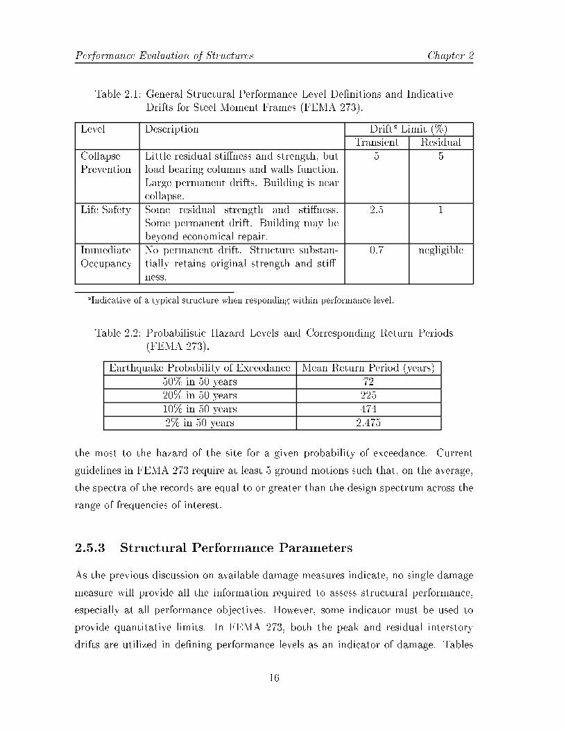
Table 2.1: General Structural Performance Level De�nitions and IndicativeDrifts for Steel Moment Frames (FEMA 273).
Level Description Drifta Limit (%)Transient Residual
CollapsePrevention
Little residual sti�ness and strength, butload bearing columns and walls function.Large permanent drifts. Building is nearcollapse.
5 5
Life Safety Some residual strength and sti�ness.Some permanent drift. Building may bebeyond economical repair.
2.5 1
ImmediateOccupancy
No permanent drift. Structure substan-tially retains original strength and sti�-ness.
0.7 negligible
aIndicative of a typical structure when responding within performance level.
Table 2.2: Probabilistic Hazard Levels and Corresponding Return Periods(FEMA 273).
Earthquake Probability of Exceedance Mean Return Period (years)50% in 50 years 7220% in 50 years 22510% in 50 years 4742% in 50 years 2,475
the most to the hazard of the site for a given probability of exceedance. Current
guidelines in FEMA 273 require at least 5 ground motions such that, on the average,
the spectra of the records are equal to or greater than the design spectrum across the
range of frequencies of interest.
2.5.3 Structural Performance Parameters
As the previous discussion on available damage measures indicate, no single damage
measure will provide all the information required to assess structural performance,
especially at all performance objectives. However, some indicator must be used to
provide quantitative limits. In FEMA 273, both the peak and residual interstory
drifts are utilized in de�ning performance levels as an indicator of damage. Tables
16
Chapter 2 Performance Evaluation of Structures
are provided that contain limiting drift values, for di�erent structural systems, for
the di�erent performance levels. The indicative drift values for steel moment-resisting
frames (SMRF) are shown in Table 2.1. The document emphasizes that these drift
values are indicative of the drifts a structure will experience at that performance
level. They should be used as indicators, and not as design or evaluation limits. For
use in the design and evaluation process, FEMA 273 further provides information on
component level peak deformation values relative to the analysis procedure used for
evaluation.
Peak transient drift serves as an indicator of damage to low strength rigid elements,
such as building cladding and partition walls, and the maximum deformation of the
structural elements. The permanent drift provides a rough indicator of damage to
structural members. Care must be taken in the interpretation of this value, however,
as it may be misleading. For example, a large cyclic loads may result in small residual
drifts, while a half-pulse load of signi�cant smaller amplitude may result in large
residual drifts.
The use of maximum values as an indicator of damage provides preliminary infor-
mation to be used in the evaluation of the structural system. However, the informa-
tion is incomplete, as it does not account for the cumulative damage incurred during
seismic loads. In the following discussions on the performance of the di�erent sys-
tems analyzed, the FEMA 273 values are used to provide an estimate of the expected
structural performance. However, discussions on cumulative damage, as indicated by
dissipated hysteretic energy, and nonstructural damage, as indicated by peak oor
acceleration, are also provided.
17

Chapter 3
Structural Control in Civil
Engineering Structures
3.1 Introduction
The protection of civil structures, including their material contents and human oc-
cupants, is of serious global importance. Such protection may range from reliable
operation and comfort to survivability. Examples of such structures include build-
ings, o�shore rigs, towers, roads, bridges, and pipelines. Events which cause the need
for such protective measures include earthquakes, winds, and waves. Research in this
�eld indicates that control methods will be able to make a genuine contribution to
this problem area.
The common feature of the di�erent proposed approaches is the modi�cation of
the dynamic interaction between the structure and the dynamic loads. The goal of the
modi�cation is to minimize the damage and vibrations throughout the structure. The
result is that well-designed controlled systems display enhanced safety and occupant
comfort.
This chapter provides an overview of the basic ideas and concepts of structural
control as applied to civil engineering structures. Previous work in the area is collected
and reviewed. A discussion of how structural control methods �t within the goals of
performance engineering is then presented.
18

Chapter 3 Structural Control in Civil Engineering Structures
3.1.1 Background and Recent Developments in Structural
Control
Various means of controlling structural vibrations produced by earthquake or wind
have been investigated by the structural engineering community. These means include
modifying rigidities, masses, damping, or shape through the provision of countering
forces. A structure that is designed solely on the basis of strength requirements
does not necessarily ensure that the building will respond dynamically in such a way
that the comfort and safety of the occupants is maintained. For example, a 47-
story building in San Francisco experienced peak accelerations of 0.45g on the top
oor (Housner et al. 1997), resulting in signi�cant nonstructural damage.
The notion of structural control in civil engineering can be traced back to John
Milne, over 100 years ago, who built a small wood house and placed it on bearings
to illustrate how it could be isolated from earthquake vibrations. During the �rst-
half of the twentieth century, development of system theory and its application to
vibration control was driven by the development of the internal combustion engine.
The engine, which was used in both automobiles and aircrafts, produced signi�cant
forces at connection points to the surrounding system. Structural control theory
was applied so as to counteract those forces. During the World War II the concepts
of vibration isolation and absorption were further developed and applied to aircraft
structures (Housner et al. 1997).
The structural engineering community began to seriously investigate the appli-
cation of control techniques in the 1960's. Knowledge has largely been adapted
from both the aerospace and automobile industries, where a signi�cant amount of
research and applications have occurred. In structural engineering, the means of vi-
bration control have taken several forms; for example, the use of base isolation for
low and medium height structures for seismic protection. For taller, more exible
structures, particularly those susceptible to high winds, the addition of supplemental
dampers have been successfully employed. One well-known example where viscoelas-
tic dampers are utilized to control wind-induced vibrations is the World Trade Center
in New York City.
Special considerations distinguish the application of control to civil engineering
structures as opposed to other engineering applications. One such di�erence lies in
19

Structural Control in Civil Engineering Structures Chapter 3
the fact that civil structures are anchored to the ground and so are statically stable.
In contrast, space structures when deployed require active control for stability. Also,
environmental disturbances, such as winds and earthquakes, are highly uncertain with
respect to both their occurrence and intensity. The loads found in most mechanical
applications, however, are fairly well documented.
Since the initial conceptual studies were conducted, the �eld of vibration control
has slowly matured and found application in the civil engineering arena. The U. S.
National Workshop on Structural Control, held at the University of Southern Califor-
nia in 1990, attracted nearly 100 participants from around the globe. By the Tenth
World Conference on Earthquake Engineering in Madrid, Spain in 1992, several tech-
nical sessions were dedicated to topics in structural control. At this conference, the
decision was made to form an international association and hold world conferences
dedicated to structural control. The resulting International Association of Struc-
tural Control (IASC) was formed the following year, with Professor G. Housner as
president. Their e�orts led to the First World Conference in Structural Control in
1994, several workshops and technical sessions at earthquake engineering conferences,
the �rst European Conference in Structural Control, and in 1998 the Second World
Conference in Structural Control in Tokyo.
3.1.2 General Classi�cation of Control Systems
The control of structural systems can be subdivided on the basis of the approach
taken to produce the desired response. The basic classi�cations used in structural
control are de�ned below.
Isolation systems introduce, at the foundation of the structure, a system that
is characterized by increased exibility and high energy absorption capacity. The
increased exibility provided shifts the fundamental period to a range of reduced
energy input from the ground motion. The isolation system's energy dissipation
capacity then further reduces the displacement demands on the superstructure.
Passive control systems do not require external forces. The forces imparted to
the structural system are a function of the response to the excitation. These systems
function by increasing the dissipated energy capacity of the structure and focusing
energy dissipation in specially designed devices.
20

Chapter 3 Structural Control in Civil Engineering Structures
Active controls systems contain external source powers actuators that apply forces
in speci�ed manner. They both add and dissipate energy in the structure. Closed-
loop control uses information about structural response only, measured with physical
sensors. Open-loop control results when control forces are determined only from mea-
sured excitations. Open-closed-loop control uses information from both the structural
response and the external excitation.
A semi-active control system can be considered as a passive device whose proper-
ties can be actively controlled. For example, a uid viscous damper whose damping
constant can be controlled. These systems require power inputs which are signi�cantly
reduced from a fully active system.
The term hybrid control implies the combination of both passive and active control
systems. Generally, a passive device is utilized to control the larger portion of the
response, while the active device is utilized to optimize the response to the given
excitation and maintain the passive system within desired parameters. For example,
a base isolation system could have excessive displacements in the isolation unit that
are then controlled through the use of an active actuator.
3.2 Isolation Systems
A seismic isolation system introduces, at the base of the structure, a system which is
characterized by high exibility and energy absorption capacity. Buckle and Mayes
(1990) identi�ed the basic elements in a practical isolation system as: (1) exibility
to lengthen the period and produce isolation e�ect, (2) energy dissipation capability
to reduce displacement demands to a practical design level, and (3) a means for
providing rigidity under service loads, such as winds
Examples of modern isolation systems include high damping elastomeric bearings,
lead-core rubber bearings, and friction sliding bearings. In hysteretic isolation systems
(high damping rubber bearings, lead-rubber bearings, sliding bearings), high levels
of energy dissipation can lead to out-of-phase, high accelerations in superstructure.
These accelerations, however, are still less than those observed in the uncontrolled
structure (Soong and Constantinou 1994). While high accelerations are undesirable
in the protection of acceleration-sensitive building contents, high levels of hysteretic
damping are bene�cial in protecting the structural system.
21

Structural Control in Civil Engineering Structures Chapter 3
The �rst isolated building in the United States was the Foothill Communities Law
and Justice Center in San Bernadino, CA, which was constructed in 1986. Since that
time, a number of isolated structures, including buildings and bridges, have been
constructed. A survey of these structures is presented in Soong and Constantinou
(1994). The basic properties of elastomeric and sliding bearings are presented in the
following sections.
3.2.1 Elastomeric Bearings
Elastomeric bearings consist of thin layers of natural rubber which are vulcanized
and bonded to steel plates. Rubber has low shear modulus, G, ranging from 0.5-1
MPa at a shear strain of about 50% (Soong and Constantinou 1994). The insertion of
steel plates does not the a�ect shearing capacity, so the e�ective horizontal sti�ness
is given by:
Khz =ArGPtr
(3.1)
where Ar is the bonded rubber area andPtr is the total rubber thickness. The steel
plates are used to reduce the capacity of rubber to bulge in the vertical direction, so
the vertical sti�ness is large.
Elastomeric bearings with low-damping natural rubber have an equivalent viscous
damping in the order of 0.05 or less of critical. They are useful in the isolation of
structures with highly sensitive equipment, where reduction of accelerations is of
primary importance.
Lead-rubber bearings are constructed of low-damping natural rubber with a pre-
drilled center-hole in which a lead core is press-�tted. The lead core deforms in almost
pure shear and, at normal temperatures, yields at low levels of stress. The resulting
behavior is hysteretic curves which are stable over a number of cycles. Furthermore,
due to the recrystalization of the lead at normal temperatures, repeated yielding does
not cause fatigue.
High-damping rubber bearings utilize specially compounded rubber. The resulting
equivalent damping ratios range from 0.10 to 0.15 of critical. They were developed
originally in the United Kingdom and �rst found application in U.S. at the Foothill
22

Chapter 3 Structural Control in Civil Engineering Structures
Communities Center in California (Soong and Constantinou 1994).
3.2.2 Sliding Bearings
Flat isolation bearings limit the transmission of force across the isolation interface.
However, they also require recentering devices, otherwise large permanent displace-
ments result that can accumulate to unacceptable levels (Constantinou et al. 1991).
Constantinou et al. (1993) and Tsoupelas et al. (1994) have investigated various
means of providing the necessary restoring force to these systems. The most practi-
cal is the use of a spherical sliding surface as in the Friction Pendulum System (FPS)
bearings.
R
F
W
θ
u = R sin θ
N
Ff
Figure 3.1: Free-body Diagram for FPS Isolation System
The FPS bearing consists of an articulated slider on a spherical surface, which
is faced with a polished stainless-steel overlay. The restoring force is generated by
the rising of the structure along the spherical surface, while energy is dissipated
by friction. The force needed to produce a displacement in the bearing consists
of a restoring force, due to the rising of the structure along the spherical surface,
and a frictional force along the sliding interface. A free-body diagram of the FPS
23

Structural Control in Civil Engineering Structures Chapter 3
isolation bearing is shown in Figure 3.1. The horizontal and vertical components of
displacement are respectively given by:
u = R sin(�)
v = R(1� cos(�))(3.2)
where R is the radius of curvature of the spherical sliding surface. From equilibrium,
the lateral force, F, is
F = W sin(�) +Ff
cos(�)(3.3)
whereW is the weight carried by the bearing and Ff is the friction force at the sliding
interface.
F =W
R cos(�)u+
Ffcos(�)
(3.4)
For small values of the angle �, Equation (3.4) can be simpli�ed to:
F =W
Ru+ �SW sgn( _u) (3.5)
where � is the friction coeÆcient, and _u is the velocity across the bearing. The FPS
bearings are typically designed for displacement u < 0:2R to minimize the lineariza-
tion error and reduce forces induced in structural columns. Previous analytical and
experimental investigations have demonstrated that these approximations are valid
in the calculation of the system responses for all practical purposes (Zayas et al.
1987; Mokha et al. 1991; Constantinou et al. 1993). If vertical ground motions are
expected to be signi�cant, recent research has shown that more complex models of
the isolation system are required (Llera and Almazan 1998).
The friction force which is generated at the sliding interface depends on the nor-
mal load, bearing pressure, direction and value of sliding velocity, and composition of
the sliding interface. The frictional properties of PTFE (te on) and stainless steel in-
terfaces have been studied by Mokha (1988) and Constantinou (1990). Constantinou
24

Chapter 3 Structural Control in Civil Engineering Structures
proposed that:
�S = fmax � (fmax � fmin) exp�aj _uj (3.6)
where �S is the sliding coeÆcient of friction, _u is the velocity of sliding, fmax is the
coeÆcient of sliding friction at high velocity, fmin is the coeÆcient of sliding friction
at low velocity, and a is a coeÆcient controlling the dependency of friction on sliding
velocity. In general, the parameters fmax, fmin, and a are determined experimentally
depending on bearing pressure, surface roughness, and the composition of PTFE.
Table 3.1 presents the values of these parameters from the tests of Mokha (1988),
where: UF = Un�lled Te on; 15GF = glass-�lled Te on at 15%; 25GF = glass-�lled
Te on at 25%; P = sliding parallel to the direction of the te on lay; T = sliding
perpendicular to direction of the te on lay.
Table 3.1: Frictional Properties of PTFE in Contact with Polished StainlessSteel
Type Pressure Sliding fmax fmin aTe on (MPa) Direction (%) (%) (sec/in)UF 6.9 P 11.93 2.66 2.2UF 13.8 P 8.70 1.75 2.3UF 20.7 P 7.03 1.51 3.7UF 44.9 P 5.72 0.87 4.315GF 6.9 P 14.61 4.01 2.115GF 13.8 P 10.08 4.28 1.415GF 20.7 P 8.40 4.32 1.315GF 44.9 P 5.27 2.15 2.225GF 6.9 P 13.20 5.54 1.425GF 13.8 P 11.20 4.87 1.425GF 20.7 P 9.60 4.40 1.525GF 44.9 P 5.89 3.19 1.8UF 6.9 T 14.20 2.39 3.0UF 13.8 T 10.50 1.72 4.4UF 20.7 T 8.20 2.90 1.5UF 44.9 T 5.50 1.11 3.2
Since the force is proportional to the weight carried by the bearings, the resultant
25

Structural Control in Civil Engineering Structures Chapter 3
force of all bearings always develops at the center of mass of the structure, therefore
eliminating eccentricities even in the case of uneven mass distribution. Another useful
property of this system is that the period of isolation for the system is independent
of the mass of the structure. In Equation (3.5), the sti�ness of the bearing is given
by the quantity W=R. Therefore, the period of isolation is given by:
T = 2�
�W
Kg
�1=2
= 2�
�R
g
�1=2
(3.7)
Several structures have been built in recent years which utilize FPS isolators or
similar devices. The U.S. Court of Appeals in San Francisco is one recent and well
documented example (Mokha et al. 1996). This structure was damaged in the 1989
Loma Prieta earthquake and was retro�tted using 256 FPS isolators. The structure
has a oor area of 31500 square meters and a weight of 55000 metric tons.
3.3 Passive Control Systems
Passive Control Systems increase the hysteretic energy dissipation capacity of the
structure. By increasing the amount of energy dissipated through hysteretic behavior
of passive devices, the amount of energy needed to be dissipated through strain de-
formation of the structure is reduced. Energy dissipation is concentrated in specially
designed and detailed areas and away from critical load bearing members. Passive de-
vices have long been used to control response to wind loads. The towers in the World
Trade Center and Seattle's Columbia Sea�rst Center both utilize passive viscoelas-
tic dampers to control wind induced vibrations (Mahmoodi et al. 1987). Recently,
passive systems have also been found to be an eÆcient means of controlling seismic
excitations (Lin et al. 1991; Cherry and Filiatrault 1993).
Aiken et al. (1993) investigated passive energy dissipation systems for earthquake-
resistant design. They categorize passive energy dissipation devices into two broad
categories of rate-dependent or rate-independent on the basis of whether the hysteretic
characteristics of the device are dependent on the rate of loading. Examples of rate-
dependent devices include viscous and viscoelastic systems; rate-independent devices
include friction-slip, steel yielding and shape-memory systems.
26

Chapter 3 Structural Control in Civil Engineering Structures
The two most commonly used and researched devices are the viscoelastic and the
friction-slip systems. A major di�erence between these two devices is the maximum
force that each will develop during an earthquake (Hanson 1993). Viscoelastic devices
produce maximum forces which are proportional to the maximum displacements and
velocities across the the device. In contrast, friction-slip devices produce maximum
forces equal to the design friction force plus strain hardening. As a result, the maxi-
mum force experienced by the passive control device can be more readily controlled
in the friction devices.
3.3.1 Viscous and Viscoelastic Dampers
Though viscoelastic dampers have long been used in response control under wind
loads, their use in seismic response control has been investigated only in recent years.
Both analytical and experimental investigations have indicated that signi�cant reduc-
tions in structural response can be achieved by the use of viscoelastic dampers (Aiken
and Kelly 1990; Lin et al. 1991; Zhang et al. 1989). However, experimental stud-
ies have also shown that, while e�ective in controlling structural response, achieving
maximum eÆciency in their design requires careful consideration of several key fac-
tors, such as excitation frequencies and environmental temperature (Aiken and Kelly
1990).
Some viscoelastic damping is present in all building structures, and their e�ects
on the dynamic response of the structure has long been recognized and accepted.
Typical values of damping utilized in design range from 2% to 5%, which account
for the inelastic behavior in the structural members. By increasing the percentage
of critical damping in the system, the dynamic ampli�cation factor is correspond-
ingly reduced in the range of the system's natural frequency. Outside that frequency
range, an increase in the viscous damping will not signi�cantly impact the building
response (Hanson 1993). The behavior of the viscoelastic material itself is not con-
stant. Mahmoodi (1969) conducted experimental analysis on the viscoelastic material
and found that their material behavior is strongly in uenced by its shear modulus,
the shear storage modulus, and the material loss factor. These material properties,
in turn, are dependent on frequency, temperature, and deformation strain level.
27
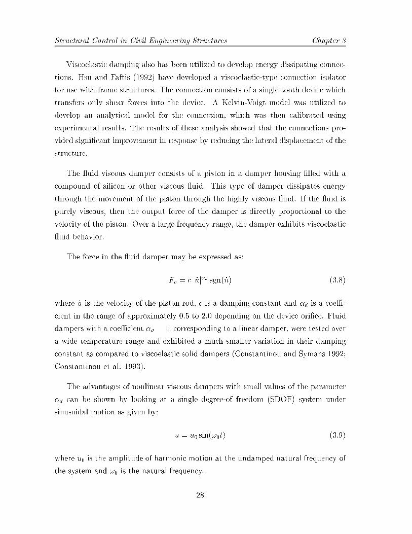
Structural Control in Civil Engineering Structures Chapter 3
Viscoelastic damping also has been utilized to develop energy dissipating connec-
tions. Hsu and Faftis (1992) have developed a viscoelastic-type connection isolator
for use with frame structures. The connection consists of a single tooth device which
transfers only shear forces into the device. A Kelvin-Voigt model was utilized to
develop an analytical model for the connection, which was then calibrated using
experimental results. The results of these analysis showed that the connections pro-
vided signi�cant improvement in response by reducing the lateral displacement of the
structure.
The uid viscous damper consists of a piston in a damper housing �lled with a
compound of silicon or other viscous uid. This type of damper dissipates energy
through the movement of the piston through the highly viscous uid. If the uid is
purely viscous, then the output force of the damper is directly proportional to the
velocity of the piston. Over a large frequency range, the damper exhibits viscoelastic
uid behavior.
The force in the uid damper may be expressed as:
Fv = c j _uj�d sgn( _u) (3.8)
where _u is the velocity of the piston rod, c is a damping constant and �d is a coeÆ-
cient in the range of approximately 0.5 to 2.0 depending on the device ori�ce. Fluid
dampers with a coeÆcient �d = 1, corresponding to a linear damper, were tested over
a wide temperature range and exhibited a much smaller variation in their damping
constant as compared to viscoelastic solid dampers (Constantinou and Symans 1992;
Constantinou et al. 1993).
The advantages of nonlinear viscous dampers with small values of the parameter
�d can be shown by looking at a single degree-of freedom (SDOF) system under
sinusoidal motion as given by:
u = u0 sin(!0t) (3.9)
where u0 is the amplitude of harmonic motion at the undamped natural frequency of
the system and !0 is the natural frequency.
28

Chapter 3 Structural Control in Civil Engineering Structures
The damping ratio for an SDOF system with a damper with characteristics de-
scribed in Equation (3.8) is de�ned by (Constantinou 1994):
� =Ed
2�Ku20(3.10)
where Ed is the dissipated energy in one cycle of loading, and K is the sti�ness of the
system. By substituting for the dissipated energy, the resulting expression becomes:
� =1
2�Ku20
Z T
0
Fv _udt =21+�dcu�d�10 !�d�20
�m� �2(1 + �d
2)
�(2 + �d)(3.11)
where T = 2�=!0, m is the inertial mass, and � is the gamma function.
For dampers with �d > 1, the damping ratio decreases with increasing amplitude
of motion, making them undesirable for vibration control problems. For dampers with
�d < 1, the damping ratio increases with increasing amplitude of motion, whereas for
linear dampers the damping ratio is independent of the amplitude of motion. One
advantage of dampers with �d < 1 is that the force tends to atten out at higher
velocities (Constantinou 1994), providing an upper-bound on the expected force
levels.
Taylor Devices, Inc. is one company that is widely involved in developing uid
damping devices for seismic protection. These devices are rated and proof tested
to a minimum burst pressure of 20,000 psi, per U. S. government standards. The
operating uid is inert silicon, with an operating temperature range from -40Æ to 160Æ
F. Table 3.2 lists the properties of a few of the high capacity linear uid viscous
dampers available from Taylor Devices, Inc.
Most early studies into the e�ect of viscous dampers on structural response treated
the structure as SDOF systems (Lin et al. 1991). Zhang and Soong (1992) have pro-
posed a sequential procedure for the optimal placement of the dampers. The location
of the dampers were determined based on the concept of degree of controllability.
Dampers were placed where the response of the uncontrolled structure is the largest.
The dampers were tested at several di�erent ambient temperatures. Though the per-
formance of the damper degraded at higher temperatures, it still contributed to the
overall damping of the structure for all temperature values tested. Recently, Shen and
29

Structural Control in Civil Engineering Structures Chapter 3
Table 3.2: High Capacity Fluid Viscous Dampers from Taylor Devices, Inc.
Maximum Force Extended Length Bearing Width(kips) (inches) (inches)100 131 7.5200 132 9.0300 138 11.5600 155 16.01000 166 23.02000 180 26.0
Soong (1996) have proposed a simple design procedure based on the the minimiza-
tion of the Park and Ang damage index, described in Section 2.4.3. They propose
a transformation of an MDOF system to an equivalent SDOF model in the inelastic
range so that the damage function can be applied.
3.3.2 Friction-Slip Dampers
Friction-slip devices have also been studied as a means of controlling the seismic
response of buildings. These devices contain specially designed surfaces that are
designed to slip past one another at a predetermined load value, called the slip load.
During severe excitations, the device slips before any main structural members have
yielded. Until the load across the device reaches the slip load, no energy dissipation
occurs. Since the behavior of these devices rely on nonlinear behavior, a nonlinear
dynamic response calculation should be performed to verify that the desired building
response was achieved (Hanson 1993).
Friction devices have demonstrated excellent energy dissipating characteristics
(Aiken et al. 1993; Filiatrault 1990; Grigorian et al. 1992). Their hysteretic behavior
is regular and repeatable, with a nearly perfect rectangular shape to the hysteretic
curve. The force displacement response has been shown to be basically independent
of loading frequency, amplitude, number of loading cycles, and temperature (Aiken,
Nims, Whittaker, and Kelly 1993).
One type of friction device was developed by Pall in 1982, called a Pall Friction
Device (Filiatrault 1990; Cherry and Filiatrault 1993). This system consists of
30

Chapter 3 Structural Control in Civil Engineering Structures
a mechanism containing brake lining pads introduced at the intersection of frame
crossings. In order to be fully e�ective, the device must slip in both compression and
tension, otherwise energy will be dissipated only in the �rst few cycles. If the bracing
elements are designed not to buckle in compression, then a simple friction joint would
suÆce. However, designing braces to this requirement is often not economical. The
Pall device causes the friction design to slip in both tension and compression by
simultaneously connecting the friction mechanism at the intersection of the frame
cross-braces. The element sliding in tension then causes the other element to slip
back to its original position, so it can immediately absorb energy when the cycle
reverses. A. Filiatrault and S. Cherry (1987) have developed a simpli�ed analysis
technique for these devices.
Another type of friction device is a Slotted Bolted Connection (SBC's). SBC's
have recently been studied as simple and inexpensive friction-slip devices (Grigo-
rian, Yang, and Popov 1992; Grigorian and Popov 1994). SBC's are modi�ed bolted
connections designed to dissipate energy during rectilinear tension and compression
loading cycles. The devices were �rst tested on an MTS loading frame and tested
under displacement control (Grigorian, Yang, and Popov 1992). SBC's which include
a shim-like brass insert plate show almost no variation in the slip force magnitude.
These devices can be approximated as an elastic-perfectly-plastic connections. They
were also tested as part of a braced structural frame (Grigorian and Popov 1994).
Both analytical and experimental results were presented, showing that properly de-
signed SBC's incorporated into structural systems are highly e�ective at dissipating
seismic energy.
3.4 Active Control
In comparison with passive systems of the type described in previous sections, the
research and development of active structural control strategies is more recent. The
advantages that typically cited for active control systems are: (1) enhanced e�ec-
tiveness in motion control, limited only by capacity of the system, (2) applicability
to multi-hazard applications, and (3) selectivity of control objectives. Active control
systems are used to control the response of structures to internal or external exci-
tation, such as machinery, wind, or earthquakes. However, the addition of purely
31

Structural Control in Civil Engineering Structures Chapter 3
active control carries a risk of possible destabilization of the structure. Given that
civil engineering structures are statically stable, as they are attached to the ground,
active control solutions have been slower to be accepted in civil engineering practice
as compared to passive control solutions.
3.4.1 Basic Principles
Active control is branch of engineering concerned with the design of systems that
are able to act so as to force a system to behave according to some prescribed spec-
i�cations. The behavior of the system is described by means of a dynamic system
characterized by state variables. The relationship between the system and the ex-
ternal environment is described in terms of input variables, which represent external
actions on the system, and output variables, which are measurable responses on the
system. As mentioned previously, two basic controller arrangements are: open-loop
and closed-loop. In open-loop control, the controller manipulates the system by try-
ing to drive output to a speci�ed behavior without using information regarding the
output. This type of control su�ers by not allowing it to compensate for errors due to
perturbations in either the input, from unknown or unmeasured disturbances, or sys-
tem parameters. In contrast, closed-loop control uses information about the system
response as feedback information. The basic elements found in a closed-loop control
system are shown in Figure 3.2.
The following naming conventions are used to describe the combination of the
structural system and active control components. An actuator architecture or actuator
system refers to the physical actuator system, with their corresponding location and
capacities. The sensor system is the set of sensors, their locations, and �ltering
qualities. Sensors can be used to measure both the input and output response. Closing
the loop is the controller, which is the system that processes the sensor measurements
and determines how the control system should respond by sending the appropriate
signals to the actuators. The control algorithm provides the mathematical theory
within which the controller is formulated.
Studies into active control of civil engineering have ourished since its introduction
to the �eld by Yao (1972). Topics of research conducted to date include H2 and H1
control (B. F. Spencer and Sain 1997; Suhardjo et al. 1992; B. F. Spencer et al. 1994),
32

Chapter 3 Structural Control in Civil Engineering Structures
Structure SensorsActuators
Controller
Excitation
Output
Control Signal
Figure 3.2: Basic Elements of a Closed-Loop Active Control
sliding mode control (Nonami et al. 1994; Yang et al. 1995), e�ects of actuator satura-
tion on control (Chase and Smith 1996), reliability-based control (B.F. Spencer et al.
1992; R.V. Field et al. 1996; R. V. Field and Bergman 1997), fuzzy control (Nagara-
jaiah 1994), neural control (Venini and Wen 1994; Ghaboussi and Joghataie 1995),
nonlinear control (Agrawal and Yang 1996), modelling issues (Smith and Schemmann
1996; Dyke et al. 1995), and benchmark studies (B.F. Spencer et al. 1997). Ref-
erences to the current state-of-the-art in active control can be found in Spencer et
al. (1997) and Housner et al. (1997).
Common actuator systems found in civil engineering applications include the ac-
tive mass driver (AMD) and the active tendon brace (ATB) systems. The AMD
actuation system is composed of a small, relative to the structure, additional mass,
that is activated by servo-hydraulic actuators which connects the mass to the struc-
ture. The system is typically located near the top of the structure so as to be most
e�ective at controlling the �rst mode of the structure. The ATB actuation system
uses a tendon/pulley system to transmit the force generated by the hydraulic actu-
ator to the structure. These actuators can be placed throughout the height of the
structure and can be useful in controlling various vibrational modes.
Consider a linear structure modeled by an n-dof shear building model, where the
matrix equation of motion can be written as:
M�x(t) +C_x(t) +Kx(t) = Gu(t) + Jf(t) (3.12)
33
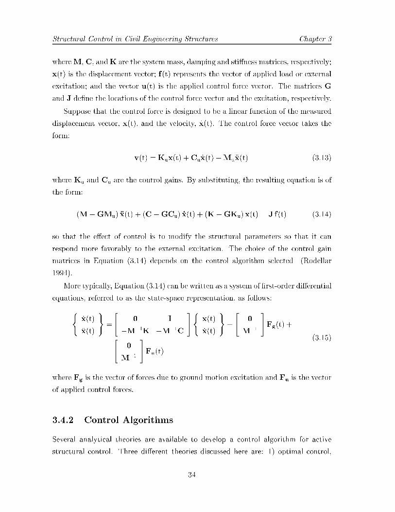
Structural Control in Civil Engineering Structures Chapter 3
whereM, C, andK are the system mass, damping and sti�ness matrices, respectively;
x(t) is the displacement vector; f(t) represents the vector of applied load or external
excitation; and the vector u(t) is the applied control force vector. The matrices G
and J de�ne the locations of the control force vector and the excitation, respectively.
Suppose that the control force is designed to be a linear function of the measured
displacement vector, x(t), and the velocity, _x(t). The control force vector takes the
form:
v(t) = Kux(t) +Cu _x(t) +Mu�x(t) (3.13)
where Ku and Cu are the control gains. By substituting, the resulting equation is of
the form:
(M�GMu) �x(t) + (C�GCu) _x(t) + (K�GKu)x(t) = J f(t) (3.14)
so that the e�ect of control is to modify the structural parameters so that it can
respond more favorably to the external excitation. The choice of the control gain
matrices in Equation (3.14) depends on the control algorithm selected (Rodellar
1994).
More typically, Equation (3.14) can be written as a system of �rst-order di�erential
equations, referred to as the state-space representation, as follows:
(_x(t)
�x(t)
)=
"0 I
�M�1K �M�1C
#(x(t)
_x(t)
)+
"0
M�1
#Fg(t) +"
0
M�1
#Fu(t)
(3.15)
where Fg is the vector of forces due to ground motion excitation and Fu is the vector
of applied control forces.
3.4.2 Control Algorithms
Several analytical theories are available to develop a control algorithm for active
structural control. Three di�erent theories discussed here are: 1) optimal control,
34

Chapter 3 Structural Control in Civil Engineering Structures
2) stochastic control, and 3) robust control. The optimal control design involves
minimizing or maximizing a performance measure, or cost function. One example for
linear systems is the minimization of a quadratic cost function, such as:
J =1
2x(tf)
TSx(tf) +
1
2
Z tf
t0
fx(t)T Qx(t) + u(t)T Ru(t)gdt (3.16)
where S, Q, R, are weighting matrices x(t) is the state of the system and u(t) is the
control vector. Though the cost function itself has no physical meaning, it is used
to weight two variables that do have a physical signi�cance. The matrix S penalizes
the state vector at the end of the analysis. By manipulating the relative values
of Q and R, a controller can be designed that compromises between maintaining
the state close to the origin while not allowing the control e�ort to be excessive.
The advantage of linear quadratic (LQ) control is its simplicity and the fact that it
results in a linear controller; however, these controllers have limited success in seismic
applications, largely due to their inability to account for uncertainties in the structural
system (Housner et al. 1997; Skelton and Shi 1996; Soong and Constantinou 1994).
The use of stochastic control encompasses a number of functions. Among these
are (Housner et al. 1997):
� The determination of control policy for a dynamic system subject to random
vibrations so as to achieve some speci�ed objective
� The use of incomplete or noisy information in the estimation of the states of
the dynamic system.
� Ability to assess the robustness of a control system with respect to the uncer-
tainty in the structure and control parameters and system inputs.
The time-optimal control problem considered requires the determination of a control
vector, u(t), that minimizes a scalar cost function of the form:
J = �(x(tf) ;w(tf) ;p(tf) ; tf) +
Z tf
t0
L(x(t) ;u(t) ;w(t) ;p(t) ; t) dt (3.17)
where x(t) is the n-dimensional state vector; u(t) is the control vector; w(t) is a
vector of disturbances; p(t) is a vector of system parameters; �(�) expresses the
terminal constraint; and L(�) is the Lagrangian. Though the above expression �nds
35

Structural Control in Civil Engineering Structures Chapter 3
many applications in structural engineering, the solution of the control problem is not
easily determined. So as to simplify the problem, the cost function is generally given
as the expected value of the expression of Equation (3.17). Also, the disturbances
and sensor noise are assumed to be small and additive, and the parameters and
initial conditions of the system are assumed to be random variables. However, the
determination of the optimal control inputs requires knowledge of the state vectors,
implying a recursive nonlinear estimation and design procedure, limiting its general
application to civil engineering structures (Housner et al. 1997).
Robust control focuses on the issues of system performance in the presence of
uncertainty in both parameter and system inputs. LQ theory, which is discussed
brie y above, cannot explicitly accommodate uncertainties in the structure parame-
ters. This need led to the development of H1 problem, principally in the frequency
domain. The objective of H1 control is to design a controller such that the in�nity
norm of the transfer function from input excitations, w(t), to controlled responses,
y(t) is minimized. Mathematically, this expression is given by:
k Tyw k1= supw(t)
k y(t) k2k w(t) k2 � (3.18)
where Tyw is de�ned as the transfer function between w(t) and y(t), sup is the
supremum over all w(t), and is a positive, scalar attenuation constant, which is
speci�ed by the designer. k y(t) k2 indicates the 2-norm of y(t) and is given by
k y(t) k2= (y1(t)2 + y2(t)
2 + � � �+ yq(t)2)
1
2 , where q is the number of sensor measure-
ments. In general, this transfer function contains measures of nominal performance
and stability robustness. An important characteristic of this problem is that the H1
norm gives a measure of the worst case response of the system over an entire class
of input disturbances. Application of H1 control theory to civil engineering struc-
tures has been investigated by several researchers, and a good summary can be found
in Housner et al. (1997).
36

Chapter 3 Structural Control in Civil Engineering Structures
3.5 Role of Structural Control in Performance-Based
Engineering
Structural control provides an extra mechanism to improve structural performance.
For maximum e�ectiveness, minimal control e�ort would be required to achieve the
desired performance goals. In active control, this control e�ort is measured in terms of
the energy and forces required of the actuation system. Attempting to apply very large
control forces may not be physically realizable. Under severe seismic loads, meeting
the desired performance objective may be unattainable with a given controller design
and architecture. In such cases, a di�erent control solution should be investigated.
Extensive work in the �eld of passive energy dissipation have resulted in tenta-
tive requirements for the design and implementation of passive energy dissipation
devices in the United States. The Energy Dissipation Working Group of the Base
Isolation Subcommittee of the Structural Engineers Association of Northern Califor-
nia (SEAONC) has developed a document addressing these tentative requirements,
which provides design guidelines applicable to a wide variety of systems (Whittaker
1992; Whittaker 1993). The general philosophy is to con�ne inelastic deformation to
the energy dissipators, while the main structure remains elastic for the design basis
earthquake.
Recent guidelines (BSSC 1997; BSSC 1998) prepared by the Building Seismic
Safety Council (BSSC) for the Federal Emergency Management Agency (FEMA)
specify provisions which are similar to those developed by SEAONC in both scope
and philosophy. Simpli�ed design procedures are available for both the bearing system
and superstructure depending on the isolation approach. For new buildings, the un-
derlying design philosophy for base isolation systems has two performance objectives.
The primary performance objective is speci�ed for the �xed-base structure, which is
the protection of life-safety for major earthquake. The secondary performance objec-
tive provides damage reduction for the isolated system. For rehabilitation of existing
buildings, the performance objectives may be less stringent depending on the owner's
requirements. If the current structure does not adequately provide for protection of
life-safety, the primary goal of the application of an isolation system would be that
target.
37

Structural Control in Civil Engineering Structures Chapter 3
Passive energy dissipation systems are also speci�cally addressed in in the design
guidelines. For applications in new buildings, the guidelines are only general in na-
ture. They state that the design of the system shall be based on \rational methods of
analysis, using the most appropriate analysis methods." For the rehabilitation of ex-
isting structures, speci�c guidelines are given concerning the modeling of the dampers
and structure, allowable analysis procedures, and the design and construction review.
Current guidelines allow response spectrum analysis for rate-dependent devices, such
as viscous dampers, as long as the remaining structure remains elastic. For all other
systems, such as friction dampers and inelastic systems, a nonlinear dynamic analysis
must be used. As the passive energy dissipation technology is still relatively new, a
conservative approach is taken. For example, an independent review panel must be
formed to conduct a review of any design involving additional passive dampers. Also,
all devices must be tested to shown that they meet design requirements. Though
speci�c performance-based guidelines have not been put forth, a reasonable assump-
tion is that they will be similar to those for base isolation systems. For example, the
primary objective would be the protection of life-safety while the secondary perfor-
mance objective would provide for damage reduction when compared to the initial
structural system.
Active control, which is the newest vibration control technology used in civil
engineering applications, is only brie y addressed in code provisions. The recent
guidelines indicate that these systems may be considered, though the design must be
reviewed by independent review panel, enpaneled by the owner prior to the prelimi-
nary design phase, and fully tested.
Incorporation of the control design process within the overall design process is
illustrated in Figure 3.3. The left side of these �gures represents the design process
for the structure based on the concept of performance-based design. Once the exci-
tation(s) are chosen and the initial structural design is developed based on collapse
prevention criteria, controllers can be used to help meet the performance criteria
associated with minimizing damage. An important consideration is that the uncon-
trolled structural response not compromise life safety; therefore, controllers are not
incorporated until minimal requirements are met.
Referring to Figure 3.3, the shaded region on the right represents the controller
design process. A controller can be designed for the original structure, which together
38
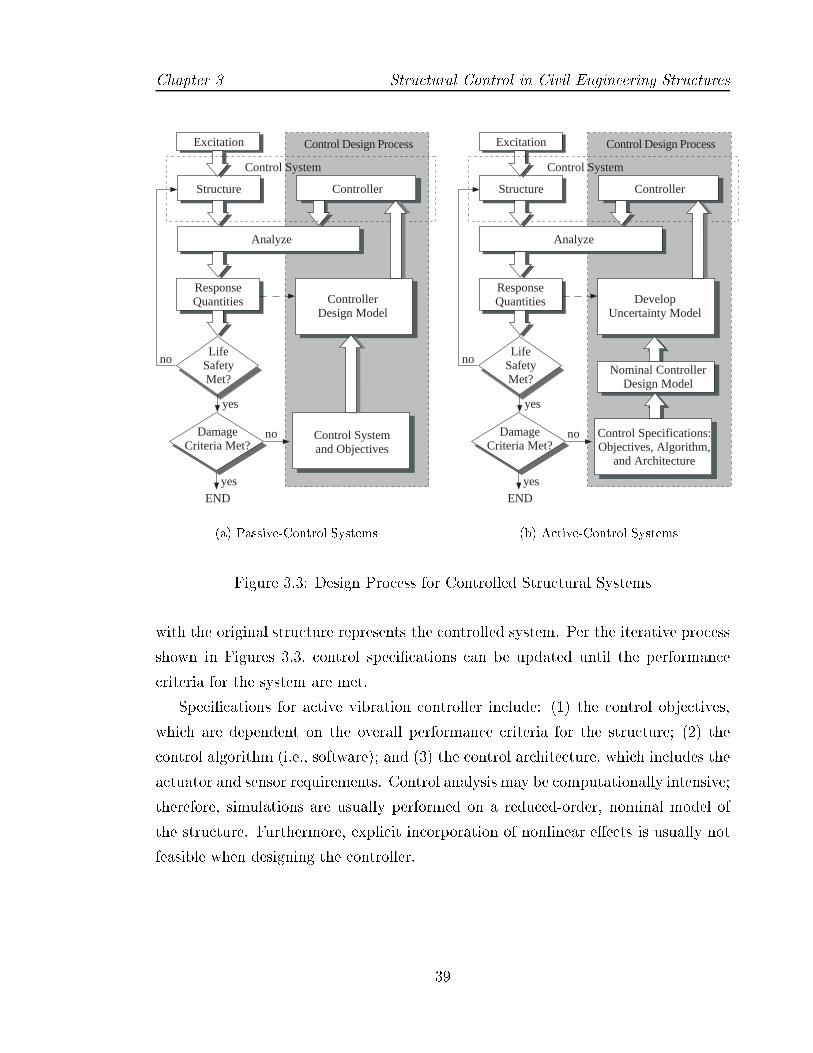
Chapter 3 Structural Control in Civil Engineering Structures
Structure
ResponseQuantities
LifeSafetyMet?
Analyze
DamageCriteria Met?
Controller
Excitation
ControllerDesign Model
Control Systemand Objectives
Control System
Control Design Process
yes
no
yes
no
END
(a) Passive-Control Systems
Structure
ResponseQuantities
LifeSafetyMet?
Analyze
DamageCriteria Met?
Controller
Excitation
DevelopUncertainty Model
Nominal ControllerDesign Model
Control Specifications:Objectives, Algorithm,
and Architecture
Control System
Control Design Process
yes
no
yes
no
END
(b) Active-Control Systems
Figure 3.3: Design Process for Controlled Structural Systems
with the original structure represents the controlled system. Per the iterative process
shown in Figures 3.3, control speci�cations can be updated until the performance
criteria for the system are met.
Speci�cations for active vibration controller include: (1) the control objectives,
which are dependent on the overall performance criteria for the structure; (2) the
control algorithm (i.e., software); and (3) the control architecture, which includes the
actuator and sensor requirements. Control analysis may be computationally intensive;
therefore, simulations are usually performed on a reduced-order, nominal model of
the structure. Furthermore, explicit incorporation of nonlinear e�ects is usually not
feasible when designing the controller.
39

Chapter 4
Description of Case Studies
4.1 Objective of Simulations
The objective of the research presented here is to evaluate the role of structural
control technology in enhancing the overall structural performance under seismic
excitations. This study focuses on steel moment resisting frames, and three types of
possible controllers: (1) base isolation system (passive); (2) viscous brace dampers
(passive); (3) and active tendon braces. Two structures are selected from the SAC
Phase II project: the three story system and the nine story system designed for the
Los Angeles region. Simulations of these systems, both controlled and uncontrolled,
are prepared using the three suites of earthquake records, also from the SAC Phase II
project, representing three return di�erent periods. Several controllers are developed
for each structure and the performance is judged based on the interstory demands
and dissipated hysteretic energy.
This investigation has the following speci�c objectives: (1) To evaluate the ef-
fect of the various controller architectures on seismic demands as described through
performance-based design criteria; (2) To evaluate the sensitivity of the structure-
controller performance to variations of the control parameters, load levels and struc-
tural modeling techniques; (3) To compare the bene�ts of the controllers in both a
deterministic and probabilistic format.
This chapter provides a description of the two structures that are analyzed and
the ground motions utilized for seismic demand calculations. Three di�erent types
of control systems are then selected for implementation with these structures. The
40

Chapter 4 Description of Case Studies
reasoning behind the selection of these systems and the basic design philosophy of
each one is then presented.
4.2 Description of Structures
The structures analyzed are two steel moment-resisting frame buildings (SMRF), one
3-stories and the second 9-stories tall, designed as part of the SAC steel project for the
Los Angeles area. These buildings conform to local code requirements. All buildings
are oÆce buildings designed for gravity, wind, and seismic loads, with a basic live
load of 2.4 kPa (50 psf). The structural system for all buildings consists of steel
perimeter moment frames and interior gravity frames with shear connections. All
columns in the perimeter frame that are part of the lateral force-resisting system
bend about the strong axis. The nominal yield strength of beams is 36 ksi (248.0
MPa) and the nominal yield strength of the columns is 50 ksi (344.5 MPa). However,
the expected strength of the material is very di�erent from the nominal values used
in design (SPPC 1994). So the expected yield strength used for analysis is 49.2 ksi
for beams and 57.6 ksi for columns. The design of the moment frames in the two
orthogonal directions was found to be either identical or very similar, thus only one
direction was chosen for analysis. The typical di�erence in the two directions lies
in the orientation of the gravity beams and sub-beams, which are oriented in the
North-South direction. As a result, only the frames in the North-South direction are
analyzed.
The North-South frame of the 3-story structure has three fully moment-resisting
bays and one simply-connected bay, as shown in Figure 4.2. The columns are �xed at
the base and run the full height of the structure. The dimensions shown in Figure 4.2
are centerline dimensions, and the section sizes are listed next to each corresponding
member.
The North-South frame of the 9-story structure has four fully moment-resisting
bays and one partially moment-resisting bay, as shown in Figure 4.2. The simple
shear connection in the partial moment-resisting bay occurs as a result to avoid bi-
axial bending in the corner columns. One basement level is also present, which is
horizontally restrained at the ground level. The columns are pinned at the base of
the structure and spliced at every other story, indicated by the parallel horizontal lines
41

Description of Case Studies Chapter 4
3rd Floor
2nd Floor
1st Floor
Ground
W24x68 W24x68 W24x68 W21x44
W21x44
W21x44
W30x116 W30x116W30x116
W33x118 W33x118 W33x118
30' - 0'' 30' - 0'' 30' - 0'' 30' - 0''
Figure 4.1: 3-Story Structure: North-South Moment-Resisting Frame
Table 4.1: Column Sections for 9-Story Structure - North-South Frame
Limiting Floor Levels Moment Frame SectionsLower Upper Interior Exterior
-1 1/2 W 14x370 W 14x5001/2 3/4 W 14x370 W 14x4553/4 5/6 W 14x283 W 14x3705/6 7/8 W 14x257 W 14x2837/8 Roof W 14x233 W 14x257
across the columns, with the splice location six feet above the oor. The dimensions
shown in Figure 4.2 are centerline dimensions, and the section sizes for beams are
listed next to each corresponding member. Sections for column members are listed
in Table 4.1.
4.3 Earthquakes
Performance based design approaches are now being used to develop the next genera-
tion of buildings codes (e.g. SEAOC Vision 2000 (SEAOC 1995); SAC Steel Building
Project; FEMA-273 (BSSC 1997). The probabilistic ground motion response spectral
maps recently developed by the USGS provide a �rst-order, non site-speci�c estimate
42
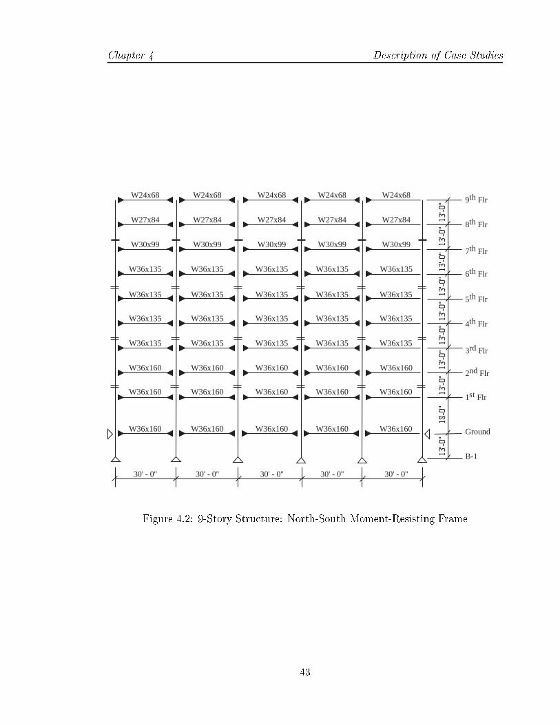
Chapter 4 Description of Case Studies
W24x68 W24x68 W24x68 W24x68 W24x68
W27x84 W27x84 W27x84 W27x84 W27x84
W30x99 W30x99 W30x99 W30x99 W30x99
W36x135
W36x160
9th Flr
8th Flr
7th Flr
6th Flr
5th Flr
4th Flr
3rd Flr
2nd Flr
1st Flr
Ground
B-1
W36x135 W36x135 W36x135 W36x135
W36x135 W36x135 W36x135 W36x135 W36x135
W36x135 W36x135 W36x135 W36x135 W36x135
W36x135 W36x135 W36x135 W36x135 W36x135
W36x160 W36x160 W36x160 W36x160
W36x160 W36x160 W36x160 W36x160 W36x160
W36x160 W36x160 W36x160 W36x160 W36x160
30' - 0'' 30' - 0'' 30' - 0'' 30' - 0'' 30' - 0''
Figure 4.2: 9-Story Structure: North-South Moment-Resisting Frame
43
Description of Case Studies Chapter 4
of the response spectra for use in performance-based design. However, the imple-
mentation of performance-based design requires more detailed speci�cation of input
ground motions than do conventional codes. In particular, many of the methods be-
ing used in the design and analysis of buildings for performance-based design require
ground motion time history inputs.
Suites of ten time histories were generated by Sommerville (1997) to represent
ground motions having probabilities of exceedance of 50% in 50 years, 10% in 50 years,
and 10% in 250 years in the Los Angeles region. These sets of ground motions are
referred to as the 50 in 50 Set, 10 in 50 Set, and 2 in 50 Set, respectively, throughout
this study. The time histories have magnitude-distance pairs that are compatible
with the deaggregation of the probabilistic seismic hazard. Individual time histories
were scaled so that their response spectra are compatible with the spectral ordinates
from the 1996 USGS probabilistic ground motion maps, adjusted for site conditions
from soft rock to sti� soil (from SB/SC boundary to SD), in the period range of 0.3
to 4 seconds. A single scaling factor was found for each time history that minimized
the squared error between the target spectrum and the average response spectrum of
the two horizontal components of the time history assuming lognormal distribution
of amplitudes. The weights used were 0.1, 0.3, 0.3, and 0.3 for periods of 0.3, 1, 2,
and 4 seconds respectively. The scale factor was then applied to all components of
the time history.
The time histories for the 50 in 50 Set are all derived from recordings of crustal
earthquakes on sti� soil (category SD). The time histories are derived from earth-
quakes in the magnitude range 5.7 to 7.7, and the distance range of about 5 to 100
km. With the exception of the Downey recording of the 1987 Whittier Narrows earth-
quake, which was scaled up by a factor of about 3.6, none of the recordings required
scaling by more than a factor of 3.
The time histories for the 10 in 50 Set are all derived from recordings of crustal
earthquakes on sti� soil (category SD). Most of the recorded time histories were
scaled up by factors between 1 and 3 to match the target values. Two recordings
of the magnitude 7.3 Landers earthquake of 1992 at distances of about 40 km are
included to represent large earthquakes on the San Andreas fault at a comparable
distance from Los Angeles. The other eight time histories are near-fault recordings
of strike-slip, oblique and thrust earthquakes in the magnitude range 6 to 7.
44

Chapter 4 Description of Case Studies
For the 2 in 50 Set, all of the time histories are from near-fault recordings or
simulations, and the scale factors required to match the response spectra to the
target spectra are relatively close to unity. The recorded time histories are from
the 1974 Tabas, 1989 Loma Prieta, 1994 Northridge and 1995 Kobe earthquakes.
The simulated time histories are for magnitude 7.1 earthquakes on the Palos Verdes
fault (a strike-slip fault), and on the Elysian Park fault (a blind thrust fault). The
simulated time histories were generated using di�erent methods for the short-period
and the long-period portions of the spectral acceleration curve. The results from
these two methods were then merged near a period of 1 second. As a result, results
for structures in this period range for these records may be questionable.
0 0.5 1 1.5 2 2.5 3 3.5 4 4.5 50
0.5
1
1.5
2
2.5
3
Mean Elastic Spectral Acceleration LA Record Sets, ξ = 2%
Period (seconds)
Acc
eler
atio
n (g
)
50/50 Set10/50 Set2/50 Set
Figure 4.3: Mean Elastic Spectral Acceleration for Ground Motion Sets
The resulting mean spectral acceleration for all three ground motion sets are shown
in Figure 4.3. An important note regarding the earthquake sets is that they should be
used only as a set, and not individually or as small sub-sets as representative of the
probability levels speci�ed. At any particular period the median spectral acceleration
of the set may match the target value reasonably well; however, any individual record
may have a value quite di�erent than the expected target spectral acceleration. A
45

Description of Case Studies Chapter 4
plot showing a measure of the dispersion for the spectral acceleration within each
ground motion set is given in Figure 4.4.
0 0.5 1 1.5 2 2.5 3 3.5 4 4.5 50
0.1
0.2
0.3
0.4
0.5
0.6
0.7
0.8
Measure of Dispersion: Elastic Spectral Acceleration LA Earthquake Sets: ξ = 2%
Period (seconds)
Sta
ndar
d D
evia
tion
of L
n(S a)
2 in 50 Set
10 in 50 Set
50 in 50 Set
Figure 4.4: Dispersion of the Elastic Spectral Acceleration for Ground Mo-tion Sets
4.4 Control Systems Designed and Evaluated
As discussed in Chapter 3, three basic types of control systems are used in vibration
control of civil engineering structures. These control types are: (1) isolation systems,
(2) passive damper systems, and (3) active control systems. A representative control
system was chosen from each type listed above for implementation with the two
structures to be analyzed. These systems are: (1) the friction pendulum isolation
system, (2) the linear uid viscous damper system, and (3) the active tendon brace
system. The basic design and implementation of these systems is described in the
following subsections.
46
Chapter 4 Description of Case Studies
4.4.1 Friction Pendulum Isolation System
The isolation system studied is the Friction Pendulum System described in Sec-
tion 3.2.2. The design of this system requires the selection of the isolation period,
the sliding surface of the bearings, and the number and location of the bearings. All
isolation systems designed are located at the ground level, have a sliding surface of
un�lled te on, and the direction of sliding is parallel to the lay of the te on. In the
9-Story structure, so as to place the bearings at ground level, the basement columns
are cut and the bearings are placed at their top. Investigations into locating the
bearings at the bottom of the basement resulted in an unrealistic system. The result-
ing bearing displacements were larger and the cost of excavating a gap around the
structure of that depth would not be cost-e�ective.
Isolation systems with varying isolation period and number of bearings are inves-
tigated to determine the impact of these parameters. The number of bearings used is
determined by matching the two target bearing pressures of 6.9 MPa (1 ksi) and 44.9
Mpa (6.5 ksi) for the individual bearings. These two bearing pressures were chosen as
the resulting frictional properties for the systems are representative of the high and
low frictional capacities for te on sliding surfaces (see Table 3.1).
The isolation period for the various systems is determined by selecting the radius
of curvature, R, for the sliding bearing as follows:
R = g
�T
2�
�2
(4.1)
The design requirements for friction isolation systems require that a time-history
analysis be performed with at least three pairs of horizontal time-history compo-
nents (BSSC 1998). The selection of the �nal isolation design for this structure is
based on the resulting demands from the nonlinear dynamic analyses of all three sets
of ground motions as discussed in Section 6.3.1. These designs were chosen on the full
suite of earthquakes, satisfying those design requirements. For the 3-Story structure,
the isolation period is varied from 1 to 4 seconds. Investigations into the resulting
seismic demands of these systems are presented and a �nal design chosen from those
systems. For the 9-Story structure, the 2 in 50 set of earthquakes were used to eval-
uate and design the isolation systems. As the original �xed base structure has a �rst
47

Description of Case Studies Chapter 4
mode period of 2 seconds, the performance of isolation systems with isolation periods
of 4 and 5 seconds were evaluated as these systems would provide enough shift in the
fundamental period to act as true isolators.
4.4.2 Fluid Viscous Damper
Viscoelastic (VE) and viscous (VS) dampers can be classi�ed as one group of energy
dissipators since they dissipate energy depending on the relative velocity between the
two ends of the damper. VS dampers (such as uid cylinders) can be designed to
provide a purely viscous force to the surrounding structure. Although the damper
uid material may be temperature sensitive, this sensitivity can be reduced to achieve
stable damper behavior. When installing the dampers into a frame, support members
such as braces are required. In this study, the damper-brace component is collectively
referred to as the damper system.
The VS dampers studied are assumed to be linear in nature. The brace support for
the damper is assumed to be rigid compared to the damper, so that all deformation in
the damper system occurs through damper deformation. This assumption has been
shown to be valid when the brace sti�ness is at least 10 times the damper storage
loss sti�ness, given by K00
d = Cd! (Fu and Kasai 1998). The dampers are located
in or adjacent to the center of the moment-resisting frame and are arranged so that
one damper runs diagonally across each story. The placement of the dampers for the
3-Story structure are illustrated in Figure 4.4.2.
Damping systems are designed through the selection of the damping constant,
Cd;i, for each damper, i. The resulting systems have critical damping ranging from
10% to 40% of critical for the fundamental modes of vibration. The damping ratio
for the retro�tted frame was determined through the modi�ed modal strain energy
method (Fu and Kasai 1998), such that:
�n =1
2
f�ngT [K00
d ]f�ngf�ngT [K]f�ng (4.2)
where f�ng is the nth modal shape, [K] is the sti�ness matrix of the system, and [K00
d ]
is the matrix form of the viscous damper's loss sti�ness.
48

Chapter 4 Description of Case Studies
3rd Floor
2nd Floor
1st Floor
Ground
30' - 0'' 30' - 0'' 30' - 0'' 30' - 0''
damper
Cd,1
Cd,2
Cd,3
Figure 4.5: 3-Story Structure with VS dampers
4.4.3 Active Tendon System
An active tendon system was chosen for implementation in the two structures. This
particular actuator system was chosen because its force application is similar to that
of a passive viscous brace system, allowing for a more direct comparison between
the two systems. Speci�cations for active vibration controller include those for the
control algorithm and the control architecture, which includes the actuator and sensor
speci�cations. The actuators are located in or adjacent to the center of the moment-
resisting frame and are arranged so that one damper runs diagonally across each
story. For the 3-Story structure, an actuator is place in each story. In the 9-Story
structure, actuators are only placed in selected stories based on analysis results of
the uncontrolled structure. Accelerometers are utilized as sensors and are placed
to measure horizontal oor accelerations at all oors above ground level. A robust
H1 controller was developed for the above architecture using interstory drifts as
the regulator response quantity. The design model represents the real system to the
controller design optimization procedures, thus should be a realistic as needed to
characterize the behavior of the physical system that impact the e�ectiveness of the
controller.
During the controller design, the structural dynamics of all of the structural sys-
tems used in this research are modeled as linear dynamic systems. The control de-
sign utilized here augments the nominal dynamic system with additional frequency
49

Description of Case Studies Chapter 4
weighted uncertainties. Ground motion excitation is modeled as an unknown external
excitation with characteristic frequency content modeled using Kanai-Tajimi �lters.
Sensors are assumed to be unbiased and each sensor has some small level of inde-
pendent white noise error that is modeled as an external excitation. Actuators in
the design model are assumed to be band-limited in capacity and have errors rep-
resented by an independent white noise excitation added to the command signal of
each actuator.
Control analyses may be computationally intensive; therefore, simulations are
usually performed on a reduced-order, nominal model of the structure. To reduce
the size of these systems, traditional structural dynamic reduction techniques such
as modal truncation or Guyan reduction are applied. The application of the Guyan
reduction is performed on the state-space form of so that the actuator and sensor
mapping matrices are transformed as well as the basic structural dynamics. Also, the
degrees-of-freedom (and states) of the reduced system are in terms of inter-story drift
values, not oor displacements relative to the ground. Designing active controllers
for these structures is discussed in detail in Breneman (1999).
50
Chapter 5
Description of Modeling and
Analysis
5.1 Introduction
During the design evaluation process, the engineer requires information about the
behavior of actual structure. The amount of detail required varies depending on the
application of the information; i.e., whether used for preliminary design or �nal design
veri�cation. Typically, evaluation of a structure is achieved through a mathematical
representation and analysis of the structure. The basic steps taken during this process
are: 1) the development of a mathematical model for both the structure and loading
conditions; 2) the performance of an analysis; and 3) the interpretation of results.
Structures designed for seismic resistance are expected to deform in the inelastic
range when subjected to design level earthquake ground motions. The elements of
the structure are thus called upon to dissipate the seismic energy in the form of
hysteretic energy. With the addition of control systems, however, the amount of
energy that must be dissipated within steel structural elements is reduced. Developing
a mathematical model for the system requires consideration of the basic element
behavior of both structural and control elements, including inelastic e�ects.
This chapter discusses the basic modeling approach taken for the structure and
control systems described in Chapter 4. Time history analysis of these systems is
performed using software written expressly for this purpose. The representation of
the element behavior in the analysis software is discussed, including the modeling
51
Description of Modeling and Analysis Chapter 5
assumptions of element behavior.
5.2 Structural Modeling Approach
The focus of this study is on developing a better understanding of the seismic demands
for a variety of control systems and structures when subjected to a multitude of ground
motions. A compromise between accuracy and eÆciency is usually necessary given
the scope of the problem being addressed. The critical modeling requirement is to
represent all major behavioral characteristics of the structure such that the behavior
represented is accurate with reasonable con�dence. This section describes the basic
modeling approach and assumptions taken in representing the structures described
in Chapter 4.
5.2.1 Finite Element Model
The structures are modeled as two-dimensional frames that represent half of the
structure in the north-south direction. The frame is given half of the seismic mass of
the structure at each oor level. The seismic weight and mass properties for the two
structure are given in Section 4.2.
A basic centerline model of the bare moment-resisting frame, MRF, is developed
for both structures. The beams and columns extend from centerline to centerline.
The strength, sti�ness, and shear distortions of panel zones is neglected. Moments in
the beams and columns are computed at the connection centerline as opposed to the
faces of columns and beams, which results in a high estimate of moments.
This type of centerline model is perhaps the most widely used in structural engi-
neering analyses. The basic argument in favor of this type of model is that the use of
centerline dimensions compensates for the disregard of panel zone shear deformations
and that sti�ness estimates based on bare frame properties ignore the contributions
from nonstructural elements and the gravity load-resisting system. One of the re-
sulting e�ects of this assumption is the increased importance given to beam versus
column sti�ness in drift control. Though this assumptions does not accurately cap-
ture the distribution of demands between beams and columns, the e�ect on global
demand estimates is minor for these structures (Gupta 1998).
52

Chapter 5 Description of Modeling and Analysis
Two basic modeling assumptions have been made throughout this study with re-
spect to the steel structural members: 1) designs use compact sections with adequate
lateral bracing provided, so that strength and sti�ness deterioration due to local and
lateral buckling can be neglected, and 2) that elements do not exhibit any undesir-
able characteristics under tension. Beams consist of elastic portions and partially or
completely plasti�ed regions whose location, length, and strain distribution depend
on geometric parameters, boundary conditions, the e�ect of gravity loading, and the
interstory drift demands imposed by the earthquake. For designs in which the e�ect
of the gravity load is signi�cantly smaller than the lateral load e�ect, the regions of
plasticity (if any) are usually located near the face of the column.
x1
θ1
y1
θ3 θ4
x2
θ2
y2
Figure 5.1: Lumped Plasticity Model for Beam-Column Element.
A �nite element model of the structure was developed where an assembly of in-
terconnected elements describes the hysteretic behavior of structural members. The
inelastic behavior of the members is taken to be concentrated at the end of girders
and beams. Thus each structural member is constructed using a lumped plasticity
model with nonlinear rotational springs at each end joined by a linear beam-column
element, as seen in Figure 5.1. The hinges are zero length elements with very high
initial sti�ness relative to the beam elements. The strength of the springs is equal
to the plastic moment capacity of the beam section, and the post-yield sti�ness is
calculated based on the elastic exural sti�ness of the beam.
The presence of signi�cant axial loads, as found in columns, leads to inelastic
strain distributions and moment-curvature relationships that are greatly a�ected by
the loading history. If the axial force is high, the plastic regions of the member may
extend over a signi�cant length of the column, and the point-hinge approximation
becomes extremely poor. The formation of regions of plasticity in columns can result
in detrimental behavior, especially if a story mechanisms forms.
For these reasons, current design practice limits the plasticity that occurs in
53
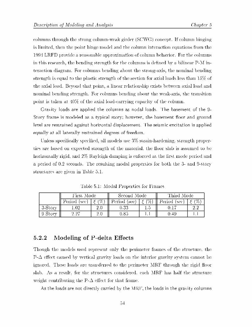
Description of Modeling and Analysis Chapter 5
columns through the strong column-weak girder (SCWG) concept. If column hinging
is limited, then the point hinge model and the column interaction equations from the
1994 LRFD provide a reasonable approximation of column behavior. For the columns
in this research, the bending strength for the columns is de�ned by a bilinear P-M in-
teraction diagram. For columns bending about the strong-axis, the nominal bending
strength is equal to the plastic strength of the section for axial loads less than 15% of
the axial load. Beyond that point, a linear relationship exists between axial load and
nominal bending strength. For columns bending about the weak-axis, the transition
point is taken at 40% of the axial load-carrying capacity of the column.
Gravity loads are applied the columns as nodal loads. The basement of the 9-
Story frame is modeled as a typical story; however, the basement oor and ground
level are restrained against horizontal displacement. The seismic excitation is applied
equally at all laterally restrained degrees of freedom.
Unless speci�cally speci�ed, all models use 3% strain-hardening, strength proper-
ties are based on expected strength of the material, the oor slab is assumed to be
horizontally rigid, and 2% Rayleigh damping is enforced at the �rst mode period and
a period of 0.2 seconds. The resulting modal properties for both the 3- and 9-story
structures are given in Table 5.1.
Table 5.1: Modal Properties for Frames
First Mode Second Mode Third ModePeriod (sec) � (%) Period (sec) � (%) Period (sec) � (%)
3-Story 1.02 2.0 0.33 1.5 0.17 2.29-Story 2.27 2.0 0.85 1.1 0.49 1.1
5.2.2 Modeling of P-delta E�ects
Though the models used represent only the perimeter frames of the structure, the
P-� e�ect caused by vertical gravity loads on the interior gravity system cannot be
ignored. These loads are transferred to the perimeter MRF through the rigid oor
slab. As a result, for the structures considered, each MRF has half the structure
weight contributing the P-� e�ect for that frame.
As the loads are not directly carried by the MRF, the loads in the gravity columns
54
Chapter 5 Description of Modeling and Analysis
cannot simply be lumped with the loads applied directly to the columns of the lateral
system as that assumption generally results in an over-estimation of column demands.
Therefore, the e�ect is considered by attaching an elastic P-� column to the two-
dimensional model with frame elements. The P-� column is given a very high axial
sti�ness and negligible bending sti�ness, so that the column can take the de ected
shape of the MRF without contributing to the moment-resisting system. The analysis
program uses a geometric sti�ness matrix based on the axial load in the columns under
gravity loads only, as described in Section 5.3.4.
5.3 Evaluation Platform and Implementation
In order to evaluate the behavior of the structural model, an analysis tool capable
of analyzing inelastic structural behavior during seismic loads is required. This tool
also needs to include the basic behavior of the di�erent control elements. A �nite
element nonlinear dynamic analysis code was written utilizing MATLAB1 to evaluate
the systems for this study.
Currently, the code is limited to planar, two-dimensional, structures. Each node
can have up to three degrees-of-freedom, translations in the x- and y-direction and
rotation about the out-of-plane axis. The code has provisions for specifying nodal
displacement constraints, allowing for the slaving of one degree-of-freedom to another.
The mass is assumed to be lumped at the nodes, so that the structural mass matrix is
diagonal. Also, loads may only be applied at the nodes of the model. Viscous damping
inherent in the structure is assumed to be of the Rayleigh type. The damping matrix
is assumed to be constant, so the sti�ness proportional damping is based only on the
initial sti�ness of the system. However, di�erent amounts of damping can be speci�ed
to di�erent element types.
Most engineering analyses adopt a nonlinear beam model in which the plasti�ed
region is represented as a point while the remainder of the structural member remains
elastic (Chen and Powell 1982; Allahabadi 1987). Lumped models typically consist
1MATLAB is a registered trademark of The MathWorks Inc., 24 Prime Park Way, Natic, MA01760-1415
55
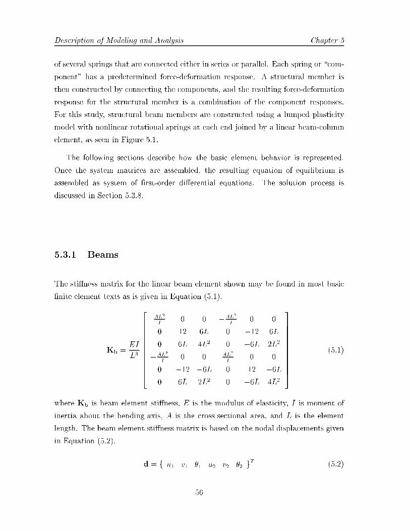
Description of Modeling and Analysis Chapter 5
of several springs that are connected either in series or parallel. Each spring or \com-
ponent" has a predetermined force-deformation response. A structural member is
then constructed by connecting the components, and the resulting force-deformation
response for the structural member is a combination of the component responses.
For this study, structural beam members are constructed using a lumped plasticity
model with nonlinear rotational springs at each end joined by a linear beam-column
element, as seen in Figure 5.1.
The following sections describe how the basic element behavior is represented.
Once the system matrices are assembled, the resulting equation of equilibrium is
assembled as system of �rst-order di�erential equations. The solution process is
discussed in Section 5.3.8.
5.3.1 Beams
The sti�ness matrix for the linear beam element shown may be found in most basic
�nite element texts as is given in Equation (5.1).
Kb =EI
L3
266666666664
AL2
I0 0 �AL2
I0 0
0 12 6L 0 �12 6L
0 6L 4L2 0 �6L 2L2
�AL2
I0 0 AL2
I0 0
0 �12 �6L 0 12 �6L0 6L 2L2 0 �6L 4L2
377777777775
(5.1)
where Kb is beam element sti�ness, E is the modulus of elasticity, I is moment of
inertia about the bending-axis, A is the cross-sectional area, and L is the element
length. The beam element sti�ness matrix is based on the nodal displacements given
in Equation (5.2).
d = f u1 v1 �1 u2 v2 �2 gT (5.2)
56

Chapter 5 Description of Modeling and Analysis
5.3.2 Hysteresis Modeling
Various hysteretic models for the restoring force of an inelastic structure have been
developed in recent years (Baber and Noori 1985; Baber and Noori 1986). The
model chosen for the nonlinear rotational spring is the Bouc-Wen (1976) smooth-
varying hysteretic model. This model includes a number of parameters, allowing
a mathematically tractable state-space representation capable of expressing several
hysteretic properties.
The restoring force, (fR)i, for a single nonlinear element i may be decomposed
into two parts, (fE)i and (fH)i, representing the elastic and hysteretic components
respectively. The restoring force can then be written with the subscript i implied as:
fR = fE + fH = ke r(t) + kh z(t) = � kT (xa � xb) + (1� �) kT z(t) (5.3)
where � is ratio of the post-yielding to pre-yielding sti�ness and kT is the pre-yielding
sti�ness. The variable r(t) is the relative deformation, xa and xb are the absolute
displacements at nodes a and b respectively, and z(t) is the corresponding variable
introduced to describe the hysteretic component. The elastic component is used
to represent the strain-hardening in the element. The force-deformation curve is
described by:
_z = _rdz
dr= _r[A� (� + sgn( _rz))jzjn] (5.4)
where A, �, , n are shaping parameters (Wen 1976) and the term in square brackets,
dz=dr, describes the hysteretic curve. Since we require dz=dr to be unity at small
values of z, then A = 1 . The yield displacement Y = (� + )1=n; taking � and as
equal, Equation (5.4) can now be written as:
_z = _rh1� 0:5(1 + sgn( _rz))
��� zY
���ni (5.5)
The resulting hysteretic behavior described above is a stable force-deformation
curve. The use of constant strain-hardening with the stable hysteretic loop ignores
the presence of cyclic hardening and does not permit modeling of deterioration due to
local instabilities. These e�ects could be captured through modi�cation of the above
57

Description of Modeling and Analysis Chapter 5
equations.
Now consider a structure idealized by an n degree-of-freedom system under a one-
dimensional earthquake ground motion. The equation of motion for the system can
be expressed as:
M �x(t) +C _x(t) +KE x(t) +KH z(t) = �M flg �ug(t) = Fg(t) (5.6)
in which x(t) is an vector containing the displacement of each degree of freedom
relative to the ground, and z(t) is a vector containing the corresponding hysteretic
information for each element. M is the mass matrix and C is the viscous damping
matrix. The ground motion, Fg, is found by mapping the horizontal ground accelera-
tion, �ug, to the horizontal degrees of freedom through the vector flg and multiplying
by M. As in the single element case, the elastic and hysteretic components of the
structural restoring force can be separated such that:
FR = FE + FH = KE x(t) +KH z(t) (5.7)
so that the restoring force is a function of both x(t) and z(t). The equation of motion
for the system can be written in a nonlinear state-space format, as follows:8>><>>:
_x(t)
�x(t)
z(t)
9>>=>>; =
2664
0 I 0
�M�1KE �M�1C �M�1KH
0 [dz=dx] 0
37758>><>>:
x(t)
_x(t)
z(t)
9>>=>>;+
2664
0
M�1
0
3775Fg(t)
(5.8)
where [dz=dx] is a non-square matrix function found by:
[dz=dx] = [dz=dr]Brx (5.9)
and [dz=dr] is a diagonal matrix function of _x(t) and z(t) with entries dzi=dri found
in Equation (5.5), and Brx is a non-square matrix mapping the displacements x(t) to
the relative deformations r(t). The system can now be solved using any of a number
58
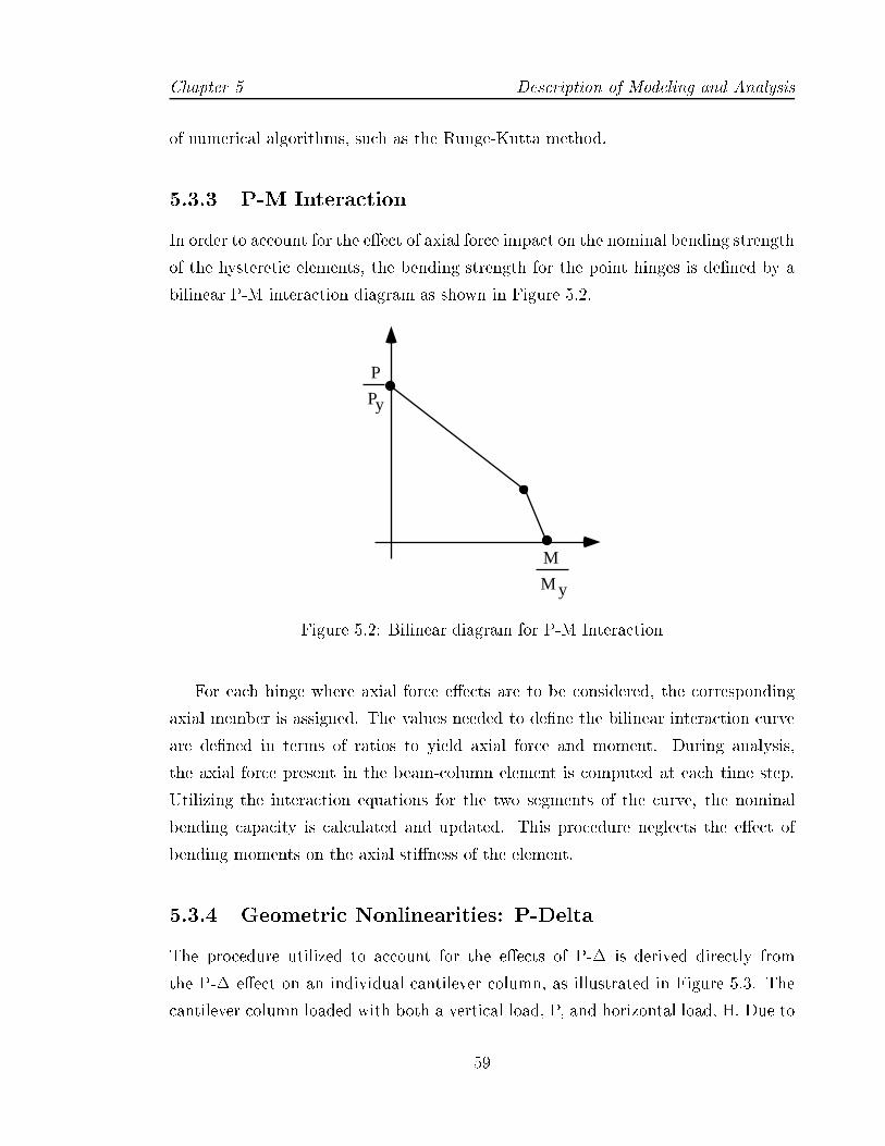
Chapter 5 Description of Modeling and Analysis
of numerical algorithms, such as the Runge-Kutta method.
5.3.3 P-M Interaction
In order to account for the e�ect of axial force impact on the nominal bending strength
of the hysteretic elements, the bending strength for the point hinges is de�ned by a
bilinear P-M interaction diagram as shown in Figure 5.2.
P
Py
M
M y
Figure 5.2: Bilinear diagram for P-M Interaction
For each hinge where axial force e�ects are to be considered, the corresponding
axial member is assigned. The values needed to de�ne the bilinear interaction curve
are de�ned in terms of ratios to yield axial force and moment. During analysis,
the axial force present in the beam-column element is computed at each time step.
Utilizing the interaction equations for the two segments of the curve, the nominal
bending capacity is calculated and updated. This procedure neglects the e�ect of
bending moments on the axial sti�ness of the element.
5.3.4 Geometric Nonlinearities: P-Delta
The procedure utilized to account for the e�ects of P-� is derived directly from
the P-� e�ect on an individual cantilever column, as illustrated in Figure 5.3. The
cantilever column loaded with both a vertical load, P, and horizontal load, H. Due to
59

Description of Modeling and Analysis Chapter 5
a horizontal displacement at the top of the column, �, the vertical load now generates
an additional bending moment at the bottom of the column.
P
H
Le
P
H
∆e
H + (P/Le) ∆e
Le
Figure 5.3: P-� Forces Associated with a Gravity Column
Alternatively, the problem can be reformulated so that the horizontal load in the
column is augmented to result in the same bending moment at the base of the column.
This additional horizontal load, or geometric shear, is given by P (�e=Le), where Le is
the height of the column. The equilibrium equation for the column in the horizontal
direction is now:
k�e = H+ P�e
Le
(5.10)
where k is the lateral sti�ness of the column. By rearranging the terms in Equa-
tion (5.10), the following expression results:
�k � P
L
�� = keff� = H (5.11)
were keff is the e�ective lateral sti�ness for the column. Thus, the introduction of
the P-� is equivalent to reducing the lateral sti�ness of the column. Though the
resulting variation of bending moment over the length of the column is not exactly
the same as in the original case, this method provides a reasonable approximation.
The above relationship between forces and the lateral translations at the top and
bottom of a column can be written in matrix form (White and Hajjar 1991) as:
(fxi
fxj
)=
P
Le
"1 �1�1 1
#(uxi
uxj
)(5.12)
60

Chapter 5 Description of Modeling and Analysis
where P is the axial force in the column (negative for compression), and Le is the col-
umn height. This matrix also corresponds to the geometric sti�ness of a truss element.
The full P-� contribution from a gravity column at any level can be represented in
a global matrix solution simply by assembling the sti�ness matrix of Equation (5.12)
into the global structure elastic sti�ness matrix,KE. If a rigid oor constraint is used,
these element sti�ness matrices can be grouped together onto one structure node per
oor.
The analysis program uses a geometric sti�ness matrix based on the axial load
in the columns under gravity loads only. As a result, since the geometric sti�ness
matrices are only calculated once, this method provides a �rst-order approximation
of a second-order elastic analysis.
5.3.5 Viscous Damper
The viscous dampers studied are assumed to be linear, and their constitutional force-
deformation relationship can be expressed as follows:
Fd(t) = Cd _ud(t) (5.13)
where Fd(t) and _ud(t) are the resistance force and deformation of the dampers re-
spectively. Cd is the damping constant of the VS damper. In the frequency domain,
assuming ud(t) = ud;max sin(!t), the above equation becomes:
Fd(t) = Cd ! ud;max cos(!t) = K00
d ud;max cos(!t) (5.14)
where K00
d is the loss sti�ness for the VS damper (Kasai, Munshi, Lai, and Maison
1993).
As mentioned in Section 4.4.2, the damper-brace component is collectively referred
to as the damper system. The mathematical model of the damper system is shown
in Figure 5.3.5, where KB is the sti�ness of the brace used to install the damper in
the frame structure. The brace element, if not assumed to be rigid, is modeled as a
linear truss element.
61

Description of Modeling and Analysis Chapter 5
KB
KD
CD
Figure 5.4: Schematic Diagram for Viscoelastic Damper
The equations for the damper element, in matrix format, can be written as
(Fd;i
Fd;j
)= Cd
"1 �1�1 1
#(_ud;i
_ud;j
)+Kd
"1 �1�1 1
#(ud;i
ud;j
)(5.15)
where ud;i and ud;j are the displacements at the ith and jth end of the damper re-
spectively. The above equations are similar to those for linear truss elements, except
that it contains both velocity and displacement terms in the local coordinate system.
After transformation to the global coordinate system, the matrix corresponding to
the displacement proportional terms are assembled into the global elastic sti�ness
matrix, KE, while the matrix corresponding to the velocity proportional terms are
assembled into the global damping matrix, C.
5.3.6 Friction Pendulum Isolation (FPS) Element
The principles of operation of the FPS bearing are discussed in Section 3.2.2. The
bearing consists of a spherical sliding surface and an articulated slider that is lined
with a high capacity bearing material. The basic model implemented for the bearing
is similar to that of the nonlinear spring. The frictional force that is mobilized at
the sliding interface of sliding bearings depends on the normal load, bearing pressure,
direction and value of sliding velocity and composition of the sliding interface.
At an instance of time, the bearing carries a weight and is subjected to vertical
acceleration and additional seismic load due to overturning moments e�ects. The
force-displacement relationship that develops at the sliding interface are described
by:
Ff =W �
Ruf + �SW
�zf = ke;fuf + kh;f (5.16)
62
Chapter 5 Description of Modeling and Analysis
where:
W � = W (1 +�ufg+PSW
) (5.17)
is the normal load on the sliding interface, PS is the normal load on the bearing, W is
the seismic weight of the structure carried by the bearing, and �uf is the acceleration
across the bearing surface. The direct e�ects of variations in the normal force on the
behavior of the FPS bearing are to instantaneously change the sti�ness and friction
force of the bearing. However, approximating the normal load such that W � = W re-
sults in nearly the same global isolation system response and superstructure response.
This e�ect has been demonstrated by comparison of analytical results to shake table
results of a seven-story model in which the axial forces on individual bearings varied
from 0 to twice the gravity load (Al-Hussaini, Zayas, and Constantinou 1994).
Also, zf is a dimensionless variable which are governed by a system of di�erential
equations based on the Bouc-Wen model described above, such that
_zf = D�1y ( _uf � �ij _uf jjzf jn�1zf � _uf jzf jn) (5.18)
where Dy is the yield displacement; and � and govern the shape of the hysteresis
loop described in Section 5.3.2. When yielding commences, provided that
1
� + = 1 (5.19)
then zf is bounded by values �1 and account for the direction of sliding forces.
The coeÆcient of sliding friction, is described by
�S = fmax � (fmax � fmin) exp�aj _uj (5.20)
where �S is the sliding coeÆcient of friction, _uf is the velocity of sliding, fmax is
the coeÆcient of sliding friction at high velocity, and fmin is the coeÆcient of sliding
friction at low velocity, and a is a coeÆcient controlling the dependency of friction
on sliding velocity. In general, the parameters fmax, fmin, and a are determined ex-
perimentally depending on bearing pressure, surface roughness, and the composition
of PTFE.
63

Description of Modeling and Analysis Chapter 5
As with the nonlinear spring element, the elastic and hysteretic components of
the structural restoring force can be separated such that:
Ff = FE;f + FH;f = KEf x(t) +KHf z(t) (5.21)
where KEf and KHf are the matrix formulation of the expressions given in Equa-
tion (5.16). The element also places the entry dzi=dri, as de�ned in Equation (5.18),
into [dz=dr], given in Equation (5.8).
5.3.7 Active Control
Speci�c elements are available to represent the actuators and sensors in the active
control system. Both require information regarding the noise bandwith, and a satu-
ration level for the actuator element. The controller algorithms integrated with the
above analytical model are linear dynamic output feedback controllers of the form:
_xc(t) = Acxc(t) +Bcy(t) (5.22)
w(t) = Ccxc(t) +Dcy(t) (5.23)
where xc(t) is the state vector of the dynamic controller, y(t) is the sensor reading
vector, w(t) is the controller command signal, and the constant matrices Ac, Bc, Cc
and Dc are the linear state description of the regulator.
The controller command signal w(t) is mapped to forces applied to the structure
by the equation:
Fu(t) = Buw(t) (5.24)
which is an additional force input to the state equations with the same mapping as
Fg in Equation (5.8). The sensor measurements are described by mapping the states
to the absolute accelerations at the sensor locations
y(t) = Cy(�M�1C_x(t) +�M�1KEx(t) +�M�1KHz(t) + Fu(t)) (5.25)
where Cy selects which accelerations are available. Equation (5.25) is combined with
64
Chapter 5 Description of Modeling and Analysis
the uncontrolled structure state space equation in Equation (5.8) to form the con-
trolled system with the augmented state vector xs(t) = fx _x z xcgT with the addi-
tional states of the controller added to the original state vector. The controller loop
from the sensors to the actuator forces is algebraically closed to form a state space
equation:
_xs(t) = A(xs(t)) xs(t) +BwFg (5.26)
which is used to perform the nonlinear time history analysis.
5.3.8 Solution Procedure
Based on the above discussions, the analysis platform is implemented in MATLAB
. Utilizing MATLAB as the platform for implementation o�ers the advantages of
simplicity of coding, a wide variety of inbuilt functions for matrix analysis, toolboxes
for active control linear analysis and design, and graphical functions for visualization
of the results. However, analyses performed using MATLAB are fairly ineÆcient
as the resulting code is not pre-compiled. Given the problem size, eÆciency and
memory management were special concerns. Care was taken to vectorize operations
as much as possible, as these operations are faster within MATLAB. In-built utilities
for sparse matrix operations and storage were used, and temporary variables cleared
from memory as soon as possible.
An input �le needs to be generated that de�nes the model, both its structural
and control elements. Sections that must be included in the input are: node def-
inition, boundary conditions, nodal constraints, point masses, material properties,
element de�nitions, static nodal loads, control elements, and the acceleration record
for seismic load. From this information the �nite element model is generated. The sys-
tem matrices are assembled, and the state-space model described in Equations (5.8)
and (5.26) is generated. The di�erent analyses available include a modal analysis
based on initial system properties, static linear analysis, and nonlinear time-history
analysis.
The time history analysis is performed using one of the built-in solver for or-
dinary di�erential equations. To use the MATLAB ordinary di�erential equation
65

Description of Modeling and Analysis Chapter 5
{ x, z }, F
AnyElements with PM-Interaction Surfaces
Defined?
Calculate current axialforceUpdate moment capacity
PM_Interaction
AnyFPS Bearing Elements? Determine relative
velocityUpdate µs
Friction Coefficient
yes
no
Update [dz/dx]
Solve for {xd, zd}
{xd, zd}
Figure 5.5: Flowchart of StructODE function
(ODE) solvers, you must rewrite such equations as an equivalent system of �rst-order
di�erential equations as in Equation (5.26). Once the equation is represented in this
way, it can be coded as a function that a MATLAB ODE-solver can use. After test-
ing the di�erent solvers available, the sti�-system solver ode15s was chosen. The
ode15s is a variable-order, multistep solver based on the numerical di�erentiation
formulas. Optionally it uses the backward di�erentiation formulas (also known as
Gear's method) that are usually less eÆcient (Shampine and Reichelt 1998). The
analytical expression for the Jacobian matrix is provided for increased eÆciency. At
initial time-step, perform a linear static analysis under speci�ed static nodal loads.
The results are used to initialize the structure states for the dynamic analysis. At
every function evaluation, the process illustrated in Figure 5.5 are taken.
The output of the time-history analysis is a matrix containing the structure states
66
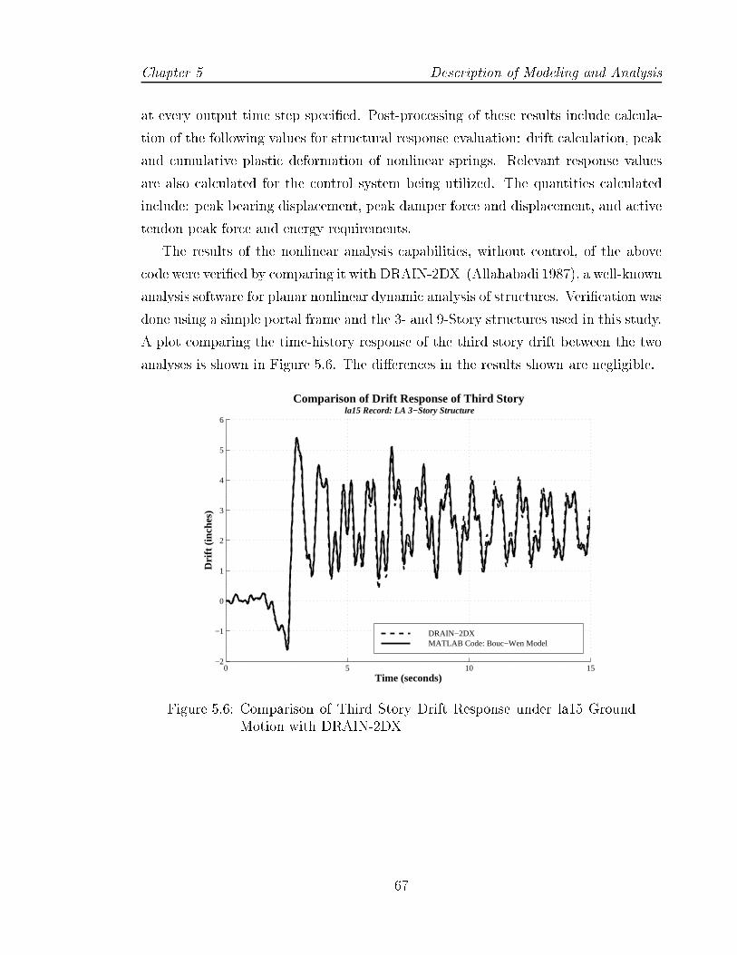
Chapter 5 Description of Modeling and Analysis
at every output time step speci�ed. Post-processing of these results include calcula-
tion of the following values for structural response evaluation: drift calculation, peak
and cumulative plastic deformation of nonlinear springs. Relevant response values
are also calculated for the control system being utilized. The quantities calculated
include: peak bearing displacement, peak damper force and displacement, and active
tendon peak force and energy requirements.
The results of the nonlinear analysis capabilities, without control, of the above
code were veri�ed by comparing it with DRAIN-2DX (Allahabadi 1987), a well-known
analysis software for planar nonlinear dynamic analysis of structures. Veri�cation was
done using a simple portal frame and the 3- and 9-Story structures used in this study.
A plot comparing the time-history response of the third story drift between the two
analyses is shown in Figure 5.6. The di�erences in the results shown are negligible.
0 5 10 15−2
−1
0
1
2
3
4
5
6
Time (seconds)
Drif
t (in
ches
)
Comparison of Drift Response of Third Story la15 Record: LA 3−Story Structure
DRAIN−2DX MATLAB Code: Bouc−Wen Model
Figure 5.6: Comparison of Third Story Drift Response under la15 GroundMotion with DRAIN-2DX
67

Chapter 6
Evaluation of Seismic Demands
6.1 Introduction
This chapter focuses on the quanti�cation of seismic demands at the structure level
for the 3- and 9-Story steel moment-resisting frames (SMRF) in Los Angeles. The
description for the structure design and basic control parameters is given in Chapter 4.
The behavior and response of the structures with and without control systems is
studied by subjecting nonlinear analytical models of the structures to sets of ground
motions representative of di�erent hazard levels.
The structural demand parameters used to evaluate and quantify the response
of the structures include roof and interstory drift angle, hysteretic energy demands
and peak oor accelerations. For each control system analyzed, the e�ect of varying
control parameters on the seismic demand of the structures is determined. From
these investigations, the performance of one design per control system is evaluated
based on characteristic values given in FEMA 273 (BSSC 1997), listed in Table 2.1.
A comparison between the di�erent systems is then presented.
As a representative values of the response, the primary statistic of interest is
a \best estimate" or central-estimate of the data referred to as the median1 value.
Also of interest are the maximum, 84th percentile, which is determined assuming
a logarithmic distribution to the data, and the standard deviation of the natural
log of the data, �ln, which is used as an indicator of the dispersion in the data.
1The median is more precisely de�ned as the geometric mean of the data that is found as theexponential of the average of the natural log of the observed values
68
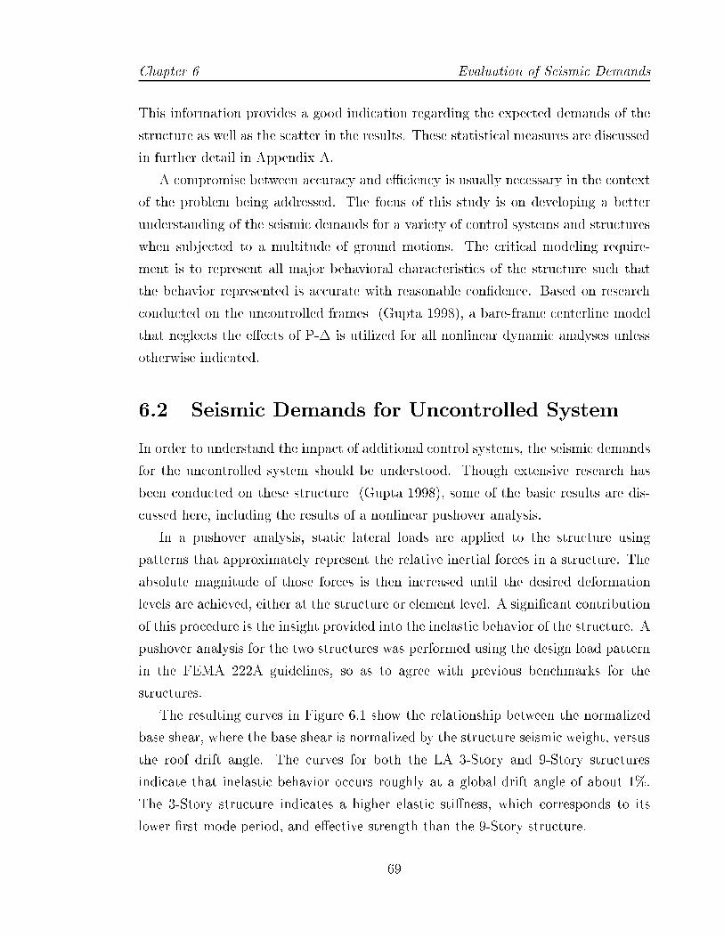
Chapter 6 Evaluation of Seismic Demands
This information provides a good indication regarding the expected demands of the
structure as well as the scatter in the results. These statistical measures are discussed
in further detail in Appendix A.
A compromise between accuracy and eÆciency is usually necessary in the context
of the problem being addressed. The focus of this study is on developing a better
understanding of the seismic demands for a variety of control systems and structures
when subjected to a multitude of ground motions. The critical modeling require-
ment is to represent all major behavioral characteristics of the structure such that
the behavior represented is accurate with reasonable con�dence. Based on research
conducted on the uncontrolled frames (Gupta 1998), a bare-frame centerline model
that neglects the e�ects of P-� is utilized for all nonlinear dynamic analyses unless
otherwise indicated.
6.2 Seismic Demands for Uncontrolled System
In order to understand the impact of additional control systems, the seismic demands
for the uncontrolled system should be understood. Though extensive research has
been conducted on these structure (Gupta 1998), some of the basic results are dis-
cussed here, including the results of a nonlinear pushover analysis.
In a pushover analysis, static lateral loads are applied to the structure using
patterns that approximately represent the relative inertial forces in a structure. The
absolute magnitude of those forces is then increased until the desired deformation
levels are achieved, either at the structure or element level. A signi�cant contribution
of this procedure is the insight provided into the inelastic behavior of the structure. A
pushover analysis for the two structures was performed using the design load pattern
in the FEMA 222A guidelines, so as to agree with previous benchmarks for the
structures.
The resulting curves in Figure 6.1 show the relationship between the normalized
base shear, where the base shear is normalized by the structure seismic weight, versus
the roof drift angle. The curves for both the LA 3-Story and 9-Story structures
indicate that inelastic behavior occurs roughly at a global drift angle of about 1%.
The 3-Story structure indicates a higher elastic sti�ness, which corresponds to its
lower �rst mode period, and e�ective strength than the 9-Story structure.
69

Evaluation of Seismic Demands Chapter 6
0 0.005 0.01 0.015 0.02 0.025 0.03 0.035 0.04 0.045 0.050
0.05
0.1
0.15
0.2
0.25
0.3
0.35
Roof Drift Angle
Nor
mal
ized
Bas
e S
hear
Roof Drift Angle vs. Normalized Base Shear Nonlinear Pushover Analysis: LA 3− and 9−Story
LA 3−StoryLA 9−Story
Figure 6.1: Global Pushover Curves for LA 3- and 9-Story Structures
A nonlinear dynamic analysis is necessary to more accurately capture the response
of the structure under seismic loads. The statistical values for the roof drift angle
demands for both structures are given in Table 6.1. Based on the results of the
pushover analyses, the median values of the roof drift angle indicate minor inelastic
behavior under the 50 in 50 set of ground motions. The roof drift angles under the 2
in 50 set of excitations are still below the collapse prevention limit of 5%. Signi�cant
dispersion is present in the data, however, as indicated by the high values of �ln.
While the dispersion remains fairly constant between the 50 in 50 set and 10 in 50
set, it is signi�cantly larger for the results of the simulations under the 2 in 50 set.
The dispersion is also higher in the results of the 3-Story frame as compared to those
for the 9-Story frame.
The drift demands over the height of the structures can be obtained from Fig-
ures 6.2 and 6.3. The values for story drift angle are indicated as points between
the bounding oors that are connected by straight lines. This plotting convention
is adopted throughout this report. Median values of story drift angle correlate well
with basic expected structural response (BSSC 1997): little inelasticity under fre-
quent events and collapse prevention under severe excitations. In the 50 in 50 set
70

Chapter 6 Evaluation of Seismic Demands
Table 6.1: Statistics on Roof Drift Angle Demands
Structure Ground Motion Median 84th Perc. Maximum �ln
3-Story50 in 50 0.0112 0.0169 0.0300 0.4110 in 50 0.0159 0.0241 0.0371 0.412 in 50 0.0283 0.0519 0.0770 0.61
9-Story50 in 50 0.0067 0.0094 0.0110 0.3510 in 50 0.0114 0.0162 0.0197 0.352 in 50 0.0160 0.0261 0.0306 0.49
of ground motions, an average of 1% drift is observed for both the 3- and 9-Story
structures. Also, the distribution of drift demands over the height of the structures is
fairly constant in both cases. As the excitations become more severe, drift demands
are not evenly distributed.
0 0.005 0.01 0.015 0.02 0.025 0.03 0.035 0.04 0.045 0.050
1
2
3
Median Values for Peak Story Drift Angles for 3 Earthquake Sets LA 3−Story Structure: α = 3%, no P−∆
Drift Angle
Flo
or L
evel
2 in 5010 in 50 50 in 50
Figure 6.2: Median Values for Peak Story Drift Angle for 3-Story Structure,All Sets of Ground Motions
For the 3-Story structure, the peak drift angle occurs in the third story for all
three sets of ground motions. The 10 in 50 set induce a peak drift angle of about
2.4%, which increases to about 4.7% under the 2 in 50 set. For the 9-Story structure,
the location of peak drift occurs in the eighth story for the 10 in 50 set; however, in
71

Evaluation of Seismic Demands Chapter 6
0 0.005 0.01 0.015 0.02 0.025 0.03 0.035 0.04 0.045 0.05
1
2
3
4
5
6
7
8
9
Median Values for Peak Story Drift Angles for 3 Earthquake Sets LA 9−Story Structure: α = 3%, no P−∆
Drift Angle
Flo
or L
evel
2 in 5010 in 50 50 in 50
Figure 6.3: Median Values for Peak Story Drift Angle for 9-Story Structure,All Sets of Ground Motions
the 2 in 50 set, the location of peak drifts has moved to the third story. As with the
roof drift angle, dispersion values in the data are quite high especially under the 2
in 50 set of excitations, as seen in Figures 6.4 and 6.5. In the 3-Story structure, the
increase in dispersion evenly increases in each story with increasing excitations. For
the 9-Story structure the dispersion is fairly similar under the 50 in 50 set and 10 in
50 set of excitations. The distribution under the 2 in 50 set, however, is signi�cantly
di�erent, with the highest values present around the second and third stories. The
standard deviation of the natural logarithm of the data, �ln(Æ), is used as an indicator
of the dispersion of the results. The dispersion of the peak drift values for each story
of the 3- and 9-story structures are shown in Figures 6.4 and 6.5. For both structures
the scatter in the data is signi�cant. The story dispersion for the 3-story structure
consistently increases with increasing hazard for all three stories. A di�erent behavior
is present in the 9-story structure, where the lines for di�erent hazard levels cross one
another. While the lower stories indicate a signi�cant increase in dispersion in the 2
in 50 Set, the dispersion in the upper three stories decreases below that of the 50 in
50 Set.
72
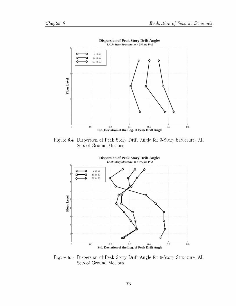
Chapter 6 Evaluation of Seismic Demands
0 0.1 0.2 0.3 0.4 0.5 0.6
1
2
3
Dispersion of Peak Story Drift Angles LA 3−Story Structure: α = 3%, no P−∆
Std. Deviation of the Log. of Peak Drift Angle
Flo
or L
evel
2 in 50
10 in 50
50 in 50
Figure 6.4: Dispersion of Peak Story Drift Angle for 3-Story Structure, AllSets of Ground Motions
0 0.1 0.2 0.3 0.4 0.5 0.6
1
2
3
4
5
6
7
8
9
Dispersion of Peak Story Drift Angles LA 9−Story Structure: α = 3%, no P−∆
Flo
or L
evel
Std. Deviation of the Log. of Peak Drift Angle
2 in 50
10 in 50
50 in 50
Figure 6.5: Dispersion of Peak Story Drift Angle for 9-Story Structure, AllSets of Ground Motions
73
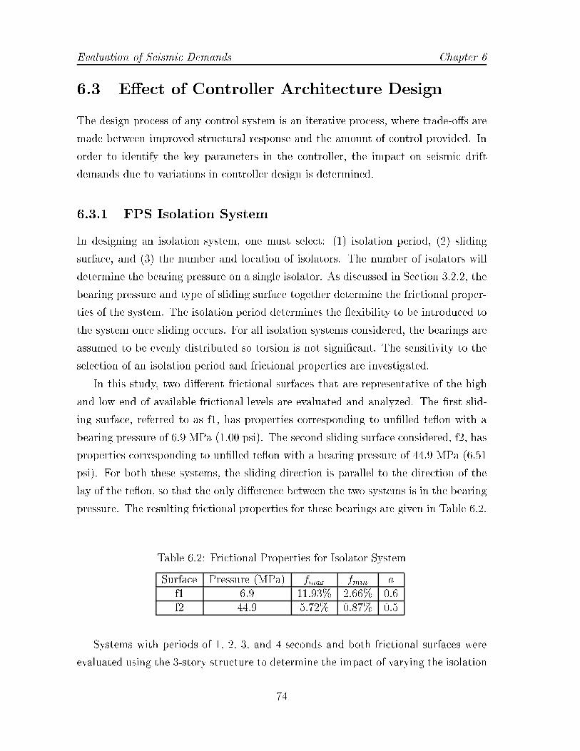
Evaluation of Seismic Demands Chapter 6
6.3 E�ect of Controller Architecture Design
The design process of any control system is an iterative process, where trade-o�s are
made between improved structural response and the amount of control provided. In
order to identify the key parameters in the controller, the impact on seismic drift
demands due to variations in controller design is determined.
6.3.1 FPS Isolation System
In designing an isolation system, one must select: (1) isolation period, (2) sliding
surface, and (3) the number and location of isolators. The number of isolators will
determine the bearing pressure on a single isolator. As discussed in Section 3.2.2, the
bearing pressure and type of sliding surface together determine the frictional proper-
ties of the system. The isolation period determines the exibility to be introduced to
the system once sliding occurs. For all isolation systems considered, the bearings are
assumed to be evenly distributed so torsion is not signi�cant. The sensitivity to the
selection of an isolation period and frictional properties are investigated.
In this study, two di�erent frictional surfaces that are representative of the high
and low end of available frictional levels are evaluated and analyzed. The �rst slid-
ing surface, referred to as f1, has properties corresponding to un�lled te on with a
bearing pressure of 6.9 MPa (1.00 psi). The second sliding surface considered, f2, has
properties corresponding to un�lled te on with a bearing pressure of 44.9 MPa (6.51
psi). For both these systems, the sliding direction is parallel to the direction of the
lay of the te on, so that the only di�erence between the two systems is in the bearing
pressure. The resulting frictional properties for these bearings are given in Table 6.2.
Table 6.2: Frictional Properties for Isolator System
Surface Pressure (MPa) fmax fmin af1 6.9 11.93% 2.66% 0.6f2 44.9 5.72% 0.87% 0.5
Systems with periods of 1, 2, 3, and 4 seconds and both frictional surfaces were
evaluated using the 3-story structure to determine the impact of varying the isolation
74
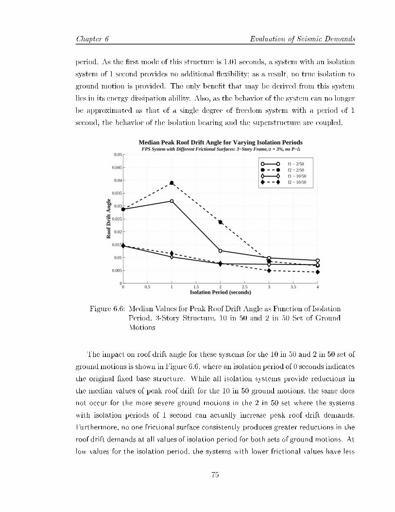
Chapter 6 Evaluation of Seismic Demands
period. As the �rst mode of this structure is 1.01 seconds, a system with an isolation
system of 1 second provides no additional exibility; as a result, no true isolation to
ground motion is provided. The only bene�t that may be derived from this system
lies in its energy dissipation ability. Also, as the behavior of the system can no longer
be approximated as that of a single degree of freedom system with a period of 1
second, the behavior of the isolation bearing and the superstructure are coupled.
0 0.5 1 1.5 2 2.5 3 3.5 40
0.005
0.01
0.015
0.02
0.025
0.03
0.035
0.04
0.045
0.05
Isolation Period (seconds)
Roo
f Drif
t Ang
le
Median Peak Roof Drift Angle for Varying Isolation Periods FPS System with Different Frictional Surfaces: 3−Story Frame, α = 3%, no P−∆
f1 − 2/50 f2 − 2/50 f1 − 10/50f2 − 10/50
Figure 6.6: Median Values for Peak Roof Drift Angle as Function of IsolationPeriod, 3-Story Structure, 10 in 50 and 2 in 50 Set of GroundMotions
The impact on roof drift angle for these systems for the 10 in 50 and 2 in 50 set of
ground motions is shown in Figure 6.6, where an isolation period of 0 seconds indicates
the original �xed base structure. While all isolation systems provide reductions in
the median values of peak roof drift for the 10 in 50 ground motions, the same does
not occur for the more severe ground motions in the 2 in 50 set where the systems
with isolation periods of 1 second can actually increase peak roof drift demands.
Furthermore, no one frictional surface consistently produces greater reductions in the
roof drift demands at all values of isolation period for both sets of ground motions. At
low values for the isolation period, the systems with lower frictional values have less
75

Evaluation of Seismic Demands Chapter 6
of an impact on roof drift demands, while the reverse is true at higher isolation levels.
As sliding surface f2 has a smaller coeÆcient of friction than f1, systems with those
surfaces reach their sliding force more quickly. This behavior is desirable at high
values of isolation period, where the system period is shifted to values of reduced
spectral accelerations.
Because provisions must be made to allow for the lateral motion of the structure at
the base, generally through a gap with the surrounding area, a key issue in isolation
system design is maintaining bearing displacements as low as possible while still
achieving the desired structural response. Systems with the sliding surface f2 isolator
generally result in signi�cantly higher bearing displacements then those associated
with the corresponding f1 system (see Table 6.3). As the systems are identical except
for the pressure on the bearings, correct estimation of the building weight is critical in
determining the system's performance. For the systems with isolation periods of 1 and
2 seconds, bearing displacements are greater than 20% of their radius of curvature. As
a result, the small angle approximations utilized in describing the bearing behavior
no longer hold, and signi�cant vertical motion occurs in the bearing, which is not
captured in the model analyzed. This vertical motion leads to a signi�cant increase
in axial forces in the columns (Llera and Almazan 1998). This e�ect reduces the
columns load carrying capacity and may result in higher drift demands than indicated
by these results. For the same isolation period, f2 systems result in higher median
bearing displacements, as their sliding force is lower.
Table 6.3: Peak Bearing Response for 3-Story Structure Isolation Bearing: 2in 50 Set of Ground Motions
IsolationPeriod
Median (inches) % Curvaturef1 f2 f1 f2
1 sec 4.78 5.45 49 562 sec 12.4 17.2 31 433 sec 15.7 24.7 18 284 sec 15.2 21.3 10 14
The scatter in the response is also greater for bearings with surface f2 than their
counterparts with sliding surface f1, as shown in Figure 6.7. The scatter also in-
creases with increasing isolation period. In a few cases, the bearing displacement
76

Chapter 6 Evaluation of Seismic Demands
exceeds three feet, which would may not be feasible for implementation depending
on the structure's actual surroundings. At the high isolation periods typically used
for isolation systems, the improvement gained by using sliding surfaces with lower
frictional levels is minor compared to the increase in bearing displacement; therefore
systems with higher values of friction are more desirable desirable.
T1, f1 T1, f2 T2, f1 T2, f2 T3, f1 T3, f2 T4, f1 T4, f20
10
20
30
40
50
60
Drif
t Ang
le
Maximum Bearing Displacement for FPS System 2 in 50 Set of Earthquakes: 3−Story Structure, α = 3%, no P−∆
Figure 6.7: Peak Bearing Displacements for 3-Story Frame with FPS Isola-tion, 2 in 50 Set of Ground Motions
The distribution of story drift over the height of the structure is fairly constant
under the 10 in 50 ground motions as the superstructure remains essentially linear,
as seen in Figure 6.8. However, the story drift demands under the 2 in 50 Set for
the system with an isolation period of 2 seconds are beyond the desirable range, as
shown in Figure 6.9. Little additional reduction in drift demands is gained by using
an isolation period of 4 seconds. Hence, once an isolation system is designed such that
the superstructure is kept essentially linear and undergoes reasonable displacements,
only minor additional reductions in drift demands can be achieved by increasing the
isolation period.
Though increasing the isolation period increases the scatter in the bearing re-
sponse, the scatter in the drift demands of the superstructure are reduced. The 84th
77
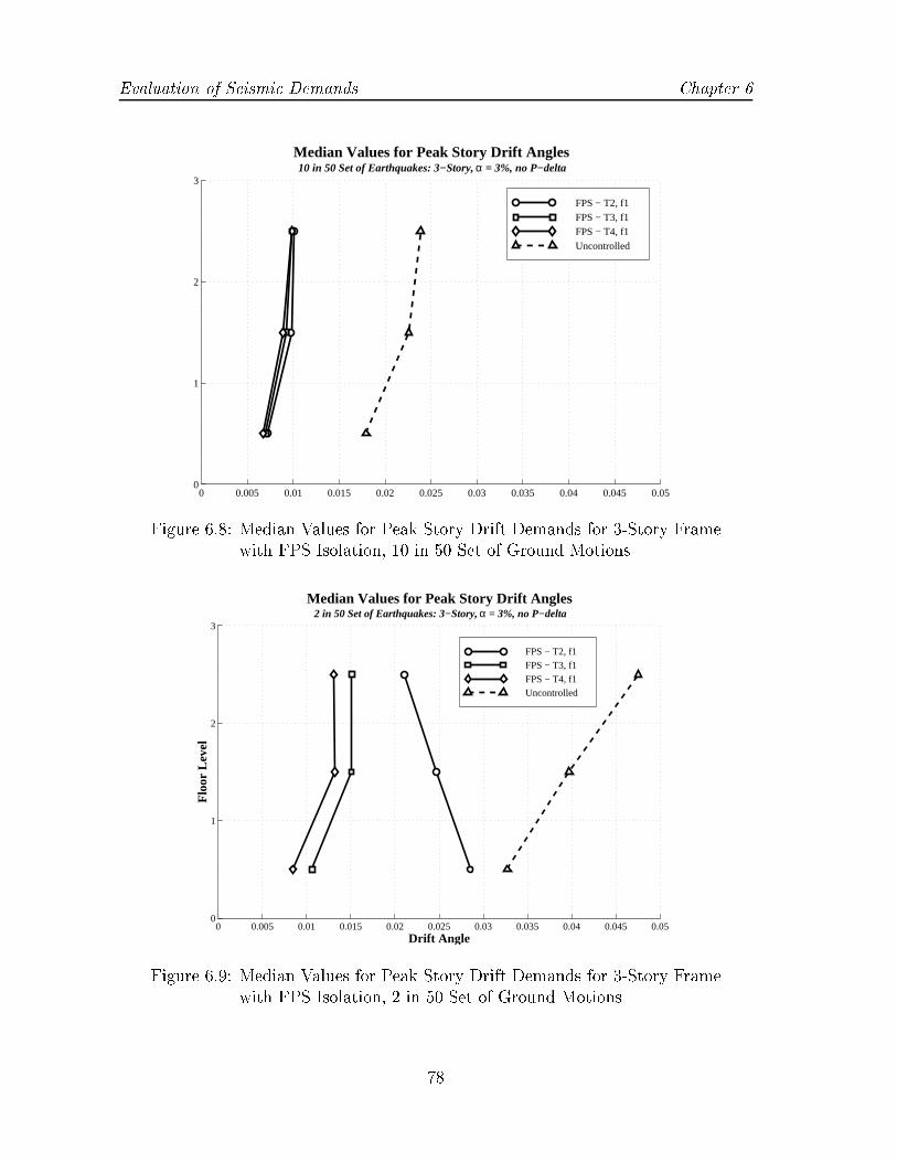
Evaluation of Seismic Demands Chapter 6
0 0.005 0.01 0.015 0.02 0.025 0.03 0.035 0.04 0.045 0.050
1
2
3
Median Values for Peak Story Drift Angles 10 in 50 Set of Earthquakes: 3−Story, α = 3%, no P−delta
FPS − T2, f1FPS − T3, f1FPS − T4, f1Uncontrolled
Figure 6.8: Median Values for Peak Story Drift Demands for 3-Story Framewith FPS Isolation, 10 in 50 Set of Ground Motions
0 0.005 0.01 0.015 0.02 0.025 0.03 0.035 0.04 0.045 0.050
1
2
3
Median Values for Peak Story Drift Angles 2 in 50 Set of Earthquakes: 3−Story, α = 3%, no P−delta
Drift Angle
Flo
or L
evel
FPS − T2, f1FPS − T3, f1FPS − T4, f1Uncontrolled
Figure 6.9: Median Values for Peak Story Drift Demands for 3-Story Framewith FPS Isolation, 2 in 50 Set of Ground Motions
78
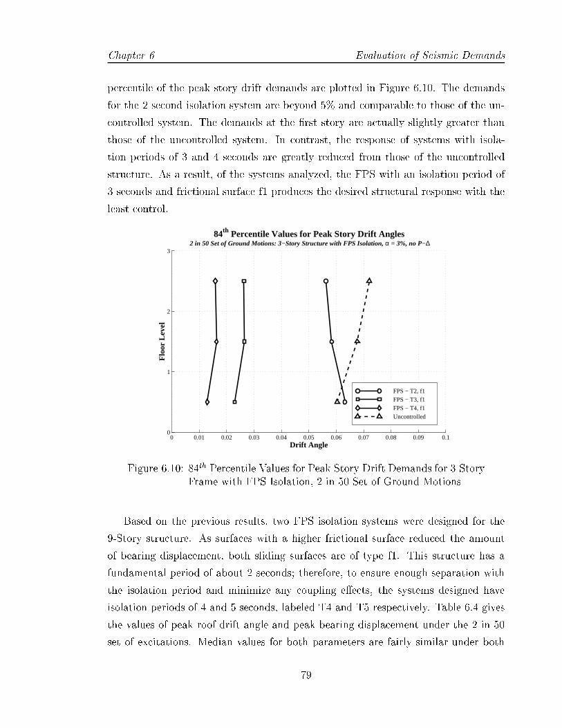
Chapter 6 Evaluation of Seismic Demands
percentile of the peak story drift demands are plotted in Figure 6.10. The demands
for the 2 second isolation system are beyond 5% and comparable to those of the un-
controlled system. The demands at the �rst story are actually slightly greater than
those of the uncontrolled system. In contrast, the response of systems with isola-
tion periods of 3 and 4 seconds are greatly reduced from those of the uncontrolled
structure. As a result, of the systems analyzed, the FPS with an isolation period of
3 seconds and frictional surface f1 produces the desired structural response with the
least control.
0 0.01 0.02 0.03 0.04 0.05 0.06 0.07 0.08 0.09 0.10
1
2
3
Drift Angle
Flo
or L
evel
84th Percentile Values for Peak Story Drift Angles 2 in 50 Set of Ground Motions: 3−Story Structure with FPS Isolation, α = 3%, no P−∆
FPS − T2, f1FPS − T3, f1FPS − T4, f1Uncontrolled
Figure 6.10: 84th Percentile Values for Peak Story Drift Demands for 3-StoryFrame with FPS Isolation, 2 in 50 Set of Ground Motions
Based on the previous results, two FPS isolation systems were designed for the
9-Story structure. As surfaces with a higher frictional surface reduced the amount
of bearing displacement, both sliding surfaces are of type f1. This structure has a
fundamental period of about 2 seconds; therefore, to ensure enough separation with
the isolation period and minimize any coupling e�ects, the systems designed have
isolation periods of 4 and 5 seconds, labeled T4 and T5 respectively. Table 6.4 gives
the values of peak roof drift angle and peak bearing displacement under the 2 in 50
set of excitations. Median values for both parameters are fairly similar under both
79
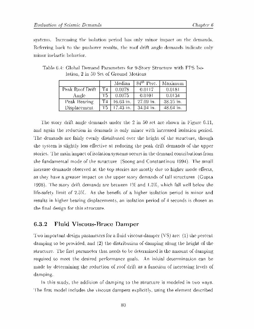
Evaluation of Seismic Demands Chapter 6
systems. Increasing the isolation period has only minor impact on the demands.
Referring back to the pushover results, the roof drift angle demands indicate only
minor inelastic behavior.
Table 6.4: Global Demand Parameters for 9-Story Structure with FPS Iso-lation, 2 in 50 Set of Ground Motions
Median 84th Perc. MaximumPeak Roof Drift
AngleT4 0.0078 0.0117 0.0181T5 0.0075 0.0101 0.0134
Peak BearingDisplacement
T4 16.63 in. 27.09 in. 38.25 in.T5 17.43 in. 34.94 in. 48.64 in.
The story drift angle demands under the 2 in 50 set are shown in Figure 6.11,
and again the reduction in demands is only minor with increased isolation period.
The demands are fairly evenly distributed over the height of the structure, though
the system is slightly less e�ective at reducing the peak drift demands of the upper
stories. The main impact of isolation systems occurs in the demand contributions from
the fundamental mode of the structure (Soong and Constantinou 1994). The small
increase demands observed at the top stories are mostly due to higher mode e�ects,
as they have a greater impact on the upper story demands of tall structures (Gupta
1998). The story drift demands are between 1% and 1.5%, which fall well below the
life-safety limit of 2.5%. As the bene�t of a higher isolation period is minor and
results in higher bearing displacements, an isolation period of 4 seconds is chosen as
the �nal design for this structure.
6.3.2 Fluid Viscous-Brace Damper
Two important design parameters for a uid viscous damper (VS) are: (1) the percent
damping to be provided, and (2) the distribution of damping along the height of the
structure. The �rst parameter that needs to be determined is the amount of damping
required to meet the desired performance goals. An initial determination can be
made by determining the reduction of roof drift as a function of increasing levels of
damping.
In this study, the addition of damping to the structure is modeled in two ways.
The �rst model includes the viscous dampers explicitly, using the element described
80
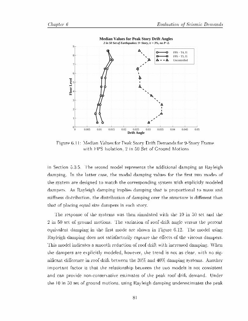
Chapter 6 Evaluation of Seismic Demands
0 0.005 0.01 0.015 0.02 0.025 0.03 0.035 0.04 0.045 0.050
1
2
3
4
5
6
7
8
9
Median Values for Peak Story Drift Angles 2 in 50 Set of Earthquakes: 9−Story, α = 3%, no P−∆
Drift Angle
Flo
or L
evel
FPS − T4, f1
FPS − T5, f1
Uncontrolled
Figure 6.11: Median Values for Peak Story Drift Demands for 9-Story Framewith FPS Isolation, 2 in 50 Set of Ground Motions
in Section 5.3.5. The second model represents the additional damping as Rayleigh
damping. In the latter case, the modal damping values for the �rst two modes of
the system are designed to match the corresponding system with explicitly modeled
dampers. As Rayleigh damping implies damping that is proportional to mass and
sti�ness distribution, the distribution of damping over the structure is di�erent than
that of placing equal size dampers in each story.
The response of the systems was then simulated with the 10 in 50 set and the
2 in 50 set of ground motions. The variation of roof drift angle versus the percent
equivalent damping in the �rst mode are shown in Figure 6.12. The model using
Rayleigh damping does not satisfactorily capture the e�ects of the viscous dampers.
This model indicates a smooth reduction of roof drift with increased damping. When
the dampers are explicitly modeled, however, the trend is not as clear, with no sig-
ni�cant di�erence in roof drift between the 30% and 40% damping systems. Another
important factor is that the relationship between the two models is not consistent
and can provide non-conservative estimates of the peak roof drift demand. Under
the 10 in 50 set of ground motions, using Rayleigh damping underestimates the peak
81

Evaluation of Seismic Demands Chapter 6
0 5 10 15 20 25 30 35 400
0.005
0.01
0.015
0.02
0.025
0.03
Percent Critical Damping
Roo
f Drif
t Ang
le
Effect of Damping on Median Peak Roof Drift Angle 3−Story Frame, α = 3%, no P−∆
VS, D1 − 2/50
Rayleigh − 2/50
VS, D1 − 10/50
Rayleigh − 10/50
Figure 6.12: Median Values for Peak Roof Drift Angle for 3-Story Frame asFunction of Percent of Critical Damping, 10 in 50 and 2 in 50Set of Ground Motions
roof drift demands. However, under the 2 in 50 set of ground motions, the Rayleigh
damping model overestimates the roof drift demand.
All three VS systems produce very similar story drift demands under the 10 in
50 ground motions (Figure 6.13). However, under the 2 in 50 set of ground motions
(Figure 6.14), the di�erences between the systems become more apparent. In both
cases, the resulting decrease in story drift demands resulting in the increase in damp-
ing from 30% to 40% is slightly less than that of increasing the e�ective damping from
20% to 30%. This behavior re ects the e�ect observed on peak roof drift demands,
shown in Figure 6.12. Also, the VS systems demonstrate a di�erent distribution of
drift demands over the height of the structure in comparison with results from the 10
in 50 set of ground motions. This di�erence results from the signi�cant yielding in
the �rst oor of the structure at this higher demand level. Though the distribution
of drift demands for all three levels of e�ective damping are fairly equivalent, slight
di�erences are apparent with increasing damping. In the system with 20% e�ective
damping, the story with the greatest drift demand is the second story, while the third
82
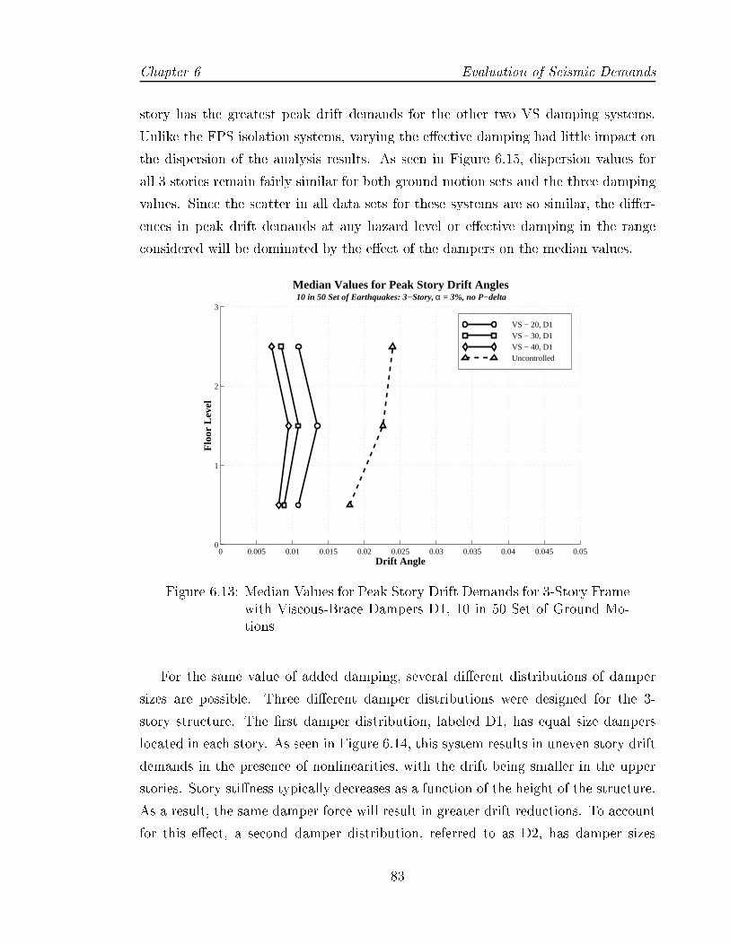
Chapter 6 Evaluation of Seismic Demands
story has the greatest peak drift demands for the other two VS damping systems.
Unlike the FPS isolation systems, varying the e�ective damping had little impact on
the dispersion of the analysis results. As seen in Figure 6.15, dispersion values for
all 3 stories remain fairly similar for both ground motion sets and the three damping
values. Since the scatter in all data sets for these systems are so similar, the di�er-
ences in peak drift demands at any hazard level or e�ective damping in the range
considered will be dominated by the e�ect of the dampers on the median values.
0 0.005 0.01 0.015 0.02 0.025 0.03 0.035 0.04 0.045 0.050
1
2
3
Median Values for Peak Story Drift Angles 10 in 50 Set of Earthquakes: 3−Story, α = 3%, no P−delta
Drift Angle
Flo
or L
evel
VS − 20, D1 VS − 30, D1 VS − 40, D1 Uncontrolled
Figure 6.13: Median Values for Peak Story Drift Demands for 3-Story Framewith Viscous-Brace Dampers D1, 10 in 50 Set of Ground Mo-tions
For the same value of added damping, several di�erent distributions of damper
sizes are possible. Three di�erent damper distributions were designed for the 3-
story structure. The �rst damper distribution, labeled D1, has equal size dampers
located in each story. As seen in Figure 6.14, this system results in uneven story drift
demands in the presence of nonlinearities, with the drift being smaller in the upper
stories. Story sti�ness typically decreases as a function of the height of the structure.
As a result, the same damper force will result in greater drift reductions. To account
for this e�ect, a second damper distribution, referred to as D2, has damper sizes
83

Evaluation of Seismic Demands Chapter 6
0 0.005 0.01 0.015 0.02 0.025 0.03 0.035 0.04 0.045 0.050
1
2
3
Median Values for Peak Story Drift Angles 2 in 50 Set of Earthquakes: 3−Story, α = 3%, no P−delta
Drift Angle
Flo
or L
evel
VS − 20, D1 VS − 30, D1 VS − 40, D1 Uncontrolled
Figure 6.14: Median Values for Peak Story Drift Demands for 3-Story Framewith Viscous-Brace Dampers D1, 2 in 50 Set of Ground Motions
0 0.1 0.2 0.3 0.4 0.5
1
2
3
Dispersion of Peak Story Drift Angles − Variation of Effective Damping LA 3−Story Structure with Evenly Distributed VS Dampers: α = 3%, no P−∆
Flo
or L
evel
Std. Deviation of the Log. of Peak Drift Angle
2/50 − V20
2/50 − V30
2/50 − V40
10/50 − V20
10/50 − V30
10/50 − V40
Figure 6.15: Dispersion of Peak Story Drift Angle for 3-Story Structure withVarying Added E�ective Damping Periods
84

Chapter 6 Evaluation of Seismic Demands
distributed proportional to an estimate of story sti�ness.
In order to estimate relative story sti�nesses, an estimate of story yield drifts is
required. An estimate for the story drift can be readily obtained if the following
simplifying assumptions are made (Krawinkler 1978; Gupta 1998):
1. The in ection points are assumed to be at the mid-heights of the columns and
midspans of the beams for structures that have no apparent strength or sti�ness
irregularities.
2. Yielding can be assumed to occur in beam elements �rst. For structures de-
signed according to strong-column/weak-beam building code criterion, this as-
sumption is reasonable.
3. Lateral de ections due to axial deformation of the columns as well as second-
order e�ects can be neglected.
In the situations where the above conditions hold, the story yield drift is not expected
to be signi�cantly di�erent between adjacent stories. Consider a typical subassembly
as shown in Figure 6.16, where in ection points are assumed to be at the mid-heights
of the columns. Assuming that the beams are the �rst elements to yield at the con-
δ
h
l/2 l/2
Ic
Ib
Figure 6.16: Beam-Column Subassembly for an Interior Column
nection, then the shear force in the columns, Vcol, can be estimated by the following:
Vcol =�M
h
0@1� dc
l
1A
=2Mpb
h
0@1� dc
l
1A
(6.1)
85
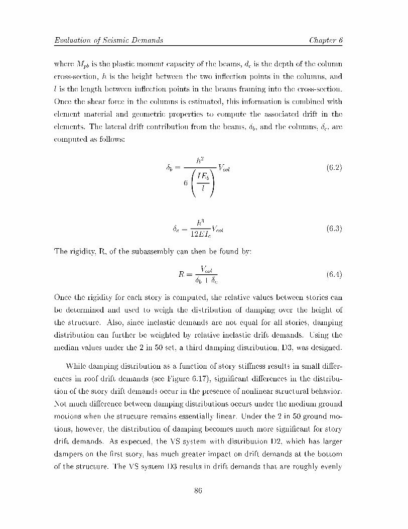
Evaluation of Seismic Demands Chapter 6
where Mpb is the plastic moment capacity of the beams, dc is the depth of the column
cross-section, h is the height between the two in ection points in the columns, and
l is the length between in ection points in the beams framing into the cross-section.
Once the shear force in the columns is estimated, this information is combined with
element material and geometric properties to compute the associated drift in the
elements. The lateral drift contribution from the beams, Æb, and the columns, Æc, are
computed as follows:
Æb =h2
6
0@IEb
l
1AVcol (6.2)
Æc =h3
12EIcVcol (6.3)
The rigidity, R, of the subassembly can then be found by:
R =Vcol
Æb + Æc(6.4)
Once the rigidity for each story is computed, the relative values between stories can
be determined and used to weigh the distribution of damping over the height of
the structure. Also, since inelastic demands are not equal for all stories, damping
distribution can further be weighted by relative inelastic drift demands. Using the
median values under the 2 in 50 set, a third damping distribution, D3, was designed.
While damping distribution as a function of story sti�ness results in small di�er-
ences in roof drift demands (see Figure 6.17), signi�cant di�erences in the distribu-
tion of the story drift demands occur in the presence of nonlinear structural behavior.
Not much di�erence between damping distributions occurs under the medium ground
motions when the structure remains essentially linear. Under the 2 in 50 ground mo-
tions, however, the distribution of damping becomes much more signi�cant for story
drift demands. As expected, the VS system with distribution D2, which has larger
dampers on the �rst story, has much greater impact on drift demands at the bottom
of the structure. The VS system D3 results in drift demands that are roughly evenly
86

Chapter 6 Evaluation of Seismic Demands
0 5 10 15 20 25 30 35 400
0.005
0.01
0.015
0.02
0.025
0.03
0.035
0.04
Percent Critical Damping
Roo
f Drif
t Ang
le
Effect of Damping Distribution on Median Peak Roof Drift Angle Variation over Damping: 3−Story Frame, α = 3%, no P−∆
D1 − 2/50
D2 − 2/50
D3 − 2/50
D1 − 10/50
D2 − 10/50
D3 − 10/50
Figure 6.17: Median Values for Peak Roof Drift Demands for 3-Story Framewith Viscous-Brace Dampers in Di�erent Distributions
distributed over the three stories. Both of these trends are also re ected in the peak
forces through the dampers, as seen in Table 6.5. These forces are on the high end
of those achievable through one damper per story.
A similar design process was adopted for the 9-story structure. The e�ect of three
di�erent damping levels, 10%, 20% and 30%, and two di�erent damping distributions,
D1 and D3 as described above, were investigated. The e�ect of variation on the
amount of damping provided is similar to that observed in the 3-Story structure, as
illustrated in Figure 6.19. Even a small amount of additional damping has a signi�cant
impact on the amount and distribution drift demands. The largest impacts are found
at the top stories, where story sti�ness and inertial mass are smaller. Redistribution
of damping, D3, results in a more even distribution of drift demands over the height
of the structure, as well as reducing the maximum peak demand over all stories, as
seen in Figure 6.20. Though not a perfectly even distribution, this approach can
provide a better starting point for an iterative design process where the goal is to
evenly distribute drift demands over the height of the structure.
87

Evaluation of Seismic Demands Chapter 6
0 0.005 0.01 0.015 0.02 0.025 0.03 0.035 0.04 0.045 0.050
1
2
3
Median Values for Peak Story Drift Angles 2 in 50 Set of Earthquakes: 3−Story, α = 3%, no P−delta
Drift Angle
Flo
or L
evel
VS − 30, D1VS − 30, D2VS − 30, D3Rayleigh 30
Figure 6.18: E�ect of Damping Distribution on Median Values for Peak StoryDrift Demands for 3-Story Frame, 2 in 50 Set of Ground Motions
Table 6.5: Median Response Properties for Viscous Dampers, 2 in 50 Set ofGround Motions
Percent ofDistribution
Peak Damper Force (kips)Critical Damping Story 1 Story 2 Story 3
20%D1 587 657 590D3 811 698 305
30%
D1 872 907 696D2 1,278 921 342D3 1,127 1,012 399
40%D1 1,103 1,085 764D3 1,425 1,151 466
88

Chapter 6 Evaluation of Seismic Demands
0 0.005 0.01 0.015 0.02 0.025 0.03 0.035 0.04 0.045 0.050
1
2
3
4
5
6
7
8
9
Median Values for Peak Story Drift Angles 2 in 50 Set of Earthquakes: 9−Story, α = 3%, no P−∆
Drift Angle
Flo
or L
evel
VS − 10, D1
VS − 20, D1
VS − 30, D1
Uncontrolled
Figure 6.19: Median Values for Peak Story Drift Demands for 9-Story Framewith Viscous-Brace Dampers D1, 2 in 50 Set of Ground Motions
0 0.005 0.01 0.015 0.02 0.025 0.03 0.035 0.04 0.045 0.050
1
2
3
4
5
6
7
8
9
Median Values for Peak Story Drift Angles for Various Damping Distributions 2 in 50 Set of Earthquakes: 9−Story, α = 3%, no P−∆
Drift Angle
Flo
or L
evel
VS − 30, D1VS − 30, D3
Figure 6.20: E�ect of Damping Distribution on Median Values for Peak StoryDrift Demands for 9-Story Frame, 2 in 50 Set of Ground Motions
89

Evaluation of Seismic Demands Chapter 6
6.3.3 Active Tendon System
Several di�erent decisions are made in the design of an active control system which
directly impact the system's ultimate performance. A detailed analysis of these con-
cerns can be found in Breneman (1999). In this investigation, only the e�ect of control
e�ort, represented by the actuator saturation level, for an active-tendon brace control
system (ATB) is investigated. For this structure, the active tendon-braces are located
in each story of the structure and designed as described in Section 4.4.3, with only a
single output variable used to represent the regulated output of story drifts. One of
the consequences of this design decision is that, since a linear combination of drifts
is used, drift values of opposite signs cancel one another during the design process.
This e�ect is discussed in detail in Breneman (1999). Two di�erent saturation levels
were speci�ed for the same control architecture and design process. The �rst system
saturates at a force of 325 kips and is referred to as the S325 system. This satura-
tion level of about 5% of the frame's seismic weight seems a realistic value for this
structure. However, in order to evaluate a system with control forces of comparable
magnitude as those of the viscous-brace system, the second system with a saturation
level of 1000 kips, labeled S1k, was also designed.
For the 10 in 50 set of ground motions, both systems reduce the story drifts, as
seen in Figure 6.21. As expected, the S1k system produces signi�cantly higher drift
reductions than the S325 system. A moderate amount of nonlinear behavior still
occurs with the S325 system, but the system is robust enough to deal with those
variations in system properties.
However, under the 2 in 50 ground motions, both ATB systems perform unsatis-
factorily, as seen in Figure 6.22. The resulting nonlinearity from these ground motions
leads to a system that is not adequately controlled. If the only concern is the reduc-
tion of the absolute maximum story drift value, then these two systems do provide a
small measure of improvement in the mean peak story drift value. The reduction in
drift of the upper story is made at the cost of increasing the drift at the lower stories.
As mentioned previously, the story sti�ness and seismic mass at the upper stories
is less than those values for the lower stories. So for the same amount of actuator
force a greater impact will be felt at the top stories. Since the controller weights
all story drifts equally, the �rst story drift is sacri�ced to achieve improvements in
90
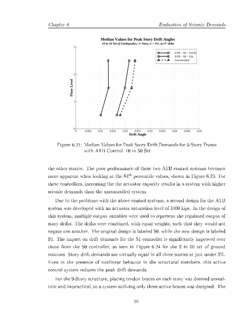
Chapter 6 Evaluation of Seismic Demands
0 0.005 0.01 0.015 0.02 0.025 0.03 0.035 0.04 0.045 0.050
1
2
3
Median Values for Peak Story Drift Angles 10 in 50 Set of Earthquakes: 3−Story, α = 3%, no P−delta
Drift Angle
Flo
or L
evel
ATB − S0 − S325k ATB − S0 − S1k Uncontrolled
Figure 6.21: Median Values for Peak Story Drift Demands for 3-Story Framewith ATB Control, 10 in 50 Set
the other stories. The poor performance of these two ATB control systems becomes
more apparent when looking at the 84th percentile values, shown in Figure 6.23. For
these controllers, increasing the the actuator capacity results in a system with higher
seismic demands than the uncontrolled system.
Due to the problems with the above control systems, a second design for the ATB
system was developed with an actuator saturation level of 1000 kips. In the design of
this system, multiple output variables were used to represent the regulated output of
story drifts. The drifts were combined, with equal weights, such that they would not
negate one another. The original design is labeled S0, while the new design is labeled
S1. The impact on drift demands for the S1 controller is signi�cantly improved over
those from the S0 controller, as seen in Figure 6.24 for the 2 in 50 set of ground
motions. Story drift demands are virtually equal in all three stories at just under 3%.
Even in the presence of nonlinear behavior in the structural members, this active
control system reduces the peak drift demands.
For the 9-Story structure, placing tendon braces on each story was deemed unreal-
istic and impractical, so a system utilizing only three active braces was designed. The
91
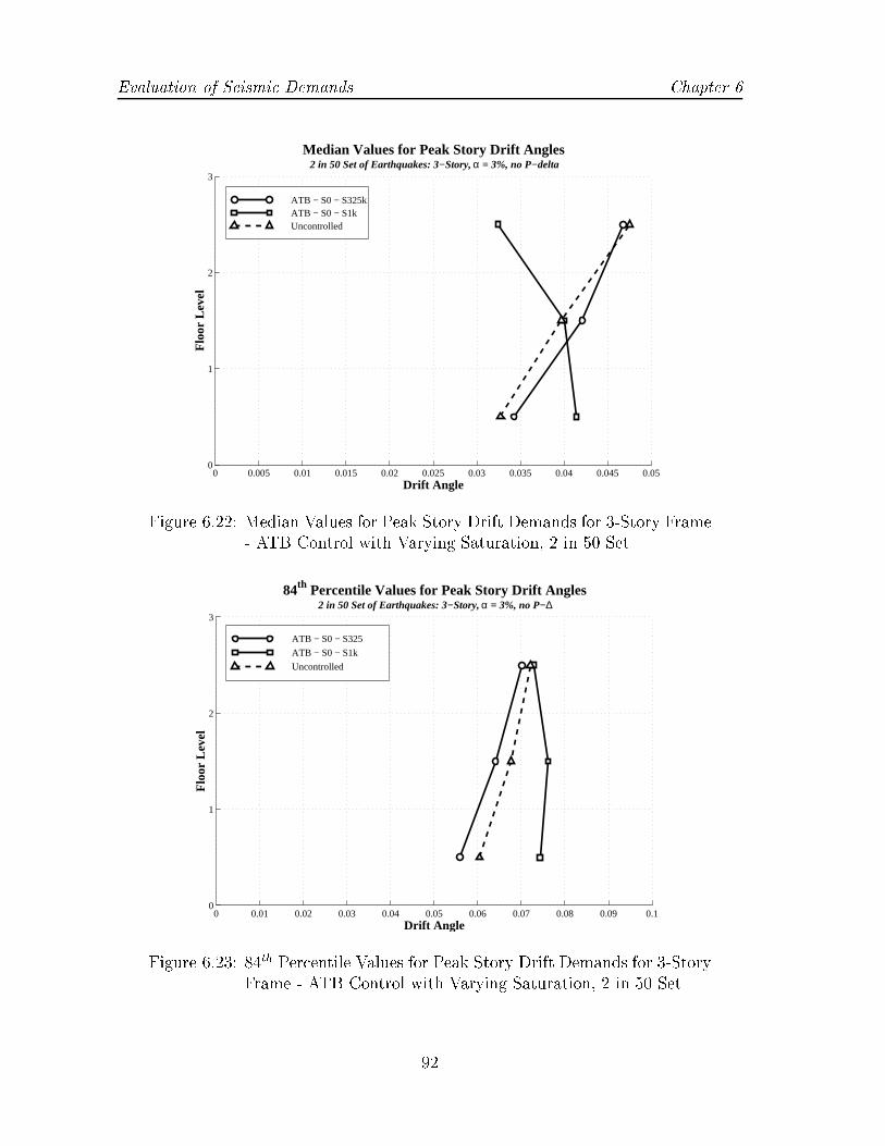
Evaluation of Seismic Demands Chapter 6
0 0.005 0.01 0.015 0.02 0.025 0.03 0.035 0.04 0.045 0.050
1
2
3
Median Values for Peak Story Drift Angles 2 in 50 Set of Earthquakes: 3−Story, α = 3%, no P−delta
Drift Angle
Flo
or L
evel
ATB − S0 − S325k ATB − S0 − S1k Uncontrolled
Figure 6.22: Median Values for Peak Story Drift Demands for 3-Story Frame- ATB Control with Varying Saturation, 2 in 50 Set
0 0.01 0.02 0.03 0.04 0.05 0.06 0.07 0.08 0.09 0.10
1
2
3
Drift Angle
Flo
or L
evel
84th Percentile Values for Peak Story Drift Angles 2 in 50 Set of Earthquakes: 3−Story, α = 3%, no P−∆
ATB − S0 − S325
ATB − S0 − S1k
Uncontrolled
Figure 6.23: 84th Percentile Values for Peak Story Drift Demands for 3-StoryFrame - ATB Control with Varying Saturation, 2 in 50 Set
92

Chapter 6 Evaluation of Seismic Demands
0 0.005 0.01 0.015 0.02 0.025 0.03 0.035 0.04 0.045 0.050
1
2
3
Median Values for Peak Story Drift Angles 2 in 50 Set of Earthquakes: 3−Story with ATB, α = 3%, no P−∆
Drift Angle
Flo
or L
evel
ATB − S0 − A1k
ATB − S1 − S1k
Uncontrolled
Figure 6.24: Median Values for Peak Story Drift Demands for 3-Story Framewith ATB Control, Variation in Design, 2 in 50 Set
0 0.1 0.2 0.3 0.4 0.5 0.6 0.7 0.8
1
2
3
Dispersion of Peak Story Drift Angles − Different Control Design LA 3−Story Structure with ATB System, Saturation 1k: α = 3%, no P−∆
Flo
or L
evel
Std. Deviation of the Log. of Peak Drift Angle
2/50 − S0
2/50 − S1
10/50 − S0
10/50 − S1
Figure 6.25: Dispersion of Peak Story Drift Angle for 3-Story Structure withATB Systems of Di�erent Controlled Outputs
93
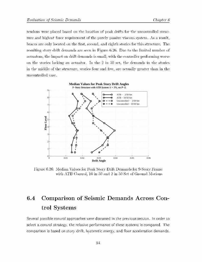
Evaluation of Seismic Demands Chapter 6
tendons were placed based on the location of peak drifts for the uncontrolled struc-
ture and highest force requirement of the purely passive viscous system. As a result,
braces are only located on the �rst, second, and eighth stories for this structure. The
resulting story drift demands are seen in Figure 6.26. Due to the limited number of
actuators, the impact on drift demands is small, with the controller performing worse
on the stories lacking an actuator. In the 2 in 50 set, the demands in the stories
in the middle of the structure, stories four and �ve, are actually greater than in the
uncontrolled case.
0 0.01 0.02 0.03 0.04 0.05 0.060
1
2
3
4
5
6
7
8
9
Median Values for Peak Story Drift Angles 9−Story Structure with ATB System: α = 3%, no P−∆
Drift Angle
Flo
or L
evel
ATB − 2/50 Set ATB − 10/50 Set Uncontrolled − 2/50 SetUncontrolled − 10/50 Set
Figure 6.26: Median Values for Peak Story Drift Demands for 9-Story Framewith ATB Control, 10 in 50 and 2 in 50 Set of Ground Motions
6.4 Comparison of Seismic Demands Across Con-
trol Systems
Several possible control approaches were discussed in the previous section. In order to
select a control strategy, the relative performance of these systems is compared. The
comparison is based on story drift, hysteretic energy, and oor acceleration demands.
94

Chapter 6 Evaluation of Seismic Demands
As discussed earlier, story drift angles and hysteretic energy demands provide an
indication of structural damage in steel moment resisting frames, while oor acceler-
ations are used as an indication of the content and acceleration-sensitive nonstructural
damage.
6.4.1 Deformation Demands
A wide consensus exists in the earthquake engineering community that for moment-
resisting frames the interstory drift demand, expressed in terms of the interstory drift
angle, is the best indicator of expected damage. As a global parameter, interstory drift
is much more appropriate than the roof drift angle because in individual stories it may
exceed the latter by a factor of two or more (Krawinkler and Gupta 1998). The use
of story substructures permits also the estimation of element force and deformation
demands from the story drift angle.
As a representative value, the median (exponent of the average value of the log of
the data) is selected. The control systems selected for comparison with the 3-Story
structure are: 1) VS with 30% damping and distribution D1, 2) FPS isolation with
isolation period of 3 seconds and frictional surface f1, and 3) ATB design S1 with
saturation level of 1000 kips. The values suggested for peak and residual story drift
angles in FEMA 273, which are listed in Table 2.1, can be used as one set of guidelines
by which performance of a SMRF structure may be judged.
The maximum story drifts over the height of the structure (maximum drift in
any story for a given ground motion) for each system are shown in Figures 6.27
through 6.29. The �gures show the 20 data points corresponding to the 20 records
in each set; the median value for the responses are shown by the solid dash mark2.
Results from the 50 in 50 set of ground motions, shown in Figure 6.27 indicate that
for a short return period the control systems can reduce the seismic demands by
nearly 50%. For this structure, the median response moves to below the immediate-
occupancy level for all 3 types of control strategies. Only a few records drive the
structure above the immediate-occupancy level, and only one beyond the life-safety
2Note that the median values indicated are the median values of the maximum peak drifts overthe height of the structure over the 20 individual ground motions. These results are not the sameas the maximum of the median individual story peak drift values, which are plotted in other �gures
95

Evaluation of Seismic Demands Chapter 6
Uncontrolled VS − 30, D1 FPS − T3, f1 ATB − S1k0
0.01
0.02
0.03
0.04
0.05
Drif
t Ang
le
Maximum Story Drift Angles 50 in 50 Set of Earthquakes: 3−Story, α = 3%, no P−delta
Figure 6.27: Maximum Values for Peak Story Drift Demands for 3-StoryFrame, 50 in 50 Set of Ground Motions
Uncontrolled VS − 30, D1 FPS − T3, f1 ATB − S1k0
0.005
0.01
0.015
0.02
0.025
0.03
0.035
0.04
0.045
0.05
Drif
t Ang
le
Maximum Story Drift Angles 10 in 50 Set of Earthquakes: 3−Story, α = 3%, no P−delta
Figure 6.28: Maximum Peak Story Drift Demands for 3-Story Frame, 10 in50 Set of Ground Motions
96

Chapter 6 Evaluation of Seismic Demands
limit in the uncontrolled system. Though the lowest median value for peak story drift
occurs with the viscous system, the scatter in the response is lowest in the presence of
the isolation system. In the 10 in 50 set, while the median uncontrolled response lies
just below the life-safety limit, several records push the uncontrolled response between
the life-safety and collapse-prevention limits, as seen in Figure 6.28. However, the ap-
plication of control reduces both the median structural response as well as its scatter.
The median response of the passive systems, while above the immediate-occupancy
limit, falls just at the linear limit of this structure, with the median response of the
ATB system just above those values. All records have responses below the life-safety
limit after the application of control.
Uncontrolled VS − 30, D1 FPS − T3, f1 ATB − S1k0
0.01
0.02
0.03
0.04
0.05
0.06
0.07
0.08
0.09
0.1
0.11
0.12
Drif
t Ang
le
Maximum Story Drift Angles 2 in 50 Set of Earthquakes: 3−Story, α = 3%, no P−delta
Figure 6.29: Maximum Peak Story Drift Demands for 3-Story Frame, 2 in50 Set of Ground Motions
The results from the 2 in 50 set of ground motions, shown in Figure 6.29, indicate
a median response for the uncontrolled systems just under the collapse prevention
limit and great scattering in the response. The original system response contains
clear outliers with story drift demands exceeding 10% drift, which are unsustainable
by the physical frame system of the SMRF and are not present in any of the controlled
systems. The ATB control system performs better under these excitations, both in
97
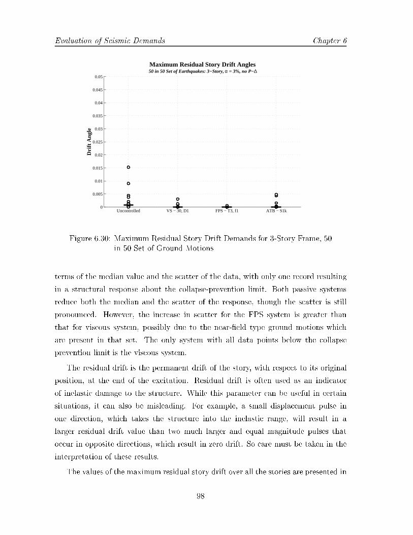
Evaluation of Seismic Demands Chapter 6
Uncontrolled VS − 30, D1 FPS − T3, f1 ATB − S1k0
0.005
0.01
0.015
0.02
0.025
0.03
0.035
0.04
0.045
0.05
Drif
t Ang
le
Maximum Residual Story Drift Angles 50 in 50 Set of Earthquakes: 3−Story, α = 3%, no P−∆
Figure 6.30: Maximum Residual Story Drift Demands for 3-Story Frame, 50in 50 Set of Ground Motions
terms of the median value and the scatter of the data, with only one record resulting
in a structural response about the collapse-prevention limit. Both passive systems
reduce both the median and the scatter of the response, though the scatter is still
pronounced. However, the increase in scatter for the FPS system is greater than
that for viscous system, possibly due to the near-�eld type ground motions which
are present in that set. The only system with all data points below the collapse
prevention limit is the viscous system.
The residual drift is the permanent drift of the story, with respect to its original
position, at the end of the excitation. Residual drift is often used as an indicator
of inelastic damage to the structure. While this parameter can be useful in certain
situations, it can also be misleading. For example, a small displacement pulse in
one direction, which takes the structure into the inelastic range, will result in a
larger residual drift value than two much larger and equal magnitude pulses that
occur in opposite directions, which result in zero drift. So care must be taken in the
interpretation of these results.
The values of the maximum residual story drift over all the stories are presented in
98

Chapter 6 Evaluation of Seismic Demands
Uncontrolled VS − 30, D1 FPS − T3, f1 ATB − S1k0
0.005
0.01
0.015
0.02
0.025
0.03
0.035
0.04
0.045
0.05
Drif
t Ang
le
Maximum Residual Story Drift Angles 10 in 50 Set of Earthquakes: 3−Story, α = 3%, no P−∆
Figure 6.31: Maximum Residual Story Drift Demands for 3-Story Frame, 10in 50 Set of Ground Motions
Uncontrolled VS − 30, D1 FPS − T3, f1 ATB − S1k0
0.01
0.02
0.03
0.04
0.05
0.06
0.07
0.08
Drif
t Ang
le
Maximum Residual Story Drift Angles 2 in 50 Set of Earthquakes: 3−Story, α = 3%, no P−∆
Figure 6.32: Maximum Residual Story Drift Demands for 3-Story Frame, 2in 50 Set of Ground Motions
99
Evaluation of Seismic Demands Chapter 6
Figures 6.30 through 6.32, with the median value for each system indicated by a solid
horizontal line. Results from the 50 in 50 set of ground motion have median values
that are fairly close to zero for all systems, though the median values for the controlled
systems are lower than the uncontrolled system. Only one case corresponding to the
uncontrolled system is beyond the life-safety limit. The addition of control reduces the
scatter, especially for the isolation system. Under the 10 in 50 set of ground motions,
the scatter in the results increases signi�cantly for all systems. Outlier values are
apparent for all systems. Three cases in the uncontrolled system and one with the
ATB control are beyond the life-safety limit. Median values in the 2 in 50 set of ground
motions are below the life-safety limit for the uncontrolled system and the two passive
systems. However, the median value for the ATB controlled system is greater than
that of the uncontrolled structure. This example illustrates the incomplete nature
of the information given by the residual drift. In several ground motions, the use
of the ATB control is e�ective at reducing the repeated excursions into the inelastic
range relative to the uncontrolled case. As a results, in these cases the addition of
control appears to increase damage, when in reality the control system is reducing
the inelastic damage to the structural members. A comparison of the dissipated
hysteretic energy, which is discussed in Section 6.4.2, con�rms this fact.
Peak story drift demand over the height of the structure is not suÆcient to fully
understand the demands on the structural system. One must also evaluate the dis-
tribution of drift demands over the height of the structure. In the 50 in 50 set of
ground motions, shown in Figure 6.33, the median values of drift demands remain
fairly constant over the height of the structure. The largest drift ratio occurs at the
top story except for the viscous system, where the largest drift ratio occurs in the
second story. These same trends can be observed for the median values of the 10 in
50 set of ground motions, shown in Figure 6.35. However, the relative placement of
the demand curves for each system changes. In both cases, all three control strate-
gies reduce the story drift demands over the entire height of the structure. In the
50 in 50 set of ground motions, the viscous control system results in the lowest drift
demands. Under the stronger ground motions of the 10 in 50 set, the FPS isolation
system becomes more e�ective at reducing story drift demands. The isolation system
only starts to become e�ective once the base shear reaches the sliding force of the
bearing. As a result, this system is not as e�ective at low level ground motions. The
100

Chapter 6 Evaluation of Seismic Demands
ATB system has comparable drift demands with the passive system. The di�erences
between systems becomes more pronounced at the 84th percentile values, though the
same trends occur.
Under the 2 in 50 set of ground motions, signi�cant nonlinearities occur in the
controlled systems. Furthermore, the di�erences between control systems becomes
more pronounced, as seem in Figure 6.37. While the FPS isolation system results
in the lowest median drift demands, the e�ect of higher scatter can be seen when
comparing the median and the 84th percentile values. In comparison, the results for
the viscous system display less scatter. The ATB system has drift demands which are
higher than both passive systems, though signi�cantly reduced from the uncontrolled
case. Again the 84th percentile values indicate drift demands which increase more
than those for the viscous system. However, for all controlled systems these values
are well below the collapse prevention limit. Since the placement of the actuators
and their saturation level were designed to provide a comparable system between the
ATB and VS controller, the only di�erence lies in the control strategy and not the
physical limitations of the systems.
Care must be taken not to assume that control strategies which reduce statistical
values for the ground motion sets will reduce demands for all individual excitations. In
a motion-by-motion comparison, occasionally both active and passive control system
do make performance worse. For this structure and sets of ground motions, the FPS
isolation system always reduced roof and story drift angles. The same is not true for
the VS and ATB system, as seen in Table 6.6. In the VS controlled system, three
ground motions within the 2 in 50 set led to slightly higher drifts in the �rst story.
Similarly, two ground motions in the 2 in 50 set increase peak drift angles for both
�rst and second stories with the ATB control system.
Results for the 9-story frame story drift demands are given in Figures 6.41 and 6.44.
When comparing the e�ect of the ATB system, consideration must be given to the
fact that this system only has three actuators located on the �rst, second, and eighth
stories. The viscous system, in contrast, has dampers located on each story. In the
10 in 50 set of excitations, all control systems produce reductions in the story drift
demands. The passive systems have the most signi�cant reduction in drifts, with
comparable performance. The FPS isolation system proves to be more e�ective in
the lower structures, while the VS system is more e�ective in the upper stories. The
101

Evaluation of Seismic Demands Chapter 6
0 0.005 0.01 0.015 0.02 0.025 0.03 0.035 0.04 0.045 0.050
1
2
3
Median Values for Peak Story Drift Angles 50 in 50 Set of Earthquakes: 3−Story, α = 3%, no P−delta
Drift Angle
Flo
or L
evel
Uncontrolled
Viscous − 30, D1
FPS − T3, f1
ATB − 1000k
Figure 6.33: Median Peak Story Drift Demands for 3-Story Frame, 50 in 50Set of Earthquakes
0 0.005 0.01 0.015 0.02 0.025 0.03 0.035 0.04 0.045 0.050
1
2
3
Drift Angle
Flo
or L
evel
84th Percentile Values for Peak Story Drift Angles 50 in 50 Set of Earthquakes: 3−Story, α = 3%, no P−delta
Uncontrolled
Viscous − 30, D1
FPS − T3, f1
ATB − 1000k
Figure 6.34: 84th Percentile Values for Peak Story Drift Demands for 3-StoryFrame, 50 in 50 Set of Earthquakes
102
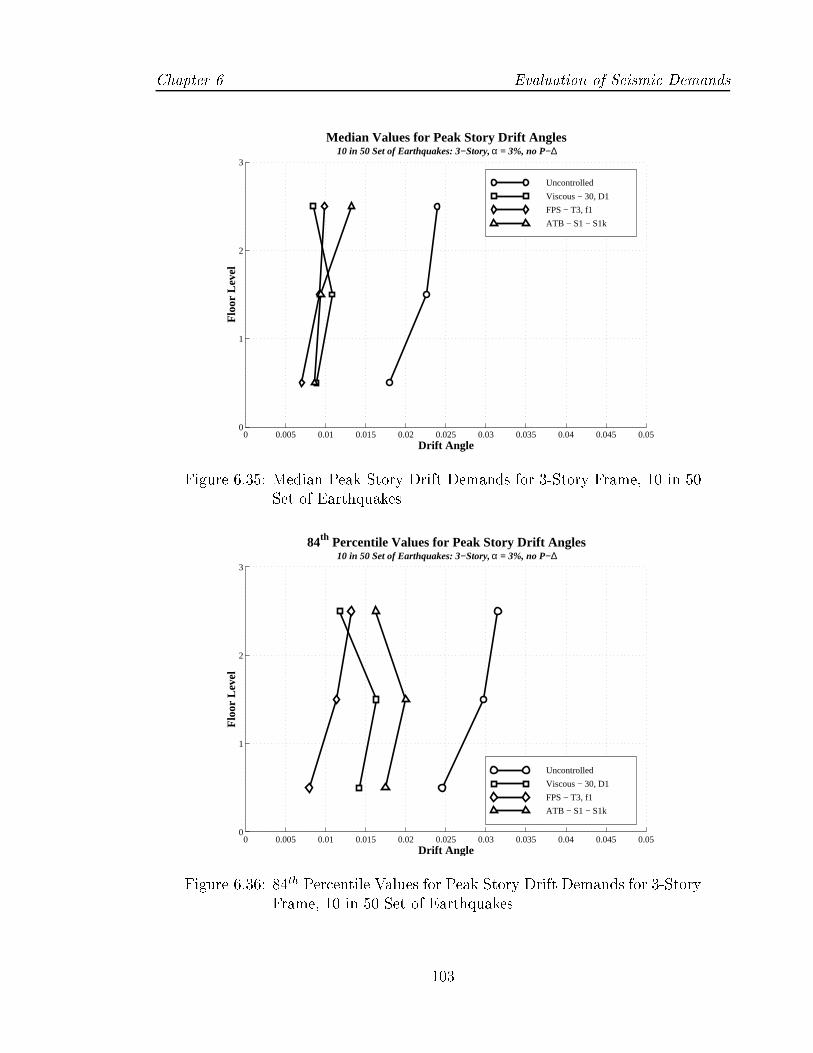
Chapter 6 Evaluation of Seismic Demands
0 0.005 0.01 0.015 0.02 0.025 0.03 0.035 0.04 0.045 0.050
1
2
3
Median Values for Peak Story Drift Angles 10 in 50 Set of Earthquakes: 3−Story, α = 3%, no P−∆
Drift Angle
Flo
or L
evel
Uncontrolled
Viscous − 30, D1
FPS − T3, f1
ATB − S1 − S1k
Figure 6.35: Median Peak Story Drift Demands for 3-Story Frame, 10 in 50Set of Earthquakes
0 0.005 0.01 0.015 0.02 0.025 0.03 0.035 0.04 0.045 0.050
1
2
3
Drift Angle
Flo
or L
evel
84th Percentile Values for Peak Story Drift Angles 10 in 50 Set of Earthquakes: 3−Story, α = 3%, no P−∆
Uncontrolled
Viscous − 30, D1
FPS − T3, f1
ATB − S1 − S1k
Figure 6.36: 84th Percentile Values for Peak Story Drift Demands for 3-StoryFrame, 10 in 50 Set of Earthquakes
103

Evaluation of Seismic Demands Chapter 6
0 0.005 0.01 0.015 0.02 0.025 0.03 0.035 0.04 0.045 0.050
1
2
3
Median Values for Peak Story Drift Angles 2 in 50 Set of Earthquakes: 3−Story, α = 3%, no P−delta
Drift Angle
Flo
or L
evel
Uncontrolled
Viscous − 30, D1
FPS − T3, f1
ATB − 1000k
Figure 6.37: Median Peak Story Drift Demands for 3-Story Frame, 2 in 50Set of Earthquakes
0 0.01 0.02 0.03 0.04 0.05 0.06 0.07 0.08 0.09 0.10
1
2
3
Drift Angle
Flo
or L
evel
84th Percentile Values for Peak Story Drift Angles 2 in 50 Set of Earthquakes: 3−Story, α = 3%, no P−delta
Uncontrolled
Viscous − 30, D1
FPS − T3, f1
ATB − 1000k
Figure 6.38: 84th Percentile Values for Peak Story Drift Demands for 3-StoryFrame, 2 in 50 Set of Earthquakes
104

Chapter 6 Evaluation of Seismic Demands
Table 6.6: Increases in Story Drift Demands for 3-Story Structure due toAdditional Control, 2 in 50 Set of Ground Motions
Ground Motion Story Percent Increase
VS 30
la41 1 9.1la42 1 12.0la52 1 6.6
ATB
la41 1 9.5la41 2 16.8la52 1 9.8la52 2 2.5
impact of the active system is minor, with some stories showing almost no improve-
ment. In the 2 in 50 set, the two passive systems again show signi�cant reductions
in drift demands, with all story drifts below the life-safety limit of 2.5%. Again, the
FPS isolation has the lowest drift demands for the lower stories, while the VS system
has the lowest values for the upper stories. On average, however, the FPS isolation
performs better, with its worst story drift demand below that for the VS system. In
contrast, the ATB is only e�ective in reducing the demands near the location of its
actuators. The drift demands in the fourth and �fth stories actually increases when
compared to the original uncontrolled structure.
In order to allow for a better comparison between the e�ects of the ATB and VS
systems, two additional VS systems were designed for this structure. The �rst system,
VS 30 - 3 brace, utilizes the same size dampers as in the viscous system with 30%
damping evenly distributed (VS 30, D1). This design results in a controlled system
with approximately 10% damping in the �rst mode of the structure. The second
damping system uses that 10% damping evenly over the height of the structure, VS
10, D1. The resulting drift demands are shown in Figure 6.45. When only the 3
braces are utilized, the VS system also increases the drift demands of the middle
stories. The additional dampers cause those stories to be more diÆcult to deform.
As a result, the seismic demands are redistributed to locations which are easier to
deform. However, the VS system still performs better than the ATB system when
comparing the maximum value of story drift over the all stories. In comparison, using
the damping evenly throughout the structure results in reduction of drift demands
for all stories.
105

Evaluation of Seismic Demands Chapter 6
0 0.005 0.01 0.015 0.02 0.025 0.03 0.035 0.04 0.045 0.05
1
2
3
4
5
6
7
8
9
Median Values for Peak Story Drift Angles 50 in 50 Set of Earthquakes: 3−Story, α = 3%, no P−delta
Drift Angle
Flo
or L
evel
Uncontrolled
Viscous − 30, D1
FPS − T4, f1
ATB − S1k
Figure 6.39: Median Peak Story Drift Demands for 9-Story Frame, 10 in 50Set of Earthquakes
0 0.005 0.01 0.015 0.02 0.025 0.03 0.035 0.04 0.045 0.050
1
2
3
4
5
6
7
8
9
Drift Angle
Flo
or L
evel
84th Percentile Values for Peak Story Drift Angles 50 in 50 Set of Earthquakes: 3−Story, α = 3%, no P−delta
Uncontrolled
Viscous − 30, D1
FPS − T3, f1
ATB − S1k
Figure 6.40: 84th Percentile Values for Peak Story Drift Demands for 9-StoryFrame, 10 in 50 Set of Earthquakes
106
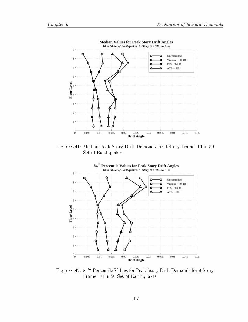
Chapter 6 Evaluation of Seismic Demands
0 0.005 0.01 0.015 0.02 0.025 0.03 0.035 0.04 0.045 0.05
1
2
3
4
5
6
7
8
9
Median Values for Peak Story Drift Angles 10 in 50 Set of Earthquakes: 9−Story, α = 3%, no P−∆
Drift Angle
Flo
or L
evel
Uncontrolled
Viscous − 30, D1
FPS − T4, f1
ATB − S1k
Figure 6.41: Median Peak Story Drift Demands for 9-Story Frame, 10 in 50Set of Earthquakes
0 0.005 0.01 0.015 0.02 0.025 0.03 0.035 0.04 0.045 0.050
1
2
3
4
5
6
7
8
9
Drift Angle
Flo
or L
evel
84th Percentile Values for Peak Story Drift Angles 10 in 50 Set of Earthquakes: 9−Story, α = 3%, no P−∆
Uncontrolled
Viscous − 30, D1
FPS − T3, f1
ATB − S1k
Figure 6.42: 84th Percentile Values for Peak Story Drift Demands for 9-StoryFrame, 10 in 50 Set of Earthquakes
107

Evaluation of Seismic Demands Chapter 6
0 0.005 0.01 0.015 0.02 0.025 0.03 0.035 0.04 0.045 0.05
1
2
3
4
5
6
7
8
9
Median Values for Peak Story Drift Angles 2 in 50 Set of Earthquakes: 9−Story, α = 3%, no P−∆
Drift Angle
Flo
or L
evel
Uncontrolled
Viscous − 30, D1
FPS − T4, f1
ATB − S1k
Figure 6.43: 84th Percentile Values for Peak Story Drift Demands for 9-StoryFrame, 2 in 50 Set of Earthquakes
0 0.01 0.02 0.03 0.04 0.05 0.060
1
2
3
4
5
6
7
8
9
Drift Angle
Flo
or L
evel
84th Percentile Values for Peak Story Drift Angles 2 in 50 Set of Earthquakes: 9−Story, α = 3%, no P−∆
Uncontrolled
Viscous − 30, D1
FPS − T3, f1
ATB − S1k
Figure 6.44: 84th Percentile Values for Peak Story Drift Demands for 9-StoryFrame, 2 in 50 Set of Earthquakes
108

Chapter 6 Evaluation of Seismic Demands
0 0.005 0.01 0.015 0.02 0.025 0.03 0.035 0.04 0.045 0.05
1
2
3
4
5
6
7
8
9
Median Values for Peak Story Drift Angles 2 in 50 Set of Earthquakes: 9−Story, α = 3%, no P−∆
Drift Angle
Flo
or L
evel
Uncontrolled VS 30: 3−brace VS 10 − D1: all storiesATB − S1k
Figure 6.45: Comparison of Maximum Peak Story Drift Demands for VS andATB Control for 9-Story Structure
6.4.2 Hysteretic Energy Demands
While peak interstory drift provides a good indication of performance, the resulting
information is incomplete as it does not take into account the cumulative damage to
the structure. Experimental investigations have demonstrated that structural dam-
age is a function of both peak as well as cumulative values. As normalized hysteretic
energy (NHE) provides a good indication of cumulative damage in steel structures,
median values of NHE are compared for control systems for each set of ground mo-
tions. Normalization of the hysteretic energy values of each element is performed by
normalizing by that elements elastic energy capacity, Ee, given by:
Ee = Mp �p =M2
p l
6EI(6.5)
where Mp is the plastic moment capacity, l is the member length, E is the modulus
of elasticity, and I is the moment of inertia.
The plots give values of the cumulative NHE dissipated by the frame members
109
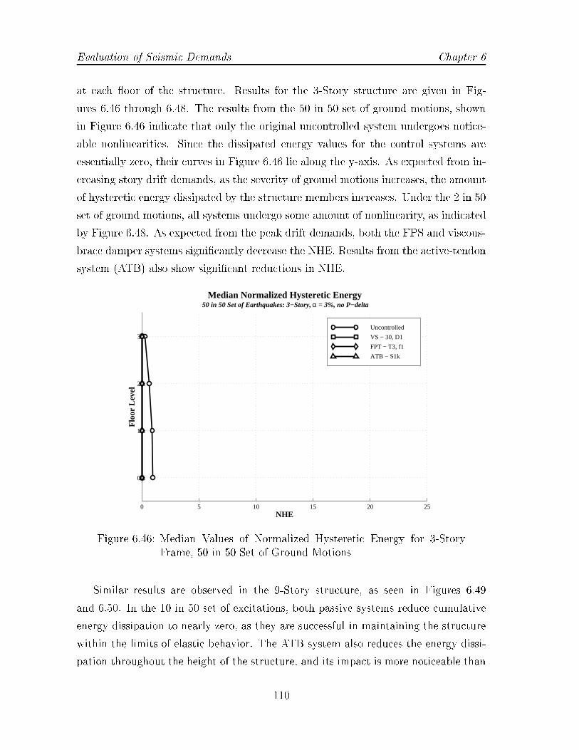
Evaluation of Seismic Demands Chapter 6
at each oor of the structure. Results for the 3-Story structure are given in Fig-
ures 6.46 through 6.48. The results from the 50 in 50 set of ground motions, shown
in Figure 6.46 indicate that only the original uncontrolled system undergoes notice-
able nonlinearities. Since the dissipated energy values for the control systems are
essentially zero, their curves in Figure 6.46 lie along the y-axis. As expected from in-
creasing story drift demands, as the severity of ground motions increases, the amount
of hysteretic energy dissipated by the structure members increases. Under the 2 in 50
set of ground motions, all systems undergo some amount of nonlinearity, as indicated
by Figure 6.48. As expected from the peak drift demands, both the FPS and viscous-
brace damper systems signi�cantly decrease the NHE. Results from the active-tendon
system (ATB) also show signi�cant reductions in NHE.
0 5 10 15 20 25
0
1
2
3
Median Normalized Hysteretic Energy 50 in 50 Set of Earthquakes: 3−Story, α = 3%, no P−delta
NHE
Flo
or L
evel
Uncontrolled
VS − 30, D1
FPT − T3, f1
ATB − S1k
Figure 6.46: Median Values of Normalized Hysteretic Energy for 3-StoryFrame, 50 in 50 Set of Ground Motions
Similar results are observed in the 9-Story structure, as seen in Figures 6.49
and 6.50. In the 10 in 50 set of excitations, both passive systems reduce cumulative
energy dissipation to nearly zero, as they are successful in maintaining the structure
within the limits of elastic behavior. The ATB system also reduces the energy dissi-
pation throughout the height of the structure, and its impact is more noticeable than
110

Chapter 6 Evaluation of Seismic Demands
0 5 10 15 20 25
0
1
2
3
Median Normalized Hysteretic Energy 10 in 50 Set of Earthquakes: 3−Story, α = 3%, no P−delta
NHE
Flo
or L
evel
Uncontrolled
VS − 30, D1
FPT − T3, f1
ATB − S1k
Figure 6.47: Median Values of Normalized Hysteretic Energy for 3-StoryFrame, 10 in 50 Set of Ground Motions
0 5 10 15 20 25
0
1
2
3
Median Normalized Hysteretic Energy 2 in 50 Set of Earthquakes: 3−Story, α = 3%, no P−delta
NHE
Flo
or L
evel
Uncontrolled
VS − 30, D1
FPT − T3, f1
ATB − S1k
Figure 6.48: Median Values of Normalized Hysteretic Energy for 3-StoryFrame, 2 in 50 Set of Ground Motions
111
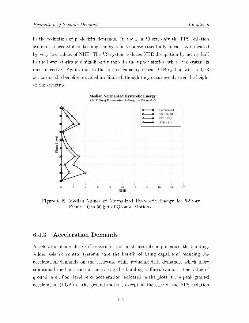
Evaluation of Seismic Demands Chapter 6
in the reduction of peak drift demands. In the 2 in 50 set, only the FPS isolation
system is successful at keeping the system response essentially linear, as indicated
by very low values of NHE. The VS system reduces NHE dissipation by nearly half
in the lower stories and signi�cantly more in the upper stories, where the system is
most e�ective. Again, due to the limited capacity of the ATB system with only 3
actuators, the bene�ts provided are limited, though they occur evenly over the height
of the structure.
0 2 4 6 8 10 12 14 16 18 20
0
1
2
3
4
5
6
7
8
9
Median Normalized Hysteretic Energy 2 in 50 Set of Earthquakes: 9−Story, α = 3%, no P−∆
NHE
Flo
or L
evel
Uncontrolled
VS − 30, D1
FPT − T3, f1
ATB − S1k
Figure 6.49: Median Values of Normalized Hysteretic Energy for 9-StoryFrame, 10 in 50 Set of Ground Motions
6.4.3 Acceleration Demands
Acceleration demands are of concern for the nonstructural components of the building.
Added seismic control systems have the bene�t of being capable of reducing the
acceleration demands on the structure while reducing drift demands, which more
traditional methods such as increasing the building sti�ness cannot. The value of
ground level, oor level zero, acceleration indicated in the plots is the peak ground
acceleration (PGA) of the ground motion, except in the case of the FPS isolation
112

Chapter 6 Evaluation of Seismic Demands
0 2 4 6 8 10 12 14 16 18 20
0
1
2
3
4
5
6
7
8
9
Median Normalized Hysteretic Energy 2 in 50 Set of Earthquakes: 9−Story, α = 3%, no P−∆
NHE
Flo
or L
evel
Uncontrolled
VS − 30, D1
FPT − T3, f1
ATB − S1k
Figure 6.50: Median Values of Normalized Hysteretic Energy for 9-StoryFrame, 2 in 50 Set of Ground Motions
system. In that system, the acceleration reported is that observed immediately above
the isolation bearing, which will di�er from the PGA due to deformation in the
bearing.
Under the 50 in 50 set of ground motions shown in Figure 6.51, all three structural
control systems reduce oor accelerations above the ground level. For the FPS isola-
tion system, the acceleration at the ground oor level is slightly higher than the peak
ground acceleration. The accelerations at the higher oors is virtually identical to
that observed at the base. This behavior is consistent with the assumption that the
super-structure remains fairly rigid in comparison with the bearing. The VS brace
reduces the oor accelerations of the upper oors below that of the ground level. The
ATB system is not as e�ective at reducing the oor accelerations, though they are
still signi�cantly less than for the uncontrolled structure. As the controlled output of
interest in the design was story drift values only, this active system is not designed
to explicitly control oor accelerations.
Similar trends are observed under the 10 in 50 set of ground motions, as seen
in Figure 6.52. All three control systems reduce oor accelerations; however, the
113

Evaluation of Seismic Demands Chapter 6
0 0.1 0.2 0.3 0.4 0.5 0.6 0.7 0.8 0.9 1 1.1 1.2 1.3 1.4 1.5
0
1
2
3
Median Values for Peak Floor Acceleration 50 in 50 Set of Earthquakes: 3−Story, α = 3%, no P−delta
Acceleration (g)
Flo
or L
evel
Uncontrolled
VS − 30, D1
FPT − T3, f1
ATB − S1k
Figure 6.51: Median Values of Floor Accelerations for 3-Story Frame, 50 in50 Set of Ground Motions
e�ect of the ATB system on the 3rd oor acceleration is to increase it beyond the
uncontrolled system. The accelerations for both passive systems are fairly constant
at about the value of the peak ground acceleration. Under the 2 in 50 set of ground
motions, as shown in Figure 6.53, the ATB system increases oor accelerations at all
three oors, while the passive systems still perform well. To achieve the reductions
in drift desired, the active system \sacri�ces" oor accelerations, which is not one of
its controlled outputs.
Impacts on the oor accelerations of the 9-Story structure follow a similar pattern
as that for the 3-Story. In the 10 in 50 set, shown in Figure 6.54, both the VS
and FPS controlled systems reduce oor accelerations, with the greatest reductions
provided by the viscous system. The acceleration at ground level for the isolation
system is just slightly higher than that of the ground motion. The ATB system has
mixed impact on oor accelerations, reducing accelerations in the upper oors while
increasing them from the �rst through third oors. A similar pattern is observed
in the 2 in 50 set, seen in Figure 6.55. While both passive system show signi�cant
reductions in oor accelerations, the impact of the ATB system is minor, though all
114
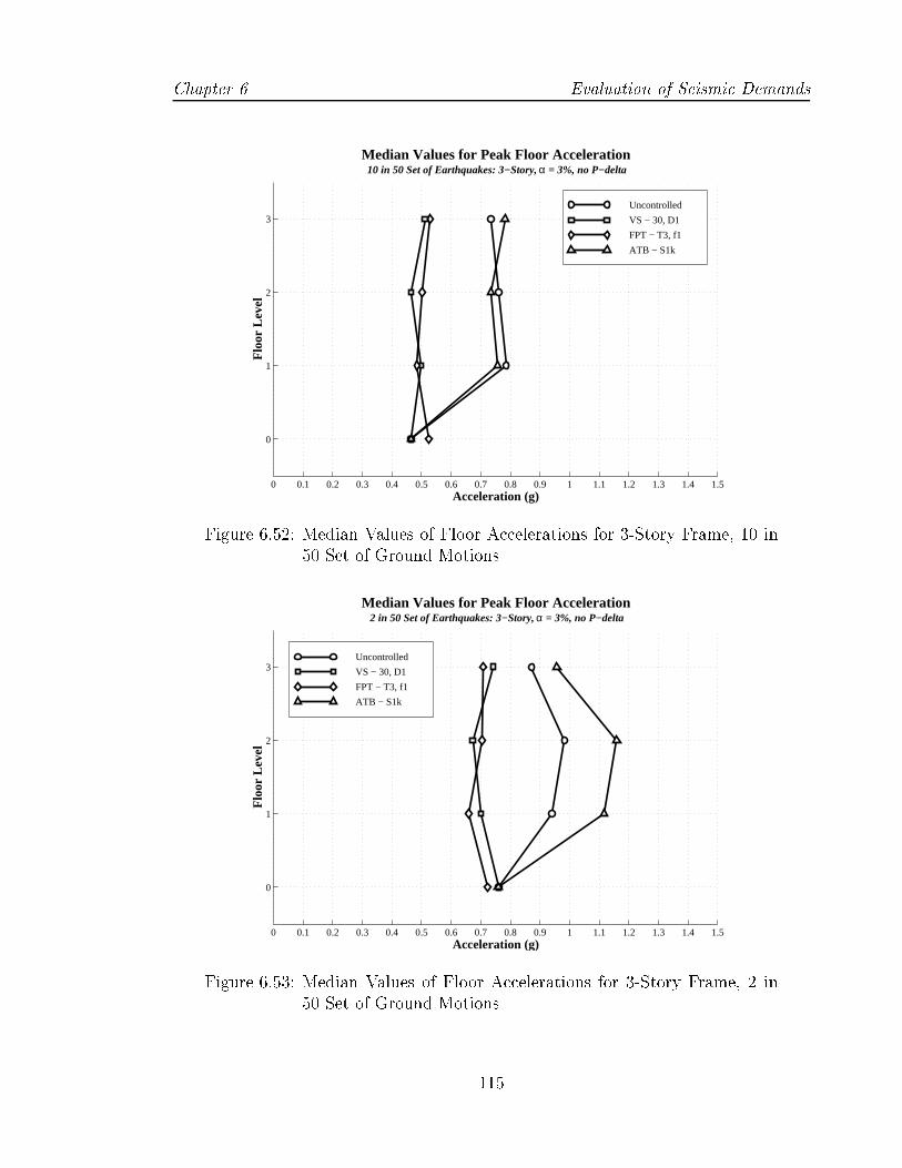
Chapter 6 Evaluation of Seismic Demands
0 0.1 0.2 0.3 0.4 0.5 0.6 0.7 0.8 0.9 1 1.1 1.2 1.3 1.4 1.5
0
1
2
3
Median Values for Peak Floor Acceleration 10 in 50 Set of Earthquakes: 3−Story, α = 3%, no P−delta
Acceleration (g)
Flo
or L
evel
Uncontrolled
VS − 30, D1
FPT − T3, f1
ATB − S1k
Figure 6.52: Median Values of Floor Accelerations for 3-Story Frame, 10 in50 Set of Ground Motions
0 0.1 0.2 0.3 0.4 0.5 0.6 0.7 0.8 0.9 1 1.1 1.2 1.3 1.4 1.5
0
1
2
3
Median Values for Peak Floor Acceleration 2 in 50 Set of Earthquakes: 3−Story, α = 3%, no P−delta
Acceleration (g)
Flo
or L
evel
Uncontrolled
VS − 30, D1
FPT − T3, f1
ATB − S1k
Figure 6.53: Median Values of Floor Accelerations for 3-Story Frame, 2 in50 Set of Ground Motions
115
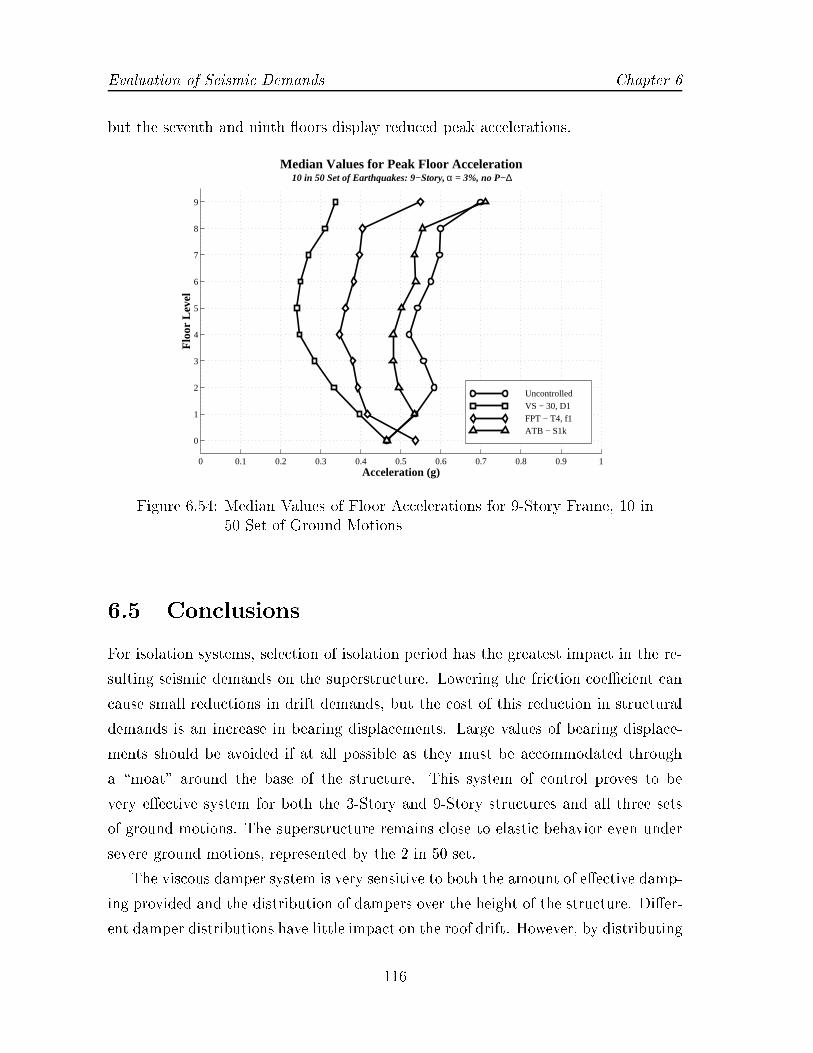
Evaluation of Seismic Demands Chapter 6
but the seventh and ninth oors display reduced peak accelerations.
0 0.1 0.2 0.3 0.4 0.5 0.6 0.7 0.8 0.9 1
0
1
2
3
4
5
6
7
8
9
Median Values for Peak Floor Acceleration 10 in 50 Set of Earthquakes: 9−Story, α = 3%, no P−∆
Acceleration (g)
Flo
or L
evel
UncontrolledVS − 30, D1 FPT − T4, f1ATB − S1k
Figure 6.54: Median Values of Floor Accelerations for 9-Story Frame, 10 in50 Set of Ground Motions
6.5 Conclusions
For isolation systems, selection of isolation period has the greatest impact in the re-
sulting seismic demands on the superstructure. Lowering the friction coeÆcient can
cause small reductions in drift demands, but the cost of this reduction in structural
demands is an increase in bearing displacements. Large values of bearing displace-
ments should be avoided if at all possible as they must be accommodated through
a \moat" around the base of the structure. This system of control proves to be
very e�ective system for both the 3-Story and 9-Story structures and all three sets
of ground motions. The superstructure remains close to elastic behavior even under
severe ground motions, represented by the 2 in 50 set.
The viscous damper system is very sensitive to both the amount of e�ective damp-
ing provided and the distribution of dampers over the height of the structure. Di�er-
ent damper distributions have little impact on the roof drift. However, by distributing
116

Chapter 6 Evaluation of Seismic Demands
0 0.1 0.2 0.3 0.4 0.5 0.6 0.7 0.8 0.9 1
0
1
2
3
4
5
6
7
8
9
Median Values for Peak Floor Acceleration 2 in 50 Set of Earthquakes: 9−Story, α = 3%, no P−∆
Acceleration (g)
Flo
or L
evel
UncontrolledVS − 30, D1 FPT − T4, f1ATB − S1k
Figure 6.55: Median Values of Floor Accelerations for 9-Story Frame, 2 in50 Set of Ground Motions
dampers according to relative story sti�ness and expected peak plastic deformations,
the drift demands are more evenly distributed among the di�erent stories. For the
same amount of e�ective damping, if the dampers are located in only a few stories the
system can by highly ine�ective. In the 9-Story structure, a system with dampers in
only three stories and 10% e�ective damping was designed. The resulting peak story
drift demands were higher than those of the uncontrolled structure in those stories
lacking dampers. In contrast, if smaller dampers are added at every story to produce
the same 10% e�ective damping, signi�cant reductions in drift result for all stories.
The capacity of the actuators for the ATB system contribute greatly to the ef-
fectiveness of the control system. Higher actuator capacities provide the controller
a greater opportunity to reduce drift demands. However, this same increased capac-
ity can result in systems which increase the demands from those of the uncontrolled
system.
Comparisons of the performance of three di�erent control strategies are presented
for all three sets of ground motions. The comparison is based on story drift, hys-
teretic energy, and oor acceleration demands. All three controllers were successful
117

Evaluation of Seismic Demands Chapter 6
in reducing the seismic demands, though no one system is consistently better than
the others at all three hazard levels.
For story drift demands, the values suggested for peak story drift angles in FEMA
273 are used as guidelines for judging structural performance. For short return peri-
ods, the addition of structural control reduced the median story drift by nearly 50%.
The most signi�cant impact of control occurs with the 2 in 50 ground motions. The
uncontrolled structure has a median response just under the collapse prevention limit.
Clear outliers are present in the data, with some response values exceeding 10% drift,
a response that is unsustainable by the physical system. The ATB and VS control
systems bring the median response to about 3%, with the VS system resulting in less
scatter in the data. The FPS isolation has the lowest median response, with values
of about 1.5%. Results for the 9-story structure follow a similar trend as those of the
3-story structure. Both the VS and FPS isolation are extremely e�ective at reducing
the peak story drift demands. The VS system proves to be most e�ective at higher
stories, while the FPS system is slightly less e�ective at the upper stories. For the
ATB control system, the actuators are placed on only the 1st, 2nd, and 8th stories.
The e�ect of this placement is that at high level excitations the drift demands at
stories without actuators are increased from the uncontrolled case. For comparison,
a VS system with dampers in only the same three stories and comparable peak forces
was designed. The resulting peak story drift demands were higher than those of
the uncontrolled structure in those stories lacking dampers. In contrast, if smaller
dampers are added at every story to produce the same amount of e�ective damping,
signi�cant reductions in drift result for all stories.
Residual drift values are used by FEMA 273 as an indicator of the inelastic damage
to the structural system. However, care must be taken in interpreting these values as
they can be misleading. In both the 50 in 50 set and 10 in 50 set of ground motions,
the median values for residual drifts of the control systems are close to negligible.
However, in the 2 in 50 set of ground motions, median values for all systems are
signi�cantly higher. The addition of the two passive controls decreases the median
drift demand value. However, the median value for the ATB system is greater than
that for the uncontrolled case, resulting in the appearance that the addition of this
control system appears to increase structural damage. However, closer analysis of the
response indicates that the ATB control keeps the structure from repeated inelastic
118
Chapter 6 Evaluation of Seismic Demands
deformations, as indicated by dissipated hysteretic energy results.
Normalized hysteretic energy (NHE) is used to provide information regarding the
cumulative damage to the structure. Normalization of the hysteretic energy values of
each element is performed by normalizing by the element's elastic energy capacity. In
the 50 in 50 set and 10 in 50 set, the addition of structural control reduces the amount
of energy that must be dissipated by the structural system to negligible values. The
only exception occurs with the active control for the 9-story structure under the 10
in 50 set, as its capacity is signi�cantly less than the two passive control strategies.
The ATB control consistently reduces the NHE demands at every story. In the 2 in
50 set, some dissipation of hysteretic energy occurs for all systems. The FPS system
proves to result in the least amount of energy demands for the structure, which agrees
with the results from the drift analyses.
Floor accelerations are of concern for damage to several nonstructural compo-
nents. Structural control systems have the bene�t of being capable of reducing both
acceleration and drift demands on the structure, which traditional methods such as
increasing building sti�ness cannot accomplish. The two passive control systems in-
vestigated are particularly e�ective at reducing oor accelerations as compared with
the uncontrolled structure. In the 3-story structure, the peak oor accelerations at
all oors were about that of the peak ground acceleration. In the 9-story structure,
accelerations at the middle oor levels were reduced below that of the ground. The
active control system had no signi�cant reduction in oor accelerations, as the system
was not speci�cally designed to control those responses. In the 2 in 50 set for the
3-story structure, oor accelerations were increased from the uncontrolled case with
the addition of the ATB controller.
119
Chapter 7
E�ects of Modeling on Seismic
Demands
7.1 Introduction
The seismic demands presented in Chapter 6 were based on several assumptions con-
cerning structural parameters and modeling. The response of any structure depends
on careful selection of those parameters so as to capture the signi�cant e�ects of
the structure. The focus of this chapter is to evaluate the e�ect of: 1) the level of
nonlinear modeling and analyses of the structure, 2) the initial sti�ness of the struc-
ture, and 3) the strain-hardening assumptions in force-deformation relationships of
the elements.
These investigations are performed using the 2 in 50 set of ground motions, for
which the e�ects of parameter variation is expected to be the greatest. The control
systems, as described in Section 6.4 are used in these studies. These systems are:
1. VS 30, D1: evenly distributed VS dampers with e�ective damping of 30%
2. FPS T3, f1: FPS isolation system with an isolation period of 3 seconds and a
sliding surface f1
3. FPS T4, f1: FPS isolation system with an isolation period of 4 seconds and a
sliding surface f1
4. ATB - S1k: ATB active system with actuator saturation of 1,000 kips
120

Chapter 7 E�ects of Modeling on Seismic Demands
The results are primarily analyzed considering global structural demands, specif-
ically the peak values of roof and story drift demands. Sensitivity investigations of
the e�ect of the initial period and strain-hardening ratio are performed only on the 3-
Story structure. The range of values chosen for those parameters endeavor to contain
the expected range in variation. Investigations into the e�ect of nonlinear analyses
also include investigations with the 9-Story structure, where the increased height of
the structure might impact secondary nonlinear e�ects, such as P-�.
7.2 E�ect of Nonlinearities on Controlled Struc-
tural Performance
One of the basic requirements for performance-based evaluation is con�dence in the
analyses results. A compromise between accuracy and eÆciency is usually necessary,
requiring a determination of the level of modeling and type of analysis required for this
purpose. An evaluation of the e�ect of nonlinear behavior on the demands resulting
from time history analyses is required. For this purpose, four di�erent evaluation
models containing di�erent levels of increasing nonlinearity were created for the 3-
story structure. They are:
� L - a centerline linear model with no second-order e�ect, such as P-�, being
considered.
� NL1 - �rst nonlinear model including only material yielding
� NL2 - builds upon NL1 and includes the e�ect of axial loads on the moment
capacity
� NL3 - same as NL2 with the e�ects of P-� introduced
Each control system as well as the original structure were then analyzed using the
above models using the 2 in 50 set of ground motions. A comparison of the rela-
tive demand reductions from each control strategy to the original structure is made
between the di�erent models. For a speci�c control system, the di�erences in drift
demands resulting from each evaluation model are compared.
121

E�ects of Modeling on Seismic Demands Chapter 7
7.2.1 3-Story Structure
The median values for peak story drifts of the uncontrolled structure are shown in
Figure 7.1. The results of model NL1 are essentially identical to those of model NL2,
indicating that the axial loads on the columns are not high enough to signi�cantly
a�ect the moment capacity of the columns. As a result, those values are not repeated
on the plot. A di�erence in the distribution of drift of the height can be seen in story
drift demands between the linear and nonlinear models NL2 and NL3. Though the
median value for drift demands are all below the level where any negative sti�ness
to lateral loads is observed, as indicated by the global pushover analysis shown in
Figure 6.1, P-� e�ects impact the demands of some of the extreme ground motions,
resulting in a increase in the median peak story drifts. The scatter in the peak
0 0.005 0.01 0.015 0.02 0.025 0.03 0.035 0.04 0.045 0.050
1
2
3
Median Values for Peak Story Drift Angles for Uncontrolled System 2 in 50 Set of Earthquakes: 3−Story, α = 3%, no P−∆
Flo
or L
evel
Drift Angle
L Model
NL2 Model
NL3 Model
Figure 7.1: E�ect of Modeling on Median Values for Peak Story Drift De-mands, 2 in 50 Set of Ground Motions
roof drift demands of each system for these models can be observed in Figures 7.2
through 7.4, with the median indicated by a solid horizontal line. The presence of
outliers occurs in all models, especially for the uncontrolled structure. The linear
model, L, displays a fairly even scatter of the response about the median values. The
122

Chapter 7 E�ects of Modeling on Seismic Demands
FPS isolation system displays the least scatter, with only 3 records having higher
demands than the tight clustering about the median. The demands from the NL2
evaluation model have slightly less scatter for most records. However, the severe
outlier values are still present. For the isolation system, the response of the outlier
points is signi�cantly higher. The consideration of P-� e�ects with the NL3 model
only has a signi�cant impact on the uncontrolled response, with more outlier points
than were present in the NL2 model
Uncontrolled VS − 30, D1 FPS − T3, f1 ATB − S1k0
0.01
0.02
0.03
0.04
0.05
0.06
0.07
0.08
Drif
t Ang
le
Maximum Roof Drift Angles for L Model 2 in 50 Set of Earthquakes: 3−Story Structure
Figure 7.2: Maximum Roof Drift Demands for 3-Story Frame L Model, 2 in50 Set of Ground Motions
The amount of peak roof drift reduction for each control system from the original
structure, based on each type of nonlinear model, is shown on Table 7.1. For this
structure, little di�erence exists between estimated roof drift reductions among the
di�erent nonlinear models. However, linear models can severely overestimate the
e�ectiveness of the systems when comparing controlled performance with uncontrolled
response. Note that the impact of P-� is apparent in the percent reduction factors
in the 2 in 50 set, especially for the VS and ATB control systems, whose demands
are only minutely impacted by P-� e�ects.
Di�erences are also apparent in the distribution of peak story drift demands over
123

E�ects of Modeling on Seismic Demands Chapter 7
Uncontrolled VS − 30, D1 FPS − T3, f1 ATB − S1k0
0.01
0.02
0.03
0.04
0.05
0.06
0.07
0.08
Drif
t Ang
le
Maximum Roof Drift Angles for NL2 Model 2 in 50 Set of Earthquakes: 3−Story, α = 3%, no P−∆
Figure 7.3: Maximum Roof Drift Demands for 3-Story Frame NL2 Model, 2in 50 Set of Ground Motions
Uncontrolled VS − 30, D1 FPS − T3, f1 ATB − S1k0
0.01
0.02
0.03
0.04
0.05
0.06
0.07
0.08
Drif
t Ang
le
Maximum Roof Drift Angles for NL3 Model 2 in 50 Set of Earthquakes: 3−Story, α = 3%, P−∆
Figure 7.4: Maximum Roof Drift Demands for 3-Story Frame NL3 Model, 2in 50 Set of Ground Motions
124
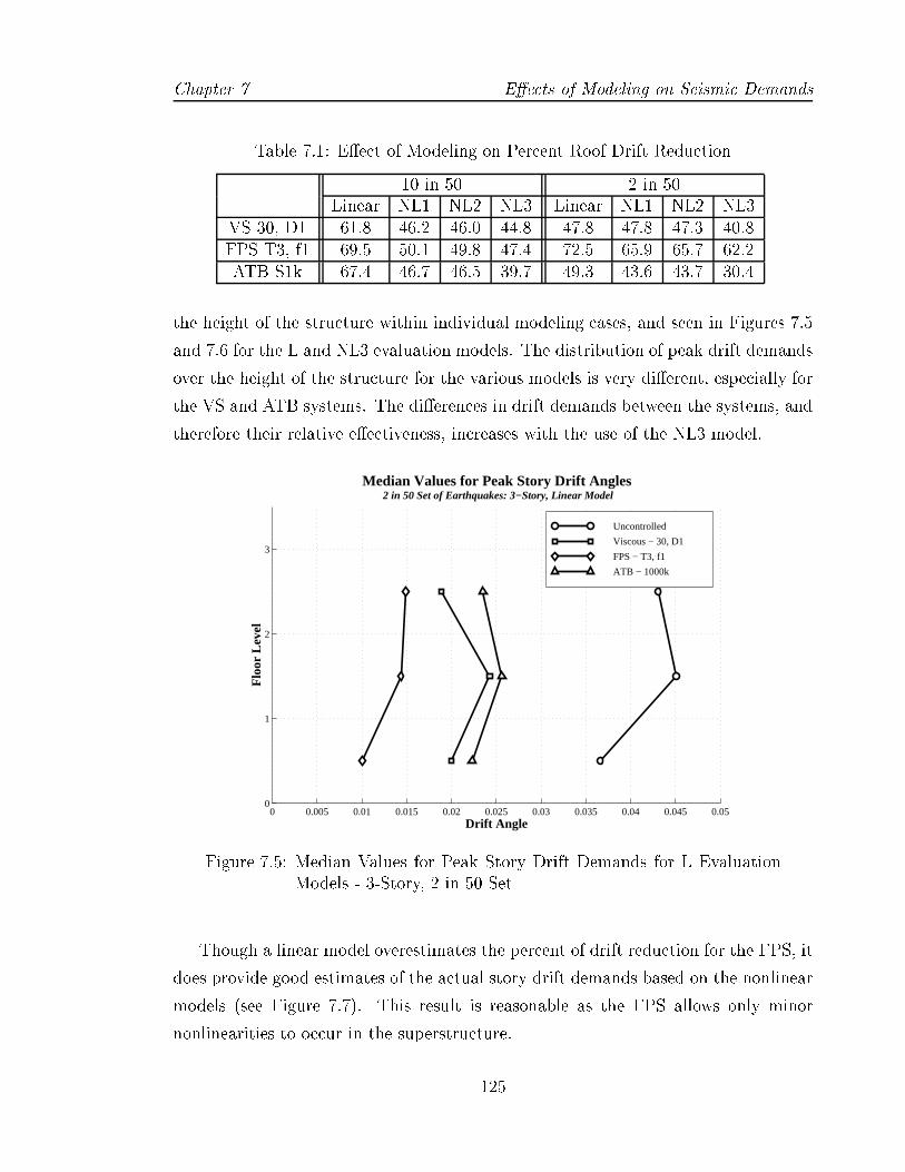
Chapter 7 E�ects of Modeling on Seismic Demands
Table 7.1: E�ect of Modeling on Percent Roof Drift Reduction
10 in 50 2 in 50Linear NL1 NL2 NL3 Linear NL1 NL2 NL3
VS 30, D1 61.8 46.2 46.0 44.8 47.8 47.8 47.3 40.8FPS T3, f1 69.5 50.1 49.8 47.4 72.5 65.9 65.7 62.2ATB S1k 67.4 46.7 46.5 39.7 49.3 43.6 43.7 30.4
the height of the structure within individual modeling cases, and seen in Figures 7.5
and 7.6 for the L and NL3 evaluation models. The distribution of peak drift demands
over the height of the structure for the various models is very di�erent, especially for
the VS and ATB systems. The di�erences in drift demands between the systems, and
therefore their relative e�ectiveness, increases with the use of the NL3 model.
0 0.005 0.01 0.015 0.02 0.025 0.03 0.035 0.04 0.045 0.050
1
2
3
Median Values for Peak Story Drift Angles 2 in 50 Set of Earthquakes: 3−Story, Linear Model
Drift Angle
Flo
or L
evel
Uncontrolled
Viscous − 30, D1
FPS − T3, f1
ATB − 1000k
Figure 7.5: Median Values for Peak Story Drift Demands for L EvaluationModels - 3-Story, 2 in 50 Set
Though a linear model overestimates the percent of drift reduction for the FPS, it
does provide good estimates of the actual story drift demands based on the nonlinear
models (see Figure 7.7). This result is reasonable as the FPS allows only minor
nonlinearities to occur in the superstructure.
125

E�ects of Modeling on Seismic Demands Chapter 7
0 0.005 0.01 0.015 0.02 0.025 0.03 0.035 0.04 0.045 0.050
1
2
3
Median Values for Peak Story Drift Angles 2 in 50 Set of Earthquakes: 3−Story, α = 3%, P−∆
Drift Angle
Flo
or L
evel
Uncontrolled
Viscous − 30, D1
FPS − T3, f1
ATB − 1000k
Figure 7.6: Median Values for Peak Story Drift Demands for NL3 EvaluationModels - 3-Story, 2 in 50 Set
0 0.005 0.01 0.015 0.02 0.025 0.03 0.035 0.04 0.045 0.050
1
2
3
Median Values for Peak Story Drift Angles for T3, f1 System 2 in 50 Set of Earthquakes: 3−Story, α = 3%, no P−∆
Flo
or L
evel
Drift Angle
L Model
NL2 Model
NL3 Model
Figure 7.7: E�ect of Modeling on Median Values for Peak Story Drift De-mands for FPS T3 - f1, 2 in 50 Set
126
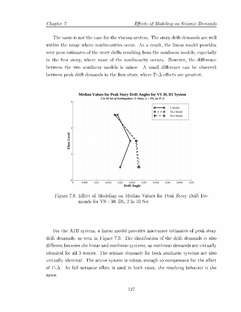
Chapter 7 E�ects of Modeling on Seismic Demands
The same is not the case for the viscous system. The story drift demands are well
within the range where nonlinearities occur. As a result, the linear model provides
very poor estimates of the story drifts resulting from the nonlinear models, especially
in the �rst story, where most of the nonlinearity occurs. However, the di�erence
between the two nonlinear models is minor. A small di�erence can be observed
between peak drift demands in the �rst story, where P-� e�ects are greatest.
0 0.005 0.01 0.015 0.02 0.025 0.03 0.035 0.04 0.045 0.050
1
2
3
Median Values for Peak Story Drift Angles for VS 30, D1 System 2 in 50 Set of Earthquakes: 3−Story, α = 3%, no P−∆
Flo
or L
evel
Drift Angle
L Model
NL2 Model
NL3 Model
Figure 7.8: E�ect of Modeling on Median Values for Peak Story Drift De-mands for VS - 30, D1, 2 in 50 Set
For the ATB system, a linear model provides inaccurate estimates of peak story
drift demands, as seen in Figure 7.9. The distribution of the drift demands is also
di�erent between the linear and nonlinear systems, as nonlinear demands are virtually
identical for all 3 stories. The seismic demands for both nonlinear systems are also
virtually identical. The active system is robust enough to compensate for the e�ect
of P-�. As full actuator e�ort is used in both cases, the resulting behavior is the
same.
127

E�ects of Modeling on Seismic Demands Chapter 7
0 0.005 0.01 0.015 0.02 0.025 0.03 0.035 0.04 0.045 0.050
1
2
3
Median Values for Peak Story Drift Angles for T3, f1 System 2 in 50 Set of Earthquakes: 3−Story, α = 3%, no P−∆
Flo
or L
evel
Drift Angle
L Model
NL2 Model
NL3 Model
Figure 7.9: E�ect of Modeling on Median Values for Peak Story Drift De-mands for ATB - S1k, 2 in 50 Set
7.2.2 9-Story Structure
Similar trends are observed with the 9-Story structure as discussed in the previous
section. A linear model analysis results in signi�cantly higher story drift demands to
those of the nonlinear analyses as seen in Figure 7.10. Also, the distribution of drift
demands over the stories for the linear model does not re ect the increased story drift
demands in the lower stories. Again, little is gained through the consideration of P-�
e�ects even with this taller structure. The drift demands are all below the level where
any negative sti�ness to lateral loads is observed, as indicated by the stable plateau
in the global pushover analysis shown in Figure 6.1
As the FPS system maintains the superstructure close to its elastic limit, a linear
dynamic analysis does provide good estimates of the actual drift demands as com-
pared to those from the nonlinear models, as shown in Figure 7.11. Only very minor
di�erences can be observed by including the e�ects of P-� in the analyses.
Though the story drift demands for the structure with VS dampers, principally
for the lower 6 stories, are well within the range where nonlinearities occur, The linear
model provides reasonable estimates of the story drifts resulting from the nonlinear
128

Chapter 7 E�ects of Modeling on Seismic Demands
0 0.01 0.02 0.03 0.04 0.05 0.060
1
2
3
4
5
6
7
8
9
Median Values for Peak Story Drift Angles for Uncontrolled System 2 in 50 Set of Earthquakes: 9−Story, α = 3%, no P−∆
Drift Angle
Flo
or L
evel
NL2
Linear
NL3
Figure 7.10: E�ect of Modeling on Median Values for Peak Story Drift De-mands for 9-Story Structure, 2 in 50 Set
0 0.005 0.01 0.015 0.02 0.025 0.03 0.035 0.04 0.045 0.050
1
2
3
4
5
6
7
8
9
Median Values for Peak Story Drift Angles for System FPS T4 − f1 2 in 50 Set of Earthquakes: 9−Story, α = 3%, no P−∆
Drift Angle
Flo
or L
evel
NL2
Linear
NL3
Figure 7.11: E�ect of Modeling on Median Values for Peak Story Drift De-mands for 9-Story Structure with FPS T4 - f1, 2 in 50 Set
129
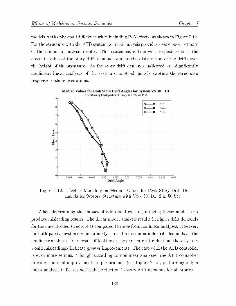
E�ects of Modeling on Seismic Demands Chapter 7
models, with only small di�erence when including P-� e�ects, as shown in Figure 7.12.
For the structure with the ATB system, a linear analysis provides a very poor estimate
of the nonlinear analysis results. This statement is true with respect to both the
absolute value of the story drift demands and to the distribution of the drifts over
the height of the structure. As the story drift demands indicated are signi�cantly
nonlinear, linear analyses of the system cannot adequately capture the structures
response to these excitations.
0 0.005 0.01 0.015 0.02 0.025 0.03 0.035 0.04 0.045 0.050
1
2
3
4
5
6
7
8
9
Median Values for Peak Story Drift Angles for System VS 30 − D1 2 in 50 Set of Earthquakes: 9−Story, α = 3%, no P−∆
Drift Angle
Flo
or L
evel
NL2
Linear
NL3
Figure 7.12: E�ect of Modeling on Median Values for Peak Story Drift De-mands for 9-Story Structure with VS - 30, D1, 2 in 50 Set
When determining the impact of additional control, utilizing linear models can
produce misleading results. The linear model analysis results in higher drift demands
for the uncontrolled structure as compared to those from nonlinear analyses. However,
for both passive systems a linear analysis results in comparable drift demands as the
nonlinear analyses. As a result, if looking at the percent drift reduction, those system
would misleadingly indicate greater improvements. The case with the ATB controller
is even more serious. Though according to nonlinear analyses, the ATB controller
provides minimal improvements in performance (see Figure 7.15), performing only a
linear analysis indicates noticeable reduction in story drift demands for all stories.
130
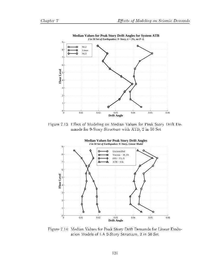
Chapter 7 E�ects of Modeling on Seismic Demands
0 0.01 0.02 0.03 0.04 0.05 0.060
1
2
3
4
5
6
7
8
9
Median Values for Peak Story Drift Angles for System ATB 2 in 50 Set of Earthquakes: 9−Story, α = 3%, no P−∆
Drift Angle
Flo
or L
evel
NL2
Linear
NL3
Figure 7.13: E�ect of Modeling on Median Values for Peak Story Drift De-mands for 9-Story Structure with ATB, 2 in 50 Set
0 0.01 0.02 0.03 0.04 0.05 0.060
1
2
3
4
5
6
7
8
9
Median Values for Peak Story Drift Angles 2 in 50 Set of Earthquakes: 9−Story, Linear Model
Drift Angle
Flo
or L
evel
Uncontrolled
Viscous − 30, D1
FPS − T3, f1
ATB − S1k
Figure 7.14: Median Values for Peak Story Drift Demands for Linear Evalu-ation Models of LA 9-Story Structure, 2 in 50 Set
131

E�ects of Modeling on Seismic Demands Chapter 7
0 0.005 0.01 0.015 0.02 0.025 0.03 0.035 0.04 0.045 0.050
1
2
3
4
5
6
7
8
9
Median Values for Peak Story Drift Angles 2 in 50 Set of Earthquakes: 9−Story, α = 3%, P−∆
Drift Angle
Flo
or L
evel
Uncontrolled
Viscous − 30, D1
FPS − T4, f1
Figure 7.15: Median Values for Peak Story Drift Demands for Linear Evalu-ation Models of LA 9-Story Structure, 2 in 50 Set
7.3 E�ect of Initial Sti�ness on Dynamic Response
The response of the structure is a�ected by the presence of cladding, partition walls,
and other nonstructural elements. These elements are expected to increase the elastic
sti�ness of the structure, though the exact amount is unknown. On the other hand,
moment-resisting connections may have some additional exibility associated with
them that is not originally considered. Furthermore, uncertainty in material prop-
erties may result in a more exible structure. To assess the range of e�ect changes
in sti�ness may have on the seismic response, the elastic sti�ness of all columns and
beams is reduced by constant amounts. The change is equivalent to reducing the �rst
mode period by factors of 0.5, 0.75, 1.25, and 2.00.
The median story drift demands for the uncontrolled 3-story structure under the 2
in 50 set of ground motions are shown in Figure 7.16. The changes in sti�ness a�ects
the drift demands in the upper stories more than in the �rst story. In general, the
impact of initial period variation can be estimated from the spectrum plots.
The median story drift demands for the 3-story structure with a FPS system
designed with an isolation period of 3 seconds under the 2 in 50 set of ground motions
132
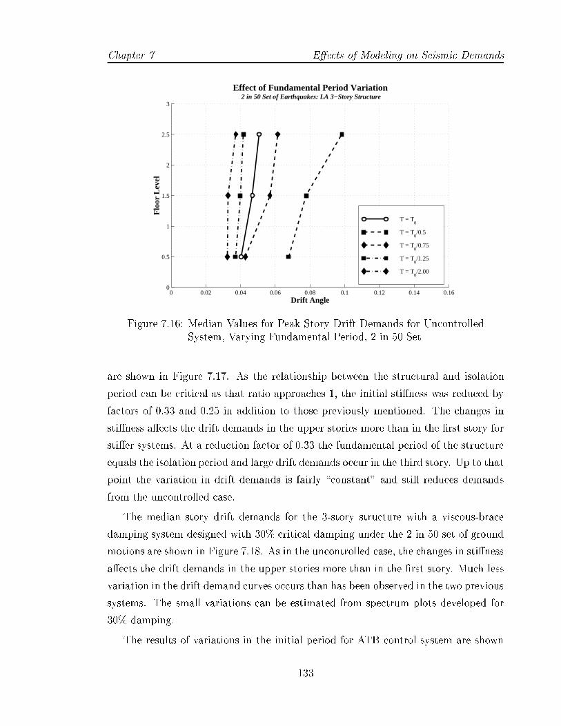
Chapter 7 E�ects of Modeling on Seismic Demands
0 0.02 0.04 0.06 0.08 0.1 0.12 0.14 0.160
0.5
1
1.5
2
2.5
3
Drift Angle
Flo
or L
evel
Effect of Fundamental Period Variation 2 in 50 Set of Earthquakes: LA 3−Story Structure
T = T0
T = T0/0.5
T = T0/0.75
T = T0/1.25
T = T0/2.00
Figure 7.16: Median Values for Peak Story Drift Demands for UncontrolledSystem, Varying Fundamental Period, 2 in 50 Set
are shown in Figure 7.17. As the relationship between the structural and isolation
period can be critical as that ratio approaches 1, the initial sti�ness was reduced by
factors of 0.33 and 0.25 in addition to those previously mentioned. The changes in
sti�ness a�ects the drift demands in the upper stories more than in the �rst story for
sti�er systems. At a reduction factor of 0.33 the fundamental period of the structure
equals the isolation period and large drift demands occur in the third story. Up to that
point the variation in drift demands is fairly \constant" and still reduces demands
from the uncontrolled case.
The median story drift demands for the 3-story structure with a viscous-brace
damping system designed with 30% critical damping under the 2 in 50 set of ground
motions are shown in Figure 7.18. As in the uncontrolled case, the changes in sti�ness
a�ects the drift demands in the upper stories more than in the �rst story. Much less
variation in the drift demand curves occurs than has been observed in the two previous
systems. The small variations can be estimated from spectrum plots developed for
30% damping.
The results of variations in the initial period for ATB control system are shown
133

E�ects of Modeling on Seismic Demands Chapter 7
0 0.02 0.04 0.06 0.08 0.1 0.12 0.14 0.160
1
2
3
Drift Angle
Flo
or L
evel
Effect of Fundamental Period Variation on System with FPS 2 in 50 Set of Earthquakes: LA 3−Story Structure
T = To
T = To/0.25
T = To/0.33
T = To/0.5
T = To/0.625
T = To/0.75
T = To/1.25
T = To/2.00
Figure 7.17: Median Values for Peak Story Drift Demands for FPS IsolationSystem T3, Varying Fundamental Period, 2 in 50 Set
0 0.02 0.04 0.06 0.08 0.1 0.12 0.14 0.160
1
2
3
Drift Angle
Flo
or L
evel
Effect of Fundamental Period Variation on System with Viscous Dampers 2 in 50 Set of Earthquakes: LA 3−Story Structure
T = To
T = To/0.5
T = To/0.625
T = To/0.75
T = To/1.25
T = To/2.00
Figure 7.18: Median Values for Peak Story Drift Demands for VS 30 System,Varying Fundamental Period, 2 in 50 Set
134
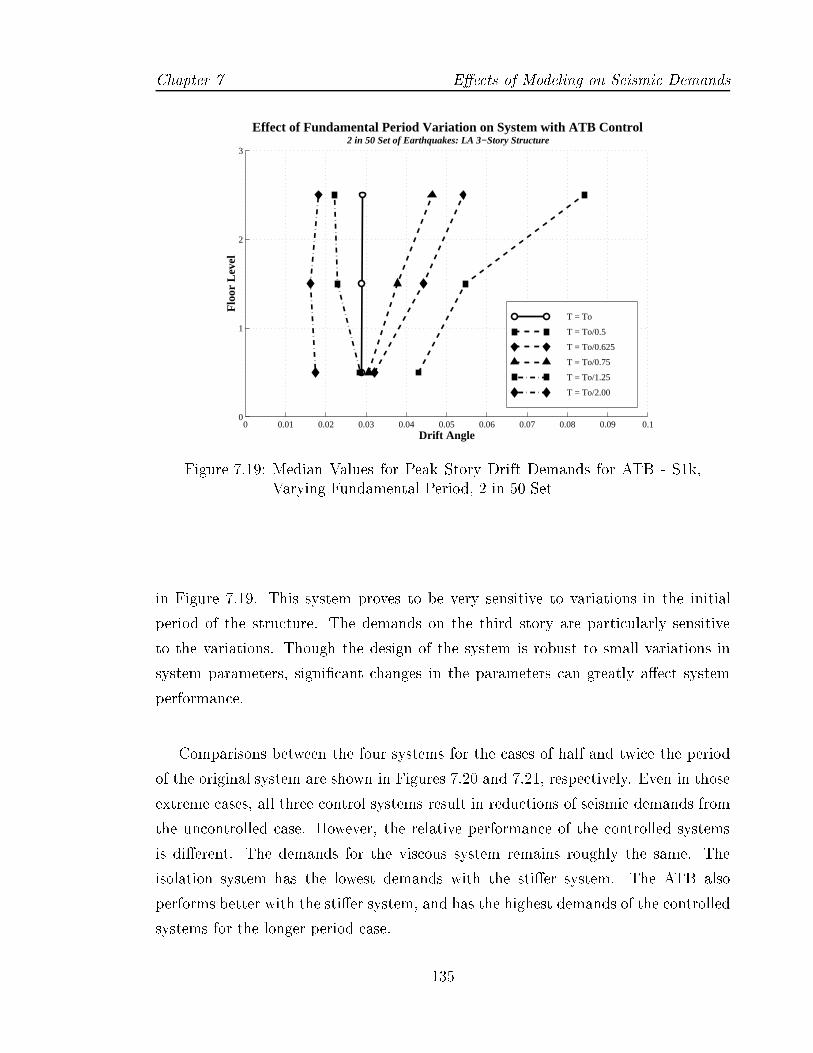
Chapter 7 E�ects of Modeling on Seismic Demands
0 0.01 0.02 0.03 0.04 0.05 0.06 0.07 0.08 0.09 0.10
1
2
3
Drift Angle
Flo
or L
evel
Effect of Fundamental Period Variation on System with ATB Control 2 in 50 Set of Earthquakes: LA 3−Story Structure
T = To
T = To/0.5
T = To/0.625
T = To/0.75
T = To/1.25
T = To/2.00
Figure 7.19: Median Values for Peak Story Drift Demands for ATB - S1k,Varying Fundamental Period, 2 in 50 Set
in Figure 7.19. This system proves to be very sensitive to variations in the initial
period of the structure. The demands on the third story are particularly sensitive
to the variations. Though the design of the system is robust to small variations in
system parameters, signi�cant changes in the parameters can greatly a�ect system
performance.
Comparisons between the four systems for the cases of half and twice the period
of the original system are shown in Figures 7.20 and 7.21, respectively. Even in those
extreme cases, all three control systems result in reductions of seismic demands from
the uncontrolled case. However, the relative performance of the controlled systems
is di�erent. The demands for the viscous system remains roughly the same. The
isolation system has the lowest demands with the sti�er system. The ATB also
performs better with the sti�er system, and has the highest demands of the controlled
systems for the longer period case.
135

E�ects of Modeling on Seismic Demands Chapter 7
0 0.01 0.02 0.03 0.04 0.050
1
2
3
Drift Angle
Flo
or L
evel
Comparison of Median Values of Peak Story Drift Demands: T = To/2 2 in 50 Set of Earthquakes: 3−Story Structure
Uncontrolled
Viscous Dampers
FPS Isolation
ATB
Figure 7.20: Median Values for Peak Story Drift Demands for Half the Orig-inal Fundamental Period, 2 in 50 Set
0 0.01 0.02 0.03 0.04 0.05 0.06 0.07 0.08 0.09 0.1 0.11 0.120
1
2
3
Drift Angle
Flo
or L
evel
Comparison of Median Values of Peak Story Drift Demands: T = To/0.5 2 in 50 Set of Earthquakes: 3−Story Structure
Uncontrolled
Viscous Dampers
FPS Isolation
ATB
Figure 7.21: Median Values for Peak Story Drift Demands for Twice theOriginal Fundamental Period, 2 in 50 Set
136
Chapter 7 E�ects of Modeling on Seismic Demands
7.4 E�ect of Variations in Strain-Hardening Ratio
The modeling of the post-yield sti�ness of frame element involve two major assump-
tions. The �rst assumption concerns the use of a stable force-deformation relationship,
which may not account for strength deterioration or sti�ness degradation. The second
assumption is in the determination of the value assigned to the post-yield sti�ness
of the element, �, which in this study is given as a fraction of the elastic sti�ness
of the frame member. This section investigates the e�ect of the second assumption
on the resulting drift demands of the structure. The 3-Story structure is analyzed
using the basic nonlinear model utilized in Chapter 6, NL2, under the 2 in 50 set of
ground motions. The values of the strain-hardening ratio of all frame members are
kept the same and taken to be either 0%, 3%, 5%, or 10%. These values are expected
to contain the expected range of possible strain-hardening for steel frame members.
The impact of varying the strain-hardening ratio is minor for the original un-
controlled structure, as seen in Figure 7.22. The trend in increasing the post-yield
sti�ness follows expectations, with increasing sti�ness resulting in a decrease in the
peak story drift demands.
The impact on strain-hardening variation is very minor with the FPS isolation
system, as seen in Figure 7.23. As the structure remains very close to the elastic limit,
the impact of changing post-yield behavior is small. However, in the VS system which
undergoes signi�cantly greater inelasticity, changing strain-hardening ratios has an
even smaller impact, shown in Figure 7.24. The ATB system proves to be the most
sensitive of the three control systems to variations in the strain-hardening ratio, as
shown in Figure 7.25. The impact is still small, however, and noticeably less than the
impact on the uncontrolled structure.
7.5 Conclusions
The use of linear evaluation models generally result in inaccurate estimation of the
seismic demands for the di�erent systems analyzed, both in terms of relative and
absoluted demand values. The relative impact of the addition of the di�erent control
systems depends on how far the sesimic demands drive the structure into the nonlinear
range. The use of a linear evaluation model for the FPS isolation system represents
137

E�ects of Modeling on Seismic Demands Chapter 7
0 0.01 0.02 0.03 0.04 0.05
1
2
3
Drift Angle
Flo
or L
evel
Effect of Variation in Percent Strain Hardening 2 in 50 Set of Earthquakes: LA 3−Story Structure
α = 0% α = 3% α = 5% α = 10%
Figure 7.22: Median Values for Peak Story Drift Demands for UncontrolledSystem, Variation Strain-Hardening Ratio, 2 in 50 Set
0 0.01 0.02 0.03 0.04 0.05
1
2
3
Drift Angle
Flo
or L
evel
Effect of Variation in Percent Strain Hardening on System with FPS 2 in 50 Set of Earthquakes: LA 3−Story Structure
α = 0% α = 3% α = 5% α = 10%
Figure 7.23: Median Values for Peak Story Drift Demands for FPS T3 Sys-tem T3, Variation Strain-Hardening Ratio, 2 in 50 Set
138

Chapter 7 E�ects of Modeling on Seismic Demands
0 0.01 0.02 0.03 0.04 0.05
1
2
3
Drift Angle
Flo
or L
evel
Effect of Variation in Percent Strain Hardening on System with ATB 2 in 50 Set of Earthquakes: LA 3−Story Structure
α = 0% α = 3% α = 5% α = 10%
Figure 7.24: Median Values for Peak Story Drift Demands for VS 30 System,Variation Strain-Hardening Ratio, 2 in 50 Set
0 0.01 0.02 0.03 0.04 0.05
1
2
3
Drift Angle
Flo
or L
evel
Effect of Variation in Percent Strain Hardening on System with ATB 2 in 50 Set of Earthquakes: LA 3−Story Structure
α = 0% α = 3% α = 5% α = 10%
Figure 7.25: Median Values for Peak Story Drift Demands for ATB System,Variation Strain-Hardening Ratio, 2 in 50 Set
139
E�ects of Modeling on Seismic Demands Chapter 7
the only case where a reasonable estimate of the seismic demands is achieved. This
behavior occurs as the isolation system maintains the behavior of the superstructure
close to its elastic range. However, even in the isolated system, the linear evaluation
models underestimate the amount of scatter in the results. Furthermore, though the
superstructure can be modeled elastically, the behavior of the bearing is inherently
nonlinear, so a nonlinear time history analysis of the system needs to be performed.
Nonlinear evaluation models are required for the other systems in order to achieve
reasonable demand estimates. The distribution of drifts over the height of the struc-
ture are particularly a�ected by the choice of linear vs. nonlinear analyses. In the
ATB controlled system, the seismic demands resulting from a linear analysis indicate
that peak drift demands are reduced in all stories of the structure. Drift demands
resulting from a nonlinear analysis, however, indicate that peak drift demands in sto-
ries without actuators are actually increased from the uncontrolled response. In the
structures considered, the consideration of P-� e�ects in the calculation of demands
has little e�ect on the results, especially for the control systems. As these systems
reduce the demands on the structure, the chance of a system entering the negative-
sti�ness response range is reduced. This assumption should be checked with systems
where P-� e�ects are more pronounced.
A sensitivity analysis of these control strategies to the initial period and strain-
hardening ratio was also presented. As these systems reduce drift demands, the
excursion into the inelastic range is reduced. As a result, sensitivity to the strain-
hardening ration is minor. The systems are more sensitive to variations in the initial
period of the structure. The isolation and ATB systems are particularly sensitive
to increases in period. In contrast, the viscous damper system is fairly insensitive
to variations in initial period. In all cases, however, the addition of control reduced
seismic demands from the uncontrolled structure.
140

Chapter 8
Probabilistic Seismic Control
Analysis
8.1 Introduction
Current performance-based codes provide guidelines for calculation of seismic demand
for a scenario event; the resulting seismic demand is then compared with the allowable
limit given, such as those provided in Section 2.5. This procedure generally accounts
for the uncertainty present in ground motion excitation; however, the uncertainty
and variability in the demand estimation generally is not considered. One approach
to addressing this issue is the development of probabilistic seismic demand curves,
so that the probability that any damage measure exceeds a pre-determined allowable
limit can be determined.
Procedures for developing probabilistic seismic demand curves can be found in
literature (Cornell 1996; Wen 1995). These methodologies generally relate a record-
speci�c quantity, typically the linear elastic spectral acceleration at a characteristic
building frequency, to a structural response parameter, such as interstory drift, so as
to estimate the probability of exceeding the selected structural response parameter.
Di�erences between methods arise, at least in part, due to di�ering objectives by the
researchers. A comparison between the methods proposed by Cornell and Wen and
the current guidelines in FEMA 273 was performed by Shome, Cornell, Bazzurro, and
Carballo (1997).
In this study, the procedure proposed by Cornell, and explicitly described in Luco
141

Probabilistic Seismic Control Analysis Chapter 8
and Cornell (1998) with respect to its application in the SAC project, is used to
assess the annual exceedance probabilities for interstory drift demands. This chapter
summarizes this procedure and utilizes it to generate interstory drift hazard curves
for the di�erent control strategies previously discussed in Chapter 6.
8.2 Background
The �nal objective of the methodology devised by Cornell is the estimation of the
annual probability of exceedance of a given level of inelastic response in a speci�c
MDOF structure. The structure is located at a speci�c site with an associated poten-
tial seismic hazard. The response of interest can be any structural response param-
eter, representing either local or global structural demands. The procedure couples
conventional Probabilistic Seismic Hazard Analysis (PSHA) with nonlinear dynamic
structural analyses in order to determine the annual probability of exceedance of a
given response parameter. This procedure is referred to as the Probabilistic Seis-
mic Demand Analysis (PSDA). These concepts are then extended to the analysis of
controlled response, referred to as Probabilistic Seismic Control Analysis (PSCA).
8.2.1 Probabilistic Seismic Hazard Analysis (PSHA)
In view of the rareness of seismic events and the variability of their characteristics, the
description of the seismic threat in probabilistic terms has become common practice.
The earliest work in this area has de�ned this threat in terms of some measure of
the ground motion intensity, such as peak ground acceleration (PGA). More recent
work has commonly sought to characterize the ground motion by its response spectral
acceleration Sa|i.e., the peak acceleration the earthquake will induce in a 1-DOF
system with a speci�ed period T and damping ratio �. Commonly, T and � are chosen
to describe the properties of the �rst mode of the building of interest. Alternatively,
one may instead consider the peak spectral velocity Sv or displacement Sd. In any
case, the aim is to describe the probability that the ground motion characteristic of
interest (PGA, Sa, Sv, or Sd) is exceeded over a reference period of interest.
For example, an existing site hazard curve for spectral acceleration provides the
probability of exceeding any particular spectral acceleration, Sa(T; �), for a given
142

Chapter 8 Probabilistic Seismic Control Analysis
period, T , and damping ratio, �. The elastic spectral acceleration at the fundamental
period of the model structure is typically used since it is usually an e�ective structure-
speci�c measure of ground motion intensity for predicting the nonlinear response of
buildings (Shome et al. 1997). Research has also been conducted that evaluates the
e�ect of performing the analysis using a mixture or vectorized Sa values (Shome and
Cornell 1998). An \e�ective" intensity measure for earthquake records is one for
which the record-to-record dispersion of the drift response given the intensity level is
relatively small, and for which a hazard analysis is available. The particular choice
of ground motion intensity measure, as indicated previously, is not critical to the
procedure.
The probability that Sa exceeds a critical value scr in an arbitrary earthquake is
formally written as follows:
P [Sa > scr] = GSa(scr) =
ZZm;r
P [Sa > scr jM = m;R = r] fM;R(m; r) dmdr (8.1)
in which fM;R(m; r) is the joint probability density function that describes the mag-
nitude M and site-to-source distance R of an arbitrary event. Equation (8.1) is com-
monly evaluated numerically, and has become known as Probabilistic Seismic Hazard
Analysis (Cornell 1968) or \PSHA". Final results are generally rescaled by a rate � of
all events being modeled, leading to a mean hazard rate H(s) associated with those
seismic events that produce Sa > scr:
HSa(scr) = �GSa(scr) = �
ZZm;r
P [Sa > scrjM = m;R = r] fM;R(m; r) dmdr (8.2)
The quantity HSa, expressed as a function of scr, is the typical output of a PSHA
computation. As a simple parametric representation, Cornell (1996) has suggested
that the net result is often well-approximated by a power-law relation of the form:
H(Sa) = k0S�k1a (8.3)
where H(Sa) is the annual probability of exceeding a given Sa, and k0 and k1 are
constants obtained by �tting the function to results from a PSHA near the return
period of interest. The coeÆcients k0 and k1 thus serve to characterize the seismic
143

Probabilistic Seismic Control Analysis Chapter 8
threat at a given site of interest. The above approximation has the advantage of being
linear in log-log space and has been shown to be satisfactory over a range of spectral
accelerations (Shome 1999).
8.2.2 Probabilistic Seismic Demand Analysis (PSDA)
Unfortunately, Sa does not provide suÆcient information to determine the precise
response of actual buildings, which generally show both nonlinear and multi-degree-
of-freedom (MDOF) behavior. Indeed, a growing trend toward \performance-based"
seismic design exists, in which a range of increasingly rare hazards are speci�ed, to-
gether with a correspondingly increasing level of permissible \damage" (i.e., nonlinear
behavior). These requirements imply the need for explicit recognition, and the statis-
tical quanti�cation, of the degree of nonlinear behavior|e.g., the drift demand Æ|as
a function of the desired exceedance rate, such as the return period.
Extension of conventional PSHA, to directly describe the seismic demand Æ of
a complex, nonlinear structure, has become known as probabilistic seismic demand
analysis (\PSDA"). In general, the calculation of the probability of exceedance of
a level y of any damage parameter Y involves the summation of the probability
of exceeding a level y for the parameter Y over all possible seismic sources. For
a given seismic source, the determination of the probability of exceeding a level y
for the parameter Y must consider 1) the probability of exceeding a level y for a
given spectral acceleration, earthquake magnitude, and distance to source, 2) the
probability distribution of the spectral acceleration given a magnitude and distance,
and 3) the probability distribution of magnitude and distance for the source. This
relationship can be expressed mathematically as follows:
P (Y > y) =NXi=1
�i
ZZZP [Y > y j sa; m; r]i � fSajM;R(sa j m; r)i
� fM;R(m; r)i dsa dm dr
(8.4)
where N is the number of seismic sources at a site, �i is the mean annual rate of oc-
currence of earthquakes from source i, fM;R(m; r) is the joint probability distribution
of magnitude M and distance R of the site, P [Y > y j sa; m; r] is the conditional
probability that the response or damage parameter Y exceeds a level y due to an
144

Chapter 8 Probabilistic Seismic Control Analysis
earthquake of magnitude m at distance r that generates spectral acceleration sa at
the site, and fSajM;R(sajm; r) is the conditional probability distribution of Sa for an
event of magnitude m at a distance r. However, given knowledge of the ground mo-
tion's intensity, as measured by Sa at the building's �rst mode, the nonlinear behavior
is often found to be not substantially in uenced by additional ground motion param-
eters (e.g., M , R, duration). Though somewhat counterintuitive, Shome (1999) has
demonstrated this e�ect through detailed comparisons. This result permits Sa to be
used as a powerful, scalar \pinch-point" to summarize the ground motion threat.
In practice, considerable variability exists in Sa, which re ects the elastic demand
of a simpli�ed, 1-DOF structure. A positive consequence of this behavior is that
one need not have a very precise description of the true nonlinear (MDOF) demand
as a function of the elastic demand. In particular, it generally suÆces to have a
reasonably accurate estimate of the median demand for a given level of Sa. Taking
drift, Æ, as the structural response parameter, then the median demand is represented
by Æ. Formally, this idea is expressed by the following:
Æ = Æ(Sa) � � (8.5)
in which the random variable � has unit median, and variability that is small compared
with that of Æ(Sa). In view of Equation (8.5), one may construct a result analogous
to Equation (8.1):
P [Æ > Æcr] = GÆ(Æcr) =
Z�
P [Æ(Sa) � � > Æcr] f�(�) d�
=
Z�
GSa[s(Æcr=�)] f�(�) d� (8.6)
in which s(Æ) denotes the value of Sa for which the median drift Æ(Sa) is given by Æ.
Multiplying each side of Equation (8.6) by the rate � of all modeled seismic events,
an analogous result is found for the drift hazard rate HÆ:
HÆ(Æcr) =
Z�
HSa [s(Æcr=�)] f�(�) d� (8.7)
The median relationship between spectral acceleration and drift is established by
performing nonlinear dynamic analyses of the model structure for numerous ground
145

Probabilistic Seismic Control Analysis Chapter 8
motions at di�erent levels of intensity (as measured by spectral acceleration). The
spectral acceleration at the fundamental period of the model structure for each ground
motion is simply obtained from its elastic response spectrum. The response of the
model structure subjected to each earthquake record provides the corresponding drift.
The functional dependence between drift, Æ and Sa is taken to be:
Æ = aSba (8.8)
The exponent b in Equation (8.8) is included to capture potential \softening" of the
nonlinear relationship between spectral acceleration and median drift. Note that a
regression of the form given in Equation (8.8) is equivalent to a linear regression of
the log of drift on the log of spectral acceleration. Utilizing this relationship, then:
s(Æcr=�) =
�Æcra�
�1=b
(8.9)
Substituting this expression into the spectral acceleration hazard approximation,HSa,
which given in Equation (8.3), and then substituting into the drift hazard expression
from Equation (8.7) gives the following expression:
HÆ(Æcr) =
Z�
k0
�Æcra�
�(�k1=b)
f�(�) d�
= k0
�Æcra
�(�k1=b)
| {z }H
Z�
�(k1=b) f�(�) d�| {z }Cf
(8.10)
The �rst term in Equation (8.10) is equivalent to direct substitution of Equation (8.8)
into Equation (8.3). The second term, Cf , in Equation (8.10) is the �rst moment of
a lognormally distributed random variable, given by:
Cf = exp
�1
2k21
��ln(Æ)jSab
�2�(8.11)
where �ln(Æ)jSa , is calculated as the mean squared deviation of the spectral acceleration
versus drift data points from the regression �t. Note that a value of 1 for Cf would
ignore the e�ect of the dispersion of structural response in the drift demand hazard.
146
Chapter 8 Probabilistic Seismic Control Analysis
8.2.3 Probabilistic Seismic Control Analysis (PSCA)
We believe it is critical, in the practical evaluation of the performance of buildings|
whether controlled or not|under seismic threats to re ect (1) the realistic potential
for nonlinear behavior and (2) the realistic characteristics of ground motion excita-
tions (i.e., by imposing a suite of recorded ground motion records, as opposed to
an idealized probabilistic, random vibration description). We seek here to evaluate,
rather than to assume apriori, the assumption that the presence of structural control
will ensure that the building behavior remains linear.
This research proposes an extension of PSDA, which statistically describes the
drift demand Æ of a complex nonlinear structure, to analyze the modi�ed behavior of
the same structure in the presence of supplemental control (PSCA). Computationally,
the only practical di�erence that arises is the need to perform suÆcient analyses of
the controlled structure to predict the median demand Æ as a modi�ed power-law
function as follows:
Æ = acSbca (8.12)
The subscripts \c" here re ects that the parameters are to be �t to the controlled,
rather than the original, structure. One expects that the bene�t of control is re ected,
statistically, through reduced values of ac (and/or bc) with respect to the correspond-
ing values a and b that describe the original, uncontrolled system in Equation (8.8).
In the presence of control, structural response analysis under any single, speci�ed
earthquake becomes increasingly costly. For example, the analysis of a practical model
of controlled 3-story structure, with n = 49 degrees of freedom, has been found to
take 20 CPU minutes on a Sun Ultra 60 machine, with a 359 MHz UltraSPARC-
II processor and 640 Mb of memory to analyze a 60-second earthquake. For the
9-story structure, with n = 216 degrees of freedom, the analysis takes 720 CPU
minutes on the same machine. In other words, the ratio between analysis time and
ground motion duration is signi�cantly high so as to be an obstacle to real-time
earthquake simulation. In view of this fact, a major bene�t would be gained if
only the response to a relatively small number of records are required to adequately
estimate the coeÆcients ac, bc that characterize the modi�ed response trend in the
presence of control.
147

Probabilistic Seismic Control Analysis Chapter 8
The presence of control, whether active or passive, often changes the e�ective
�rst-mode period and/or damping. This suggests that the de�nition of Sa, on which
the response regression in Equation (8.12) is based, should change as a function of the
e�ective period, Tc, and damping ratio, �c, of the controlled system. The following
sections show that our de�nitions of Tc and �c are relatively easily determined from
our choice of control strategy.
As mentioned previously, an\e�ective" intensity measure for earthquake records is
one for which the record-to-record dispersion of the drift response given the intensity
level is relatively small, and for which a hazard analysis is available. While the above
discussions have focused on Sa, other ground motion parameters may prove to result
in smaller record-to-record dispersion of the drift response. While the methodology
discussed remains applicable, a probabilistic seismic hazard analysis for that param-
eter may not be available. Similarly, PSHA is generally not available for the higher
damping values, �c, that result from the additional control.
8.3 Spectral Acceleration Hazard
The spectral acceleration hazard curve is obtained by �tting a curve of the form given
in Equation (8.3) to the points de�ned by the annual probabilities of exceedance and
corresponding median spectral accelerations for the three sets of ground motions.
Median values were utilized as the ground motions were scaled so that, on \average",
the entire set would correspond to the speci�ed hazard level. The elastic spectral
acceleration at the fundamental period is a measure of ground motion intensity that
is structure speci�c. However, the addition of supplemental control devices changes
the fundamental properties of the structural system. As a result, a di�erent spectral
acceleration hazard curve needs to be developed for each system. Figures 8.1 and
8.2 shows the hazard curve for the uncontrolled structure as well as the three points,
representing the three ground motion sets, that were used to obtain it for the 3- and
9-Story structures respectively. The values of the parameters k0 and k1 for all systems
are given in Table 8.1.
148
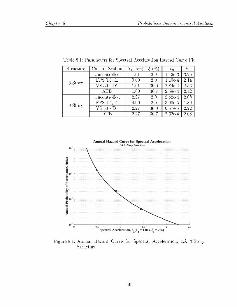
Chapter 8 Probabilistic Seismic Control Analysis
Table 8.1: Parameters for Spectral Acceleration Hazard Curve Fit
Structure Control System T1 (sec) � (%) k0 k1
3-Story
Uncontrolled 1.01 2.0 1.42e-3 3.25FPS T3, f1 3.00 2.0 1.10e-4 2.14VS 30 - D1 1.01 30.0 2.84e-4 2.33
ATB 1.00 36.7 2.59e-4 2.42
9-Story
Uncontrolled 2.27 2.0 2.62e-4 2.08FPS T4, f1 4.00 2.0 3.90e-5 1.89VS 30 - D1 2.27 30.0 6.67e-5 2.22
ATB 2.27 36.7 2.62e-4 2.08
0 0.5 1 1.5 2 2.510
−4
10−3
10−2
10−1
Annual Hazard Curce for Spectral Acceleration LA 3−Story Structure
Spectral Acceleration, Sa(T
1 = 1.01s, ξ
1 = 2%)
Ann
ual P
roba
bilit
y of
Exc
eeda
nce,
H(S
a)
Figure 8.1: Annual Hazard Curve for Spectral Acceleration, LA 3-StoryStructure
149

Probabilistic Seismic Control Analysis Chapter 8
0 0.2 0.4 0.6 0.8 1 1.2 1.4 1.6 1.8 210
−4
10−3
10−2
10−1
Annual Hazard Curce for Spectral Acceleration LA 9−Story Structure
Spectral Acceleration, Sa(T
1 = 2.3s, ξ
1 = 2%)
Ann
ual P
roba
bilit
y of
Exc
eeda
nce,
H(S
a)
Figure 8.2: Annual Hazard Curve for Spectral Acceleration, LA 9-StoryStructure
8.4 Relationship between Ground Motion and De-
mand Parameters
8.4.1 Estimate of Peak Story Drift
A functional relationship of the form given in Equation (8.8) can be �t to the data
by: 1) using the median values for Sa and Æmax for each hazard set, or 2) utilizing the
full data set of Sa and Æmax points. A linear regression of the log of the data selected
was performed to establish the parameters a and b. Regardless of whether the full
data set or only the median values were used in the regression the dispersion of Æmax
given Sa must be calculated as the square root of the mean squared deviation of the
full data set from the �tted curve, as shown below:
�ln(Æ)jSa = sqrt1
n� 2
nXi=1
�ln(Æ)� ln(�Æ)
�2(8.13)
150
Chapter 8 Probabilistic Seismic Control Analysis
where �Æ is the value of peak drift predicted from the �tted curve. The data was �tted
using both the full data set and the median values of the data. Plots of spectral
acceleration, Sa, versus the maximum story drift over the height of the structure,
Æmax, from the nonlinear dynamic analyses are presented in Figures 8.3 through 8.6.
The �t of the regression curve for the uncontrolled structure, shown in Figure 8.3,
displays a signi�cant amount of scatter to the �tted curve. Most of the contribution
to the scatter comes from the results of the 2 in 50 set of ground motions. The
resulting parameters for the regression �t to all the records are listed in Table 8.2.
When �tting through the median values, the resulting exponent coeÆcient, b, is only
slightly larger than 1, indicating a slight softening of the system. However, when the
�t is performed using the entire data set, the exponent b is signi�cantly smaller. This
trend proves to be consistent for all cases analyzed. One possible explanation lies in
the scaling procedure used. As discussed in Section 4.3, the earthquake records were
scaled to match speci�ed spectral acceleration valuea at four di�erent periods. As a
result, a record with a higher than average spectral acceleration value at the period on
interest to the structure is associated, by design, with spectral acceleration values that
are systematically lower than average at some of the other periods. As nonlinearities
occur, the period of the structure moves away from from the fundamental period and
into the range where the spectral acceleration is lower than average. So this record will
produce lower drifts than the \typical" records with the same spectral acceleration.
A reverse e�ect occurs with records with spectral accelerations lower than average
at the period of interest. The net result is a \ attening" of the �tted curve and
lower b values than might be expected from a random sample of record. Another
concern with this structure are the results due to the simmulated ground motions.
As discussed in Section 4.3, results due to the simulated, or synthetic, time histories
for structures with a period of 1 second can be misleading. Previous researchers have
found that to be true for this structure when determining the relationship between
spectral acceleration and drift (Luco and Cornell 1998). Results for the regression
analysis with no simulated records are also listed in Table 8.2 for the uncontrolled
structure. The dispersion given is now signi�cantly lower. Note, however that the
resulting �t is close to the original result. Both curve �ts are shown in Figure 8.3.
The relationship between ground motion and structural demand was analyzed
for the FPS isolation system with a 3 second isolation period and maximum fricion
151

Probabilistic Seismic Control Analysis Chapter 8
Table 8.2: Parameters for Fit of Relationship Between Spectral Accelerationand Story Drift, 3-Story Structure
Records Considered Fitted Data a b �ln(Æ)jSa
All Reccordsmedian 0.0291 1.099 0.383all 0.0288 0.842 0.346
No Simulatedmedian 0.0283 0.984 0.251all 0.0267 0.789 0.219
0 0.5 1 1.5 2 2.5 30
0.02
0.04
0.06
0.08
0.1
0.12
Drif
t Ang
le
Spectral Acceleration, Sa(T = 1.0s, ξ = 2%) [g]
Relationship between Spectral Acceleration and Peak Story Drift LA 3−Story Structure: α = 3%, no P−∆
50 in 50 Set
10 in 50 Set
2 in 50 Set
Fit: All
Fit: No Simulated
Figure 8.3: Relationship between Spectral Acceleration and Maximum PeakStory Drift for LA 3-Story Structure
152
Chapter 8 Probabilistic Seismic Control Analysis
coeÆcient of about 12% (FPS - T3, f1). The results of the regression analysis with the
response due to all records is listed in Table 8.3. As this system alternates between a
�xed base response, with a period of 1 second, and a sliding system, with a period of
3 seconds, analyses were performed with spectral acceleration values at both periods.
The resulting regression of the form in Equation (8.8) utilizing the median values
of each analysis set is poor, especially at high Sa values. Performing the regression
analysis utilizing all data points, rather than median values, provides only a small
bene�t, as indicated by the parameters in Table 8.3. Attempts to improve the �t
by determining Sa at the exact post-sliding period of 3.14 seconds or correlating to
another ground-motion parameter, such as the spectral velocity, had only a minimal
e�ect. The results also do not clearly indicate which parameters result in the better
�t.
The analyses were then performed ignoring the response of the simmulated, or
synthetic, time histories. The results, listed in Table 8.4, indicate signi�cantly re-
duced dispersion. Also, these results indicate that structural demand is more closely
associated with the spectral response at the �xed base period of 1 second. Utilizing
spectral velocity results in slightly less dispersion to the �tted curve. At low values
of Sa, the isolation system is not activated, as the horizontal forces observed by the
bearing are not greater than the frictional slip force of the bearing system. As a
result, the structure still has a fundamental period of 1 second and no reduction of
peak story drift is observed. Once the bearings begin to slide, the regression results
indicate a\hardening" relationship, where increases in Sa produce correspondingly
smaller changes in Æmax. This response results from the fact that the isolation bear-
ing limits the amount of force being transmitted to the superstructure. A comparison
of the regression �ts with and without the synthetic records is shown in Figure 8.4.
In contrast, the relationship between Sa and Æmax for the VS system is very strong,
as seen in Figure 8.5. The curve resulting from the regression �t is nearly linear, as
seen from the parameter b in Table 8.5 being nearly unity, and the scatter about the
curve is also low. One of the advantages of this result is that only a few number of
nonlinear dynamic analyses should be required to determine the functional relation-
ship between Sa and Æmax for this system. Also, this system is relatively una�ected
by the inclusion of the results from the simulated time histories.
153

Probabilistic Seismic Control Analysis Chapter 8
Table 8.3: Parameters for Fit of Relationship Between Spectral Value andStory Drift, 3-Story Structure with FPS Isolation System
Spectral Parameter Period Fitted Data a b �ln(Æ)jSa
Sa
1.0 secmedian 1.3 e-2 0.754 0.377all 1.2 e-2 0.525 0.348
3.0 secmedian 2.2 e-2 0.484 0.377all 2.0 e-2 0.380 0.291
3.14 secmedian 2.4 e-2 0.492 0.383all 2.0 e-2 0.381 0.372
Sv
1.0 secmedian 5.2 e-4 0.770 0.367all 1.3 e-3 0.549 0.341
3.0 secmedian 1.4 e-3 0.536 0.328all 1.7 e-3 0.483 0.326
Table 8.4: Parameters for Fit of Relationship Between Spectral Value andStory Drift, 3-Story Structure with FPS Isolation System - Ignor-ing Simulated Ground Motions
Spectral Parameter Period Fitted Data a b �ln(Æ)jSa
Sa
1.0 secmedian 1.2 e-2 0.567 0.216all 1.1 e-2 0.432 0.199
3.0 secmedian 1.8 e-2 0.378 0.324all 1.4 e-2 0.205 0.296
Sv
1.0 secmedian 1.1 e-3 0.567 0.201all 1.7 e-3 0.454 0.188
3.0 secmedian 1.9 e-3 0.434 0.281all 3.1 e-3 0.305 0.268
154

Chapter 8 Probabilistic Seismic Control Analysis
0 0.5 1 1.5 2 2.5 30
0.01
0.02
0.03
0.04
0.05
0.06
Drif
t Ang
le
Spectral Acceleration, Sa(T = 1.0s, ξ = 2%) [g]
Relationship between Spectral Acceleration and Peak Story Drift LA 3−Story Structure with FPS Isolation: α = 3%, no P−∆
50 in 50 Set
10 in 50 Set
2 in 50 Set
Fit: All
Fit: No Simulated
Figure 8.4: Relationship between Spectral Acceleration and Maximum PeakStory Drift for LA 3-Story Structure with FPS Isolation
A similar result is seen for the ATB system, shown in Figure 8.6, with little scat-
ter about the resulting curve, especially when compared to the uncontrolled results.
Though the scatter is a little higher than that of the viscous case, a much smaller
number of nonlinear dynamic analyses should be required to determine the functional
relationship between Sa and Æmax for this system. As these analyses can be extremely
computationally intensive, reducing the number of analyses required becomes a great
advantage. The resulting curve is essentially the same independent of whether the
simulated time histories are included, as indicated in Table 8.6.
Table 8.5: Parameters for Fit of Relationship Between Spectral Value andStory Drift for VS System
Records Considered �tted data a b �ln(Æ)jSa
All Reccordsmedian 2.97 e-2 1.10 0.132all 2.84 e-2 1.04 0.128
No Simulatedmedian 2.74 e-2 1.04 0.0978all 2.63 e-2 0.996 0.0935
155

Probabilistic Seismic Control Analysis Chapter 8
0 0.5 1 1.50
0.005
0.01
0.015
0.02
0.025
0.03
0.035
0.04
0.045
0.05
Drif
t Ang
le
Spectral Acceleration, Sa(T = 1.0s, ξ = 30%) [g]
Relationship between Spectral Acceleration and Peak Story Drift LA 3−Story Structure with VS Dampers: α = 3%, no P−∆
50 in 50 Set
10 in 50 Set
2 in 50 Set
Fit: All
Fit: No Simulated
Figure 8.5: Relationship between Spectral Acceleration and Maximum PeakStory Drift for LA 3-Story Structure with Viscous Brace System
0 0.5 1 1.50
0.01
0.02
0.03
0.04
0.05
0.06
0.07
Drif
t Ang
le
Spectral Acceleration, Sa(T = 1.0s, ξ = 36.7%) [g]
Relationship between Spectral Acceleration and Peak Story Drift LA 3−Story Structure with ATB System: α = 3%, no P−∆
50 in 50 Set
10 in 50 Set
2 in 50 Set
Fit: All
Fit: No Simulated
Figure 8.6: Relationship between Spectral Acceleration and Maximum PeakStory Drift for LA 3-Story Structure with ATB System
156

Chapter 8 Probabilistic Seismic Control Analysis
Table 8.6: Parameters for Fit of Relationship Between Spectral Value andStory Drift for ATB System
Records Considered �tted data a b �ln(Æ)jSa
All Reccordsmedian 3.31 e-2 1.02 0.287all 3.30 e-2 1.01 0.287
No Simulatedmedian 2.99 e-2 0.944 0.280all 2.98 e-2 0.943 0.280
8.4.2 Estimate of Control System Demand
An estimate of the demand on the control system can also be determined using a
similar process. For the viscous dampers, the dependence between the peak force in
the damper and the spectral acceleration is taken to be:
FD = aSba (8.14)
where FD is the peak damper force. This relationship is essentially the same as that
for peak drift, given in Equation (8.8). The regression results are listed in Table 8.7
for the VS damper systems for 20%, 30%, and 40% e�ective damping using equal
sized dampers in every story.
Table 8.7: Parameters for Fit of Relationship Between Spectral Value andPeak Damper Force
E�ective Damping �tted data a b �ln(Æ)jSx20% all 825 0.761 0.1930% all 1,122 0.786 0.2040% all 1,326 0.793 0.21
For the FPS isolation system, the displacement of the bearings can be consid-
ered as a drift-type quantity. As a result, a similar relationship as that given in
Equation (8.8) can be developed for the beak bearing displacement as shown below:
ÆB = aSbx (8.15)
where ÆB is the peak bearing displacement and Sx represents any spectral quantity
of interest. Both spectral acceleration, Sa, and spectral velocity, Sv, at the isolation
157
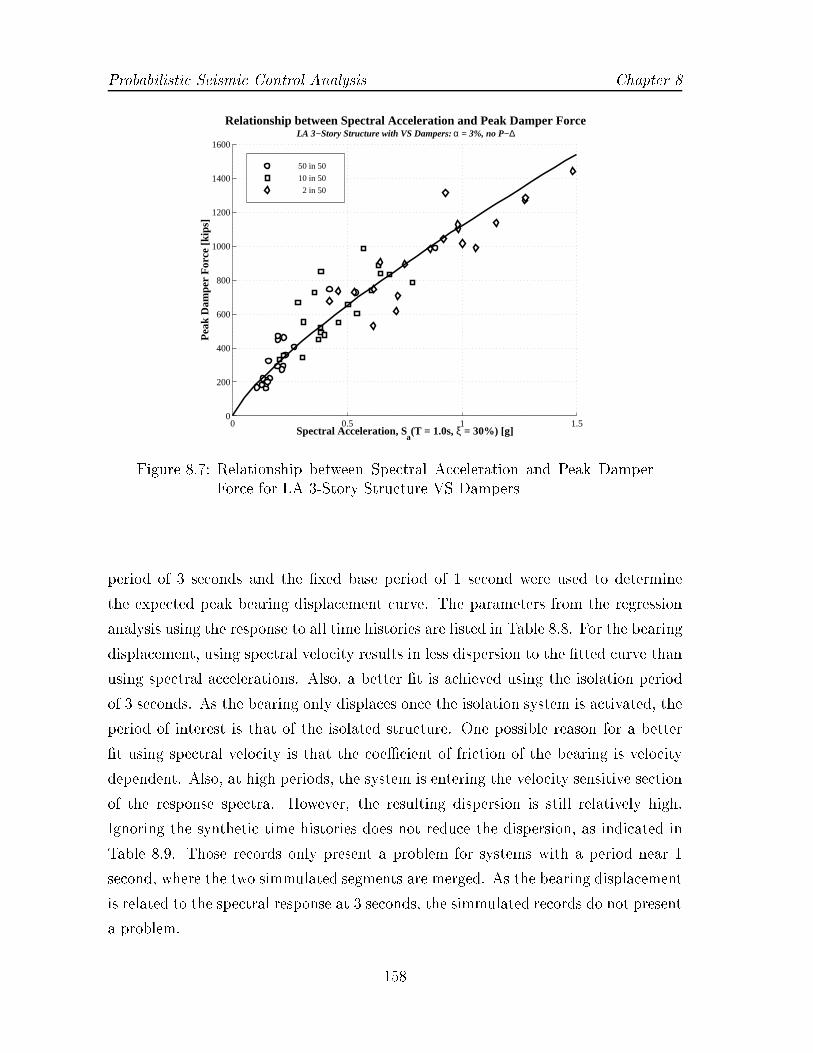
Probabilistic Seismic Control Analysis Chapter 8
0 0.5 1 1.50
200
400
600
800
1000
1200
1400
1600
Pea
k D
ampe
r F
orce
[kip
s]
Spectral Acceleration, Sa(T = 1.0s, ξ = 30%) [g]
Relationship between Spectral Acceleration and Peak Damper Force LA 3−Story Structure with VS Dampers: α = 3%, no P−∆
50 in 50
10 in 50
2 in 50
Figure 8.7: Relationship between Spectral Acceleration and Peak DamperForce for LA 3-Story Structure VS Dampers
period of 3 seconds and the �xed base period of 1 second were used to determine
the expected peak bearing displacement curve. The parameters from the regression
analysis using the response to all time histories are listed in Table 8.8. For the bearing
displacement, using spectral velocity results in less dispersion to the �tted curve than
using spectral accelerations. Also, a better �t is achieved using the isolation period
of 3 seconds. As the bearing only displaces once the isolation system is activated, the
period of interest is that of the isolated structure. One possible reason for a better
�t using spectral velocity is that the coeÆcient of friction of the bearing is velocity
dependent. Also, at high periods, the system is entering the velocity sensitive section
of the response spectra. However, the resulting dispersion is still relatively high.
Ignoring the synthetic time histories does not reduce the dispersion, as indicated in
Table 8.9. Those records only present a problem for systems with a period near 1
second, where the two simmulated segments are merged. As the bearing displacement
is related to the spectral response at 3 seconds, the simmulated records do not present
a problem.
158

Chapter 8 Probabilistic Seismic Control Analysis
Table 8.8: Parameters for Fit of Relationship Between Spectral Value andPeak Bearing Displacement, 3-Story Structure with FPS IsolationSystem
Spectral Parameter Period Fitted Data a b �ln(Æ)jSx
Sa
1.0 secmedian 7.08 2.252 0.809all 6.24 1.529 0.668
3.0 secmedian 41.44 1.472 0.755all 25.68 1.146 0.706
Sv
1.0 secmedian 5.7 e-4 2.268 0.809all 0.0098 1.553 0.678
3.0 secmedian 0.0080 1.622 0.534all 0.0161 1.441 0.517
Table 8.9: Parameters for Fit of Relationship Between Spectral Value andPeak Bearing Displacement, 3-Story Structure with FPS IsolationSystem - No Simulated Records
Spectral Parameter Period Fitted Data a b �ln(Æ)jSx
Sa
1.0 secmedian 6.43 2.076 0.707all 5.45 1.433 0.582
3.0 secmedian 38.17 1.432 0.806all 19.19 1.016 0.743
Sv
1.0 secmedian 0.0012 2.055 0.704all 0.0132 1.449 0.598
3.0 secmedian 0.0077 1.629 0.578all 0.0192 1.389 0.556
159

Probabilistic Seismic Control Analysis Chapter 8
0 0.1 0.2 0.3 0.4 0.5 0.6 0.7 0.8 0.9 10
5
10
15
20
25
30
35
40
Pea
k B
earin
g D
ispl
acem
ent [
inch
es]
Spectral Acceleration, Sa(T = 3.0s, ξ = 2%) [g]
Relationship between Spectral Acceleration and Peak Story Dr if t LA 3−Story Structure with FPS Isolation: α = 3%, no P−∆
50 in 50
10 in 50
2 in 50
Figure 8.8: Relationship between Spectral Acceleration and Peak BearingDisplacement for LA 3-Story Structure FPS Isolation
0 20 40 60 80 100 120 140 160 180 2000
5
10
15
20
25
30
35
40
Pea
k B
earin
g D
ispl
acem
ent [
inch
es]
Spectral Velocity, Sv(T = 3.0s, ξ = 2%) [in/sec]
Relationship between Spectral Velocity and Maximum Bearing Displacement LA 3−Story Structure with FPS Isolation: α = 3%, no P−∆
50 in 50
10 in 50
2 in 50
Figure 8.9: Relationship between Spectral Velocity and Peak Bearing Dis-placement for LA 3-Story Structure FPS Isolation
160

Chapter 8 Probabilistic Seismic Control Analysis
8.4.3 Number of Analyses
The required minimum number of simulations, n, can be determined based on the
estimation error of the median demand, which is expressed as a fraction of the median.
The standard error, �ln Æ, due to the use of a limited sample size is approximately equal
to:
�ln Æ =�ln(Æ)jSap
n
1 +
ln(Sa)� ln( �Sa)
�2ln(Sa)
!
� �ln(Æ)jSapn
(8.16)
for Sa � Sa. This relationship is illustrated in Figure 8.10 for all four systems. In all
cases, 20 analyses ensure that the one-sigma con�dence band on the estimation of the
median peak drift demand lying within 10% of the median value. The VS and ATB
systems require signi�cantly fewer analyses, with the VS system having a one-sigma
con�dence band within 10% of the median with only 3 analyses.
0 10 20 30 40 50 600
0.05
0.1
0.15
0.2
0.25
0.3
0.35
0.4
Standard Error in Estimation due to Limited Sample Size LA 3−Story Structure: Regression on All Data Points
Number of Analyses
Sta
ndar
d E
rror
Uncontrolled
FPS − T3, f1
VS − 30, D1
ATB − S1k
Figure 8.10: Standard Error in Peak Drift Estimation due to Limited SampleSize Using Full Data Set, 3-Story Structure
161

Probabilistic Seismic Control Analysis Chapter 8
8.5 Drift Demand Hazard Curves
Once the median relationship between spectral acceleration and drift (i.e., the median
drift given spectral acceleration), and the dispersion of drift given spectral acceleration
are known, the spectral acceleration hazard curve can be used to create a drift demand
hazard curve. Median values are used as the ground motion sets were developed to
be used as a unit, so that the seismic demand for a structure for a given hazard is
best approximated by the median response. The resulting drift demand curves can be
used to determine the impact of control parameter design as well as provide a basis
for comparison between systems.
8.5.1 E�ect of Control Parameter Variation
Interstory drift demand hazard curves were developed for the FPS isolation system
with sliding surface f1 and isolation periods of 2, 3, and 4 seconds. The parameters
utilized in generating these curves are listed in Table 8.10. In Section 6.3.1, increasing
the isolation period is shown to cause a decrease in the median values of peak inter-
story drift demands, especially at the high hazard level. Consequently, increasing
the isolation period results in a decrease in the probability of exceeding a given drift
demand. However, the slopes of the 3 curves are signi�cantly di�erent, so that the dif-
ferences between the systems increases for higher target drifts. One major reason for
this result lies in the impact on the response scatter associated with each system. As
the isolation period increases, the scatter in the seismic demand response decreases,
resulting in a decrease in the uncertainty associated with that parameter. Also, the
e�ect of increasing isolation period was demonstrated to be more signi�cant for the 2
in 50 set, or high hazard level, than for lower seismic hazards, since a minimal force
must be generated across the sliding surface before the isolation system is triggered.
Similarly, maximum peak story drift hazard curves were developed for VS damp-
ing systems with di�erent e�ective damping values and are shown in Figure 8.12.
Increasing the damping in the system corresponds the expectation that higher damp-
ing values reduce drift demands and, therefore, the probability of exceeding a target
drift level. Increasing the e�ective damping in the system produces a fairly even shift
downwards of the curve over the range of return periods considered. Maximum peak
162
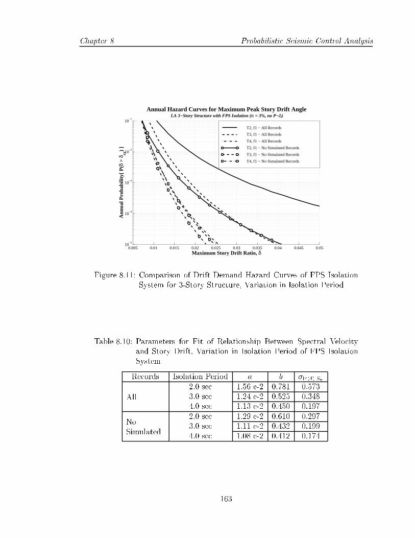
Chapter 8 Probabilistic Seismic Control Analysis
0.005 0.01 0.015 0.02 0.025 0.03 0.035 0.04 0.045 0.0510
−5
10−4
10−3
10−2
10−1
Maximum Story Drift Ratio, δ
Ann
ual P
roba
bilit
y[ P
(δ >
δcr
) ]
Annual Hazard Curves for Maximum Peak Story Drift Angle LA 3−Story Structure with FPS Isolation (α = 3%, no P−∆)
T2, f1 − All Records
T3, f1 − All Records
T4, f1 − All Records
T2, f1 − No Simulated Records
T3, f1 − No Simulated Records
T4, f1 − No Simulated Records
Figure 8.11: Comparison of Drift Demand Hazard Curves of FPS IsolationSystem for 3-Story Structure, Variation in Isolation Period
Table 8.10: Parameters for Fit of Relationship Between Spectral Velocityand Story Drift, Variation in Isolation Period of FPS IsolationSystem
Records Isolation Period a b �ln(Æ)jSv
All
2.0 sec 1.56 e-2 0.781 0.5733.0 sec 1.24 e-2 0.525 0.3484.0 sec 1.13 e-2 0.450 0.197
NoSimulated
2.0 sec 1.29 e-2 0.610 0.2973.0 sec 1.11 e-2 0.432 0.1994.0 sec 1.08 e-2 0.412 0.174
163
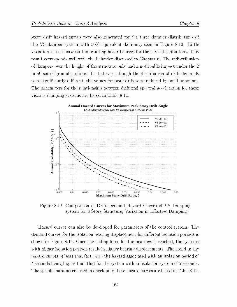
Probabilistic Seismic Control Analysis Chapter 8
story drift hazard curves were also generated for the three damper distributions of
the VS damper system with 30% equivalent damping, seen in Figure 8.13. Little
variation is seen between the resulting hazard curves for the three distributions. This
result corresponds well with the behavior discussed in Chapter 6. The redistribution
of dampers over the height of the structure only had a noticeable impact under the 2
in 50 set of ground motions. In that case, though the distribution of drift demands
were signi�cantly di�erent, the values for peak drift were reduced by small amounts.
The parameters for the relationship between drift and spectral acceleration for these
viscous damping systems are listed in Table 8.11.
0.005 0.01 0.015 0.02 0.025 0.03 0.035 0.04 0.045 0.0510
−4
10−3
10−2
10−1
Maximum Story Drift Ratio, δ
Ann
ual P
roba
bilit
y[ P
(δ >
δcr
) ]
Annual Hazard Curves for Maximum Peak Story Drift Angle LA 3−Story Structure with VS Dampers (α = 3%, no P−∆)
VS 20 − D1
VS 30 − D1
VS 40 − D1
Figure 8.12: Comparison of Drift Demand Hazard Curves of VS Dampingsystem for 3-Story Structure, Variation in E�ective Damping
Hazard curves can also be developed for parameters of the control system. The
demand curves for the isolation bearing displacement for di�erent isolation periods is
shown in Figure 8.14. Once the sliding force for the bearings is reached, the systems
with higher isolation periods result in higher bearing displacements. The trend in the
hazard curves re ects that fact, with the hazard associated with an isolation period of
4 seconds being higher than that for the system with an isolation system of 2 seconds.
The speci�c parameters used in developing these hazard curves are listed in Table 8.12.
164
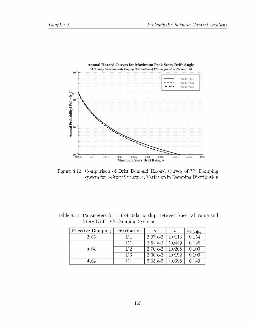
Chapter 8 Probabilistic Seismic Control Analysis
0.005 0.01 0.015 0.02 0.025 0.03 0.035 0.04 0.045 0.0510
−4
10−3
10−2
10−1
Maximum Story Drift Ratio, δ
Ann
ual P
roba
bilit
y[ P
(δ >
δcr
) ]
Annual Hazard Curves for Maximum Peak Story Drift Angle LA 3−Story Structure with Varying Distribution of VS Dampers (α = 3%, no P−∆)
VS 30 − D1
VS 30 − D2
VS 30 − D3
Figure 8.13: Comparison of Drift Demand Hazard Curves of VS Dampingsystem for 3-Story Structure, Variation in Damping Distribution
Table 8.11: Parameters for Fit of Relationship Between Spectral Value andStory Drift, VS Damping Systems
E�ective Damping Distribution a b �ln(Æ)jSa20% D1 2.97 e-2 1.0113 0.154
30%
D1 2.84 e-2 1.0449 0.128D2 2.70 e-2 1.0208 0.103D3 2.66 e-2 1.0192 0.109
40% D1 2.63 e-2 1.0698 0.149
165

Probabilistic Seismic Control Analysis Chapter 8
A second set of hazard curves were developed by developing a relationship between
bearing displacement and spectral velocity, Sv, evaluated at the isolation period. This
�t of the data results in less scatter from the �tted curve, as seen from the values of
�ln(Æ)jSv . The hazard curves are much atter than those developed using Sa, so that
the hazard at low bearing displacements is noticeably lower. A word of caution must
be made regarding the hazard curves developed using Sv. The assumption is made
that the hazard for the median spectral velocity of each ground motion set is the
same as the hazard for spectral acceleration of the corresponding ground motion set.
Since the sets were developed for spectral acceleration hazard, this assumption may
not be true and should be veri�ed.
5 10 15 20 25 30 35 4010
−4
10−3
10−2
Maximum Bearing Displacement
Ann
ual P
roba
bilit
y [ P
( θ
> θ
cr )
]
Annual Hazard Curves for Maximum Bearing Displacement 3−Story Structure
FPS − T2, f1
FPS − T3, f1
FPS − T4, f1
Figure 8.14: Comparison of Bearing Displacement Demand Hazard Curvesfor 3-Story Structure, Variation in Isolation Period
These drift hazard curves can be used in the design process of the control system.
With this information, optimization of the control design for the structural system
can be accomplished over a range of seismic hazards.
166

Chapter 8 Probabilistic Seismic Control Analysis
Table 8.12: Parameters for Fit of Relationship Between Spectral Value andBearing Displacements, Variation in Isolation Period of FPS Iso-lation System
Isolation Period �tted data Spectral Parameter a b �ln(Æ)jS
T = 2.0 sec allSa 13.0 1.168 0.517Sv 0.020 1.345 0.405
T = 3.0 sec allSa 25.7 1.142 0.706Sv 0.016 1.445 0.403
T = 4.0 sec allSa 35.5 0.961 0.840Sv 0.027 1.368 0.617
5 10 15 20 25 30 35 4010
−4
10−3
10−2
Maximum Bearing Displacement
Ann
ual P
roba
bilit
y [ P
( θ
> θ
cr )
]
Annual Hazard Curves for Maximum Bearing Displacement 3−Story Structure
FPS − T2, f1
FPS − T3, f1
FPS − T4, f1
Figure 8.15: Comparison of Bearing Displacement Demand Hazard Curvesfor 3-Story Structure, Variation in Isolation Period
167

Probabilistic Seismic Control Analysis Chapter 8
8.5.2 Comparison Between Control Systems
This probabilistic performance assessment can also be utilized to compare the per-
formance of di�erent control strategies for the same structural system. The curves
showing the maximum interstory drift hazard for each of the control strategies dis-
cussed in Section 6.4 for the 3-Story structure are plotted in Figure 8.16. All three
control strategies result in signi�cant reductions in drift hazard. However, no single
strategy proves to be most e�ective at all target drift limits. The drift hazard for the
VS damper system and ATB system are very similar over the drift range considered.
The VS system has a smaller drift hazard over this range; however, the two curves
begin to converge at the high end. The FPS isolation drift hazard curve crosses both
other controlled drift hazard curves, exhibiting higher drift hazard at low return peri-
ods and lower drift hazard at high return periods. This condition re ects the fact that
frictional isolation systems only impact the structural response if the forces through
the bearing are large enough to overcome the frictional slip force for the bearing. The
other factor a�ecting the performance of the FPS system with respect to the two
other control systems is the scatter in the structural response for a given spectral
acceleration.
Similar curves were developed for the control strategies designed for the 9-Story
structure, shown in Figure 8.17. Again, though all three control strategies reduce
the drift hazard, no one strategy is the most e�ective at all return periods or target
drift levels. The ATB system is consistently less e�ective than the two passive control
system. However, recall that this system only utilizes 3 braces located at the �rst,
second, and eighth stories, and as such has a much smaller capacity than the VS
system plotted here. The drift hazard curves for the FPS isolation VS systems cross
at a drift limit of about 3%. The VS system has a lower drift hazard at the low return
periods, while the FPS isolation has a lower drift hazard at higher return periods.
One of the disadvantages of utilizing the maximum peak story drift over the height
of the structure is the loss of the location of the critical points in the structure. Also,
the location of the maximum peak story drift is not the same for all analyses of a
given system, much less across systems. For di�erent systems, peak drift locations
may be completely di�erent. However, drift hazard curves can be developed for
individual stories. Then, for a given story, a probabilistic performance assessment
168
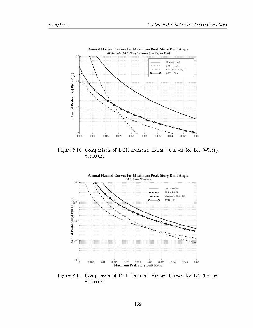
Chapter 8 Probabilistic Seismic Control Analysis
0.005 0.01 0.015 0.02 0.025 0.03 0.035 0.04 0.045 0.0510
−4
10−3
10−2
10−1
Ann
ual P
roba
bilit
y[ P
(δ >
δcr
) ]
Annual Hazard Curves for Maximum Peak Story Drift Angle All Records: LA 3−Story Structure (α = 3%, no P−∆)
Uncontrolled FPS − T3, f1 Viscous − 30%, D1ATB − S1k
Figure 8.16: Comparison of Drift Demand Hazard Curves for LA 3-StoryStructure
0 0.005 0.01 0.015 0.02 0.025 0.03 0.035 0.04 0.045 0.0510
−5
10−4
10−3
10−2
10−1
Maximum Peak Story Drift Ratio
Ann
ual P
roba
bilit
y[ P
(θ >
θcr
) ]
Annual Hazard Curves for Maximum Peak Story Drift Angle LA 9−Story Structure
Uncontrolled
FPS − T4, f1
Viscous − 30%, D1
ATB − S1k
Figure 8.17: Comparison of Drift Demand Hazard Curves for LA 9-StoryStructure
169
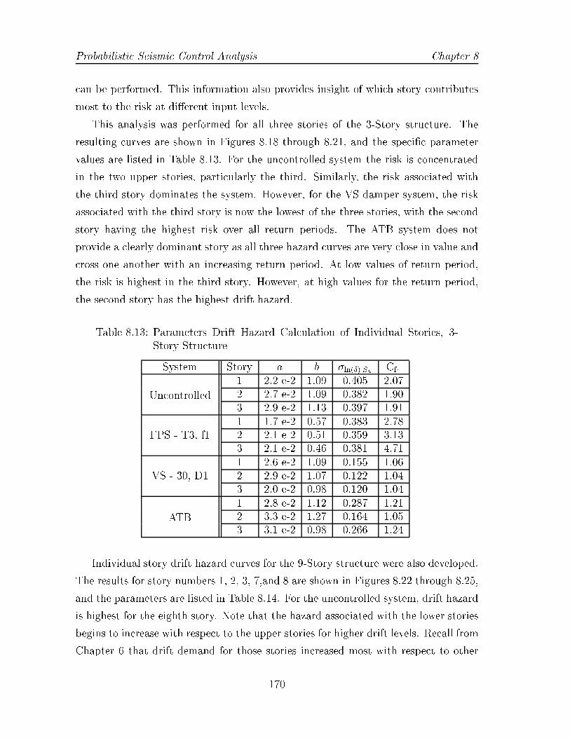
Probabilistic Seismic Control Analysis Chapter 8
can be performed. This information also provides insight of which story contributes
most to the risk at di�erent input levels.
This analysis was performed for all three stories of the 3-Story structure. The
resulting curves are shown in Figures 8.18 through 8.21, and the speci�c parameter
values are listed in Table 8.13. For the uncontrolled system the risk is concentrated
in the two upper stories, particularly the third. Similarly, the risk associated with
the third story dominates the system. However, for the VS damper system, the risk
associated with the third story is now the lowest of the three stories, with the second
story having the highest risk over all return periods. The ATB system does not
provide a clearly dominant story as all three hazard curves are very close in value and
cross one another with an increasing return period. At low values of return period,
the risk is highest in the third story. However, at high values for the return period,
the second story has the highest drift hazard.
Table 8.13: Parameters Drift Hazard Calculation of Individual Stories, 3-Story Structure
System Story a b �ln(Æ)jSa Cf1
Uncontrolled
1 2.2 e-2 1.09 0.405 2.072 2.7 e-2 1.09 0.382 1.903 2.9 e-2 1.13 0.397 1.91
FPS - T3, f11 1.7 e-2 0.57 0.383 2.782 2.1 e-2 0.51 0.359 3.133 2.1 e-2 0.46 0.381 4.71
VS - 30, D11 2.6 e-2 1.09 0.155 1.062 2.9 e-2 1.07 0.122 1.043 2.0 e-2 0.98 0.120 1.04
ATB
1 2,8 e-2 1.12 0.287 1.212 3.3 e-2 1.27 0.164 1.053 3.1 e-2 0.98 0.266 1.24
Individual story drift hazard curves for the 9-Story structure were also developed.
The results for story numbers 1, 2, 3, 7,and 8 are shown in Figures 8.22 through 8.25,
and the parameters are listed in Table 8.14. For the uncontrolled system, drift hazard
is highest for the eighth story. Note that the hazard associated with the lower stories
begins to increase with respect to the upper stories for higher drift levels. Recall from
Chapter 6 that drift demand for those stories increased most with respect to other
170

Chapter 8 Probabilistic Seismic Control Analysis
0 0.005 0.01 0.015 0.02 0.025 0.03 0.035 0.04 0.045 0.0510
−5
10−4
10−3
10−2
10−1
Maximum Story Drift Ratio
Ann
ual P
roba
bilit
y[ P
(θ >
θcr
) ]
Annual Hazard Curves for Peak Story Drift Angle LA 3−Story Structure: α = 3%, no P−∆
First Story
Second Story
Third Story
Figure 8.18: Comparison of Individual Story Drift Demand Hazard Curvesfor LA 3-Story Structure
0 0.005 0.01 0.015 0.02 0.025 0.03 0.035 0.04 0.045 0.0510
−5
10−4
10−3
10−2
10−1
Maximum Story Drift Ratio
Ann
ual P
roba
bilit
y[ P
(θ >
θcr
) ]
Annual Hazard Curves for Peak Story Drift Angle LA 3−Story Structure: α = 3%, no P−∆
First Story
Second Story
Third Story
Figure 8.19: Comparison of Individual Story Drift Demand Hazard Curvesfor LA 3-Story Structure with FPS Isolation
171
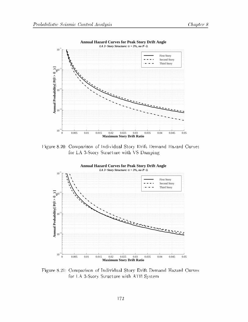
Probabilistic Seismic Control Analysis Chapter 8
0 0.005 0.01 0.015 0.02 0.025 0.03 0.035 0.04 0.045 0.0510
−5
10−4
10−3
10−2
10−1
Maximum Story Drift Ratio
Ann
ual P
roba
bilit
y[ P
(θ >
θcr
) ]
Annual Hazard Curves for Peak Story Drift Angle LA 3−Story Structure: α = 3%, no P−∆
First Story
Second Story
Third Story
Figure 8.20: Comparison of Individual Story Drift Demand Hazard Curvesfor LA 3-Story Structure with VS Damping
0 0.005 0.01 0.015 0.02 0.025 0.03 0.035 0.04 0.045 0.0510
−5
10−4
10−3
10−2
10−1
Maximum Story Drift Ratio
Ann
ual P
roba
bilit
y[ P
(θ >
θcr
) ]
Annual Hazard Curves for Peak Story Drift Angle LA 3−Story Structure: α = 3%, no P−∆
First Story
Second Story
Third Story
Figure 8.21: Comparison of Individual Story Drift Demand Hazard Curvesfor LA 3-Story Structure with ATB System
172

Chapter 8 Probabilistic Seismic Control Analysis
stories when comparing the drift demands from the 10 in 50 set and the 50 in 50 set.
This same phenomenon is illustrated here.
Table 8.14: Parameters Drift Hazard Calculation of Individual Stories, 9-Story Structure
System Story a b �ln(Æ)jSa Cf1
Uncontrolled
1 4.5 e-2 0.63 0.242 2.782 4.3 e-2 0.84 0.240 3.133 4.6 e-2 0.89 0.253 3.137 3.3 e-2 0.57 0.293 3.138 3.9 e-2 0.56 0.357 4.71
FPS - T4, f1
1 4.2 e-2 0.61 0.379 1.982 3.5 e-2 0.76 0.412 1.683 3.6 e-2 0.77 0.399 1.617 2.4 e-2 0.47 0.371 3.038 2.7 e-2 0.44 0.385 3.83
VS 30, D1
1 6.6 e-2 0.63 0.242 1.372 5.5 e-2 0.84 0.239 1.193 5.1 e-2 0.89 0.253 1.197 2.4 e-2 0.57 0.293 1.758 1.9 e-2 0.56 0.357 2.36
ATB
1 3.8 e-2 1.01 0.139 1.052 3.8 e-2 1.11 0.132 1.043 4.3 e-2 1.09 0.129 1.047 3.1 e-2 0.99 0.126 1.058 3.8 e-2 0.99 0.128 1.05
The drift hazard curves for the 9-Story structure with FPS isolation system is
shown in Figure 8.23. At low return periods the drift hazard is highest for the upper
stories. As the return periods increase, the drift hazard becomes dominated by the
lower stories.
The 9-Story structure with VS dampers maintains relationship between stories
constant for the hazard range of interest, as seen in Figure 8.24. The highest drift
hazard is consistently associated with the �rst story, and the lowest drift hazard is
consistently associated with the uppermost story. This phenomenon was also observed
in the seismic story demand plots for individual ground motion sets, where a constant
decrease in drift demands was observed as one went up the structure.
The individual story drift hazard curves for the 9-Story structure with ATB are
173

Probabilistic Seismic Control Analysis Chapter 8
0 0.005 0.01 0.015 0.02 0.025 0.03 0.035 0.04 0.045 0.0510
−5
10−4
10−3
10−2
10−1
Maximum Story Drift Ratio
Ann
ual P
roba
bilit
y[ P
(θ >
θcr
) ]
Annual Hazard Curves for Peak Story Drift Angle LA 9Story Structure: α = 3%, no P−∆
First Story
Second Story
Third Story
Seventh Story
Eigth Story
Figure 8.22: Comparison of Individual Story Drift Demand Hazard Curvesfor LA 9-Story Structure
0 0.005 0.01 0.015 0.02 0.025 0.03 0.035 0.04 0.045 0.0510
−5
10−4
10−3
10−2
10−1
Maximum Story Drift Ratio
Ann
ual P
roba
bilit
y[ P
(θ >
θcr
) ]
Annual Hazard Curves for Peak Story Drift Angle LA 9Story Structure with FPS Isolation − T4, f1: α = 3%, no P−∆
First Story
Second Story
Third Story
Seventh Story
Eigth Story
Figure 8.23: Comparison of Individual Story Drift Demand Hazard Curvesfor LA 9-Story Structure with FPS Isolation
174
Chapter 8 Probabilistic Seismic Control Analysis
0.005 0.01 0.015 0.02 0.025 0.03 0.035 0.04 0.045 0.0510
−5
10−4
10−3
10−2
10−1
Maximum Story Drift Ratio
Ann
ual P
roba
bilit
y[ P
(θ >
θcr
) ]
Annual Hazard Curves for Peak Story Drift Angle LA 9Story Structure: α = 3%, no P−∆
First Story
Second Story
Third Story
Seventh Story
Eigth Story
Figure 8.24: Comparison of Individual Story Drift Demand Hazard Curvesfor LA 9-Story Structure with VS Damping
plotted in Figure 8.25. The curves for all the stories lie very close to one another and
no clear trend exists as to which stories have the highest drift hazard. The controller
was designed with equal weighting placed on all story drift values, resulting in an
\evening out" of the drift hazard over the height.
8.6 Conclusions
Current performance guidelines provide for the determination of seismic demands
for a given scenario event, which is then compared with an allowable limit. These
procedures do not account for the variability in seismic demand estimation. One
approach to address this issue is the development of probabilistic seismic demand
curves. This study uses the methodology developed by (Cornell 1996) that combines
information regarding the seismic hazard and nonlinear structural response. The
procedure relates a record speci�c quantity, such as the elastic spectral acceleration, to
a structural response parameter, such as drift, to estimate the probability of exceeding
the selected structural parameter.
175
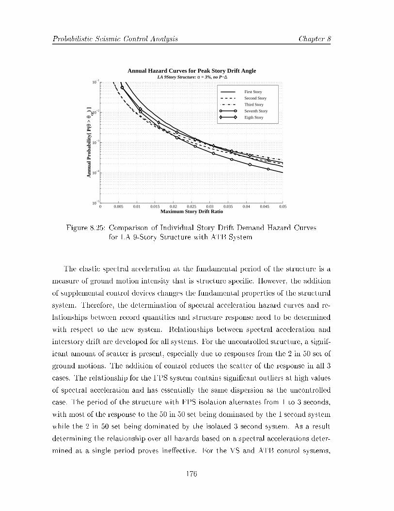
Probabilistic Seismic Control Analysis Chapter 8
0 0.005 0.01 0.015 0.02 0.025 0.03 0.035 0.04 0.045 0.0510
−5
10−4
10−3
10−2
10−1
Maximum Story Drift Ratio
Ann
ual P
roba
bilit
y[ P
(θ >
θcr
) ]
Annual Hazard Curves for Peak Story Drift Angle LA 9Story Structure: α = 3%, no P−∆
First Story
Second Story
Third Story
Seventh Story
Eigth Story
Figure 8.25: Comparison of Individual Story Drift Demand Hazard Curvesfor LA 9-Story Structure with ATB System
The elastic spectral acceleration at the fundamental period of the structure is a
measure of ground motion intensity that is structure speci�c. However, the addition
of supplemental control devices changes the fundamental properties of the structural
system. Therefore, the determination of spectral acceleration hazard curves and re-
lationships between record quantities and structure response need to be determined
with respect to the new system. Relationships between spectral acceleration and
interstory drift are developed for all systems. For the uncontrolled structure, a signif-
icant amount of scatter is present, especially due to responses from the 2 in 50 set of
ground motions. The addition of control reduces the scatter of the response in all 3
cases. The relationship for the FPS system contains signi�cant outliers at high values
of spectral acceleration and has essentially the same dispersion as the uncontrolled
case. The period of the structure with FPS isolation alternates from 1 to 3 seconds,
with most of the response to the 50 in 50 set being dominated by the 1 second system
while the 2 in 50 set being dominated by the isolated 3 second system. As a result
determining the relationship over all hazards based on a spectral accelerations deter-
mined at a single period proves ine�ective. For the VS and ATB control systems,
176

Chapter 8 Probabilistic Seismic Control Analysis
the scatter is greatly reduced. This fact implies that a smaller number of analyses
could be used to determine the relationship between drift and spectral accelerations.
Estimates on the error associated with the estimate of the system demand indicate
that signi�cantly fewer analyses could have been used. As control analyses can be
computationally intensive, reducing the number of required analyses becomes a great
advantage to the designer.
Once this information is combined with the spectral hazard, the resulting demand
hazard curves can be used to compare the e�ects of di�erent parameters for a single
control type as well as the performance between the di�erent control strategies. Re-
sults from these curves indicate that no single control strategy is the most e�ective
at all hazard levels. For example, at low return periods the VS system has the lowest
drift demands. However, at higher return periods, the FPS isolation system becomes
the most e�ective strategy.
177
Chapter 9
Summary, Conclusions, and
Future Work
9.1 Summary
The structural engineering community has been making great strides in recent years
to develop performance-based earthquake engineering methodologies for both new
and existing construction. Both SEAOC's Vision 2000 projects and BSSC's NEHRP
Guidelines for Seismic Rehabilitation of Buildings present the �rst guidelines for
multi-level performance objectives. One of the intents of these provisions is to pro-
vide methods for designing and evaluating structures such that they are capable of
providing predictable performance during an earthquake.
Structural control can provide an additional method to meet desired performance
objectives. Design of a structure/controller system should involve a thorough un-
derstanding of how various types of controllers enhance structural performance, such
that the most e�ective type of controller is selected for the given structure and seismic
hazard. Controllers may be passive, requiring no external energy source, or active,
requiring an external power source.
The goal of the research presented here is to evaluate the role of structural con-
trol technology in enhancing the overall structural performance under seismic ex-
citations. This investigation has the following speci�c objectives: (1) To evaluate
the e�ect of the various controller architectures on seismic demands as described
through performance-based design criteria; (2) To evaluate the sensitivity of the
178
Chapter 9 Summary, Conclusions, and Future Work
structure/controller performance based variation of control parameters, load levels
and structural modeling techniques; and (3) To compare the bene�ts of the con-
trollers in both a deterministic and probabilistic format. This study focuses on steel
moment resisting frames and three types of possible controllers: (1) base isolation
system (passive); (2) linear viscous brace dampers (passive); and (3) active tendon
braces. Two structures are selected from the SAC Phase II project, the three story
system and the nine story system. Simulations of these systems, both controlled and
uncontrolled, are prepared using the three suites of earthquake records, also from the
SAC Phase II project, representing three return di�erent periods. Several controllers
are developed for each structure, and their performance is judged based on the drift,
dissipated hysteretic energy, and oor acceleration demands.
9.2 Results
9.2.1 Seismic Demands
Comparisons of the performance of three di�erent control strategies are presented for
all three sets of ground motions. The comparison is based on story drift, hysteretic
energy, and oor acceleration demands. All three controllers were successful in reduc-
ing the seismic demands, though no one system is consistently better than the others
at all hazard levels. For story drift demands, the values suggested for peak story drift
angles in FEMA 273 are used as guidelines for judging structural performance.
For short return periods, the addition of structural control reduced the median
story drift by nearly 50%. In the 10 in 50 ground motion set, the median response
of the uncontrolled system lies just below the life-safety limit of 2.5% drift. Several
individual records push the uncontrolled response beyond the collapse prevention limit
of 5% The application of control is e�ective in reducing both the median response and
its scatter, with the median response falling at about 1% drift for all three control
systems. The most signi�cant impact of control occurs with the 2 in 50 ground
motions. The uncontrolled structure has a median response just under the collapse
prevention limit. Clear outliers are present in the data, with some response values
exceeding 10% drift that are unsustainable by the physical system. The ATB and
VS control systems bring the median drift response to about 3%, with the VS system
179
Summary, Conclusions, and Future Work Chapter 9
resulting in less scatter in the data. The FPS isolation has the lowest median response,
with values of about 1.5%. However, noticeable outliers are present in the data, with
a couple of records having demands close to the collapse limit.
Results for the 9-story structure follow a similar trend as those of the 3-story
structure. Both the VS and FPS isolation are extremely e�ective at reducing the
peak story drift demands. The VS system proves to be most e�ective at higher
stories, while the FPS system is slightly less e�ective at the upper stories. For the
ATB control system, the actuators are placed on only the 1st, 2nd, and 8th stories.
The e�ect of this placement is that at high level excitations the drift demands at
stories without actuators are increased from the uncontrolled case. For comparison,
a VS system with dampers in only the same three stories and comparable peak forces
was designed. The resulting peak story drift demands were higher than those of
the uncontrolled structure in those stories lacking dampers. In contrast, if smaller
dampers are added at every story to produce the same amount of e�ective damping,
signi�cant reductions in drift result for all stories.
Residual drift values are used by FEMA 273 as an indicator of the inelastic damage
to the structural system. However, care must be taken in interpreting these values as
they can be misleading. In both the 50 in 50 set and 10 in 50 set of ground motions,
the median values for residual drifts of the control systems are close to negligible.
However, in the 2 in 50 set of ground motions, median values for all systems are
signi�cantly higher. The addition of the two passive controls decreases the median
drift demand value. However, the median value for the ATB system is greater than
that for the uncontrolled case, such that the addition of this control system appears
to increase structural damage. However, closer analysis of the response indicates
that the ATB control keeps the structure from repeated inelastic deformations, as
indicated by dissipated hysteretic energy results.
Normalized hysteretic energy (NHE) is used to provide information regarding the
cumulative damage to the structure. Normalization of the hysteretic energy values of
each element is performed by normalizing by the element's elastic energy capacity. In
the 50 in 50 set and 10 in 50 set, the addition of structural control reduces the amount
of energy that must be dissipated by the structural system to negligible values. The
only exception occurs with the active control for the 9-story structure under the 10
in 50 set, as its capacity is signi�cantly less than the two passive control strategies.
180
Chapter 9 Summary, Conclusions, and Future Work
The ATB control consistently reduces the NHE demands at every story. In the 2 in
50 set, some dissipation of hysteretic energy occurs for all systems. The FPS system
proves to result in the least amount of energy demands for the structure, which agrees
with the results from the drift analyses.
Floor accelerations are of concern for damage to several types of nonstructural
components. Structural control systems have the bene�t of being capable of reducing
both acceleration and drift demands on the structure, which traditional methods such
as increasing building sti�ness cannot accomplish. The two passive control systems
investigated are particularly e�ective at reducing oor accelerations as compared with
the uncontrolled structure. In the 3-story structure, the peak oor accelerations at
all oors were about that of the peak ground acceleration. In the 9-story structure,
accelerations at the middle oor levels were reduced below that of the ground. The
active control system had no signi�cant reduction in oor accelerations, as the system
was not speci�cally designed to control those responses. In the 2 in 50 set for the
3-story structure, oor accelerations were increased from the uncontrolled case with
the addition of the ATB controller.
9.2.2 Modeling E�ects
The seismic demands discussed previously were based on several assumptions con-
cerning structural parameters and modeling. The response of any structure depends
on careful selection of those parameters to capture the signi�cant e�ects of the struc-
ture. Investigations were conducted to evaluate the e�ect of: 1) the level of nonlinear
modeling and analyses of the structure, 2) the initial sti�ness of the structure, and 3)
the strain-hardening assumptions in force-deformation relationships of the elements.
The use of linear models consistently results in inaccurate seismic demands, with the
exception of the FPS isolation system. As the isolation system reduces the demands
to close to the elastic limit of the structure, using a linear model can provide very
good estimates of the seismic demands from nonlinear analyses.
To assess the range of response due to changes in sti�ness, the elastic sti�ness of all
columns and beams is reduced by equal factors ranging from 0.5 to 2.00. At all values
evaluated, the addition of control reduces the median story drift demands. However,
the sensitivity of individual systems to changes in sti�ness varies, with the VS system
181

Summary, Conclusions, and Future Work Chapter 9
showing little change in drift demands over the entire range of sti�ness variation. The
FPS isolation system is more sensitive to period variations, especially as that period
approaches the isolation period. The active control system is the most sensitive of
the di�erent control strategies to initial period variations. As this control is designed
based on the nominal structure parameters, once the system varies signi�cantly from
the properties used in design then the performance deteriorates signi�cantly.
One of the basic assumptions regarding the post-yield behavior of frame elements
involves the determination of the value assigned to the post-yield sti�ness. This
parameter is de�ned as a fraction of the initial elastic sti�ness for this study and
is varied from a value of 0 to 10%. The impact of strain-hardening variations is
minor, both for the uncontrolled and controlled systems. Controlled systems are
less sensitive than the uncontrolled structure, as the addition of control reduces the
amount of inelastic behavior.
9.2.3 Probabilistic Seismic Control Analysis
Current performance guidelines provide for the determination of seismic demands
for a given scenario event, which is then compared with an allowable limit. These
procedures do not account for the variability in seismic demand estimation. One
approach to address this issue is the development of probabilistic seismic demand
curves. This study uses the methodology developed by Cornell (1996) that combines
information regarding the seismic hazard and nonlinear structural response. The
procedure relates a record speci�c quantity, such as the elastic spectral acceleration, to
a structural response parameter, such as drift, to estimate the probability of exceeding
the selected structural parameter.
The elastic spectral acceleration at the fundamental period of the structure is a
measure of ground motion intensity that is structure speci�c. However, the addition
of supplemental control devices changes the fundamental properties of the structural
system. Therefore, the determination of spectral acceleration hazard curves and re-
lationships between record quantities and structure response need to be determined
with respect to the new system. Relationships between spectral acceleration and
interstory drift are developed for all systems. For the uncontrolled structure, a sig-
ni�cant amount of scatter is present, especially due to responses from the 2 in 50 set
182

Chapter 9 Summary, Conclusions, and Future Work
of ground motions. The addition of control reduces the scatter of the response in
all 3 cases. The relationship for the FPS system contains signi�cant outliers at high
values of spectral acceleration. For the VS and ATB control systems, the scatter is
greatly reduced. This fact implies that a smaller number of analyses could be used
to determine the relationship between drift and spectral accelerations. As control
analyses can be computationally intensive, reducing the number of required analyses
becomes a great advantage to the designer. Once this information is combined with
the spectral hazard, the resulting demand hazard curves can be used to compare the
e�ects of di�erent parameters for a single control type as well as the performance
between the di�erent control strategies. Results from these curves indicate that no
single control strategy is the most e�ective at all hazard levels. For example, at low
return periods the VS system has the lowest drift demands. However, at higher return
periods, the FPS isolation system becomes the most e�ective strategy.
9.3 Conclusions
For isolation systems, selection of isolation period has the greatest impact in the
resulting seismic demands on the superstructure. Lowering the friction coeÆcient can
cause small reductions in drift demands, but the cost of this reduction in structural
demands is an increase in bearing displacements. This system of control proves to
be very e�ective system for both the 3-Story and 9-Story structures and all three
sets of ground motions. The median response of the superstructure remains close to
elastic even under severe ground motions, represented by the 2 in 50 set. This system,
however, is sensitive to the sti�ness of the structure, and its e�ectiveness begins to
deteriorate once noticeable nonlinearities occur.
The viscous damper system is very sensitive to both the amount of e�ective damp-
ing provided and the distribution of dampers over the height of the structure. Di�er-
ent damper distributions have little impact on the roof drift. However, by distributing
dampers according to relative story sti�ness and expected peak plastic deformations,
the drift demands are more evenly distributed among the di�erent stories. If the
dampers are located in only a few stories for the same amount of e�ective damping,
however, the system can be highly ine�ective and may increase story demands at
stories without dampers.
183

Summary, Conclusions, and Future Work Chapter 9
The capacity of the actuators for the ATB system contributes greatly to the
e�ectiveness of the control system. Higher actuator capacities provide the controller
a greater opportunity to reduce drift demands. However, this same increased capacity
can result in systems that increase the demands from those of the uncontrolled system.
However, careful design of the control system for the 3-story structure results in a
system that consistently reduces the median story drift demands. The impact on
seismic demands of placing the actuators only at select story locations is investigated
in the 9-story. The result of this placement is that at high level excitations the drift
demands at stories without actuators are increased from the uncontrolled case for the
active control system presented. Further research by Breneman (1999) into active
control systems for this structure suggest that active controllers can be designed so
that peak drift demands are reduced over all stories.
Structural control systems are e�ective solutions that can improve structural per-
formance. All three control strategies investigated can signi�cantly reduce the seismic
demands on a structure, therefore reducing the expected damage to the structure. No
one system is consistently the best at all hazard levels. However, the viscous system
proves to be the most insensitive to modeling assumptions. The isolation system
can maintain the demands close to the structure's elastic limit. However, the onset
of nonlinear behavior decreases the system's e�ectiveness. The active system is also
sensitive to design assumptions, such as output parameters and structural model pa-
rameters used in design. Peak responses alone do not describe the possible damage
incurred by the structure as cumulative damage results from several incursions into
the inelastic range. Thus accurate evaluations should involve consideration of the
dissipated hysteretic energy. The use of a probabilistic format allows for a consider-
ation of structural response over a range of seismic hazards. Stable relationships can
be developed between the spectral acceleration and controlled structural demands.
Similar relationships are also possible for the demands on the control system, such
as the peak bearing displacement for the isolation system. As a result, fewer control
analyses may be required to estimate the expected structural behavior.
184
Chapter 9 Summary, Conclusions, and Future Work
9.4 Future Work
Based on the results of the current research, several future research directions may
be identi�ed. Possible research areas include:
� Evaluate the performance of structural control on other structures, such as
taller steel moment-resisting frames, or other structural systems, such as braced
frames or concrete systems,
� Evaluate the performance of structural control on degrading structural systems,
� Evaluate the performance of other seismic control strategies, such as nonlinear
dampers and semi-active systems, and
� Developing methods to be used in the design of structural control systems using
performance-based approaches
The investigations conducted in the course of this research focused on two speci�c
steel moment-resisting frames located in the the Los Angeles region. One character-
istic of these systems is that they were both fairly exible. In order to more fully
understand the impacts of additional control systems, investigations into other struc-
tural systems need to be performed, such as braced frames and wall systems that are
signi�cantly sti�er in nature. Also, the e�ectiveness of these systems in other areas of
the country, with di�erent loading characteristics, should be addressed. For example,
the ground motions in the Boston area are characterized by their high frequency con-
tent. As a result, structural response is dominated by higher mode e�ects, in contrast
to the �rst mode response observed in the Los Angeles region.
One important issue addressed in this research was the consideration of the hys-
teretic behavior of the structures under seismic loads. Previous research into the
e�ects of structural control on seismic demands, particularly active systems, had
utilized very simpli�ed and often linear evaluation models of the structural system.
However, the structures evaluated in this research were characterized by a stable non-
linear behavior. The e�ects of degrading structural properties, whether due to local
buckling of members or connection fractures, were not considered. The performance
of control strategies under those situations need to be considered.
185
Summary, Conclusions, and Future Work Chapter 9
While the performance of 3 di�erent control strategies were presented, several
other structural control systems are available. These systems include nonlinear vis-
cous dampers and semi-active controllers. Current research into these systems indi-
cate that they can be highly e�ective at reducing seismic demands on an structure.
Semi-active systems are becoming increasingly attractive as they o�er the adaptabil-
ity of active control systems while requiring minimal power input.
Ultimately, one wants to be able to utilize this knowledge during the design process
of the structure and be able to account for the e�ects of the control systems during
this process. Simpli�ed design guidelines need to be developed for individual control
systems that can be veri�ed later with the more detailed nonlinear analyses.
186

Appendix A
Response Statistics
In this study, the best estimate or \central value" for a data set if referred to as the
median. This estimator is more accurately the geometric mean of the data and is the
exponential of the average of the natural logarithms of the observed values, xi, of the
sample. Mathematically this parameter can be written as follows:
x = exp
�Pni=1 lnxin
�(A.1)
where n is the number of observations.
The geometric mean is a logical estimator of the median, especially if the data are
sampled from a lognormal distribution (see Benjamin and Cornell, 1970). The seismic
response data is generally observed to have asymmetry in their histogram, displaying
a longer right-hand tail. For ground-motion estimations, a lognormal distribution is
nearly a universal choice, and Shome (1999) has argued that the nonlinear response
of a structure is also lognormally distributed. The other advantage of considering
the above estimator of the median is that the estimate is less tail-sensitive than the
estimator of the mean in the presence of \outlier values", which are data points that
are much higher or lower than the others. This characteristic of response data is very
common in nonlinear seismic response analysis.
In this study, the dispersion measure denoted by � is the standard deviation of
187
Appendix A Chapter A
the natural logarithms of the data.
� =
�Pni=1(lnxi � ln x)2
n� 1
� 1
2
(A.2)
Under the assumption of lognormally distributed data, the standard deviation of
the natural logs of the data, �lnx, and the coeÆcient of variation, �x=�x, are related
to one another such that:
�2ln x = ln
1 +
��x�x
�2!
(A.3)
For relatively small values of �ln x, e.g., 0.3 or less, �ln x is approximately equal to
the coeÆcient of variation for the data. Under the lognormal assumptions, it is
the natural dispersion measure for the data (Benjamin and Cornell 1970). The
above estimator of dispersion is almost universally used in ground-motion estimation.
Because of the advantages described, the above dispersion measure was utilized. The
term \dispersion" is loosely utilized when referring to this parameter in the text.
188
BIBLIOGRAPHY
Agrawal, A.K. and J.N. Yang (1996). \Optimal Polynomial Control for Seismically
Excited Non-linear and Hysteretic Structures." Earthquake Engineering and
Structural Dynamics 25(11), 1211{1230.
Aiken, I. D. and J. M. Kelly (1990). \Earthquake Simulator Testing and Ana-
lytical Studies of Two Energy-Absorbing Systems for Multistory Structures."
Technical Report UCB/EERC-90/03, University of California, Berkeley, Berke-
ley, California.
Aiken, I. D., D. K. Nims, A. S. Whittaker, and J. M. Kelly (1993). \Testing of
Passive Energy Dissipation Systems." Earthquake Spectra 9(3), 335{370.
Al-Hussaini, T., V. Zayas, and M. C. Constantinou (1994). \Seismic Isolation of
Multi-Story Frame Structures Using Spherical Sliding Isolation Systems." Tech-
nical report, National Center for Earthquake Engineering Research, State Uni-
versity of New York, Bu�alo, NY.
Allahabadi, Rakesh (1987). DRAIN-2DX, Seismic Response and Damage Assess-
ment of 2D Structures. Ph. D. thesis, Department of Civil Engineering, Univer-
sity of California{Berkeley, Berkeley, CA.
B. F. Spencer, Jr., , J. Suhardjo, and M. K. Sain (1994). \Frequency Domain
Optimal Control Strategies for Aseismic Protection." Journal of Engineering
Mechanics 120(1), 135{159.
B. F. Spencer, Jr. and M. K. Sain (1997). \Controlling Buildings: A New Frontier
in Feedback." IEEE Control Systems Magazine 17(6), 19{35.
Baber, Thomas T. and Mohammad N. Noori (1985). \Random Vibration of De-
grading and Pinching Systems." Journal of Engineering Mechanics 111(8),
189
1010{1026.
Baber, Thomas T. and Mohammed N. Noori (1986). \Modeling General Hysteresis
Behavior and Random Vibration Application." Journal of Vibration, Acoustics,
Stress, and Reliability in Design 108, 411{420.
Banon, H., J. M. Biggs, and H. M. Irvine (1981). \Seismic Damage of Reinforced
Concrete Frames." Journal of the Structural Division, ASCE 107(ST9), 1713{
1729.
Banon, H. and D. Veneziano (1982). \Seismic Safety of Reinforced Concrete Mem-
bers and Structures." Earthquake Engineering and Structural Dynamics 10,
179{193.
Benjamin, J. R. and C. A. Cornell (1970). Probability, Statistics and Decision for
Civil Engineers. New York: McGraw-Hill, Inc.
Bertero, V. V. (1996). \The Need for Multi-Level Seismic Design Criteria." In Pro-
ceedings of the Eleventh World Conference on Earthquake Engineering, paper
no. 2120.
B.F. Spencer, Jr., S.J. Dyke, and H.S. Deoskar (1997). \A Benchmark Problem
in Structural Control." In Proceedings of ASCE Structures Congress XV, Vol-
ume 2, Portland, Oregon, pp. 1265{1269.
B.F. Spencer, Jr., M.K. Sain, J.C. Kantor, and C. Montemagno (1992). \Proba-
bilistic Stability Measures for Controlled Structures Subject to Real Parameter
Uncertainties." Smart Materials and Structures 1, 294{305.
Breneman, S. E. (1999). \Practical Design Issues in the Design of Active Control
for Civil Engineering Structures." Ph.D. Thesis in progress.
BSSC (1997). \NEHRP Guidelines for the Seismic Regulation of Exhisting Build-
ings and Other Structures." Technical Report FEMA 273, FEMA.
BSSC (1998). \NEHRP Guidelines for the Seismic Regulation of New Buildings
and Other Structures." Technical Report FEMA 303, FEMA.
Buckle, I. G. and R. L. Mayes (1990). \Seismic Isolation History, Application, and
Performance - a World View." Earthquake Spectra 6(2), 161{201.
190

Chase, J. Geo�rey and H. Allison Smith (1996). \Robust Control Considering Ac-
tuator Saturation - I: Theory, II: Applications." Journal of Engineering Me-
chanics 122(10), 976{993.
Chen, P. F. and G. H. Powell (1982). \Generalized Plastice Hinge Concepts for
3D Beam-Column Elements." Technical Report Report No. UCB/EERC-82/20,
Earthquake Engineering Research Center (EERC), University of California at
Berkeley.
Cherry, S. and A. Filiatrault (1993). \Seismic Response Control of Buildings Using
Friction Dampers." Earthquake Spectra 9(3), 447{466.
Constantinou, M. C. (1994). Passive and Active Structural Vibrational Control in
Civil Engineering, Chapter 10:Principles of Friction, Viscoelastic, Yielding Steel
and Fluid Viscous Dampers: Properties and Design, pp. 209{240. Springer-
Verlag.
Constantinou, M C, A. Mokha, and A. M. Rheinhorn (1991). \Study of Sliding
Bearing and Helical-Steel-Spring Isolation System." Journal of Structural En-
gineering 117(4), 1257{1275. ASCE.
Constantinou, M. C. and M. D. Symans (1992). \Experimental and Analytical In-
vertigation of Seismic Response of Structures with Supplemental Fluid Viscous
Dampers." Technical Report NCEER-92-0032, National Center for Earthquake
Engineering Research, Bu�alo, N.Y.
Constantinou, M. C., P. Tsoupelas, Y.-S. Kim, and S. Okamoto (1993). \NCEER-
TAISEI Corporation Research Program on Sliding Seismic Isolation Systems
for Bridges - Experimental and Analytical Study of Friction Pendulum System
(FPS)." Technical Report NCEER-93-0020, National Center for Earthquake
Engineering Research, Bu�alo, N.Y.
Cornell, C. A. (1968). \Engineering Seismic Risk Analysis." Bulletin of Seismolog-
ical Association of America 58(5), 1583{1606.
Cornell, C. A. (1996). \Calculating Building Seismic Performance Reliability; A
Basis for Multi-level Design Norms." In Proceedings of the Eleventh World Con-
ference on Earthquake Engineering, paper no. 2122.
191

Culver, C. G. et al. (1975). \Natural Hazards Evaluation of Existing Buildings."
Technical Report BSS 61, National Bureau of Standards, U.S. Department of
Commerce.
DiPasquale, E. and A. S. Cakmak (1990). \Detection of Seismic Structural Dam-
age using Parameter-Based Global Damage Indices." Probabilistic Engineering
Mechanincs 5(2), 60{65.
Dyke, S.J., Jr. B.F. Spencer, P. Quast, and M.K. Sain (1995). \The Role of Control-
Structure Interaction in Protective System Design." Journal of Engineering
Mechanics 121(2), 322{338.
Filiatrault, A. (1990). \Analytical Predictions of the Seismic Response of Friction
Damped Timber Shear Wall." Earthquake Engineering and Structural Dynam-
ics 19, 259{273.
Fu, Y. and K. Kasai (1998). \Comparative Study of Frames Using Viscoelastic and
Viscous Dampers." Journal of Structural Engineering 124(5), 513{522.
Ghaboussi, J. and A. Joghataie (1995). \Active Control of Structures Using Neural
Networks." Journal of Engineering Mechanics 121(4), 555{567.
Grigorian, C. E. and E. P. Popov (1994). \Energy Dissipation with Slotted Bolted
Connections." Technical Report UBC/EERC-94/02, Earthquake Engineering
Research Center, University of California, Berkeley, Berkeley, CA.
Grigorian, C. E., T. Yang, and E. P. Popov (1992). \Slotted Bolted Conncetion
Energy Dissipators." Technical Report UBC/EERC-92/10, Earthquake Engi-
neering Research Center, University of California, Berkeley, Berkeley, CA.
Gupta, A. (1998). Seismic Demands for Performance Evaluation of Steel Moment
Resisting Frame Structures. Ph. D. thesis, Stanford University.
Hanson, Robert D. (1993). \Supplemental Damping for Improved Seismic Perfor-
mance." Earthquake Spectra 9(3), 319{334.
Housner, G. W., L. A. Bergman, T. K. Caughey, A. G. Chassiakos, R. O. Claus,
S. F. Masri, R. E. Skelton, T. T. Soong, B. F. Spenser, and J. T. P. Yao
(1997). \Structural Control: Past, Present, and Future." Journal of Engineering
Mechanics 123(9), 897{971.
192

Hsu, S. and A. Faftis (1992). \Seismic Analysis of Frames with Viscoelastic Con-
nections." Journal of Structural Engineering 118(9), 1{1.
Iemura, H. (1980). \Earthquake Failure Criteria of Deteriorating Hysteretic Struc-
tures." In Proceedings of the Seventh World Conference of Earthquake Engi-
neering, Istanbul, Turkey, pp. 8{13.
Kasai, K., J. A. Munshi, M.-L. Lai, and B. F. Maison (1993). \Visco-elastic Damper
Hysteretic Model: Theory, experiment, and Application." In Proceedings of
ATC-17-1 Seminar on Seismic Isolation, Passive Energy Dissipation, and Ac-
tive Control, San Francisco, CA, pp. 521{532. Applied Technology Council.
Krawinkler, H. (1978). \Shear-Design of Steel Frame Joints." Engineering Jour-
nal 15(3).
Krawinkler, H. (1996). \A Few Basic Concepts for Performance Based Design."
In Proceedings of the Eleventh World Conference on Earthquake Engineering,
paper no. 1133.
Krawinkler, H. and A. Gupta (1998). \Story Drift Demands for Steel Moment
Frame Structures in Di�erent Seismic Regions." In Proceedings of the 6th U.S.
National Conference on Earthquake Engineering.
Kunnath, S. K., A. M. Reinhorn, and J. F. Abel (1991). \A Computational Tool
for Evaluation of Seismic Performance of Reinforced Concrete Buildings." Com-
puters and Structures 41(1), 157{173.
Kunnath, S. K., A. M. Reinhorn, and R. F. Lobo (1992). \IDARC version 3.0: A
Program for the Inelastic Damage Analysis of RC Structures." Technical Report
NCEER-92-0022, National Center for Earthquake Engineering Research, State
University of New York, Bu�alo.
Lin, R. C., Z. Liang, T. T. Soong, R. H. Zhang, and P. Mahmoodi (1991). \An Ex-
perimental Study on Seismic Behavior of Viscoelastic Structures." Engineering
Structures 12(1), 75{84.
Llera, J. C. De La and J. L. Almazan (1998). \Some Important Pratical Aspects
in the Modeling of Friction Pendulum Devices." In Proceeding of the 6th U.S.
National Conference on Earthquake Engineering.
193

Luco, N. and C. A. Cornell (1998). \E�ects of Random Connection Fractures on
the Demands and Reliability for a 3-Story Pre-Northridge SMRF Structure."
In Proceedings of the 6th U.S. National Conference on Earthquake Engineering.
Mahmoodi, P. (1969). \Structural Dampers." Journal of the Structural Division,
ASCE 95(ST8).
Mahmoodi, P., L. E. Robertson, M. Yontar, C. Moy, and I. Feld (1987). \Perfor-
mance of Viscoelastic Dampers in World Trade Center Towers." In Dynamics
of Structures, Proceedings on the Sessions at Structural Congress 87.
Mokha, A., N. Amin, M. Constantinou, and V. Zayas (1996). \Seismic Isolation
Retro�t of Large Historic Buildings." Journal of Structural Engineering 122,
298{308.
Mokha, A., M. C. Constantinou, A. M. Rheinhorn, and V. Zayas (1991). \Exper-
imental Study of Friction Pendulum Isolation System." Journal of Structural
Engineering 117(4), 1201{1217.
Nagarajaiah, S. (1994). \Fuzzy Controller for Structures with Hybrid Isolation
System." In Proceedings of the 1st World Conference on Structural Control,
Volume TA2, Los Angeles, California, pp. 67{76.
Nazzar, A. A. and H. Krawinkler (1991). \Seismic Demands for SDOF and MDOF
Systems." Technical Report Report No. 65, The John A. Blume Earthquake
Engineering Center, Stanford University.
Nielsen, S. R. K., H. U. Koyluoglu, and A. S. Cakmak (1992). \One and Two-
Dimensional Maximum Softening Damage Indicators for Reinforced Concrete
Structures under Seismic Excitation." Soil Dynamics and Earthquake Engineer-
ing 11, 435{443.
Nonami, K., H. Nishimura, and H. Tian (1994). \Control-Based Frequency-Shaped
Sliding Mode Control for Flexible Structures." In Proceedings of the 1st World
Conference on Structural Control, Volume TP4, Los Angeles, California, pp.
110{119.
Park, Y. J. and A. H.-S. Ang (1985). \Mechanistic Seismic Damage Model for
Reinforced Concrete." ASCE Journal of Structural Engineering 111(4), 722{
739.
194

Park, Y. J., H.-S. Ang, and Y. K. Wen (1985). \Seismic Damage Analysis of Re-
inforced Concrete Buildings." ASCE Journal of Structural Engineering 111(4),
740{757.
R. V. Field, Jr. and L. A. Bergman (1997). \Reliability-Based Covariance Con-
trol Design." In Proceedings of the 1997 American Control Conference, Volume
WA01, Albuquerque, New Mexico, pp. 11{15.
Rodellar, J. (1994). Active Control Concepts and Strtegies, Chapter XIV, pp. 275{
318. CISM Courses and Lectures No. 345. Springer-Verlag.
Rodriguez-Gomez, S. (1990). \Evaluation of Seismic Damage Indices for Reinforced
Concrete Structures." Master of Science Thesis, Department of Civil Engineer-
ing, Princeton University.
Roufaiel, M. S. L. and C. Meyer (1983). \Analysis of Damaged Concrete Frame
Buildings." Technical Report NSF-CEE-81-21359-1, Columbia University, New
York, New York.
R.V. Field, Jr., P.G. Voulgaris, and L.A. Bergman (1996). \Probabilistic Stability
Robustness of Structural Systems." Journal of Engineering Mechanics 122(10),
1012{1021.
SEAOC (1995). \Vision 2000 - A Framework for Performance Based Design, Vol-
umes I, II, III." Technical report, Structural Engineers Association of California,
Vision 2000 Committee, Sacramento, California.
Shampine, Lawrence F. and Mark W. Reichelt (1998). \The Matlab ODE
Suite." http://www.mathworks.com/access/helpdesk/help/pdf doc/otherdocs
/ode suite.pdf.
Shen, K. L. and T. T. Soong (1996). \Design of Energy Dissipation Devices Based
on Concept of Damage Control." Journal of Structural Engineering 122(1), 76{
82.
Shome, N. (1999). Probabilistic Seismic Demand Analysis of Nonlinear Structures.
Ph. D. thesis, Stanford University.
Shome, N. and C. A. Cornell (1998). \Normalizing Accelerograms for Nonlinear
Structural Analysis." In Proceedings of the 6th U.S. National Conference on
195
Earthquake Engineering.
Shome, N., C. A. Cornell, P. Bazzurro, and J. E. Carballo (1997). \Earthquakes,
Records and Nonlinear MDoF Responses." Technical Report Report No. RMS-
29, Reliability of Marine Structures Pro-gram, Department of Civil Engineering,
Stanford University.
Skelton, R. and G. Shi (1996). \Iterative Identi�cation and Control Using A
Weighted Q-Markov Cover with Measurement Noise." Signal Processing 52,
217{234.
Smith, H.A. and A.G. Schemmann (1996). \Modeling Issues Associated with Vi-
bration Control of Cable-Stayed Bridges subjected to Multiple Support Excita-
tion." In Proceedings of the 2nd International Workshop on Structural Control,
Hong Kong, pp. 509{520.
Somerville, P., N. Smith, S. Punyamurthula, and J. Sun (1997). \Development of
Ground Motion Time Histories for Phase II of the FEMA/SAC Steel Project."
In SAC Background Document Report, Report No. SAC/BD-97/04.
Soong, T. T. and M. C. Constantinou, eds. (1994). Passive and Active Structural
Control in Civil Engineering. CISM Courses and Lectures No. 345. Wien-New
York: Springer-Verlag.
SPPC (1994). Statistical Analysis of Tensile Data for Wide Flange Structural
Shapes." Steel Shape Producers Council.
Suhardjo, J., Jr B. F. Spencer, and A. Kareem (1992). \Frequency Domain Optimal
Control of Wind Excited Buildings." Journal of Engineering Mechanics 118(12),
2463{2481.
Toussi, S. and J. P. T. Yao (1983). \Hysteresis Identi�cation of Existing Struc-
tures." Journal of Engineering Mechanics 16, 1177{1188.
Tsoupelas, P., S. Okamoto, M. C. Constantinou, D. Osaki, and S. Fujii (1994).
\NCEER-TAISEI Corporation Research Program on Sliding Seismic Isolation
Systems for Bridges - Experimental and Analytical Study of Systems Consisting
of Sliding Bearings, Rubber Restoring Force Devices, and Fluid Dampers."
Technical Report NCEER-94-0002, National Center for Earthquake Engineering
Research, Bu�alo, N.Y.
196

Venini, P. and Y.K. Wen (1994). \Hybrid Vibration Control of MDOF Hysteretic
Structures with Neural Networks." In Proceedings of the 1st World Conference
on Structural Control, Volume TA3, Los Angeles, California, pp. 53{62.
Wen, Yi-Kwei (1976). \Method for Random Vibration of Hysteretic Systems."
Journal of the Engineering Mechanics Division 102(EM2), 249{263.
Wen, Y. K. (1995). \Building Reliability and Code Calibration." Earthquake Spec-
tra 11(2).
White, D. W. and J. F. Hajjar (1991). \Application of Second-Order Elastic Anal-
ysis in LRFD: Research to Practice." American Institute of Steel Construction,
133{148.
Whittaker, A. S. (1992). \Tentative General Requirements for the Design and
Construction of Structures Incorporating Discrete Passive Energy Dissipation
Devices." In Proceedings of the Fifth US-Japan Workshop on Improvement of
Building Structural Design and Construction Practices, Volume ATC 15-4.
Whittaker, A. S. (1993). \Code Requirements for the Design amd Implementation
of Passive Energy Dissipation Systems." In Proceedings of ATC 17-1 Seminar on
Seismic Isolation, Passive Energy Dissipation, and Active Control, Volume 2,
pp. 497{508.
Williams, M. S. and R. G. Sexmith (1995). \Seismic Damage Indices for Concrete
Structures: A State-of-the-Art Review." Earthquake Spectra 11(2), 319{349.
Yang, J.N., J.C. Wu, and A.K. Agrawal (1995). \Sliding Mode Control for Seis-
mically Excited Linear Structures." Journal of Engineering Mechanics 121(12),
1386{1390.
Yao, J. P. T and W. Munze (1968). \Low Cycle Fatigue Behaviour of Mild Steel."
ASTM Special Publication (338), 5{24.
Yao, J. T. P. (1972). \Concept of Structural Control." ASCE Journal of the Struc-
tural Division 98, 1567{1574.
Zayas, V., S. S. Low, and S. A. Mahin (1987). \The FPS Earthquake Resisting Sys-
tem, Experimental Report." Technical Report UCB/EERC-87-01, University of
California, Berkeley, Berkeley, California.
197

Zhang, R. H. and T. T. Soong (1992). \Seismic Design of Viscoelastic Dampers for
Structural Applications." Journal of Structural Engineering 118(5), 1375{1392.
Zhang, R. H., T. T. Soong, and P. Mahmoodi (1989). \Seismic Response of Steel
Frame Structures with Added Viscoelastic Dampers." Earthquake Engineering
and Structural Dynamics 18, 389{396.
198