Department of Chemical Engineering

Understanding the Combustion Synthesis ofTitanium Dioxide Nanoparticles

Raphael Shirley

St Edmund’s College

13 June 2008

Preface

This dissertation is submitted for the Certificate of Post-Graduate Study. The workdescribed in this report was carried out in the Department of Chemical Engineer-ing, University of Cambridge, between October 2007 and June 2008. The work isthe result of my own research, unaided except as specifically acknowledged in thetext, and it does not contain material that has already been used to any substantialextent for a comparable purpose. This report contains 9,984 words on 38 pages.

Student Date

Acknowledgements

I would like to thank Dr. Markus Kraft and Richard West for their expert guidancethroughout the year and my industrial sponsors at Tioxide Europe Limited formaking it all possible.

Summary

The combustion synthesis of titanium dioxide nanoparticles from titanium tetra-chloride is investigated and the existing kinetic model is improved. This is doneusing computational quantum chemistry in the form of density functional theory(DFT).

The detailed kinetic model presented by West et al. (Ind. Eng. Chem. Res.46 (19), 2007, 6147–6156) is improved. Two intermediate reactions are inves-tigated. One of these is found to be barrier-less and variational transition statetheory (VTST) is used to provide a new pressure dependent rate for this reaction:

TiCl2 + O2 � TiO2Cl3

Three new species are also discovered. The discovery of one of these speciesoccurred while investigating the following reaction. A new stable state was foundbetween the reactants and products and the reaction above was replaced with twonew reactions.

TiCl3 + TiO2Cl3 � 2TiOCl3

The three new molecules in turn lead to fourteen other possible reactions,which are added to the mechanism. These new reactions are assumed to pro-ceed at the collision limited rate. Statistical mechanics techniques are applied tothe newly presented species enabling them to be inserted into a detailed kineticmodel. The new kinetic model is then used to simulate a rapid compression ma-chine (RCM) and a plug flow reactor (PFR) from the literature. Agreement withthe RCM measurements is good, but simulations of the PFR are less satisfying,suggesting that surface deposition on the reactor walls may have dominated thesemeasurements, which have been the basis of many theoretical models. The PFRsimulation is coupled to a population balance model and some particle propertiesare investigated.

In addition to the relevant work on TiO2, some research is conducted in collab-oration with other members of the CoMo group. A number of important reactionsrelated to the formation of soot in internal combustion engines are investigated.The reaction rates are calculated using transition state theory and these are com-pared to a similar reaction scheme in a different molecular environment. Statis-tical thermodynamics is applied to 30 species involved in the Si-O-H-C systemenabling them to be inserted into a kinetic model for the first time.

Preliminary investigations in to the band structure and other properties of bulktitanium dioxide are conducted using the plane wave DFT package CASTEP. Thisprovides a direction for future work where the effects of aluminium doping on thecombustion process may be understood. This is of particular interest to industryand is so far completely ignored by our model. A long term plan of work is givenin which the slow process of expanding a mechanism may be automated to someextent.

Contents1 Introduction 4

2 Literature Review 6

3 Quantum Chemistry 93.1 Background . . . . . . . . . . . . . . . . . . . . . . . . . . . . . 93.2 Approximate solutions to the Schrodinger equation . . . . . . . . 103.3 Density functional theory . . . . . . . . . . . . . . . . . . . . . . 113.4 Methods and software . . . . . . . . . . . . . . . . . . . . . . . . 12

3.4.1 Ab initio Software . . . . . . . . . . . . . . . . . . . . . 123.4.2 Procedure . . . . . . . . . . . . . . . . . . . . . . . . . . 133.4.3 Comparison of software packages . . . . . . . . . . . . . 13

3.5 Results . . . . . . . . . . . . . . . . . . . . . . . . . . . . . . . . 143.5.1 Titania . . . . . . . . . . . . . . . . . . . . . . . . . . . 143.5.2 Soot . . . . . . . . . . . . . . . . . . . . . . . . . . . . . 16

4 Statistical Mechanics 174.1 Thermodynamics . . . . . . . . . . . . . . . . . . . . . . . . . . 17

4.1.1 NASA polynomials . . . . . . . . . . . . . . . . . . . . . 204.2 Transition state theory . . . . . . . . . . . . . . . . . . . . . . . 21

4.2.1 Variational transition state theory . . . . . . . . . . . . . 22

5 Simulations 245.1 Rapid compression machine . . . . . . . . . . . . . . . . . . . . 245.2 Plug flow reactor . . . . . . . . . . . . . . . . . . . . . . . . . . 25

5.2.1 Particle properties . . . . . . . . . . . . . . . . . . . . . 26

6 Conclusions 28

7 Future Work 297.1 Short term . . . . . . . . . . . . . . . . . . . . . . . . . . . . . . 297.2 Medium term . . . . . . . . . . . . . . . . . . . . . . . . . . . . 307.3 Full multilevel modelling including aluminium . . . . . . . . . . 30

8 Nomenclature 36

Report produced in LATEX

1 INTRODUCTION

1 IntroductionThe combustion synthesis of titanium dioxide is an established industrial process.TiO2 has been manufactured in large quantities for over fifty years with currentproduction at about four million tons annually [1]. The range of applications ishuge and largely reliant on its optical properties. As a white pigment it can befound in paper, toothpaste, plastics, and paints. As an ultraviolet radiation ab-sorber it is in sunscreen and cosmetics as well as the coating of the original SaturnV moon rockets. On top of this there is increasing interest in its application inemerging technologies such as self-cleaning windows, light powered water disin-fection, gas sensors and dye sensitized solar cells. There is a vast amount of lit-erature on various properties of the substance. Diebold for instance says titaniumdioxide is the most investigated single-crystalline system in the surface scienceof metal oxides [2]. There is, however, little detailed understanding of the gasphase chemistry involved in the combustion synthesis [3]. There are other modesof production (namely the sulfate process) but the majority of TiO2 is made by the‘Chloride Process’, which is the only process discussed here. The impure titaniumdioxide ore (predominantly in the ‘rutile’ phase) is chlorinated in a fluidised bedalong with coke to supply the heat:

TiO2 (impure) + 2Cl2 + C→ TiCl4 + CO2 (1)

The titanium chloride is purified by distillation, then oxidised at high temperatures(1500–2000 K) in a pure oxygen plasma or flame to produce the purified TiO2.The overall stoichiometry of this process is:

TiCl4 + O2 → TiO2 (nanoparticles) + 2Cl2. (2)

The nanoparticles are cooled and then milled to break agglomerates into ‘primaryparticles’.

‘Titania’ (another name for TiO2, not the queen of the fairies) occurs largelyin two crystal forms. The ‘rutile’ form is the most stable and commonly occurringbulk phase. The ‘anatase’ crystal is also produced under industrial conditions ex-cept in the presence of AlCl3, which preferences rutile. There is some conjectureas to why AlCl3 has this effect [4] but no definite conclusions have been reached.

The real aim of our work is to understand this chemistry with a view to improv-ing control of the end product. The particle size distribution (PSD) for instanceis extremely important to customers but there is little knowledge of how to ma-nipulate it. What knowledge there is has been achieved incrementally throughexperimentation. However, computational methods are progressing at an incred-ible rate and are now accepted as a legitimate tool for investigating real systems.Computational quantum chemistry specifically has provided a means, for the firsttime, to propose detailed chemical mechanisms for complicated chemical reac-tions. The work presented here builds upon that conducted over the last threeyears by the computational modelling (CoMo) group in Cambridge. This founda-tion of expertise can be described in the various papers published by the group onthis subject specifically [5, 6, 7] and on the more generally applicable techniquesthat are nonetheless vital to understanding this process [8, 9, 10]. We aim to im-

4 RAS

1 INTRODUCTION

Figure 1: Crystal structures of both a) rutile and b) anatase phases of TiO2.

prove the detailed mechanism presented by West et al. [6] and to improve otheraspects of the overall model as well as go on to investigate how important proper-ties such as the band gap might be controlled. This is critical to facilitate the useof industrially produced TiO2 nanoparticles in the aforementioned dye sensitizedsolar cells (DSSCs).

5 RAS

2 LITERATURE REVIEW

2 Literature ReviewThe combustion synthesis is a complex process requiring multilevel modeling. Afull model must contain a description of the gas phase chemical reactions, incep-tion reactions where ‘molecules’ react to form ‘particles’, surface reactions on thesurface of already formed particles as well as all the particle processes such as‘sintering’ and agglomeration. In order to give a clearer account of the literatureeach subprocess will be addressed individually.

Gas phase reactions The gas phase is the focus of this project. The most oftencited paper concerning the gas phase for this reaction is the experimental study byPratsinis [12]. The decomposition of TiCl4 is measured in a flow tube reactor at973-1273K, atmospheric pressures and for reaction times of 0.49, 0.75 and 1.1s.From this it is deduced that the rate limiting step is the thermal decomposition ofTiCl4 to TiCl3. However, a number of other papers measure the kinetic parametersof the gas phase reaction. All of these studies assume the reaction rate to be of theArrhenius form:

rate = k[TiCl4]n[O2]m (3)

k(T ) = AT b exp

(−EactRT

). (4)

All available experimental measurements in the gas phase are summarized intable 1. Table 1 also highlights a fundamental problem with all the experimen-tal literature available. The primary motivation for developing a detailed kineticmechanism is the failing of the Arrhenius form. There is no meaningful way tocondense a detailed kinetic mechanism into effectively just four numbers. Themechanism we develop must therefore be inserted in to a simulation of any givenexperiment. It is then preferable to compare directly with the experimental data.Alternatively equivalent Arrhernius parameters can be calculated for the specificexperimental conditions. This is a situation analogous to that in the field of hy-drocarbon combustion forty years ago, which eventually led to the development ofdetailed mechanisms such as the GRI mechanism [13]. It is an unfortunate truththat the full non-linear behavior of our model can not be directly validated againstcurrent experimental data.

6 RAS

2 LITERATURE REVIEW

Table 1: Comparison of literature values for the kinetic parameters.Reference PT iCl4 (atm/1000) n m A(s−1) ∆E(kJ/mol)Pratsinis et al. [12] 5 - 20 1 0 8.26×104 88.8Suyama et al. [14] 10 - 41 1 0 N/A 71Antipov et al. [15] 10 - 100 1 0 N/A 76Mahawili et al. [16] 5 - 40 1 0 N/A 42Toyama et al. [17] 50 - 120 0.9 0 N/A 163Kobata et al. [18] 10 - 70 1 0 2×105 102Ghoshtagore [19] 0.038 - 0.12 1 0 4.9×103 147Raghavan [20] 50 - 300 1 0 4.4×105 109

All of these gas phase experiments use a flow tube reactor at similar condi-tions to Pratsinis. The problem with investigating industrial conditions is that thereaction takes place so quickly any instruments becomes covered with TiO2 al-most immediately; all experimental setups massively dilute reactants with argonto reduce the rate. Ghoshtagore [19] measures the heterogeneous reaction rate andwill be described in the surface reactions section. Raghavan [20] measures the gasphase rate in a rapid compression machine (RCM). This is one of the experimentswe will simulate and will be described in detail later. A piston cylinder is usedto cause a short lived period of high pressure and temperature in which the reac-tion takes place. This is especially useful as the short time period means surfacereactions can be safely ignored (the walls don’t have time to heat up).

West et al. present the first theoretical and detailed mechanism in [6]. Thisis the basis of the work presented here, which is an incremental improvement onWest’s mechanism. It should be stressed that the ultimate aim is to model theindustrial process and not the experimental investigations into that process. Anyrealistic model must take into account the presence of the aluminium and otherchemicals added in industrial reactors. Simply adding AlCl3 to the mechanismof West will more than double it’s complexity. Another possible problem withWest’s mechanism is that it does not include ions and free electrons that would bepresent in the high temperature plasma of an industrial reactor.

Surface reactions The surface growth rate is the subject of ongoing experi-mental [21] and computational study [22, 5]. However, most particle populationbalance models [23, 24, 25, 26, 5] currently use the one step Arrhenius rate ofGhoshtagore [19]. The rate of growth is measured on a hot surface (673-1020 K)and is given by:

dNTiO2

dt= A[TiCl4]4.9× 103 cm s−1 × exp

(−74.8 kJ mol−1

RT

)(5)

A long term aim is to replace this experimental rate with a detailed theoreticalmechanism analogous to West’s gas phase mechanism. Inderwildi and Kraft tookthe first step towards this goal with their publication on the adsorption of Cl on tothe surface of rutile TiO2 [22]. We have also been provided with data from oursponsor into the surface kinetics, which will be compared to Ghoshtagore in the

7 RAS

2 LITERATURE REVIEW

coming months. The experiment involves cold TiCl4 and O2 flowing over a hotwire. This insures that there is minimal reaction in the gas phase and that surfacereactions dominate. The rate of growth of the wire is then measured by shining alaser across the wire and observing the diffraction pattern with a microscope.

Particle processes The processes currently considered in the groups populationbalance model are sintering and agglomeration. Sintering is the process by whicha non-spherical particle becomes more spherical with a corresponding reductionin surface area. we assume the behavior proposed by Xiong and Pratisinis [27],which assumes exponential decay of excess surface area (total surface area minusthat of a sphere with the same volume). Agglomeration is the process by whichtwo particles collide and stick together to form a new larger particle. We use themodel of Singh et al. [28]. The methods used in our particle model are docu-mented in [9, 8]. A major difficulty in all models is the interface between the gasphase and particle processes. Here, we treat particle inception as the collision oftwo molecules of two or more Ti atoms. The rate is calculated using the samemethod as for particle agglomeration [28].

Doping Doping is a major omission from the current model. It was the firstthing our sponsor declared an interest in after seeing a presentation on the workdone so far. It is of paramount importance in controlling the properties of tita-nia in any of the modern applications. Critically, as already stated, aluminium isadded to promote rutile. It would be highly advantageous to understand this ef-fect. Steveson (2002) [4] is an ab initio investigation in to the doping of rutile andanatase and presents possible locations for Al in the crystal lattice; substitutionalsites where it replaces a Ti atom and interstitial sites in a gap in the lattice. Thereare a number of reasons for repeating this work. First and foremost it contains noinformation on the effect of Al on the properties of titania beside the energy. Thereis currently no proposed mechanism including the presence of other dopants intothe combustion process known to us. This is a serious gap in the body of knowl-edge and provides a major area for further research. Suil Ln et al. investigated theeffects of boron and nitrogen doping on the photocatalytic properties of anatase[11], they reported that maximum photocatalytic activity occurs at 1.13 atom%Boron.

Dye Sensitized Solar Cells Dye sensitized solar cells or DSSCs first came torecognition with the Nature paper by O’Regan and Gratzel claiming efficienciesof 8% [29]. This compares to efficiencies in Silicon cells of over 40%. There issignificant interest however due to the low cost of TiO2. Conversion efficienciesof over 10% are now common place [30]. The basic science of DSSCs is thatof photochemistry instead of solid state physics and is analogous to the energyconversion process in photosynthesis. Absorption of a photon occurs in the dyeproducing an exciton. An excited bound state of an electron and an electron hole.The exciton is then unbound and the electron is injected into the TiO2 [29]. Anelectrolyte solution transfers an electron to the dye to fill the hole and the circuitis completed. TiO2 particles are used in order to maximize the available surfacearea and thus photo absorption.

8 RAS

3 QUANTUM CHEMISTRY

3 Quantum ChemistryThere is currently no experimental technique for tracking the time dependence ofevery species concentration and thus measure the individual reaction rates. Fur-thermore, some of the species involved in the mechanism are highly reactive andan experimental investigation in to them is unfeasible. Quantum chemistry is thenthe only method for accurately determining the reaction kinetics and developing athermodynamically consistent model. Thermochemical data of the species in theold model was presented in [5]. For the three new species found it was calculatedusing the same method as described in [5]. The reaction kinetics of the interme-diate reactions were initially set at the collision limit. These can be calculatedusing the entirely ab initio techniques of quantum chemistry and transition statetheory along with variational transition state theory in some cases. This sectionprovides the necessary background required to understand the application of thesetechniques. It finishes with a discussion of the software used in this report and adescription of how to run this software.

3.1 BackgroundComputational quantum chemistry is as old as quantum mechanics itself and itis beyond the scope of this paper to give a comprehensive overview of this gi-gantic field of research. A good introduction can be found in Atkins’ excellenttextbook Molecular Quantum Mechanics [31]. The field is rapidly evolving andmany methods once considered impossibly complicated are becoming ever moreapplicable with the constant improvement in computer power. Nevertheless, com-putational time is still a limiting factor of all our work and often speed is consid-ered favorable to accuracy. The primary tool we use is density functional theory(DFT), which offers fast and increasingly accurate results compared to higherlevel theories. DFT is now widely accepted as the tool of choice for calculatingreaction rates and thermodynamic properties of chemical species. The core prob-lem in computational quantum chemistry is to find an approximate solution to thenon-relativistic Schrodinger equation:

Hψi(x1, x2, . . . , xN , R1, R2, . . . , RM) =

Eiψi(x1, x2, . . . , xN , R1, R2, . . . , RM) (6)

Where H is the hamiltonian operator, E is the energy and ψi is the wave-function, xj is the position of electron j and Rk is the position of nucleus k. ψicontains all available information about the state of the system and is an eigen-function of the operator H . Ei is the corresponding eigenvalue. The exact formof the Hamiltonian operator is known. H is a differential opperator representingthe total energy. By taking the Born-Oppenheimer approximation where the mo-tion of nuclei is assumed to be negligibly slow compared to that of electrons theHamiltonian can be written in terms of the electrons only moving in the potentialfield of the fixed nuclei. The full electronic Hamiltonian in atomic units reducesto:

9 RAS

3 QUANTUM CHEMISTRY

Helec = −1

2

N∑i=1

∇2i −

N∑i=1

M∑A=1

ZAriA

+N∑i=1

N∑j>i

1

rij= T + VNe + Vee (7)

Where i and j are sums over the N electrons, A is a sum over the M nuclei rijis the separation of electrons i and j, riA is the separation of electron i and nucleusA, ZA is the charge of nucleus A, T is the kinetic energy operator, VNe is thepotential operator due to the nucleus-electron interaction and Vee is the potentialoperator due to the electron-electron interaction. In principle it should be possibleto calculate the energy and the wavefunction from equation 7 for all systems,from small molecules to chemical engineers! However, exact solutions are onlypossible for hydrogenic atoms with one electron. In practice, for complicatedmolecules, approximate methods must be employed. This is often referred to asthe many-body problem.

3.2 Approximate solutions to the Schrodinger equationHartree-Fock theory The Hartree-Fock (HF) approximation is central to allwavefunction based approaches to solving the Schrodinger equation. In HF the-ory the wavefunction is restricted to being what is called a ‘Slater determinant’.This is a mathematical form that ensures the Pauli exclusion principle is obeyed.The Slater determinant is variationally changed to find the minimum energy. Thisis referred to as the self consistent field (SCF) method. The major approximationinvolved in HF theory is that the potential experienced by an electron is taken asbeing the same as that due to a mean field of electrons with the same probabil-ity density. This is the major source of error in HF as it ignores instantaneouselectron-electron interactions. This difference in energy between the HF energyand the true energy is referred to as the ‘correlation’ energy.

Møller-Plesset many-body perturbation theory Perturbation theory is an ap-proximate way of dealing with a small term added to a Hamiltonian for whichthe wavefunction can be calculated exactly. Møller-Plesset treats the correlationterm as the small perturbation. It then typically applies second order perturbationtheory (MP2). It is possible to extend the scheme to third and fourth order (MP3,MP4). These post HF methods are extremely computationally intensive.

Coupled Cluster methods Coupled cluster (CC) is another post HF method fordealing with the electron correlation. It is sometimes called the ‘gold standard’ ofcomputational quantum chemistry. It does however scale with the seventh powerof number of basis functions so can be very slow for large molecules.

Basis sets In wavefunction based approaches the wavefunctions are representedby a sum of basis functions. On the other hand in DFT basis sets only play anindirect role and are introduced only as a useful tool for constructing the chargedensity.

10 RAS

3 QUANTUM CHEMISTRY

ψi =∑µ

σµiφµ (8)

ρ(r) =N∑i

|ψi(r)|2 (9)

where each single electron wavefunction ψi is represented by a finite sum of basisfunctions φµ with coefficients σµi. The electron density, ρ(r), at r is then givenby the sum of the square of all the single electron wavefunctions at r. In principleeach molecular orbital must be represented by a complete basis set with an infinitenumber of functions. In practice a finite set is always used leading to an errorcalled the basis-set truncation error. The simplest basis set is called the minimalbasis set where each electron orbital is represented by one function. A significantimprovement is the ‘double-zeta basis set’ where each orbital is represented bytwo basis functions. In a triple-zeta basis set, three functions are used to describeeach orbital. The functions used are typically gaussian type orbitals (GTOs).

3.3 Density functional theory

0

1000

2000

3000

4000

5000

6000

7000

8000

9000

1991

1993

1995

1997

1999

2001

2003

2005

2007

Year

Number of Publications

Figure 2: Number of papers with the phrases ‘DFT’ or ‘density functional theory’ in thetitle or abstract in the years from 1991 to 2007 (from ISI web of science).

DFT has seen an explosion in popularity since 1990. It is now the standardtool for quick and accurate calculations of molecular structure and energy. Thecentral tenet of DFT is the theorem of Hohenburg and Kohn [32] that the energyis a functional of the ground state electron density, ρ.

E(ρ) = T (ρ) + U(ρ) + EXC(ρ) (10)

E is the total energy that we wish to calculate, T is the kinetic energy func-tional, U the classical coulomb electrostatic energy and EXC is the exchange cor-relation functional. T and U are known exactly, EXC must be estimated. The

11 RAS

3 QUANTUM CHEMISTRY

exchange correlation functional EXC arises due to the instantaneous interactionbetween electrons. This is the many-body problem and for the foreseeable future,EXC must be approximated. The calculation of EXC is the major research areainto the fundamentals of DFT. From now on the term functional will be used torefer to the total energy functional. The two major approximation schemes used tocalculate EXC are the local density approximation (LDA) and the generalized gra-dient approximation (GGA). The LDA assumes that charge density varies slowlyon an atomic scale and calculates EXC as if it were a uniform electron gas withthe same ρ. The GGA is still local but takes into account the density gradient.DFT calculations with the GGA approximation have achieved some of the mostaccurate results for molecular geometries and ground state energies. Equation 10leads to a massive reduction in computational complexity because for an N elec-tron system instead of calculating a wavefunction with 3N degrees of freedom wecalculate the density with 3 degrees of freedom. Once the functional is known itis then a case of varying the electron density until the minimum energy is reached.This is known as the self consistent field (SCF) method and is analogous to theHF method with the same name. The electron density is varied until it no longerexperiences unbalanced forces. This method will calculate the energy of a givengeometry. The aim of course is to calculate the geometry. The energy is there-fore also minimized with respect to nuclei positions. A typical SCF calculationwill take 50 iterations to converge and a geometry optimization will take 15 orso iterations. To clarify: a starting geometry is provided and the electron densityis optimized, the geometry will then be changed to a guess for a lower energygeometry and the density is optimized etc. This caries on until the energy is aminimum to within the specified error bounds. All the quantum chemistry donein this report uses DFT with the optimization method described above.

3.4 Methods and software3.4.1 Ab initio Software

DMol3 DMol3 is the main software used for the initial investigation into a givenreaction. It is a pure DFT package, this means that the EXC energy is calculatedfrom the density only. There are a number of GGA functionals available but allour work was done using the HCTH407 functional [33, 34]. This uses a pragmaticapproach to DFT where the EXC parameters are fitted to a training set of 407molecules. This is known to achieve good results in reasonable times. Anotherpoint to note about DMOL3 is that it uses numerical instead of gaussian basis sets.The software is operated through the easy to use Materials Studio graphical userinterface (GUI).

Gaussian Gaussian [35] is a more accurate but slower alternative to DMol3 andtherefore was used to improve results after the initial investigation with DMol3.This meant that we could run jobs quickly to find the stable/transition states andthen rerun them eventually with Gaussian to get accurate final answers. Gaus-sian gets better results because it uses hybrid functionals, this means it doesn’tcalculate EXC from the density only. Remember that in HF theory we referredsimply to the correlation energy. In these hybrid functionals HF exactly calculates

12 RAS

3 QUANTUM CHEMISTRY

the exchange energy leaving only the correlation (HF error) to be estimated withGGA/LDA. The most popular hybrid functional is B3LYP [36] with a triple-zetabasis set.

CASTEP So far, all the software discussed has been been designed for lookingat molecules. We are also interested in the bulk phases of TiO2. During forma-tion of nanoparticles the titania may be amorphous or in one of the crystal phases.Cold nanoparticles are composed of what is essentially bulk TiO2, although theremay be effects due to the finite size of nanoparticles, which could be an interestingtopic for further research. CASTEP [37] is a software package designed specifi-cally for investigating a periodic lattice and is used by solid state physicists as wellas surface chemists. In a periodic lattice the electron wavefunctions are describedby plane waves as opposed to gaussian like orbitals in molecules. There is a largecommunity that uses CASTEP and it is one of the leading plane wave DFT codes.It is available for free to academic researchers. We are still investigating the bestpossible functionals but have so far been mainly using the GGA PW91 [38]. Oneof the major failings of DFT is band gap estimation; it is known to under predictby as much as 50%. More work must be done to understand how to tackle thisproblem in future research.

3.4.2 Procedure

Species data for thermochemistry calculations In order to calculate all thatis needed for the thermochemistry calculations you must have a good idea of thegeometry of the molecule. The geometry is input and geometry optimization taskis set up. If the geometry is sensible the job should converge within a few hoursand provide the energy of the state as well as other properties demanded. In orderto determine the multiplicity (number of unpaired electrons + 1) geometry opti-mizations must be run for all the possible multiplicities and the lower energy statedetermined. For a system with an odd number of electrons this means runningjobs for the doublet and quartet states and for an even number running for singletand triplet states.

Reactions The basic procedure is to perform a Geometry Optimization on thereactants and products and then perform a transition state search. The result of atransition state search should produce the geometry of the transition state, whichsubsequently must be optimized. An important check for the validity of the tran-sition state is that it should have exactly one negative frequency mode and thismode should be parallel to the reaction path.

If there is no significant energy barrier then the transition state search will failto find a maximum and VTST must be used. In order to apply TST the vibrationalfrequencies for both the reactants and transition state must be calculated.

3.4.3 Comparison of software packages

There is no doubt that the package Gaussian with the B3LYP functional is thestandard in the field. We are in the process of acquiring Gaussian and it is an-ticipated that any further work will be done with this software. However, the

13 RAS

3 QUANTUM CHEMISTRY

functionals available in DMol3 are sufficiently accurate for the purposes of pre-liminary investigation and in actuality would probably not make a great differenceto the behavior of our mechanism

3.5 Results3.5.1 Titania

Figure 3: Orientation of reactants and product in R1. Green atoms are chlorine, red areoxygen and grey are titanium

Investigating reaction R1: TiCl3 + O2 TiO2Cl3 Reaction R1 was found tobe barrier-less. VTST must therefore be used to calculate the rate. One of thereasons this reaction was chosen is because there was concern over the pressuredependence.

0

20

40

60

80

100

120

140

1 2 3 4 5 6 7

Ti-O separation (Å)

Energ

y (k

J/m

ol)

Figure 4: Minimum energy pathway for reaction R1 calculated with HCTH density func-tional in DMol3.

Any exothermic reaction that involves two species reacting to form one willbe slower at lower pressures. This is because the energy released can not be trans-ferred to the kinetic energy of the products due to conservation of momentum.The highly energetic product can then only relax to a stable state by collision withanother molecule, which becomes less probable at lower pressures. If anothercollision is not possible the molecule will then tend to react back to the startingproduct leading to a lower reaction rate than expected by TST. This effect is knownas ‘falloff’. The software VariFlex is capable of calculating rates for exactly this

14 RAS

3 QUANTUM CHEMISTRY

sort of reaction. In order to run VariFlex it is necessary to find the geometries,energies and vibrational frequencies at a number of points along the reaction path.This is done by constraining one of the coordinates related to the reaction path-way. In this case the distance between Ti and one of the oxygen molecules wasconstrained and a geometry optimization was performed at each point. For a pointon the reaction path between the transition state and the products there should beeither 0 or 1 negative frequencies depending on the sign of the curvature of theminimum energy path (MEP) at that point.

Table 2: Reaction mechanism equations

No Reaction ∆H◦298Ka A b n Ea

a Ref.

R1 P∞: TiCl3 + O2 TiO2Cl3 −277 1.925×1035 −6.577 41384P0: TiCl3 + O2 + M TiO2Cl3 + M 1.060×1036 c −6.319 0

Troe parameters: α = 0.1183, T ∗∗∗ = 26.93 K, T ∗ = 105 K, T ∗∗ = 5219.3 KRemoved from mechanism

TiCl3 + TiO2Cl3 � 2 TiOCl3 −7 1.00×1013 0 0ReplacementsR2 TiO2Cl3 + TiCl3 Ti2O2Cl6 −232 1.00×1013 0 0R3 2 TiOCl3 Ti2O2Cl6 −225 1.00×1013 0 0

Additional reactionsR4 Cl2 + Ti2O2Cl5 Cl + Ti2O2Cl6 −110 1.00×1013 0 0R5 Cl + Ti2O2Cl5 Cl2 + Ti2O2Cl4 −401 1.00×1013 0 0R6 TiCl3 + Ti2O2Cl5 TiCl4 + Ti2O2Cl4 −546 1.00×1013 0 0R7 TiCl3 + Ti2O2Cl6 TiCl4 + Ti2O2Cl5 −35 1.00×1013 0 0R8 TiCl2OCl TiOCl2 + Cl −2 1.00×1013 0 0R9 TiCl2OCl + Cl TiCl3 + ClO −42 1.00×1013 0 0R10 TiCl2OCl + Cl TiOCl3 + Cl −164 1.00×1013 0 0R11 TiCl2OCl + Cl Cl2 + TiOCl2 −244 1.00×1013 0 0R12 TiCl3 + ClOO TiCl4 + O2 −363 1.00×1013 0 0R13 TiCl4 + O3 TiCl3 + ClO + O2 226 1.00×1013 0 226R14 TiOCl3 + O3 TiO2Cl3 + O2 −277 1.00×1013 0 0R15 TiO2Cl2 + ClOO TiO2Cl3 + O2 −314 1.00×1013 0 0R16 ClOO + Cl Cl2 + O2 −219 1.39×1014 0 0 [39]R17 O3 + O 2 O2 −391 5.47×1012 0.00322 17.4 [40]a kJ mol−1 b cm3 mol−1 s−1 c cm6 mol−2 s−1

TiCl2OClTi2O2Cl5

Ti2O2Cl6

Ti O

O

Ti

2.195

2.172

2.206

2.209

2.005 1.987

120.30o

120.26o

118.21o

94.61o

103.72o

107.85o

43.62o

Ti O

O

Ti

2.185

2.175

2.1922.185

2.175

2.192

110.85o

1.952

2.047

104.62o

105.98o

104.64o97.05

o

115.80o

100.36o

93.76o

Ti O

2.221

120.48o 1.665

1.777

Figure 5: Bond lengths and geometries for the three new species found. Bond lengths arein Angstroms, and unlabelled atoms are chlorine.

15 RAS

3 QUANTUM CHEMISTRY

New stable species In addition to characterizing reaction R1 three new stablespecies were discovered. These were optimized using the B3LYP functional witha triple-zeta basis set. These quantum jobs provided all the information neces-sary for calculating the thermodynamic properties using the method described inchapter 4. TiCl2OCl is a doublet, Ti2O2Cl6 is a triplet and Ti2O2Cl5 is a doublet.

3.5.2 Soot

Work was also undertaken for a separate branch of our research group working onthe formation of soot particles in hydrocarbon chemistry. Soot is widely believedto be composed of poly-aromatic hydrocarbons (PAHs).

S1 S2 S3 S4

Figure 6: The four PAHs involved in the soot formation reactions investigated

Figure 6 shows the PAH molecules that were investigated. Four transitionstates were found leading to four reaction rates. Figure 7 shows the energy rela-tions between these molecules and the transition states. A further possible reac-tion was found to go directly from S2 to S4. S1 and S4 were found to be singlets,and S2 and S3 are doublets. The calculation of reaction rates from the results ofthe quantum calculations in this section was done by the first year PhD studentMarkus Sander using transition state theory as described in section 4.2.

-200

-150

-100

-50

0

50

100

2

2

2

2

2

Figure 7: Energy diagram for the soot reactions investigated

16 RAS

4 STATISTICAL MECHANICS

4 Statistical MechanicsIn order to model the progress of a complicated chemical process, it is neces-sary to know various thermodynamic properties. Beside the rate constants of eachreaction we must also know the thermodynamic properties of all the species in-volved. If only the equilibrium concentrations are needed then there is no needto know the rates. Calculating the rates will be discussed in section 4.2. The re-quired thermodynamic functions, entropy, heat capacity and enthalpy can all becalculated from the molecular energy levels using statistical thermodynamics. Atthe heart of statistical thermodynamics is the partition function (equation 11). Allthe required properties follow simply from this. Note that throughout this sectionwe will assume that we are dealing with an ideal gas and will make use of therigid rotator, harmonic oscillator (RRHO) approximation.

q (V, T ) =∑i

gi exp

(−εikBT

)(11)

where gi is the degeneracy of state i, εi is the energy of state i, kB is boltzmann’sconstant and T is the temperature. The work in this section was partly carried outby Richard H. West who calculated the thermochemical properties of the threenew species using his Matlab script. A Python script has now been written to dothe same job, which will be used for all subsequent work of this kind.

4.1 ThermodynamicsThe RRHO approximation is made in order to enable calculation of the partitionfunction from which all the required properties are derived. The Rigid Rotatorpart of the approximation assumes that the molecule is a solid body whose ro-tational behavior is completely described by the three moments of inertia. Thisapproximation is known to fail in molecules that contain a free rotor; a portionof the molecule connected to the rest of the molecule by a single bond such thatit can freely rotate about that bond. None of the molecules considered displaythis behavior but it may well be necessary to modify this in the future. The totalenergy of the molecule is obviously given by a sum of all the contributions to theenergy:

ε = εrot + εvib + εtrans + εelec (12)

Due to the mathematical form of the partition function (equation 11) its cal-culation can be split up into the contributions of each energy mode separately.Inserting equation (12) into equation (11) gives:

q (V, T ) = qrotqvibqtransqelec (13)

Note that the volume dependance comes exclusively from qtranslational which treatsthe molecule as a particle in a box.

Rotational partition function The rotational contribution to the partition func-tion comes from inserting the rotational energies into equation 11. Its calculation

17 RAS

4 STATISTICAL MECHANICS

is different depending on whether the molecule is linear or not and on the sym-metry. Since the derivation of each will require half a page it is omitted here infavor of a brief overview. The rotational energy is given by the following classicalequation:

E =J2a

2Ia+J2b

2Ib+J2b

2Ib(14)

The rotational energy modes are quantized despite the absence of a potential wellbecause the wavefunction is subject to cyclic boundary conditions. It is possibleto calculate the eigenvalues of the Hamiltonian for rotational motion and insertthe energy levels into equation 11. This gives the rotational partition function fora linear molecule as:

qrot =2IkBT

σ~2(15)

and for a non-linear molecule:

qrot =(8π3IxIyIz)

1/2(kBT )3/2

σπ~3(16)

Where I is the moment of inertia of the linear molecule. Ix, Iy and Iz are thexyz components of moments of inertia of the non-linear molecule, ~ is Planck’sconstant over 2π and σ is the symmetry factor (1 if there is no symmetry). SeeAtkins [31]for a full derivation.

Vibrational partition function The harmonic oscillator part of the approxima-tion assumes that the vibrational modes of the molecule are sensibly described bymotion in a parabolic potential well. This is known to be a sensible approximationand it is unlikely that we will have to modify this in the future. The energy of aharmonic oscillator is given by:

E = (n+ 1/2)~ω n = 0, 1, 2, . . . (17)

Where n is the vibrational quantum number and ω is the angular frequency of thevibrational mode. It follows that the partition function of a harmonic oscillator isgiven by the following geometric sum:

qHO =∑n

exp

(−(n+ 1/2)~ω

kBT

)=

1

1− exp (~ω/kBT )(18)

The total vibrational partition function is a product over all the normal modes andis given by:

qvib =∏i

(1

1− exp (~ωi/kBT )

)(19)

Translational partition function The energy of a particle in a box of volumeV = NkBT/p where p is the partial pressure of the species is given by:

εnxnynz =π2~2

2ma2

(n2x + n2

y + n2z

)nx, ny, nz = 1, 2, ... (20)

18 RAS

4 STATISTICAL MECHANICS

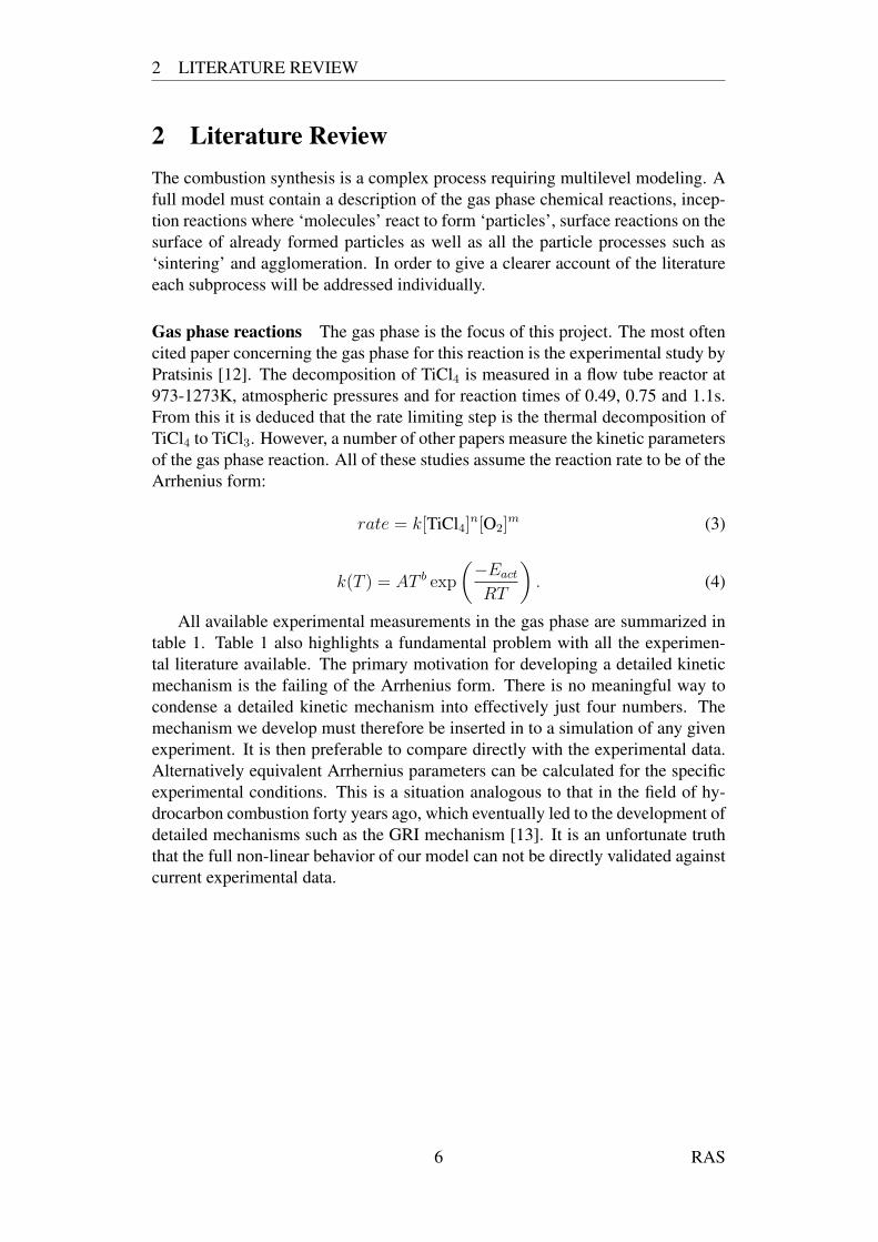
where a is the size of the box, m is the mass. This is inserted into equation 11,the summation can be written as the product of summation for each dimension.Assuming the energy levels are very close together this can be approximated byan integral:

qtrans (V, T ) =

(∫ ∞0

exp

(−π2~2n2

2kBTma2

)dn

)3

=

(mkBT

2π~2

) 32

V (21)

Electronic partition function The first excited electronic state is generally somuch higher in energy than the ground state that it makes a negligible contributionto the partition function and is sensibly ignored. The multiplicity of the groundstate is equivalent to the degeneracy and so the partition function is multiplied bythe multiplicity.

Relationship between partition function and thermodynamic potentials Themathematical relationships between H, S, Cp and G and the partition function qare presented in Equations 22 to 26.

S = NkB

[∂ (T ln q)

∂T− lnN + 1

](22)

Cv = NkBT∂2 (T ln q)

∂T 2(23)

Cp = Cv +NkB (24)

H (T )−H (0) =

∫ T

0

CpdT =NkBT

2

q

∂q

∂T+NkBT (25)

G = H − TS (26)

All the information required to calculate the partition function and thus (al-most) all the thermodynamic potentials is generated by the quantum calculations.The one quantity that can not currently be calculated ab initio is H(0). This mustbe known empirically or inferred using a reaction linking the species in questionto other species with known H(0).

Enthalpies of formation: Isodesmic and Isogyric Reactions The enthalpy offormation, ∆fH , is the enthalpy change associated with the formation of a chem-ical species in it’s standard state from the constituent elements in their standardstates. It is not currently possible for quantum chemistry software to calculate thisand it is necessary to connect a species to others with known ∆fH via a hypo-thetical reaction. The errors in the calculation of energy with quantum softwareare believed to be systematic and so should cancel out when calculating the en-thalpy change of a chemical reaction. There is however a complication. Thesesystematic errors are associated with particular bonds. The Ti-Cl bond will have

19 RAS

4 STATISTICAL MECHANICS

a different error to the Ti-O bond. There are two ways of dealing with this is-sue. The so called bond additivity correction (BAC) method sets out to calculatecorrections for every type of relevant bond. We however decided to implementthe more straightforward approach of carefully selecting the reactions used tocalculate ∆fH . Ideally a so-called isodesmic reaction may be found where bythe bonds broken in the reactants are the same as the bonds formed in the prod-ucts. The errors associated with each bond will then cancel out assuming themolecular environment of the bond is not important. If it is impossible to findan isodesmic reaction linking to known species then an isogyric reaction may befound where the number of electron pairs and unpaired electrons is the same on ei-ther side of the reaction. The standard enthalpy of formation of Ti2O2Cl6 was de-rived from the isogyric reaction Ti2O2Cl6 � 2 TiOCl2 + Cl2 and Ti2O2Cl5 fromTi2O2Cl5 + TiCl4 � 2 TiOCl2 + Cl2 + TiCl3. TiCl2OCl was derived from theanisogyric reaction TiCl2OCl � TiOCl2 + Cl so is expected to be the least ac-curately determined ∆fH298K .

Table 3: Calculated thermochemistry at 298 K.species ∆fH298 K S298 K rot. const. vibrational frequencies

kJ/mol J/mol K GHz cm−1

TiCl2OCl −475 396.9 1.9445, 0.9729, 0.6484 17.1, 44.8, 93.7, 131, 174,341, 474, 483, 950

Ti2O2Cl6 −1503 562.3 0.5965, 0.2506, 0.2497 17.9, 18.7, 36.3, 84.8, 93.6,101, 115, 135, 135, 137, 155,163, 206, 299, 324, 388, 404,455, 473, 487, 505, 509, 574,902

Ti2O2Cl5 −1272 537.5 0.7562, 0.2939, 0.2611 14.1, 28.3, 45.8, 79.5, 82.3,100, 118, 130, 140, 162, 194,318, 335, 366, 401, 473, 483,493, 501, 575, 885

4.1.1 NASA polynomials

The final aim is to produce a ChemKin and Cantera input for the overall reactionscheme. These are files that can be read in to software packages that model thebehavior of chemical systems. That is, model the time variation of all species con-centrations in time varying pressures and temperatures from some given startingconcentrations. The thermodynamic functions required have complicated temper-ature dependence and so to simplify the computation they are modeled by polyno-mial functions. The three functions needed are approximated with the followingpolynomials:

CpR

= a1 + a2T + a3T2 + a4T

3 + a5T4 (27)

H

R= a1T +

a2

2T 2 +

a3

3T 3 +

a4

4T 4 +

a5

5T 5 + a6 (28)

S

R= a1 lnT + a2T +

a3

2T 2 +

a4

3T 3 +

a5

4T 4 + a7 (29)

where Cp is the molar heat capacity at constant pressure, H is the standard en-thalpy of formation, S is the entropy, R is the ideal gas constant, and T is the

20 RAS

4 STATISTICAL MECHANICS

0

10

20

30

40

50

60

0 1000 2000 3000 4000Temperature (K)

Cp/

R

Figure 8: The heat capacity, Cp, calculated using RRHO (red line) and the polynomial fit(black line).

temperature in Kelvin.As you can see, due to the relationships between these functions the full tem-

perature behavior is fully described by only seven coefficients. The situation isslightly complicated by the fact that at high temperatures some of the higher en-ergy modes rapidly become occupied and there is a fairly clear elbow in for in-stance the heat capacity temperature dependence. For this reason a single polyno-mial can not give a very accurate fit and it is necessary to define two polynomialsthat when joined together must satisfy the conditions of continuity and smooth-ness. A python script was written to fit these two polynomials while enforcing theconstraints. This script was also used to optimize the temperature at which thetwo polynomials join in order to create the most accurate overall fit.

The python script was designed to read either the output files directly or thecalculated thermodynamic properties from a structured query language (SQL)database and print out both the required forms. Figure 9 shows examples in bothChemkin and Cantera form.

4.2 Transition state theoryFor a bimolecular reaction with a barrier, transition state theory (TST) predicts therate as:

k(T ) =kBT

2π~Q 6=

QAQB

exp

(−EactkBT

)(30)

where Q6= is the total partition function of the transition state, QA and QB thepartition function of the the reactants A and B and ∆Eact is the energy differencebetween the lowest energy level of the reactants and the transition state. Thetotal partition function is calculated as the product of the vibrational, translational,rotational and electronic partition functions.

The reaction rates were calculated using TST in the range 300 K to 3000 K

21 RAS

4 STATISTICAL MECHANICS

Cantera form:

# CH2OSi(OCH3)(OC2H3)OHspecies(name = " MYOMOVOSOL ", atoms = " C:4 H:9 O:4 Si:1 ", thermo = ( NASA( [ 25.0 , 829.35143236 ], [ 2.338789747E+000 ,9.037104748E-002 , -1.157698449E-004 , 1.045322476E-007 , -4.279297301E-011 , -1.139609569E+005 , 1.586287679E+001 ] ), NASA( [ 829.35143236 , 4000.0 ], [ 1.550372777E+001 ,3.767841478E-002 , -1.688788031E-005 , 3.586336822E-009 , -2.930899057E-013 , -1.169557189E+005 , -4.875186312E+001 ] ) ), note = " CH2OSi(OCH3)(OC2H3)OH MAY08 " )

Chemkin form:

! CH2OSi(OCH3)(OC2H3)OH MYOMOVOSOL MAY08 C 4H 9O 4Si 1G 25 4000 829.351 1+1.550373E+001 +3.767841E-002 -1.688788E-005 +3.586337E-009 -2.930899E-013 2-1.169557E+005 -4.875186E+001 +2.338790E+000 +9.037105E-002 -1.157698E-004 3+1.045322E-007 -4.279297E-011 -1.139610E+005 +1.586288E+001 4

Figure 9: Example ChemKin and Cantera files for the speciesCH2OSi(OCH3)(OC2H3)OH.

in 10 K steps and a linear least-square fitting algorithm was used to fit the ratecoefficients A, n and Eact applying the modified Arrhenius expression:

k(T ) = AT l exp

(−EactRT

)(31)

4.2.1 Variational transition state theory

Provided that a) no reaction trajectory goes through the transition state and thenreturns through it to the reactants and b) the reactants are maintained in a Boltz-mann distribution, then TST is exact, at least for a reaction following classicaldynamics [41]. These two conditions are not always met and since the TST esti-mate is an upper limit variational transition state theory was developed wherebythe transition state is varied until the minimum rate is found. In the absence of anenergy barrier TST can not be used since there is no obvious choice for the tran-sition state. Variational transition state theory (VTST) must be used. For a goodoverview of current a priori methods for calculating rate constants see Sumathiand Green (2002) [42]. VariFlex [43] is a program package for estimating rateconstants of several types of gas phase reactions. Variflex was used here to cal-culate the rate of reaction of R1 including pressure dependence and falloff usingVTST. It takes approximately two hours to run and as output gives the high andlow pressure limit rate constants at a range of temperatures and pressures speci-fied by the user. It is then necessary to fit the ‘Troe’ form to this rate constant.This was done by C. Franklin Goldsmith, a graduate student at MIT who wrote aMatlab script specifically for this purpose. It is anticipated that we will wish to domore of these VariFlex calculations and will be writing a Python script to do thiswith a standard least squares fit.

22 RAS

4 STATISTICAL MECHANICS

The Troe parameters The Lindemann falloff form is a crude non specific methodfor estimating the rate falloff at low pressures. This treatment applies in mostmodels if no specific falloff parameters are given. In this Lindemann scheme,at pressures intermediate to the high and low pressure limits, the rate constant isgiven by the Lindemann formula:

k =kinf

1 + kinf/k0[M ](32)

Where k is the rate constant, kinf is the high pressure limit rate constant, k0

is the low pressure limit rate constant and [M ] is the bath gas concentration. TheTroe parameters provide a more refined treatment of pressure effects than Linde-mann. The falloff parameter Fcent for a unimolecular reaction is calculated fromthe values of α, T ∗∗∗, T ∗, and T ∗∗ by the formula of Troe

Fcent = (1− α) exp(−T/T ∗∗∗) + α exp(−T/T ∗) + exp(−T ∗∗/T ) (33)

Where Fcent is the factor by which the rate constant of a given reaction attemperature T and reduced pressure Pr (given by equation 34) is less than thevalue kinf/2 which it would have if reactions behaved according to the Lindemannformula.

Pr = k0[M ]/kinf = 1.0 (34)

The four Troe parameters are the only inputs required by ChemKin and Can-tera to fully describe the pressure dependence with falloff. The broadening factor,which describes how sharp the join between the high and low pressure limits are,is calculated from Fcent. For a more detailed explanation of the Troe paramatersconsult the ChemKin manual [44].

23 RAS

5 SIMULATIONS

5 SimulationsOnce the changes were made to the model we then needed to find some exper-imental data to compare to. As stated in the literature review section the mostoften cited experimental study is Pratsinis et al. (1990) [12]. Pratsinis assumes ar-rhenius like behavior and reports the pre-exponential factor and activation energy.We therefore have to condense the complex non linear behavior of the model intojust two numbers. It is perfectly possible that the mechanism may behave well in agiven pressure-temperature regime but not in another. Favorable comparison withexperiments that typically take place at significantly lower temperatures and pres-sures and in the presence of a bath gas does not necessarily validate the model. Itshould be remembered that the central aim is to model an industrial reactor. Thethird year PhD student Richard West helped significantly with the simulations.Coupling to the population balance model in the plug flow reactor simulation wasconducted largely by him.

5.1 Rapid compression machineThe PhD thesis by Raghavan describes investigations of the kinetics of TiCl4 ox-idation using a rapid compression machine (RCM) [20]. A mixture of 0.3 mol%TiCl4 and 1 mol% O2 in Argon was loaded into a cylinder at reduced pressure, thenrapidly compressed causing temperature and pressure of the gas to rise quickly.The temperature was calculated from the pressure, volume, and starting tempera-ture, according to a hot-core model in which 20% of the volume (near the walls) iscompressed isothermally. The piston was designed to bounce, resulting in a shortpeak in temperature, found to be well approximated by a lorentzian. The reac-tion time reported was the half-width at half-maximum (HWHM) of a lorentzianfitted to the top 10% of the temperature profile. The concentration of TiCl4 wasmeasured before and after compression using fourier transform infrared (FTIR)spectroscopy.

−0.2

0

0.2

0.4

0.6

0.8

1

500Tp (K)

1−(N

/N0)

SimulationRaghavanPratsinis

1000 1500 2000

Figure 10: TiCl4 consumed (1-N/N0) verses max temperature in the rapid compressionmachine

24 RAS

5 SIMULATIONS

This RCM was simulated here with the new gas-phase kinetic model, usingCantera and Python. In our simulation, the piston was driven sinusoidally for onestroke, with a speed and compression ratio adjusted to ensure that a Lorentzianleast-squares fitted to the hottest 10% or our temperature profile had a Tp andHWHM equal to Raghavan’s reported values. This was repeated for the sixteencombinations of Tp and tc reported in [20]. The shape of the temperature profilefrom this sinusoidal compression is similar to the temperature profiles of the RCMgiven in [20]. The simulation was spatially homogeneous, so following the hot-core description in [20], the simulated conversion was scaled by 0.8 (20% of thegas remained unreacted). Because the gas is heated rapidly and for a short timethe walls do not heat up, so surface reactions were neglected.

5.2 Plug flow reactorThere is no analytic method to condense the complex mechanism into a one stepequivalent form. It is therefore necessary to insert the mechanism in to a simulatedpressure temperature regime, track the decomposition of some species and fit anarrhenius curve to this data. To simulate the comprehensive model of chemistryand particle dynamics, we use the extended surface-volume model with primaryparticle tracking described in [9, 5], coupled to the gas phase chemistry simula-tion using operator splitting [10]. This is used to model the tubular flow reactorused by Pratsinis [12] to measure the overall reaction kinetics. In [12], a flowof 0.2 mol% TiCl4 and 1 mol% O2 in Argon was fed to a 3.18 mm-I.D. tube, a∼30 cm section of which was heated to 973–1273 K in a furnace. The concentra-tion of TiCl4 leaving the flow tube (Co) was measured using FTIR spectroscopy.Assuming that the reaction rate is first order in [TiCl4] with Arrhenius kinetics(keff = A exp (−Eact/RT )) and that all reaction occurs during the time t that thegas spends in an isothermal zone at temperature T then

−(ln (Co/Ci)

)/t)

= keff = A exp(−Eact/RT ). (35)

A plot of ln(−(ln (Co/Ci)

)/t)

versus 1/T (Fig. 11) would thus give a straightline from which the apparent activation energy Eact and pre-exponential constantA can be determined. This is the analysis performed in [12], and our simulationresults are processed the same way for easy comparison. The assumption of con-stant T for a time t was only made for the analysis: the simulations covered theentire temperature profile (given in [12]) and included thermal expansion of thegas as the temperature varied.

The simulations using our new gas-phase kinetic model (Fig. 11, solid lines)consume much less TiCl4 than the observations reported in [12]. At 1133 K thekeff fitted to the simulation is between 14 and 45 times lower (slower rate) thanthat fitted to the experiment, depending on which residence time is simulated. Theapparent activation energy is higher in the simulation, so at 993 K the discrepancyincreases to kexpt

eff /ksimeff = 5.2× 103.

The simulations were repeated allowing for deposition and reaction of TiCl4on the inside surface of the tube, using the expression for surface growth of a TiO2

film given by Ghoshtagore [45] (Eqn. 5).

25 RAS

5 SIMULATIONS

-10

-8

-6

-4

-2

0

2

4

0.85 0.9 0.95 1

103/T(K)

ln(k

eff)

0.49 s0.75 s1.1 s

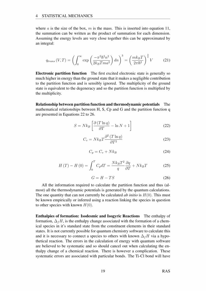
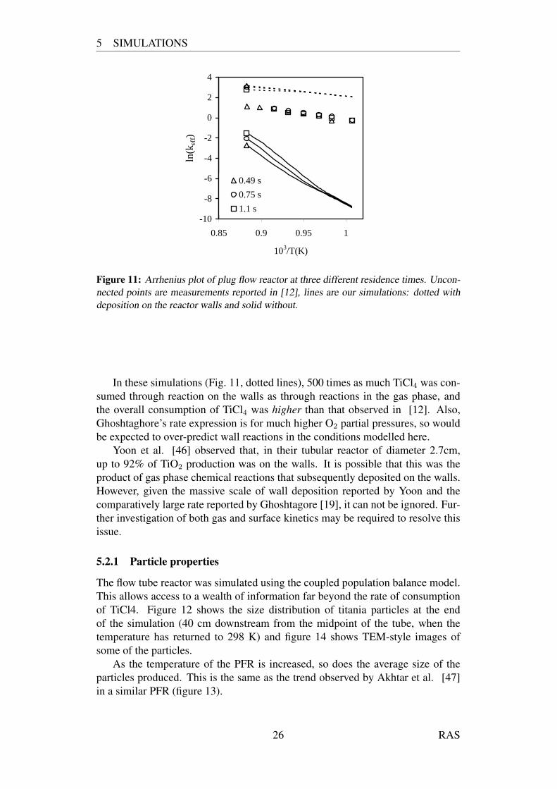
Figure 11: Arrhenius plot of plug flow reactor at three different residence times. Uncon-nected points are measurements reported in [12], lines are our simulations: dotted withdeposition on the reactor walls and solid without.

In these simulations (Fig. 11, dotted lines), 500 times as much TiCl4 was con-sumed through reaction on the walls as through reactions in the gas phase, andthe overall consumption of TiCl4 was higher than that observed in [12]. Also,Ghoshtaghore’s rate expression is for much higher O2 partial pressures, so wouldbe expected to over-predict wall reactions in the conditions modelled here.

Yoon et al. [46] observed that, in their tubular reactor of diameter 2.7cm,up to 92% of TiO2 production was on the walls. It is possible that this was theproduct of gas phase chemical reactions that subsequently deposited on the walls.However, given the massive scale of wall deposition reported by Yoon and thecomparatively large rate reported by Ghoshtagore [19], it can not be ignored. Fur-ther investigation of both gas and surface kinetics may be required to resolve thisissue.

5.2.1 Particle properties

The flow tube reactor was simulated using the coupled population balance model.This allows access to a wealth of information far beyond the rate of consumptionof TiCl4. Figure 12 shows the size distribution of titania particles at the endof the simulation (40 cm downstream from the midpoint of the tube, when thetemperature has returned to 298 K) and figure 14 shows TEM-style images ofsome of the particles.

As the temperature of the PFR is increased, so does the average size of theparticles produced. This is the same as the trend observed by Akhtar et al. [47]in a similar PFR (figure 13).

26 RAS

5 SIMULATIONS

0.01

0.1

1

10

100

0.0001Dp (µm)

dP/d

log

Dp

T=993 K

T=1073 KT=1133 K

T=1293 K

0.001 0.01 0.1 1

Figure 12: Particle size distributions from the PFR simulation with residence time in thehot-zone of 0.49 s.

Figure 13: Particle size distributions from Akhtar et al (1991)

Figure 14: Simulated TEM Images from the exit of the PFR simulation with residencetime in the hot-zone of 0.49 s and furnace temperatures 993, 1017, 1073 and 1293 K (leftto right).

27 RAS

6 CONCLUSIONS

6 ConclusionsThe results found using quantum chemistry have led to an improved kinetic mech-anism for the combustion synthesis of titanium dioxide nanoparticles. This newmechanism has been implemented in to two simulations allowing comparison withexperiments from the literature for the first time. The mechanism compares wellwith the RCM experiment of Raghavan [20] but less so with the flow tube exper-iment of Pratsinis. This led us to the hypothesis that Pratsinis may be measuringthe surface reactions to some extent. This is an important new result as the workis cited by many other papers. It is of greater importance still because the PFRis a standard experimental setup used in many other fields. Adding the surfacegrowth rate of Ghoshtagore [19] led to the overestimation of the rate comparedto Pratsinis [12]. This discrepancy remains unexplained. It may be because oursimulation fails to take mass transfer into account. It could also be because theGhoshtagore rate is simply too high, it is only calculated at temperatures of up to1023 K but our simulations go up to 1293 K. Extrapolation to this degree is notrecommended

The major findings after one year of research are:

• Three new species are presented in figure 5.

• One new pressure dependent reaction rate constant is estimated.

• 15 new reactions are added to the mechanism inherited from West [5].

• The new kinetic model is used to simulate two experiments from the litera-ture.

• Rates for a new PAH mechanism are calculated with the help of the firstyear PhD student Markus Sander.

• The results from quantum jobs on SiaCbOcHd species done by anothermember of the group are converted into thermochemistry in ChemKin andCantera form enabling them to be used in a full kinetic model.

These results represent a significant effort and demonstrate real progress. Thework done this year has provided a solid grounding in the field and has left definiteideas about the best way to move forward, which will be discussed in the nextchapter.

28 RAS

7 FUTURE WORK

7 Future WorkLet us begin with a statement of purpose. The two major research aims are:

• Find the critical nucleus and improve the coupling between the gas phaseand particle population balance.

• Add AlCl3 and other chemicals to the mechanism and understand their ef-fect on the end product.

These are highly non trivial problems. The big difficulty attached to both is com-plexity. A back of the envelope calculation to estimate the number of possiblemolecules containing x titanium atoms reveals the enormity of the task. It is sim-ply not possible to manually find all the species and reactions involved in thegas phase. There are two ways to deal with this fundamental difficulty: a) limitourselves to ‘important’ species and reactions. It may be possible to find somebroadly applicable rules for the species and reactions that will contribute signifi-cantly to the rate. b) Automate the process. If we desire a gas phase mechanismincluding molecules up to the critical nucleus then we must automatically searchthrough possible species. Fortunately there is already a methodology for doingexactly this. The PhD thesis of Song [48] presents a ‘Reaction Mechanism Gener-ator’ (RMG) for hydrocarbon chemistry. It is a long term aim to get this workingfor the combustion of TiCl4. This is a task scratched upon in Richard West’s PhDthesis [49].

7.1 Short termIn the coming months work will continue on the effect of aluminium on thebandgap and other properties of both rutile and anatase. This is the next publica-tion to work towards and I will be presenting it as a work in progress poster at TheInternational Combustion Symposium in August. It may also lead to insight in tothe effect of aluminium on particle inception and the reason that it preferences ru-tile given that it is known to reduce the stability of both phases. One suggestion isthat it prevents crystallization until the particle is larger. Since anatase is actuallythe more stable phase for very small particles this might lead to more rutile. Ithas also been suggested that it reduces the temperature at which anatase can un-dergo a phase transformation but the physical reason for this is not known. Oncethe modus operandi is established it then should be possible to conduct a detailedstudy into the effects of other dopants. There is significant interest into nitrogenand boron doping for the application of TiO2 in not just DSSCs but also as a pho-tocatalyst where the band gap again critically effects the wavelength dependence.These jobs will be executed largely on the high performance clusters ‘DARWIN’(in Cambridge) and ‘HELICS’ (in Heidelberg). This work is extremely computa-tionally intensive and can not be done on the CoMo group cluster. The long timesof these jobs (1+ days) does mean that other work may be done concurrently. Wewill learn how to use the reaction mechanism generator RMG. This will involveprogramming with the object oriented programming package Java and will be thetopic of a Part IIB research project that I will be supervising next year. The stu-dent and I will make adjustments to RMG to allow the consideration of titanium

29 RAS

7 FUTURE WORK

oxygen chorine systems. Hopefully it will be possible for the student to producea rough copy of the current detailed mechanism by the end of the year.

7.2 Medium termWithin a year RMG should have been extended to the titanium-oxygen-chlorinesystem and be able to replicate the Kinetic model of West [6, 5] to some extent.It may even be possible to automate the quantum calculations. In order to do thiswe must develop an algorithm for guessing geometries and write a program togenerate the appropriate input files required by the quantum software. By this timethe first year PhD student Markus Sander and I should have developed a full suiteof Python tools to calculate the thermochemistry from the quantum jobs. It couldthen be possible to couple this to the RMG allowing fully automated generationof not just the mechanism but also the rates and equilibrium concentrations.

The work that has been done with python is part of a bigger overall scheme.it represents a step towards a unified set of tools that takes a quantum job as inputand outputs the thermochemistry automatically. Together with the first year PhDstudent Markus Sander there should be a full framework to automatically selectisodesmic/isogyric reactions from a database of known species and provide theCantera and Chemkin polynomials within a year. This will include the polynomialfitting script already written.

I hope that within a year there should be a much better understanding of thecritical nucleus. A simple algorithm is being developed for finding paths fromsmall molecules to both of the crystal forms (ignoring chlorine). Very crudelyit will involve starting with a large molecule made up of a number of primitivecells and removing TiO2 monomers until we are left with just one monomer or theopposite, starting with TiO” and building up to something approaching the crystalphase.

TiO2 → Ti2O4 → Ti3O6 → Ti4O8 → etc.→ Rutile or anatase

We could then plot energy per monomer as a function of monomer number andfind the critical nucleus. One problem is that any mechanism would certainlyinvolve reactions that didn’t conserve a Ti:O ratio of 1:2 such that it would be im-possible to plot energy per monomer. Although only a minute number of possiblepaths could be charted manually like this it might give some measure of how bigour gas phase mechanism needs to be. It may then be possible to estimate thenumber of possible paths and generate an estimate for particle inception.

7.3 Full multilevel modelling including aluminiumOnce RMG is at the stage where it can reproduce the ‘handmade’ mechanism ofWest. It will then be used to extend the gas phase mechanism to include alu-minium and describe molecules up to the critical nucleus. Depending on the sizeof the critical nucleus this may be unfeasible. Even if it is possible to automati-cally generate the species and reactions, each species must still be optimized usingquantum chemistry in order to have a thermodynamically consistent model. If thecritical nucleus were say 100 monomers it would simply not be possible to inves-

30 RAS

7 FUTURE WORK

tigate all of the millions of possible species let alone the reactions between them.The particle inception events currently used to couple the gas phase with our par-ticle population balance models represent the biggest flaw in the overall model.This is where we should concentrate our efforts. The critical nucleus is a logicalchoice for the maximum-molecule/smallest-particle considered because it is thesize after which particles are more likely to grow than shrink. However, we needto find out more before we can verify the sensibility of this method.

While a large amount of effort will be expended on improving the mechanismwe must remember that even if we knew the true mechanism it would be of lit-tle use without the rates of the intermediate reaction. It is there for a long termtask to calculate rates for more of the early reactions. This is a slow and, to befrank, tedious task but it is necessary if the kinetic model is to be vigorous. I havementioned the possibility of automating this task and we will look into that but itis imperative that throughout the next two years we steadily calculate some morerate constants. Remember, the majority of intermediate reactions still proceed atthe collision limited rate in our model. One important thing to understand hereis that because all these rates are currently overestimated does not mean that themodel will necessarily overestimate. The system is highly non linear. At onepoint we accidentally used the old model in the RCM simulation with the rate R1effectively much faster than it currently is. This actually led to reduction in the theoverall rate. The fact that our model underestimates rate could actually be solvedby calculating the intermediate rates thus slowing them down. Another long termaim is have a better understanding of the non-linear behavior of the model includ-ing pressure dependence. This, after all, is the motivation for a detailed kineticmodel instead of using a basic arrhenius form.

I have described a number of possible avenues for progress and am confidentthat there will be enough results within the first three years and certainly withinfour to produce a high quality PhD thesis.

31 RAS

REFERENCES

References[1] J. Emsley, Molecules at an Exhibition, Oxford University Press, 1999.

[2] U. Diebold, The surface science of titanium dioxide, Surf. Sci. Rep. 48 (5-8)(2003) 53–229.

[3] B. Karlemo, P. Koukkari, J. Paloniemi, Formation of gaseous intermediatesin titanium(IV) chloride plasma oxidation, Plasma Chem. Plasma Process.16 (1996) 59–77.

[4] M. Steveson, T. Bredow, A. R. Gerson, MSINDO quantum chemical mod-elling study of the structure of aluminium-doped anatase and rutile titaniumdioxide, Phys. Chem. Chem. Phys. 4 (2) (2002) 358–365.

[5] R. H. West, M. S. Celnik, O. R. Inderwildi, M. Kraft, G. J. O. Beran, W. H.Green, Toward a comprehensive model of the synthesis of TiO2 particlesfrom TiCl4, Ind. Eng. Chem. Res. 46 (19) (2007) 6147–6156.

[6] R. H. West, G. J. O. Beran, W. H. Green, M. Kraft, First-principles thermo-chemistry for the production of TiO2 from TiCl4, J. Phys. Chem. A 111 (18)(2007) 3560–3565.

[7] R. H. West, R. A. Shirley, M. Kraft, C. F. Goldsmith, W. H. Green, A detailedkinetic model for combustion synthesis of titania from TiCl4, in: Proceed-ings of the Combustion Institute, submitted 2008.

[8] R. Patterson, J. Singh, M. Balthasar, M. Kraft, J. R. Norris, The linear pro-cess deferment algorithm: A new technique for solving population balanceequations, SIAM J. Sci. Comput. 28 (1) (2006) 303–320.

[9] R. I. A. Patterson, M. Kraft, Models for the aggregate structure of soot par-ticles, Combust. Flame 151 (2007) 160–172.

[10] M. Celnik, R. Patterson, M. Kraft, W. Wagner, Coupling a stochastic sootpopulation balance to gas-phase chemistry using operator splitting, Com-bust. Flame 148 (3) (2007) 158–176.

[11] S. Ln, A. Orlov, R. Berg, F. Garcia, S. Pedrosa-Jimenez, M. S. Tikhov, D. S.Wright, R. M. Lambert, Effective Visible Light-Activated B-Doped andB,N-Codoped TiO2 Photocatalysts, J. Am. Chem. Soc. 129 (2007) 13790–13791.

[12] S. E. Pratsinis, H. Bai, P. Biswas, M. Frenklach, S. V. R. Mastrangelo, Kinet-ics of titanium(IV) chloride oxidation, J. Am. Ceram. Soc. 73 (1990) 2158–2162.

[13] G. P. Smith, D. M. Golden, M. Frenklach, N. W. Moriarty, B. Eiteneer,M. Goldenberg, C. T. Bowman, R. K. Hanson, S. Song, W. C. Gardiner,V. V. Lissianski, Z. Qin, GRI-Mech 3.0, software package (2008).URL http://me.berkeley.edu/gri-mech/

32 RAS

REFERENCES

[14] Y. Suyama, K. Ito, A. Kato, Mechanism of Rutile Formation in Vapor PhaseOxidation of TiCl4 by Oxygen, J. inorg. nucl. Chem. (1974) 1883–1888.

[15] I. V. Antipov, B. G. Koshunov, L. M. Gofman, Kinetics of the reation oftitanium tetrachloride with oxygen, J. Appl. Chem. USSR (1967) 11–15.

[16] I. Mahawili, F. J. Weinberg, Ta study of titanium tetrachloride oxidation in arotating arc plasma jet, AIChE Symposium 75 (1979) 11–24.

[17] S. Toyama, M. Nakamura, H. Mori, K. Kanai, T. Nachi, The Production ofUltrafine Particles by Vapor Phase Oxidation from Chloride, Proc. 2nd Wld.Con. Part. Tech. (1990) 360–367.

[18] A. Kobata, K. Kusakabe, S. Morooka, Growth and transformation of TiO2

crystallites in aerosol reactor, AIChE J. 37 (3) (1991) 347–359.

[19] W. Ghoshtagore, A. J. Noreika, Growth characteristics of rutile film bychemical vapor deposition, J. Electrochem. Soc. 117 (1970) 1310–1314.

[20] R. Raghavan, Measurement of the high-temperature kineticsof titanium tetrachloride (TiCl4) reactions in a rapid compres-sion machine, Ph.D. thesis, Case Western Reserve University,http://www.case.edu/cse/eche/people/students/theses/RaghavanRam-PhD.pdf (August 2001).

[21] R. D. Smith, R. A. Bennett, M. Bowker, Measurement of the surface-growthkinetics of reduced TiO2(110) during reoxidation using time-resolved scan-ning tunneling microscopy, Phys. Rev. B: Condens. Matter Mater. Phys.66 (3) (2002) 035409.

[22] O. Inderwildi, M. Kraft, Adsorption, Diffusion and Desorption of Chlo-rine on and from Rutile TiO2{110}: A Theoretical Investigation.,ChemPhysChem 8 (2007) 444–451.

[23] S. E. Pratsinis, P. T. Spicer, Competition between gas phase and surfaceoxidation of TiCl4 during synthesis of TiO2 particles, Chem. Eng. Sci. 53(1998) 1861–1868.

[24] P. T. Spicer, O. Chaoul, S. Tsantilis, S. E. Pratsinis, Titania formation byTiCl4 gas phase oxidation, surface growth and coagulation, J. Aerosol Sci.33 (2002) 17–34.

[25] S. Tsantilis, S. E. Pratsinis, Narrowing the size distribution of aerosol-madetitania by surface growth and coagulation, J. Aerosol. Sci. 35 (2004) 405–420.

[26] N. M. Morgan, C. G. Wells, M. J. Goodson, M. Kraft, W. Wagner, A new nu-merical approach for the simulation of the growth of inorganic nanoparticles,J. Comput. Phys. 211 (2) (2006) 638–658.

[27] Y. Xiong, S. E. Pratsinis, Formation of agglomerate particles by coagulationand sintering–part i. A two-dimensional solution of the population balanceequation, J. Aerosol Sci. 24 (3) (1993) 283–300.

33 RAS

REFERENCES

[28] J. Singh, R. I. A. Patterson, M. Balthasar, M. Kraft, W. Wagner, Modellingsoot particle size distribution: Dynamics of pressure regimes, Technical Re-port 25, c4e-Preprint Series, Cambridge (2004).

[29] B. O’Regan, M. Gratzel, A low-cost, high-efficiency solar cell based on dye-sensitized colloidal TiO2 films, Nature 335 (1991) 737.

[30] M. Gratzel, Dye-sensitized solar cells, J. Photochem. Photobio. C 4 (2003)145–153.

[31] P. Atkins, Molecular Quantum Mechanics, Oxford University Press, 1997.

[32] P. Hohenberg, W. Kohn, Inhomogeneous electron gas, Phys. Rev. B (1964)864–871.

[33] F. A. Hamprecht, A. J. Cohen, D. J. Tozer, N. C. Handy, Development and as-sessment of new exchange-correlation functionals, J. Chem. Phys. 109 (15)(1998) 6264–6271.

[34] A. Boese, N. Handy, A new parametrization of exchange–correlation gener-alized gradient approximation functionals, J. Chem. Phys. 114 (13) (2001)5497–5503.

[35] M. J. Frisch, G. W. Trucks, H. B. Schlegel, G. E. Scuseria, M. A. Robb, J. R.Cheeseman, J. A. Montgomery, Jr., T. Vreven, K. N. Kudin, J. C. Burant,J. M. Millam, S. S. Iyengar, J. Tomasi, V. Barone, B. Mennucci, M. Cossi,G. Scalmani, N. Rega, G. A. Petersson, H. Nakatsuji, M. Hada, M. Ehara,K. Toyota, R. Fukuda, J. Hasegawa, M. Ishida, T. Nakajima, Y. Honda,O. Kitao, H. Nakai, M. Klene, X. Li, J. E. Knox, H. P. Hratchian, J. B.Cross, V. Bakken, C. Adamo, J. Jaramillo, R. Gomperts, R. E. Stratmann,O. Yazyev, A. J. Austin, R. Cammi, C. Pomelli, J. W. Ochterski, P. Y. Ayala,K. Morokuma, G. A. Voth, P. Salvador, J. J. Dannenberg, V. G. Zakrzewski,S. Dapprich, A. D. Daniels, M. C. Strain, O. Farkas, D. K. Malick, A. D.Rabuck, K. Raghavachari, J. B. Foresman, J. V. Ortiz, Q. Cui, A. G. Baboul,S. Clifford, J. Cioslowski, B. B. Stefanov, G. Liu, A. Liashenko, P. Piskorz,I. Komaromi, R. L. Martin, D. J. Fox, T. Keith, M. A. Al-Laham, C. Y. Peng,A. Nanayakkara, M. Challacombe, P. M. W. Gill, B. Johnson, W. Chen,M. W. Wong, C. Gonzalez, J. A. Pople, Gaussian 03, Revision C.02, Gaus-sian, Inc., Wallingford, CT, 2004 (2003).

[36] A. D. Becke, Density-functional thermochemistry. III. The role of exact ex-change, J. Chem. Phys. 98 (7) (1993) 5648–5651.

[37] S. Clark, M. Segall, C. Pickard, P. Hasnip, M. Probert, K. Refson, M. Payne,First principles methods using CASTEP, Z. Kristallogr. 220 (2005) 567–570.

[38] J. P. Perdew, J. A. Chevary, S. H. Vosko, K. A. Jackson, M. R. Pederson, D. J.Singh, C. Fiolhais, Atoms, molecules, solids, and surfaces: Applications ofthe generalized gradient approximation for exchange and correlation, Phys.Rev. B: Condens. Matter Mater. Phys. 46 (11) (1992) 6671–6687.

34 RAS

REFERENCES

[39] W. DeMore, S. Sander, D. Golden, R. Hampson, M. Kurylo, C. Howard,A. Ravishankara, C. Kolb, M. Molina, Chemical kinetics and photochemicaldata for use in stratospheric modeling, Evaluation Number 15, Tech. Rep.JPL 06-2, NASA Jet Propulsion Laboratory, Jet Propulsion Laboratory, 4800Oak Grove Drive, Pasadena, California 91109-8099 USA (1997).

[40] NIST, Chemical Kinetics Database on the Web. Standard ReferenceDatabase 17, version 7.0 (web version), release 1.4 (November 2007).URL http://kinetics.nist.gov/

[41] M. J. Pilling, P. W. Seakins, Reaction Kinetics, Oxford University Press,Great Clarendon Street, Oxford, OX2 6DP, 1995.

[42] R. Sumathi, W. Green, A priori rate constants for kinetic modeling, Theor.Chem. Acc. 108 (4) (2002) 187–213.

[43] S. J. Klippenstein, A. F. Wagner, R. C. Dunbar, D. M. Wardlaw, S. H. Robert-son, J. A. Miller, VariFlex, software package (2002).URL http://chemistry.anl.gov/chem-dyn/VariFlex/

[44] R. J. Kee, F. M. Rupley, J. A. Miller, Chemkin-II: A fortran chemical ki-netics package for the analysis of gas-phase chemical kinetics, Tech. Rep.SAND89-8009, Sandia National Laboratories (1989).

[45] R. N. Ghoshtagore, Mechanism of heterogeneous deposition of thin film ru-tile, J. Electrochem. Soc. 117 (1970) 529–534.

[46] J. D. Yoon, K. Y. Park, H. D. Jang, Comparison of titania particles betweenoxidation of titanium tetrachloride and thermal decomposition of titaniumtetraisopropoxide, Aerosol Sci. Technol. 37 (8) (2003) 621–627.

[47] M. K. Akhtar, Y. Xiong, S. E. Pratsinis, Vapor synthesis of titania powder bytitanium tetrachloride oxidation, AIChE J. 37 (10) (1991) 1561–1570.

[48] J. Song, Building robust chemical reaction mechanisms: Next generation ofautomatic model construction software, Ph.D. thesis, Massachusetts Instituteof Technology, Camridge MA, USA (February 2004).URL http://hdl.handle.net/1721.1/30058

[49] R. West, Modelling the chloride process for titanium dioxide synthesis,Ph.D. thesis, Cambridge University, Camridge , UK (May 2008).

35 RAS

8 NOMENCLATURE

8 NomenclatureSymbol Meaningr Rate of reactionpTiCl4 Partial pressure of TiCl4A Pre-exponential factorEact Activation energykB Boltzmann constantT Temperature (in Kelvin)n Order of reaction with respect to TiCl4m Order of overall reaction with respect to O2

R Ideal gas constantCp Molar heat capacity at constant pressureH Standard enthalpy of formationS Standard entropy of formationH Molecular Hamiltonian operatorE Energy of the molecule (eigenvalue of H)Helec Hamiltonian of the electrons onlyT Kinetic energy operatorVNe Electron-nucleus attractionHee Pairwise repulsion of electronsψ Wavefunctionxi Position of electron iRi Position of nucleus iN Number of electronsn Vibrational quantum numberN Number of independent, indistinguishable moleculesa Length of boxV Volume of boxm Molecule mass~ Planck’s constant divided by 2π∆H Change in Enthalpy∆S Change in Entropy∆G Change in Gibbs Free Energyωj Angular frequency associated of the jth normal modegi Degeneracy of state iεi Energy of the ith state

36 RAS

8 NOMENCLATURE

Acryonym DescriptionDFT Density Functional TheoryPSD Particle Size DistributionTST Transition State TheoryVTST Variational Transition State TheoryRRKM Rice-Ramsberger-Kassel-Marcus (theory)SCF Self-Consistent FieldHF Hartree-FockGAMESS General Atomic and Molecular Electronic Structure SystemCASTEP CAmbridge Serial Total Energy PackageGUI Graphical User InterfaceUFF Universal Force FieldRHF Restricted Hartree-FockPFR Plug Flow ReactorPSR Perfectly Stirred ReactorCSR Continuously Stirred ReactorRRHO Rigid-Rotator/Harmonic-OscillatorLDA Local Density ApproximationGGA Generalized Gradient ApproximationPAH Poly-Aromatic HydrocarbonSQL Structured Query LanguageFTIR Fourier Transform InfraRedHWHM Half-Width at Half-Maximum

37 RAS