Department of Business Administration FALL 2007-08 Demand Forecasting Demand Forecasting by Asst....
83
Department of Business Administration FALL 2007-08 Demand Forecasting Demand Forecasting by Asst. Prof. Sami Fethi
-
Upload
theodora-wiggins -
Category
Documents
-
view
220 -
download
7
Transcript of Department of Business Administration FALL 2007-08 Demand Forecasting Demand Forecasting by Asst....
Department of Business Administration
FALL 2007-08
Demand ForecastingDemand Forecasting
by
Asst. Prof. Sami Fethi
2
Managerial Economics © 2007/08, Sami Fethi, EMU, All Right Reserved.
Ch 5 : Demand Forecasting
What is meant by Forecasting and Why?What is meant by Forecasting and Why?
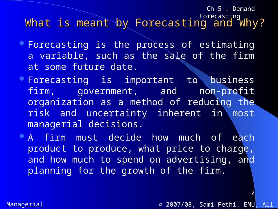
Forecasting is the process of estimating a variable, such as the sale of the firm at some future date.
Forecasting is important to business firm, government, and non-profit organization as a method of reducing the risk and uncertainty inherent in most managerial decisions.
A firm must decide how much of each product to produce, what price to charge, and how much to spend on advertising, and planning for the growth of the firm.

3
Managerial Economics © 2007/08, Sami Fethi, EMU, All Right Reserved.
Ch 5 : Demand Forecasting
The aim of forecastingThe aim of forecasting
The aim of forecasting is to reduce the risk or uncertainty that the firm faces in its short-term operational decision making and in planning for its long term growth.
Forecasting the demand and sales of the firm’s product usually begins with macroeconomic forecast of general level of economic activity for the economy as a whole or GNP.

4
Managerial Economics © 2007/08, Sami Fethi, EMU, All Right Reserved.
Ch 5 : Demand Forecasting
The aim of forecastingThe aim of forecasting
The firm uses the macro-forecasts of general economic activity as inputs for their micro-forecasts of the industry’s and firm’s demand and sales.
The firm’s demand and sales are usually forecasted on the basis of its historical market share and its planned marketing strategy (i.e., forecasting by product line and region).
The firm uses long-term forecasts for the economy and the industry to forecast expenditure on plant and equipment to meet its long-term growth plan and strategy.
5
Managerial Economics © 2007/08, Sami Fethi, EMU, All Right Reserved.
Ch 5 : Demand Forecasting
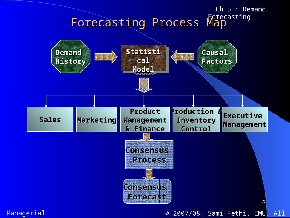
Forecasting Process MapForecasting Process Map
MarketingMarketingSalesSalesProductProduct
Management Management & Finance& Finance
Executive Executive ManagementManagement
Production &Production & Inventory Inventory
ControlControl
Causal Causal FactorsFactors
Statistical Statistical ModelModel
Statistical Statistical ModelModel
Demand Demand HistoryHistory
Consensus Consensus ProcessProcess
Consensus Consensus ForecastForecast
6
Managerial Economics © 2007/08, Sami Fethi, EMU, All Right Reserved.
Ch 5 : Demand Forecasting
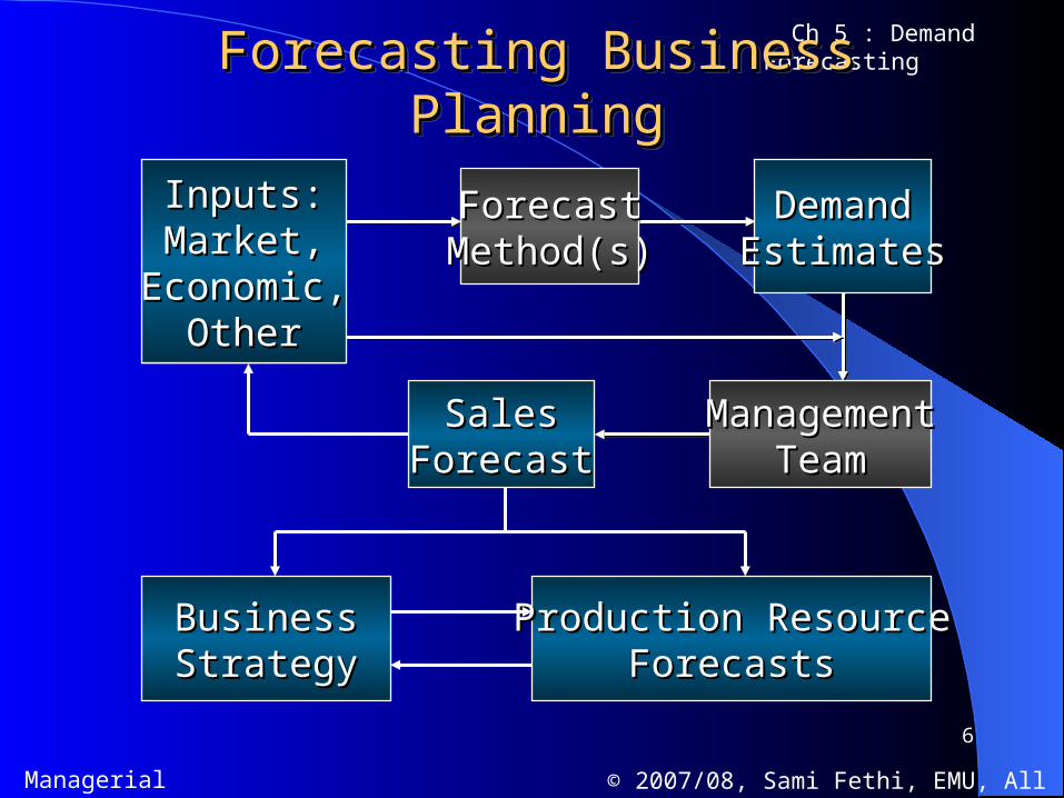
Forecasting Business PlanningForecasting Business PlanningForecasting Business PlanningForecasting Business Planning
ForecastForecastMethod(s)Method(s)
DemandDemandEstimatesEstimates
SalesSalesForecastForecast
ManagementManagementTeamTeam
Inputs:Inputs:Market,Market,
Economic,Economic,OtherOther
BusinessBusinessStrategyStrategy
Production ResourceProduction ResourceForecastsForecasts
7
Managerial Economics © 2007/08, Sami Fethi, EMU, All Right Reserved.
Ch 5 : Demand Forecasting
Forecasting TechniquesForecasting Techniques
A wide variety of forecasting methods are available to management. These range from the most naïve methods that require little effort to highly complex approaches that are very costly in terms of time and effort such as econometric systems of simultaneous equations.
Mainly these techniques can break down into two parts: qualitative approaches and quantitative approaches.

8
Managerial Economics © 2007/08, Sami Fethi, EMU, All Right Reserved.
Ch 5 : Demand Forecasting Qualitative approaches Qualitative approaches
&& Quantitative approaches Quantitative approaches
9
Managerial Economics © 2007/08, Sami Fethi, EMU, All Right Reserved.
Ch 5 : Demand Forecasting
Qualitative ForecastsQualitative Forecasts
Survey Techniques
Some of the best-know surveys– Planned Plant and Equipment Spending– Expected Sales and Inventory Changes– Consumers’ Expenditure Plans
Opinion Polls– Business Executives– Sales Force– Consumer Intentions

10
Managerial Economics © 2007/08, Sami Fethi, EMU, All Right Reserved.
Ch 5 : Demand Forecasting
What are qualitative forecast ?What are qualitative forecast ?
Qualitative forecast estimate variables at some future date using the results of surveys and opinion polls of business and consumer spending intentions.
The rational is that many economic decisions are made well in advance of actual expenditures.
For example, businesses usually plan to add to plant and equipment long before expenditures are actually incurred.

11
Managerial Economics © 2007/08, Sami Fethi, EMU, All Right Reserved.
Ch 5 : Demand Forecasting Qualitative ForecastsQualitative Forecasts
Surveys and opinion pools are often used to make short-term forecasts when quantitative data are not available
Usually based on judgments about causal factors that underlie the demand of particular products or services
Do not require a demand history for the product or service, therefore are useful for new products/services
Approaches vary in sophistication from scientifically conducted surveys to intuitive hunches about future events
The approach/method that is appropriate depends on a product’s life cycle stage
12
Managerial Economics © 2007/08, Sami Fethi, EMU, All Right Reserved.
Ch 5 : Demand Forecasting Qualitative ForecastsQualitative Forecasts
Polls can also be very useful in supplementing quantitative forecasts, anticipating changes in consumer tastes or business expectations about future economic conditions, and forecasting the demand for a new product.
Firms conduct opinion polls for economic activities based on the results of published surveys of expenditure plans of businesses, consumers and governments.
13
Managerial Economics © 2007/08, Sami Fethi, EMU, All Right Reserved.
Ch 5 : Demand Forecasting
Qualitative Forecasts TechniquesQualitative Forecasts Techniques
Survey Techniques– The rationale for forecasting based on surveys of economic intentions is that many economic decisions are made in advance of actual expenditures (Ex: Consumer’s decisions to purchase houses, automobiles, TV sets, furniture, vocation, education etc. are made months or years in advance of actual purchases)

14
Managerial Economics © 2007/08, Sami Fethi, EMU, All Right Reserved.
Ch 5 : Demand Forecasting
Qualitative Forecasts TechniquesQualitative Forecasts Techniques
Opinion Polls– The firm’s sales are strongly dependent on the level of economic activity and sales for the industry as a whole, but also on the policies adopted by the firm. The firm can forecast its sales by pooling experts within and outside the firm.
15
Managerial Economics © 2007/08, Sami Fethi, EMU, All Right Reserved.
Ch 5 : Demand Forecasting Opinion PollsOpinion Polls
Executive Polling- Firm can poll its top management from its sales, production, finance for the firm during the next quarter or year.
Bandwagon effect (opinions of some experts might be overshadowed by some dominant personality in their midst).
Delphi Method – experts are polled separately, and then feedback is provided without identifying the expert responsible for a particular opinion.
16
Managerial Economics © 2007/08, Sami Fethi, EMU, All Right Reserved.
Ch 5 : Demand Forecasting
Opinion PollsOpinion Polls
Consumers intentions polling- Firms selling automobiles, furniture, etc. can pool a sample of potential buyers on their purchasing intentions. By using results of the poll a firm can forecast its sales for different levels of consumer’s future income.
17
Managerial Economics © 2007/08, Sami Fethi, EMU, All Right Reserved.
Ch 5 : Demand Forecasting
Opinion PollsOpinion Polls
Sales force polling – Forecast of the firm’s sales in each region and for each product line, it is based on the opinion of the firm’s sales force in the field (people working closer to the market and their opinion about future sales can provide essential information to top management).
18
Managerial Economics © 2007/08, Sami Fethi, EMU, All Right Reserved.
Ch 5 : Demand Forecasting
Quantitative Forecasting ApproachesQuantitative Forecasting Approaches
Based on the assumption that the “forces” that generated the past demand will generate the future demand, i.e., history will tend to repeat itself.
Analysis of the past demand pattern provides a good basis for forecasting future demand.
Majority of quantitative approaches fall in the category of time series analysis.

19
Managerial Economics © 2007/08, Sami Fethi, EMU, All Right Reserved.
Ch 5 : Demand Forecasting
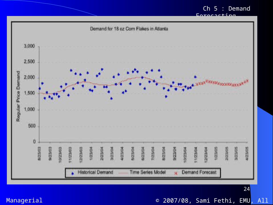
Time Series AnalysisTime Series Analysis
A time series (naive forecasting) is a set of numbers where the order or sequence of the numbers is important, i.e., historical demand
Attempts to forecasts future values of the time series by examining past observations of the data only. The assumption is that the time series will continue to move as in the past
Analysis of the time series identifies patterns Once the patterns are identified, they can be used to
develop a forecast

20
Managerial Economics © 2007/08, Sami Fethi, EMU, All Right Reserved.
Ch 5 : Demand Forecasting
Forecast HorizonForecast Horizon
Short term – Up to a year
Medium term – One to five years
Long term – More than five years

21
Managerial Economics © 2007/08, Sami Fethi, EMU, All Right Reserved.
Ch 5 : Demand Forecasting
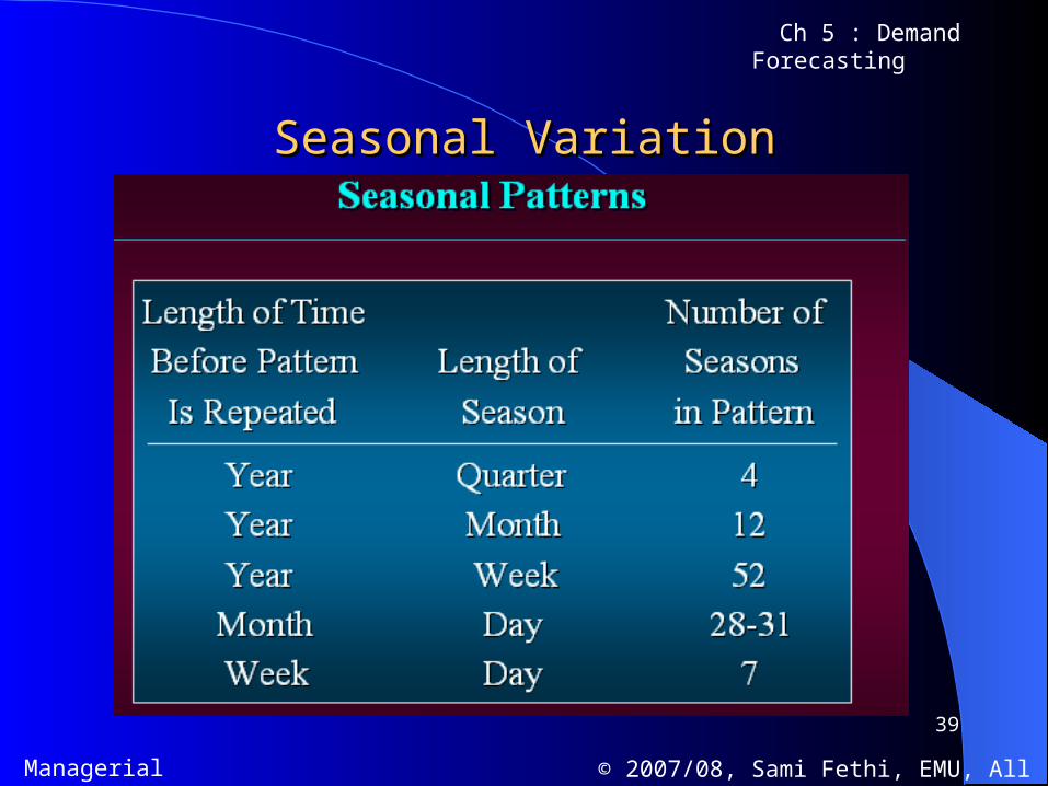
Reasons for Fluctuations in Time Series DataReasons for Fluctuations in Time Series Data
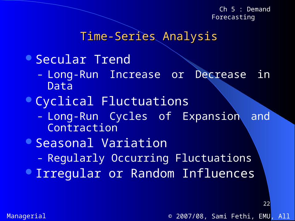
Secular Trend are noted by an upward or downward sloping line.
Cycle fluctuations is a data pattern that may cover several years before it repeats itself.
Seasonality is a data pattern that repeats itself over the period of one year or less.
Random influences (noise) results from random variation or unexplained causes.
22
Managerial Economics © 2007/08, Sami Fethi, EMU, All Right Reserved.
Ch 5 : Demand Forecasting
Time-Series AnalysisTime-Series Analysis
Secular Trend– Long-Run Increase or Decrease in Data
Cyclical Fluctuations– Long-Run Cycles of Expansion and
ContractionSeasonal Variation
– Regularly Occurring FluctuationsIrregular or Random Influences

23
Managerial Economics © 2007/08, Sami Fethi, EMU, All Right Reserved.
Ch 5 : Demand Forecasting
24
Managerial Economics © 2007/08, Sami Fethi, EMU, All Right Reserved.
Ch 5 : Demand Forecasting
25
Managerial Economics © 2007/08, Sami Fethi, EMU, All Right Reserved.
Ch 5 : Demand Forecasting
Trend ProjectionTrend Projection
The simplest form of time series is projecting the past trend by fitting a straight line to the data either visually or more precisely by regression analysis.

26
Managerial Economics © 2007/08, Sami Fethi, EMU, All Right Reserved.
Ch 5 : Demand Forecasting
Trend ProjectionTrend Projection- - Simple Linear RegressionSimple Linear Regression
Linear regression analysis establishes a relationship between a dependent variable and one or more independent variables.
In simple linear regression analysis there is only one independent variable.
If the data is a time series, the independent variable is the time period.
The dependent variable is whatever we wish to forecast.
27
Managerial Economics © 2007/08, Sami Fethi, EMU, All Right Reserved.
Ch 5 : Demand Forecasting
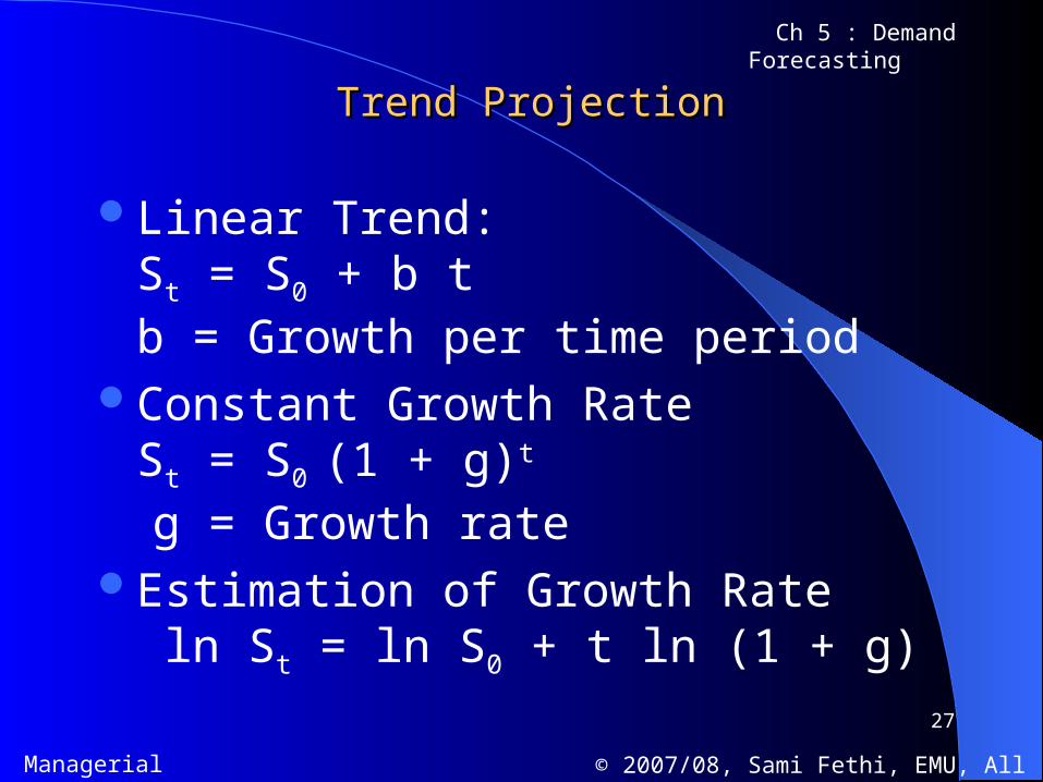
Trend ProjectionTrend Projection
Linear Trend:St = S0 + b tb = Growth per time period
Constant Growth RateSt = S0 (1 + g)t
g = Growth rateEstimation of Growth Rate
ln St = ln S0 + t ln (1 + g)
28
Managerial Economics © 2007/08, Sami Fethi, EMU, All Right Reserved.
Ch 5 : Demand Forecasting
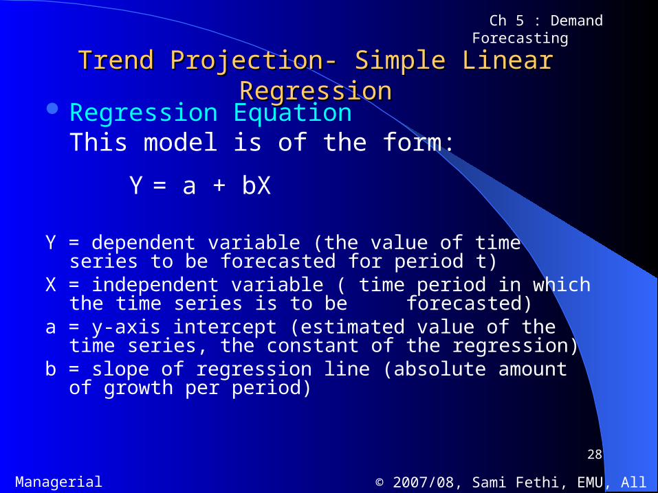
Trend ProjectionTrend Projection- - Simple Linear RegressionSimple Linear Regression Regression Equation
This model is of the form:
Y = a + bX
Y = dependent variable (the value of time series to be forecasted for period t)
X = independent variable ( time period in which the time series is to be forecasted)
a = y-axis intercept (estimated value of the time series, the constant of the regression)
b = slope of regression line (absolute amount of growth per period)
29
Managerial Economics © 2007/08, Sami Fethi, EMU, All Right Reserved.
Ch 5 : Demand Forecasting
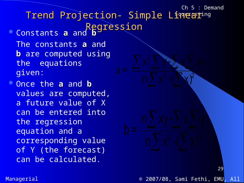
Trend ProjectionTrend Projection- - Simple Linear RegressionSimple Linear Regression Constants a a and bb
The constants aa and bb are computed using the equations given:
Once the a a and b b values are computed, a future value of X can be entered into the regression equation and a corresponding value of Y (the forecast) can be calculated.
2
2 2
x y- x xya =
n x -( x)
2 2
xy- x yb =
n x -( x)
n
30
Managerial Economics © 2007/08, Sami Fethi, EMU, All Right Reserved.
Ch 5 : Demand Forecasting
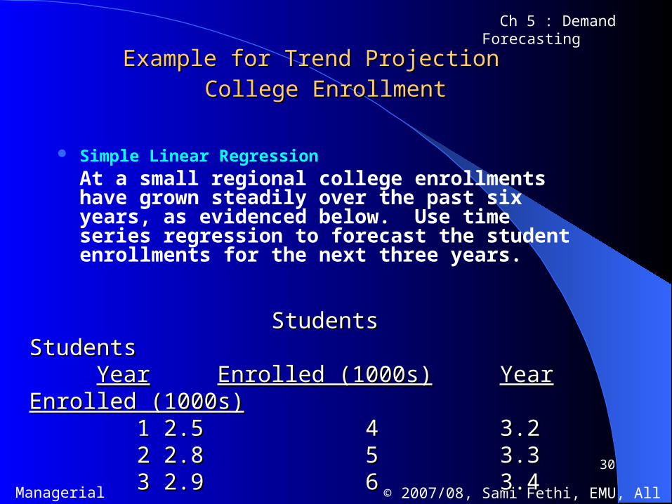
Example for Trend ProjectionExample for Trend Projection
College EnrollmentCollege Enrollment
Simple Linear Regression
At a small regional college enrollments have grown steadily over the past six years, as evidenced below. Use time series regression to forecast the student enrollments for the next three years.
StudentsStudents StudentsStudentsYearYear Enrolled (1000s)Enrolled (1000s) YearYear Enrolled (1000s)Enrolled (1000s) 11 2.52.5 44 3.23.2 22 2.82.8 55 3.33.3 33 2.92.9 66 3.43.4
31
Managerial Economics © 2007/08, Sami Fethi, EMU, All Right Reserved.
Ch 5 : Demand Forecasting
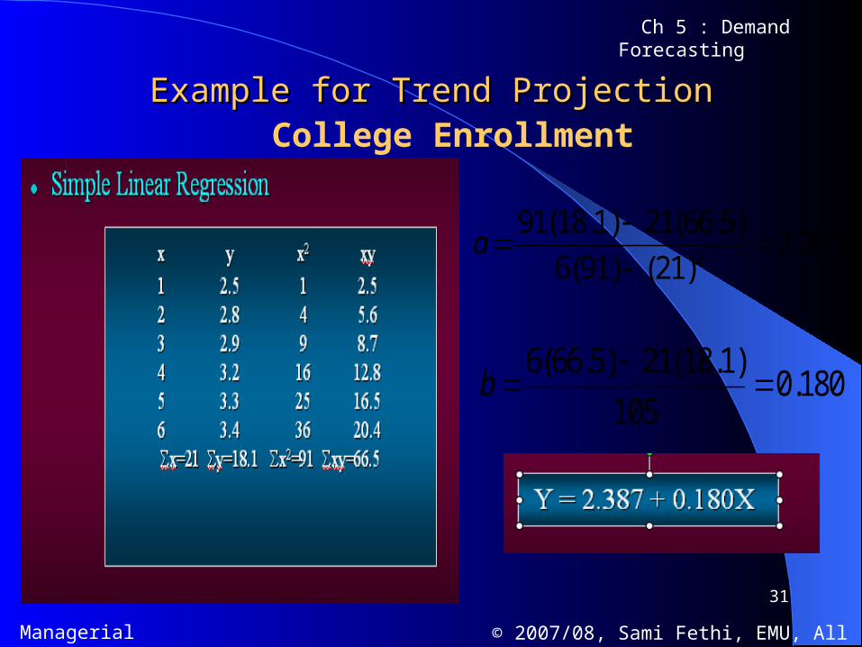
Example for Trend ProjectionExample for Trend Projection College Enrollment
2
91(18.1) 21(66.5)2.387
6(91) (21)a
6(66.5) 21(18.1)0.180
105b
32
Managerial Economics © 2007/08, Sami Fethi, EMU, All Right Reserved.
Ch 5 : Demand Forecasting
Example for Trend ProjectionExample for Trend Projection College EnrollmentCollege Enrollment
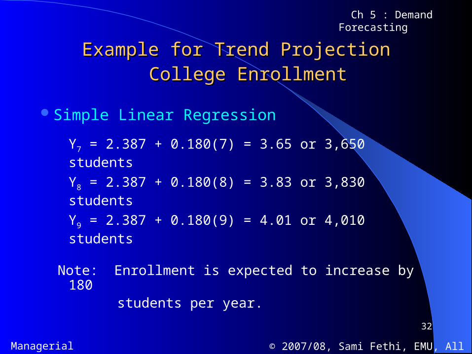
Simple Linear Regression
Y7 = 2.387 + 0.180(7) = 3.65 or 3,650 students
Y8 = 2.387 + 0.180(8) = 3.83 or 3,830 students
Y9 = 2.387 + 0.180(9) = 4.01 or 4,010 students
Note: Enrollment is expected to increase by 180 students per year.
33
Managerial Economics © 2007/08, Sami Fethi, EMU, All Right Reserved.
Ch 5 : Demand Forecasting
Example for Trend ProjectionExample for Trend Projection- - EElectricity saleslectricity sales
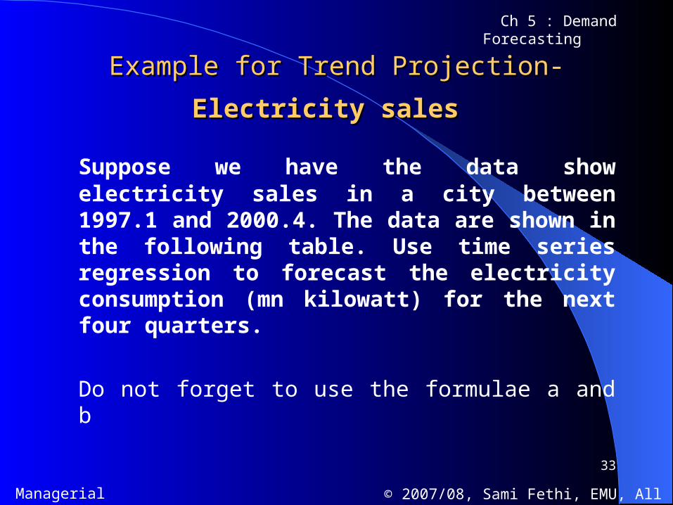
Suppose we have the data show electricity sales in a city between 1997.1 and 2000.4. The data are shown in the following table. Use time series regression to forecast the electricity consumption (mn kilowatt) for the next four quarters.
Do not forget to use the formulae a and b
34
Managerial Economics © 2007/08, Sami Fethi, EMU, All Right Reserved.
Ch 5 : Demand Forecasting
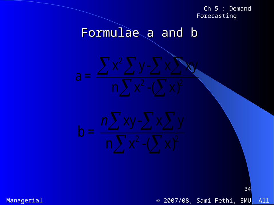
Formulae a and bFormulae a and b
2
2 2
x y- x xya =
n x -( x)
2 2
xy- x yb =
n x -( x)
n
35
Managerial Economics © 2007/08, Sami Fethi, EMU, All Right Reserved.
Ch 5 : Demand Forecasting
Example for Trend ProjectionExample for Trend Projection
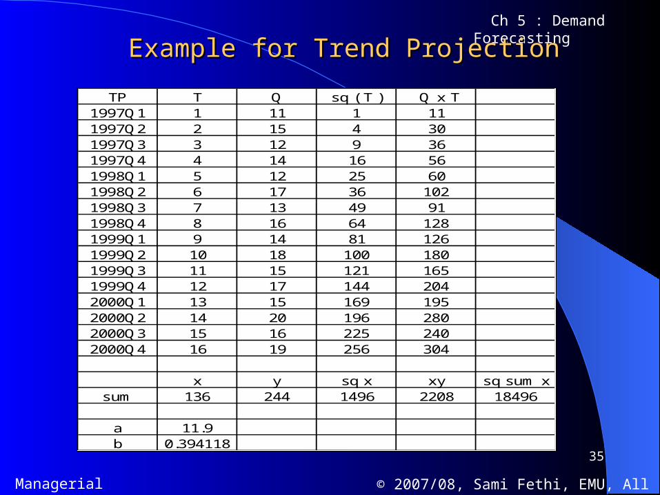
TP T Q sq ( T ) Q x T1997Q1 1 11 1 111997Q2 2 15 4 301997Q3 3 12 9 361997Q4 4 14 16 561998Q1 5 12 25 601998Q2 6 17 36 1021998Q3 7 13 49 911998Q4 8 16 64 1281999Q1 9 14 81 1261999Q2 10 18 100 1801999Q3 11 15 121 1651999Q4 12 17 144 2042000Q1 13 15 169 1952000Q2 14 20 196 2802000Q3 15 16 225 2402000Q4 16 19 256 304
x y sq x xy sq sum xsum 136 244 1496 2208 18496
a 11.9b 0.394118
36
Managerial Economics © 2007/08, Sami Fethi, EMU, All Right Reserved.
Ch 5 : Demand Forecasting
Example for Trend ProjectionExample for Trend Projection
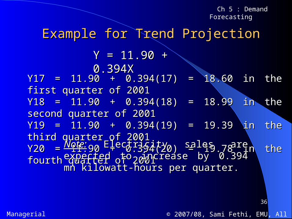
Y = 11.90 + 0.394XY = 11.90 + 0.394X
Y17 = 11.90 + 0.394(17) = 18.60 in the first quarter of 2001Y17 = 11.90 + 0.394(17) = 18.60 in the first quarter of 2001Y18 = 11.90 + 0.394(18) = 18.99 in the second quarter of 2001Y18 = 11.90 + 0.394(18) = 18.99 in the second quarter of 2001Y19 = 11.90 + 0.394(19) = 19.39 in the third quarter of 2001Y19 = 11.90 + 0.394(19) = 19.39 in the third quarter of 2001Y20 = 11.90 + 0.394(20) = 19.78 in the fourth quarter of 2001Y20 = 11.90 + 0.394(20) = 19.78 in the fourth quarter of 2001
Note:Note: Electricity sales are expected to increase Electricity sales are expected to increase by 0.394 mn kilowatt-hours per quarter.by 0.394 mn kilowatt-hours per quarter.
37
Managerial Economics © 2007/08, Sami Fethi, EMU, All Right Reserved.
Ch 5 : Demand Forecasting
Example for Trend Projection using Example for Trend Projection using S Stt = S = S0 0 (1 + g)(1 + g)tt
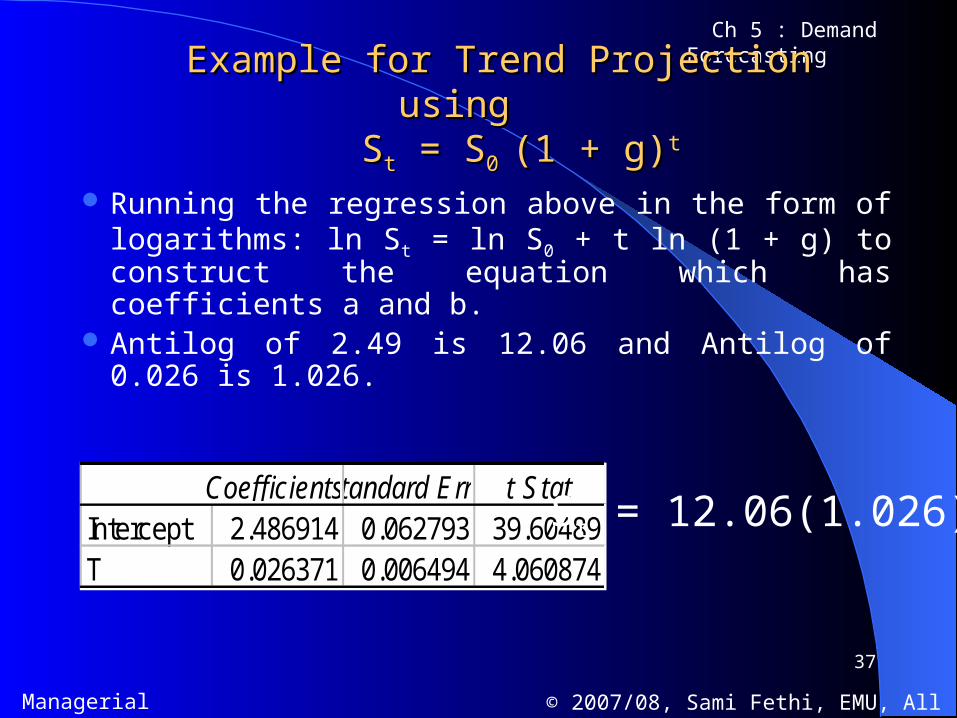
Running the regression above in the form of logarithms: ln St = ln S0 + t ln (1 + g) to construct the equation which has coefficients a and b.
Antilog of 2.49 is 12.06 and Antilog of 0.026 is 1.026.
CoefficientsStandard Error t StatIntercept 2.486914 0.062793 39.60489T 0.026371 0.006494 4.060874
St = 12.06(1.026)t
38
Managerial Economics © 2007/08, Sami Fethi, EMU, All Right Reserved.
Ch 5 : Demand Forecasting
Example for Trend Projection using Example for Trend Projection using S Stt = S = S0 0 (1 + g)(1 + g)tt
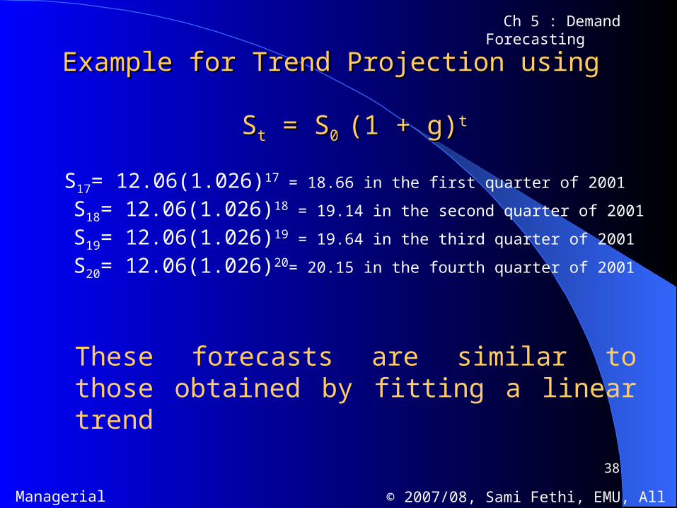
S17= 12.06(1.026)17 = 18.66 in the first quarter of 2001
S18= 12.06(1.026)18 = 19.14 in the second quarter of 2001
S19= 12.06(1.026)19 = 19.64 in the third quarter of 2001
S20= 12.06(1.026)20= 20.15 in the fourth quarter of 2001
These forecasts are similar to those obtained by fitting a linear trend
39
Managerial Economics © 2007/08, Sami Fethi, EMU, All Right Reserved.
Ch 5 : Demand Forecasting
Seasonal VariationSeasonal Variation
40
Managerial Economics © 2007/08, Sami Fethi, EMU, All Right Reserved.
Ch 5 : Demand Forecasting
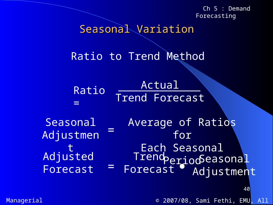
Seasonal VariationSeasonal Variation
Ratio to Trend Method
ActualTrend Forecast
Ratio =
SeasonalAdjustment =
Average of Ratios forEach Seasonal Period
AdjustedForecast =
TrendForecast
SeasonalAdjustment

41
Managerial Economics © 2007/08, Sami Fethi, EMU, All Right Reserved.
Ch 5 : Demand Forecasting
SeasonalSeasonal Variation Variation
Ratio to Trend Method:Example Calculation for Quarter 1
Trend Forecast for 2001.1 = 11.90 + (0.394)(17) = 18.60
Seasonally Adjusted Forecast for 2001.1 = (18.60)(0.887) = 16.50
YEAR Forecasted Actual Act/Forec1997Q1 12.29 11 0.8950371998Q1 13.87 12 0.8651771999Q1 15.45 14 0.9061492000Q1 17.02 15 0.881316
AV 0.886920.887

42
Managerial Economics © 2007/08, Sami Fethi, EMU, All Right Reserved.
Ch 5 : Demand Forecasting
Seasonal VariationSeasonal Variation
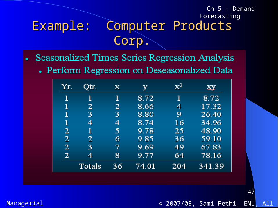
Select a representative historical data set. Develop a seasonal index for each season. Use the seasonal indexes to deseasonalize the data. Perform linear regression analysis on the
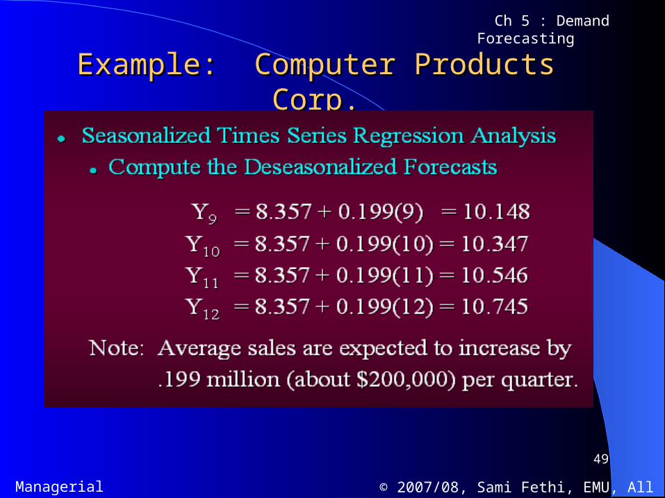
deseasonalized data. Use the regression equation to compute the
forecasts. Use the seas. indexes to reapply the seasonal
patterns to the forecasts.
43
Managerial Economics © 2007/08, Sami Fethi, EMU, All Right Reserved.
Ch 5 : Demand Forecasting
Example: Computer Products Corp.Example: Computer Products Corp.Seasonalized Times Series Regression
Analysis
An analyst at CPC wants to develop next year’s quarterly forecasts of sales revenue for CPC’s line of Epsilon Computers. The analyst believes that the most recent 8 quarters of sales (shown on the next slide) are representative of next year’s sales.

44
Managerial Economics © 2007/08, Sami Fethi, EMU, All Right Reserved.
Ch 5 : Demand Forecasting
Example: Computer Products Corp.Example: Computer Products Corp.

45
Managerial Economics © 2007/08, Sami Fethi, EMU, All Right Reserved.
Ch 5 : Demand Forecasting
Example: Computer Products Corp.Example: Computer Products Corp.

46
Managerial Economics © 2007/08, Sami Fethi, EMU, All Right Reserved.
Ch 5 : Demand Forecasting
Example: Computer Products Corp.Example: Computer Products Corp.
47
Managerial Economics © 2007/08, Sami Fethi, EMU, All Right Reserved.
Ch 5 : Demand Forecasting
Example: Computer Products Corp.Example: Computer Products Corp.

48
Managerial Economics © 2007/08, Sami Fethi, EMU, All Right Reserved.
Ch 5 : Demand Forecasting
Example: Computer Products Corp.Example: Computer Products Corp.
49
Managerial Economics © 2007/08, Sami Fethi, EMU, All Right Reserved.
Ch 5 : Demand Forecasting
Example: Computer Products Corp.Example: Computer Products Corp.

50
Managerial Economics © 2007/08, Sami Fethi, EMU, All Right Reserved.
Ch 5 : Demand Forecasting
Smoothing TechniquesSmoothing Techniques
Smoothing techniques are useful when the time series exhibit little trend or seasonal variations.
(Simple) Moving Average Weighted Moving Average Exponential Smoothing Exponential Smoothing with Trend

51
Managerial Economics © 2007/08, Sami Fethi, EMU, All Right Reserved.
Ch 5 : Demand Forecasting
Simple Moving AverageSimple Moving Average
An averaging period (AP) is given or selected The forecast for the next period is the arithmetic average of
the AP most recent actual demands It is called a “simple” average because each period used to
compute the average is equally weighted It is called “moving” because as new demand data becomes
available, the oldest data is not used By increasing the AP, the forecast is less responsive to
fluctuations in demand (low impulse response and high noise dampening)
By decreasing the AP, the forecast is more responsive to fluctuations in demand (high impulse response and low noise dampening)

52
Managerial Economics © 2007/08, Sami Fethi, EMU, All Right Reserved.
Ch 5 : Demand Forecasting
Moving Average ForecastsMoving Average Forecasts-Formula-Formula
Forecast is the average of data from w periods prior to the forecast data point.
1
wt i
ti
AF
w
It is It is called “moving” because as new demand data becomes available, the oldest data is not used used
53
Managerial Economics © 2007/08, Sami Fethi, EMU, All Right Reserved.
Ch 5 : Demand Forecasting
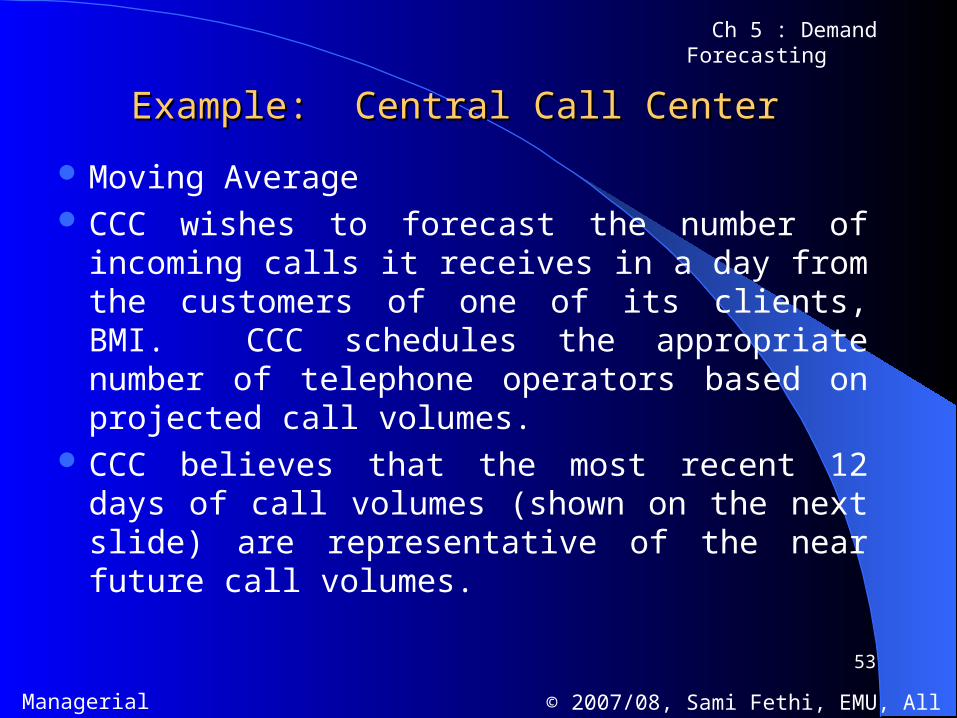
Example: Central Call CenterExample: Central Call Center
Moving Average CCC wishes to forecast the number of incoming
calls it receives in a day from the customers of one of its clients, BMI. CCC schedules the appropriate number of telephone operators based on projected call volumes.
CCC believes that the most recent 12 days of call volumes (shown on the next slide) are representative of the near future call volumes.

54
Managerial Economics © 2007/08, Sami Fethi, EMU, All Right Reserved.
Ch 5 : Demand Forecasting
Example: Central Call CenterExample: Central Call Center
55
Managerial Economics © 2007/08, Sami Fethi, EMU, All Right Reserved.
Ch 5 : Demand Forecasting
Example: Central Call CenterExample: Central Call Center
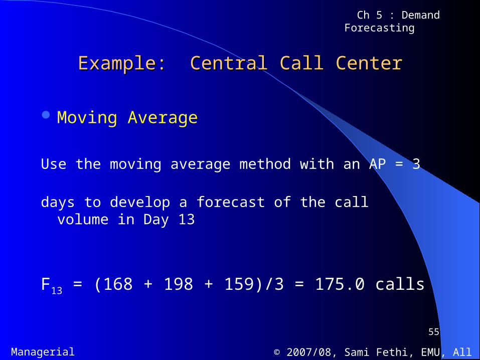
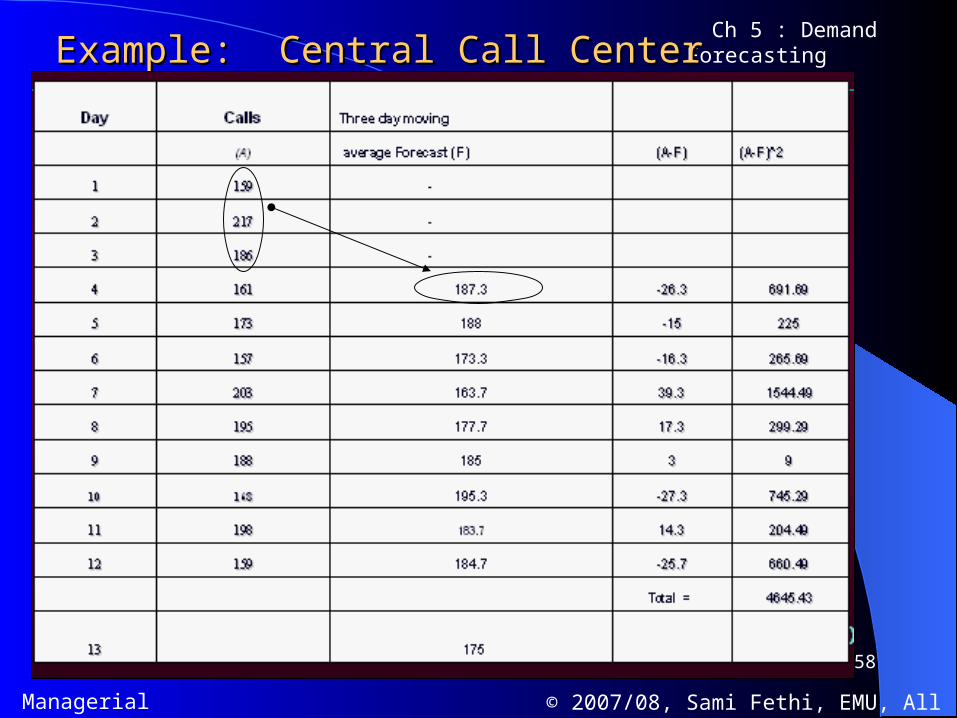
Moving Average
Use the moving average method with an AP = 3
days to develop a forecast of the call volume in Day 13
F13 = (168 + 198 + 159)/3 = 175.0 calls

56
Managerial Economics © 2007/08, Sami Fethi, EMU, All Right Reserved.
Ch 5 : Demand Forecasting
Evaluating Forecast-Model PerformanceEvaluating Forecast-Model Performance
Accuracy– Accuracy is the typical criterion for judging the performance of a
forecasting approach– Accuracy is how well the forecasted values match the actual values
Accuracy of a forecasting approach needs to be monitored to assess the confidence you can have in its forecasts and changes in the market may require reevaluation of the approach
Accuracy can be measured in several ways– Standard error of the forecast – Mean absolute deviation (MAD)– Mean squared error (MSE)
57
Managerial Economics © 2007/08, Sami Fethi, EMU, All Right Reserved.
Ch 5 : Demand Forecasting
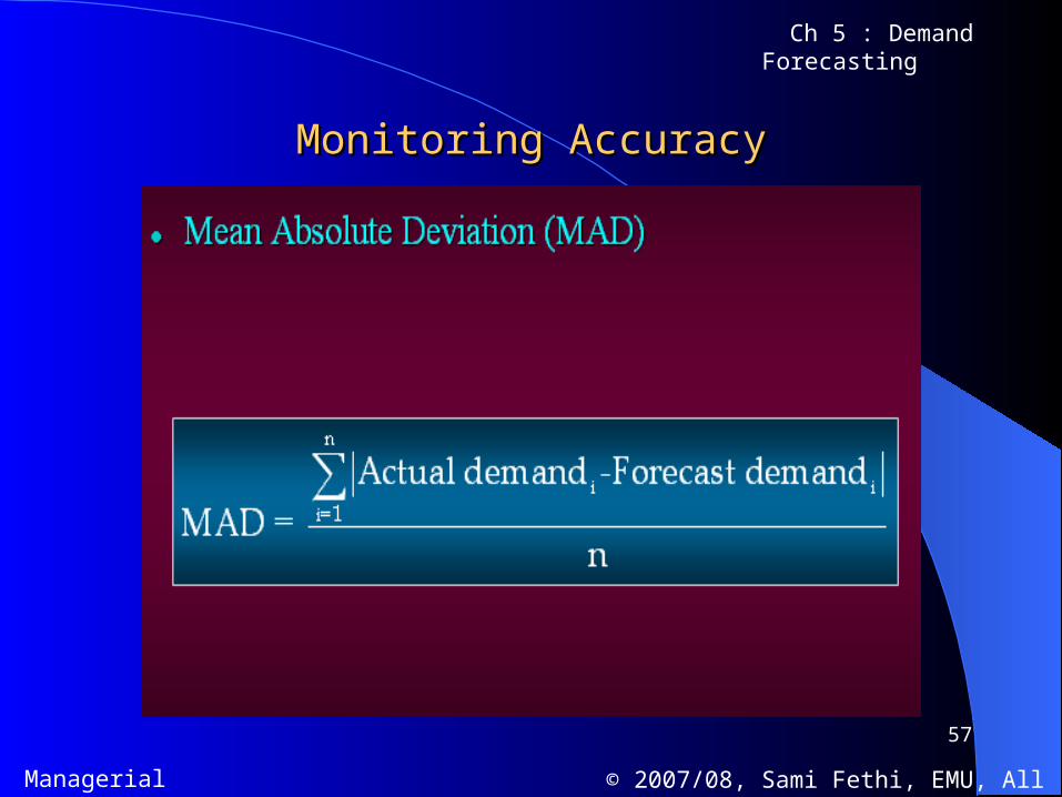
Monitoring AccuracyMonitoring Accuracy
58
Managerial Economics © 2007/08, Sami Fethi, EMU, All Right Reserved.
Ch 5 : Demand Forecasting Example: Central Call CenterExample: Central Call Center
59
Managerial Economics © 2007/08, Sami Fethi, EMU, All Right Reserved.
Ch 5 : Demand Forecasting
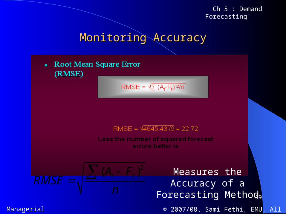
Monitoring AccuracyMonitoring Accuracy
2( )t tA FRMSE
n
Measures the Accuracy
of a Forecasting Method
60
Managerial Economics © 2007/08, Sami Fethi, EMU, All Right Reserved.
Ch 5 : Demand Forecasting
Weighted Moving AverageWeighted Moving Average
This is a variation on the simple moving average where the weights used to compute the average are not equal.
This allows more recent demand data to have a greater effect on the moving average, therefore the forecast.
The weights must add to 1.0 and generally decrease in value with the age of the data.
The distribution of the weights determine the impulse response of the forecast.
61
Managerial Economics © 2007/08, Sami Fethi, EMU, All Right Reserved.
Ch 5 : Demand Forecasting
Example: Central Call CenterExample: Central Call Center
Weighted Moving Average Use the weighted moving average method with an AP = 3
days and weights of .1 (for oldest datum), .3, and .6 to develop a forecast of the call volume in Day 13.
F13 = .1(168) + .3(198) + .6(159) = 171.6 calls
Note: The WMA forecast is lower than the MA forecast because Day 13’s relatively low call volume carries almost twice as much weight in the WMA (.60) as it does in the MA (.33).

62
Managerial Economics © 2007/08, Sami Fethi, EMU, All Right Reserved.
Ch 5 : Demand Forecasting
Exponential SmoothingExponential SmoothingForecastsForecasts
1 (1 )t t tF wA w F
Forecast is the weighted average of the forecast and the actual value from the prior period.
0 1w
63
Managerial Economics © 2007/08, Sami Fethi, EMU, All Right Reserved.
Ch 5 : Demand Forecasting
Exponential SmoothingExponential SmoothingForecastsForecasts
The weights used to compute the forecast (moving average) are exponentially distributed.
The forecast is the sum of the old forecast and a portion () of the forecast error (A t-1-Ft-1).
The smoothing constant, , must be between 0.0 and 1.0.
A large provides a high impulse response forecast. A small provides a low impulse response forecast.
64
Managerial Economics © 2007/08, Sami Fethi, EMU, All Right Reserved.
Ch 5 : Demand Forecasting Example: Central Call CenterExample: Central Call Center
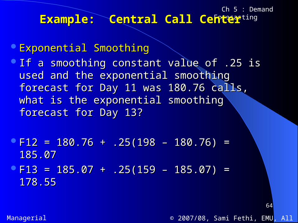
Exponential SmoothingExponential SmoothingIf a smoothing constant value of .25 is used If a smoothing constant value of .25 is used
and the exponential smoothing forecast for and the exponential smoothing forecast for Day 11 was 180.76 calls, what is the Day 11 was 180.76 calls, what is the exponential smoothing forecast for Day 13?exponential smoothing forecast for Day 13?
F12 = 180.76 + .25(198 – 180.76) = 185.07F12 = 180.76 + .25(198 – 180.76) = 185.07F13 = 185.07 + .25(159 – 185.07) = 178.55F13 = 185.07 + .25(159 – 185.07) = 178.55
65
Managerial Economics © 2007/08, Sami Fethi, EMU, All Right Reserved.
Ch 5 : Demand Forecasting
Example: Central Call CenterExample: Central Call Center
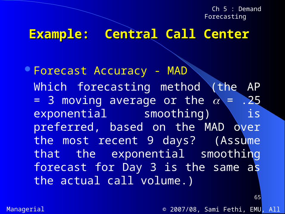
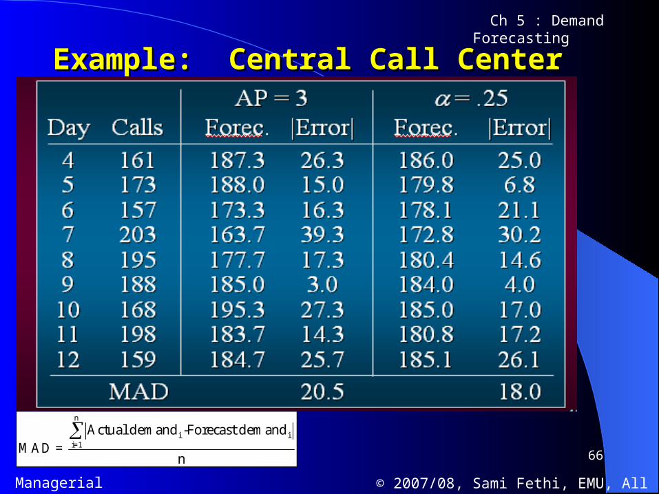
Forecast Accuracy - MAD
Which forecasting method (the AP = 3 moving average or the = .25 exponential smoothing) is preferred, based on the MAD over the most recent 9 days? (Assume that the exponential smoothing forecast for Day 3 is the same as the actual call volume.)
66
Managerial Economics © 2007/08, Sami Fethi, EMU, All Right Reserved.
Ch 5 : Demand Forecasting
Example: Central Call CenterExample: Central Call Center
n
i ii=1
Actual demand -Forecast demandMAD =
n
67
Managerial Economics © 2007/08, Sami Fethi, EMU, All Right Reserved.
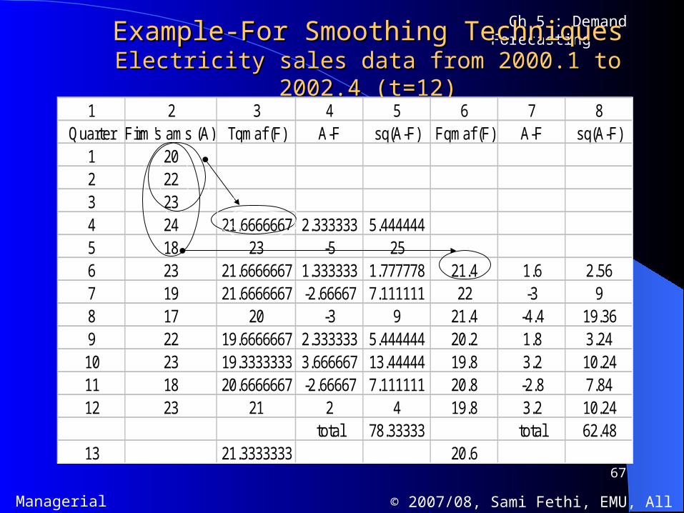
Ch 5 : Demand Forecasting ExampleExample--For Smoothing TechniquesFor Smoothing Techniques
Electricity sales data from 2000.1 to 2002.4 (t=12)Electricity sales data from 2000.1 to 2002.4 (t=12)
1 2 3 4 5 6 7 8Quarter Firm's ams (A) Tqmaf (F) A-F sq(A-F) Fqmaf (F) A-F sq(A-F)
1 202 223 234 24 21.6666667 2.333333 5.4444445 18 23 -5 256 23 21.6666667 1.333333 1.777778 21.4 1.6 2.567 19 21.6666667 -2.66667 7.111111 22 -3 98 17 20 -3 9 21.4 -4.4 19.369 22 19.6666667 2.333333 5.444444 20.2 1.8 3.2410 23 19.3333333 3.666667 13.44444 19.8 3.2 10.2411 18 20.6666667 -2.66667 7.111111 20.8 -2.8 7.8412 23 21 2 4 19.8 3.2 10.24
total 78.33333 total 62.4813 21.3333333 20.6
68
Managerial Economics © 2007/08, Sami Fethi, EMU, All Right Reserved.
Ch 5 : Demand Forecasting
Example For Smoothing TechniquesExample For Smoothing Techniques
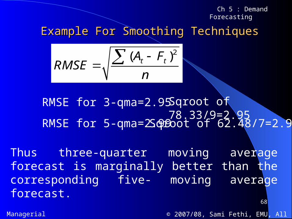
2( )t tA FRMSE
n
RMSE for 3-qma=2.95
RMSE for 5-qma=2.99
Thus three-quarter moving average forecast is marginally better than the corresponding five- moving average forecast.
Sqroot of 78.33/9=2.95
Sqroot of 62.48/7=2.98
69
Managerial Economics © 2007/08, Sami Fethi, EMU, All Right Reserved.
Ch 5 : Demand Forecasting
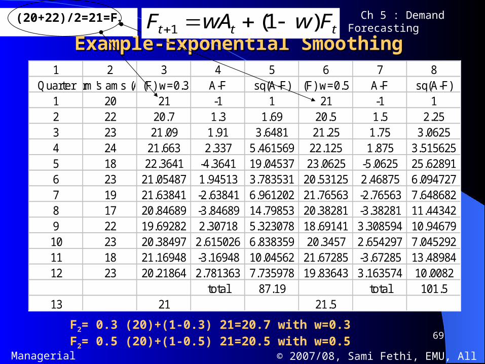
Example-Exponential SmoothingExample-Exponential Smoothing1 2 3 4 5 6 7 8
QuarterFirm's ams (A) (F) w=0.3 A-F sq(A-F) (F) w=0.5 A-F sq(A-F)1 20 21 -1 1 21 -1 12 22 20.7 1.3 1.69 20.5 1.5 2.253 23 21.09 1.91 3.6481 21.25 1.75 3.06254 24 21.663 2.337 5.461569 22.125 1.875 3.5156255 18 22.3641 -4.3641 19.04537 23.0625 -5.0625 25.628916 23 21.05487 1.94513 3.783531 20.53125 2.46875 6.0947277 19 21.63841 -2.63841 6.961202 21.76563 -2.76563 7.6486828 17 20.84689 -3.84689 14.79853 20.38281 -3.38281 11.443429 22 19.69282 2.30718 5.323078 18.69141 3.308594 10.9467910 23 20.38497 2.615026 6.838359 20.3457 2.654297 7.04529211 18 21.16948 -3.16948 10.04562 21.67285 -3.67285 13.4898412 23 20.21864 2.781363 7.735978 19.83643 3.163574 10.0082
total 87.19 total 101.513 21 21.5
F2= 0.3 (20)+(1-0.3) 21=20.7 with w=0.3F2= 0.5 (20)+(1-0.5) 21=20.5 with w=0.5
(20+22)/2=21=F11 (1 )t t tF wA w F

70
Managerial Economics © 2007/08, Sami Fethi, EMU, All Right Reserved.
Ch 5 : Demand Forecasting
Example-Exponential SmoothingExample-Exponential Smoothing
F2= 0.3 (20)+(1-0.3) 21=20.7 with w=0.3
F2= 0.5 (20)+(1-0.5) 21=20.5 with w=0.5
RMSE with w=0.3 is 2.70 RMSE with w=0.5 is 2.91
Both exponential forecasts are better than the previous techniques in terms of average values.
71
Managerial Economics © 2007/08, Sami Fethi, EMU, All Right Reserved.
Ch 5 : Demand Forecasting
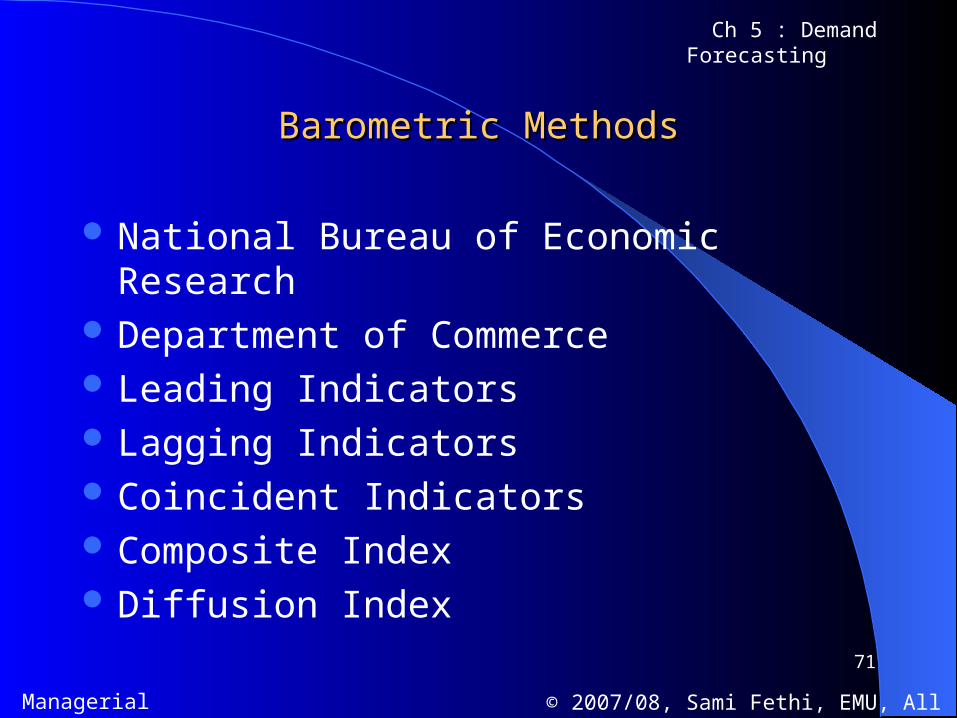
Barometric MethodsBarometric Methods
National Bureau of Economic Research Department of Commerce Leading Indicators Lagging Indicators Coincident Indicators Composite Index Diffusion Index
72
Managerial Economics © 2007/08, Sami Fethi, EMU, All Right Reserved.
Ch 5 : Demand Forecasting
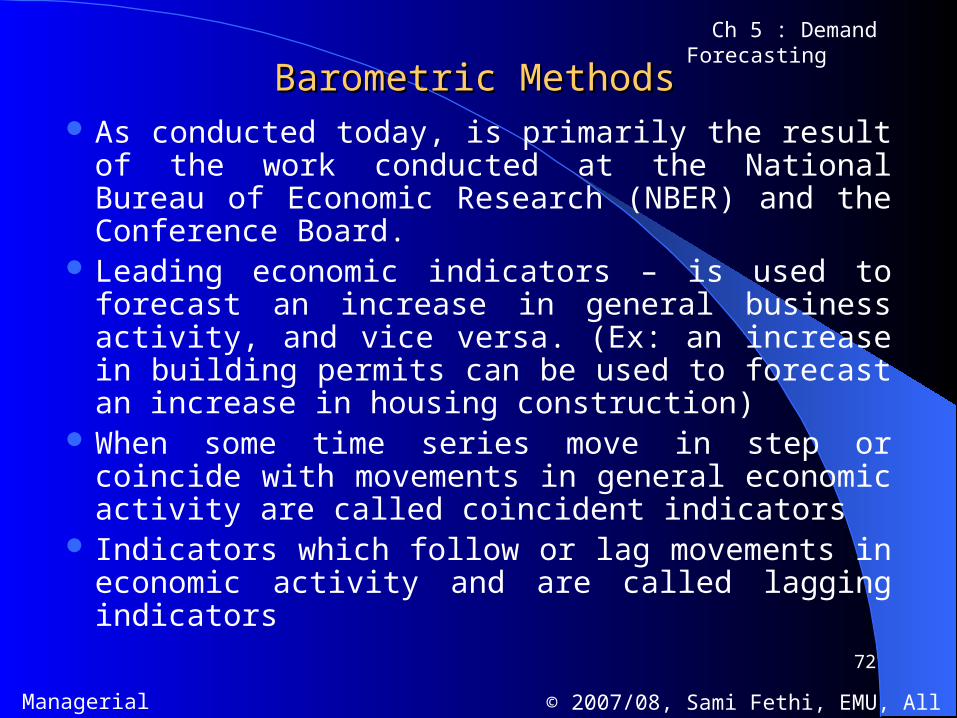
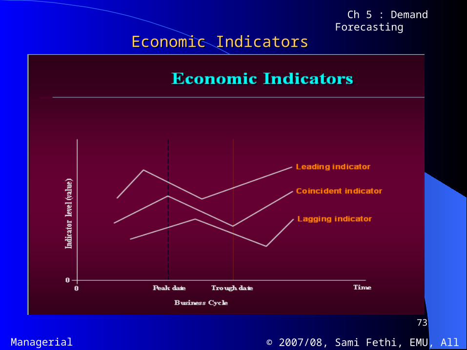
Barometric MethodsBarometric Methods As conducted today, is primarily the result of the
work conducted at the National Bureau of Economic Research (NBER) and the Conference Board.
Leading economic indicators – is used to forecast an increase in general business activity, and vice versa. (Ex: an increase in building permits can be used to forecast an increase in housing construction)
When some time series move in step or coincide with movements in general economic activity are called coincident indicators
Indicators which follow or lag movements in economic activity and are called lagging indicators
73
Managerial Economics © 2007/08, Sami Fethi, EMU, All Right Reserved.
Ch 5 : Demand Forecasting
Economic IndicatorsEconomic Indicators

74
Managerial Economics © 2007/08, Sami Fethi, EMU, All Right Reserved.
Ch 5 : Demand Forecasting
Leading indicators (10 series)
Average weekly hours, manufacturing
Initial claims for unemployment insurance, thousands
Manufacturers’ new orders, consumer goods and materials
Vendor performance, slower deliveries diffusion index
Manufacturers’ new orders, nondefense capital goods
Building permits, new private housing units
Stock prices, 500 common stocks
Money supply, M2
Interest rate spread, 10-year Treasury bonds less federal funds
Index of consumer expectations
75
Managerial Economics © 2007/08, Sami Fethi, EMU, All Right Reserved.
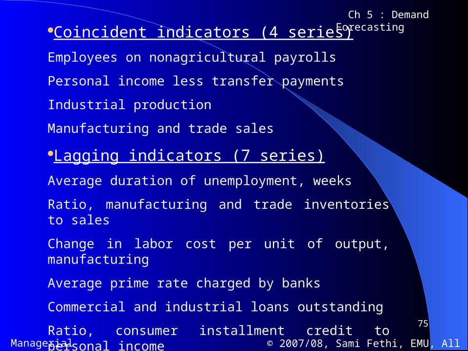
Ch 5 : Demand Forecasting Coincident indicators (4 series)
Employees on nonagricultural payrolls
Personal income less transfer payments
Industrial production
Manufacturing and trade sales
Lagging indicators (7 series)
Average duration of unemployment, weeks
Ratio, manufacturing and trade inventories to sales
Change in labor cost per unit of output, manufacturing
Average prime rate charged by banks
Commercial and industrial loans outstanding
Ratio, consumer installment credit to personal income
Change in consumer price index for services

76
Managerial Economics © 2007/08, Sami Fethi, EMU, All Right Reserved.
Ch 5 : Demand Forecasting
Econometric ModelsEconometric Models The characteristic that distinguishes econometric
model from other forecasting methods is that they seek to identify and measure the relative importance (elasticity) of the various determinants of demand or other economic variables to be forecasted.
Econometric forecasting frequently incorporates or uses the best features of other forecasting techniques, such as trend and seasonal variations, smoothing techniques, and leading indicators
77
Managerial Economics © 2007/08, Sami Fethi, EMU, All Right Reserved.
Ch 5 : Demand Forecasting
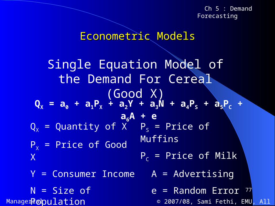
Econometric ModelsEconometric Models
Single Equation Model of the Demand For Cereal (Good X)
QX = a0 + a1PX + a2Y + a3N + a4PS + a5PC + a6A + e
QX = Quantity of X
PX = Price of Good X
Y = Consumer Income
N = Size of Population
PS = Price of Muffins
PC = Price of Milk
A = Advertising
e = Random Error
78
Managerial Economics © 2007/08, Sami Fethi, EMU, All Right Reserved.
Ch 5 : Demand Forecasting
Econometric ModelsEconometric Models
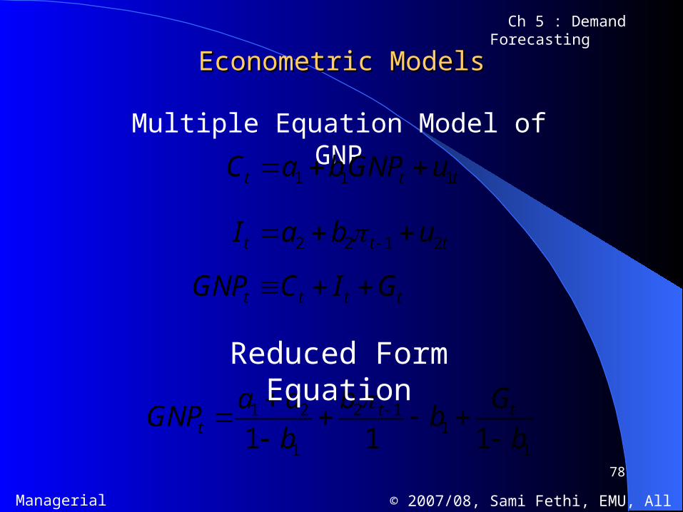
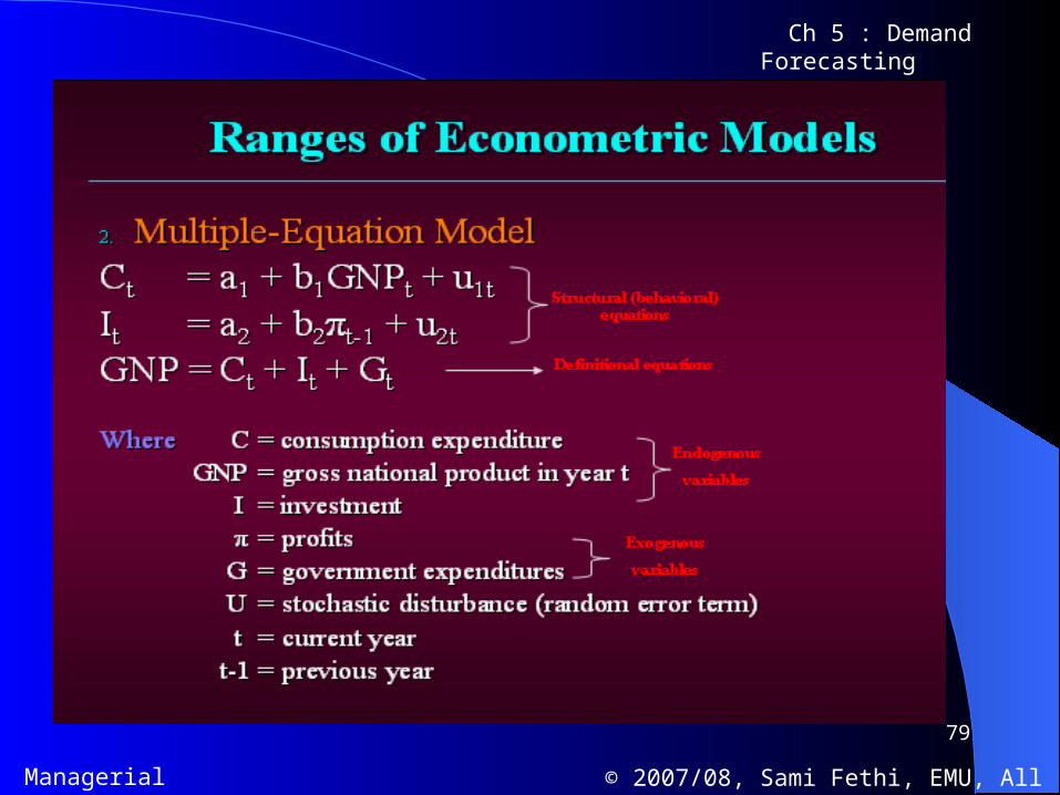
Multiple Equation Model of GNP
1 1 1t t tC a b GNP u
2 2 1 2t t tI a b u
t t t tGNP C I G
2 11 21
1 11 1 1t t
t
b Ga aGNP b
b b
Reduced Form Equation
79
Managerial Economics © 2007/08, Sami Fethi, EMU, All Right Reserved.
Ch 5 : Demand Forecasting

80
Managerial Economics © 2007/08, Sami Fethi, EMU, All Right Reserved.
Ch 5 : Demand Forecasting
Reasons for Ineffective ForecastingReasons for Ineffective Forecasting
Not involving a broad cross section of people Not recognizing that forecasting is integral to
business planning Not recognizing that forecasts will always be
wrong Not forecasting the right things Not selecting an appropriate forecasting method Not tracking the accuracy of the forecasting
models
81
Managerial Economics © 2007/08, Sami Fethi, EMU, All Right Reserved.
Ch 5 : Demand Forecasting
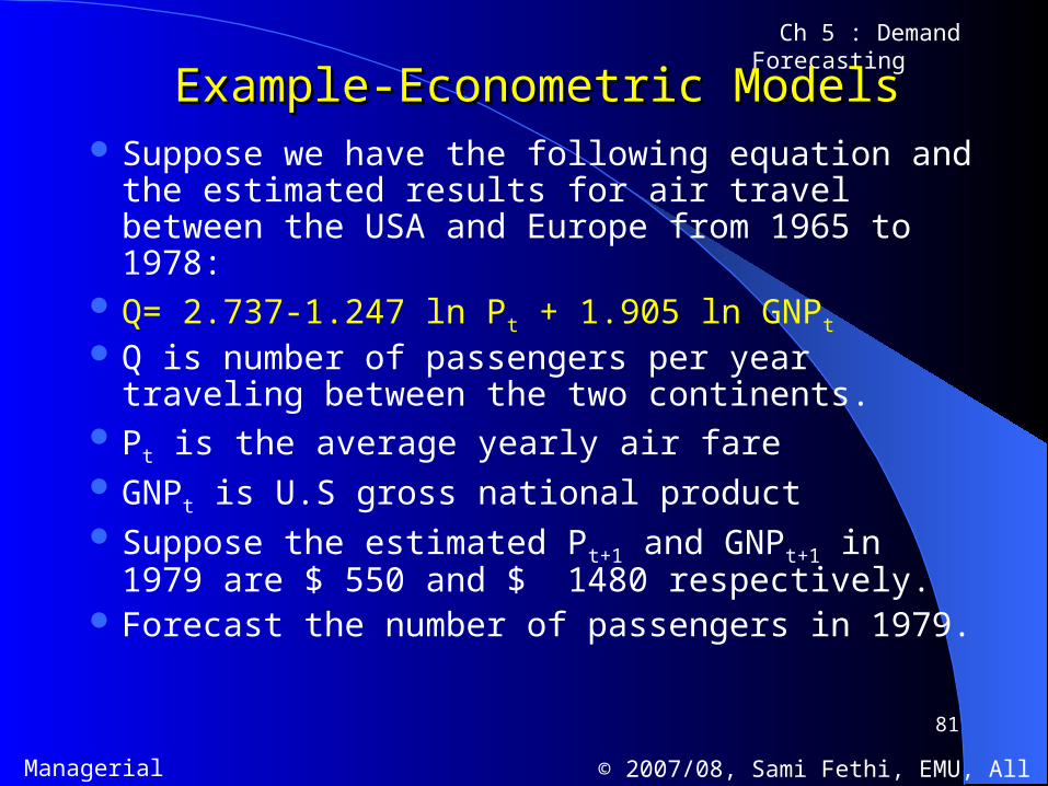
Example-Econometric ModelsExample-Econometric Models Suppose we have the following equation and the
estimated results for air travel between the USA and Europe from 1965 to 1978:
Q= 2.737-1.247 ln Pt + 1.905 ln GNPt
Q is number of passengers per year traveling between the two continents.
Pt is the average yearly air fare GNPt is U.S gross national product Suppose the estimated Pt+1 and GNPt+1 in 1979 are $
550 and $ 1480 respectively. Forecast the number of passengers in 1979.
82
Managerial Economics © 2007/08, Sami Fethi, EMU, All Right Reserved.
Ch 5 : Demand Forecasting
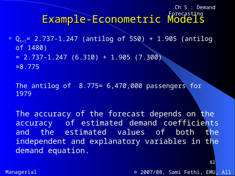
Example-Econometric ModelsExample-Econometric Models
Qt+1= 2.737-1.247 (antilog of 550) + 1.905 (antilog of 1480)
= 2.737-1.247 (6.310) + 1.905 (7.300)
=8.775
The antilog of 8.775= 6,470,000 passengers for 1979
The accuracy of the forecast depends on the accuracy of estimated demand coefficients and the estimated values of both the independent and explanatory variables in the demand equation.
83
Managerial Economics © 2007/08, Sami Fethi, EMU, All Right Reserved.
Ch 5 : Demand Forecasting
The EndThe End
Thanks