Department of Biostatistics University of Copenhagen

A note on the validity of the case-time-control design for autocorrelated exposure histories

Aksel K.G. Jensen

Thomas A. Gerds

Peter Weeke

Christian Torp-Pedersen

Per K. Andersen

Research Report 12/11

Department of Biostatistics University of Copenhagen

A note on the validity of the case-time-control design forautocorrelated exposure histories

Aksel K.G. Jensen1, Thomas A. Gerds1, Peter Weeke2, Christian Torp-Pedersen2, and PerK. Andersen1

1Department of Biostatistics, University of Copenhagen

2Department of Cardiology, Copenhagen University Hospital, Gentofte, Denmark

December 17, 2012

Abstract

The case-time-control design is an extension of the case-crossover design which handles timetrends in the exposure of the general population. As in the case-crossover design, time-invariantconfounders are controlled for by the design itself. The basic idea is to compare the exposurestatus of an individual in one or several reference periods where no event occurred to the expo-sure status of the same individual in the index period where the event occurred. By comparingcase-crossover results in cases to case-crossover results in controls exposure-outcome effectcan be estimated by conditional logistic regression. We review the mathematical assumptionsunderlying the case-time-control design. In addition we examine the sensitivity of the designto deviations from the assumed independence of within-individual exposure history. Resultsfrom simulating different scenarios suggest that the design is quite robust to deviations fromthis model assumption. A side result of our investigation shows that the development in ex-posure probability over time can be modelled in a flexible way, e.g. using polynomials orregression splines.

1

1 Introduction

Observational cohort studies play an important role for monitoring safety of drugs that have alreadybeen approved for marketing. In Weeke et al.1 we recently studied the association of prescriptionantidepressants and the risk of out-of-hospital cardiac arrest by means of the case-time-controldesign2. The case-time-control design is an extension of the popular case-crossover design. Re-sulting from an observational study, the results were under the suspicion of an increased risk of bias(compared to a randomized clinical trial). This prompted us to review the mathematical assump-tions underlying the case-time-control design.

The case-crossover design was introduced by Maclure3 to control for time constant subject charac-teristics in observational studies. The principle of the case-crossover design is to use cases as theirown controls by assessing exposure not only immediately prior to the case period but also prior toa suitably chosen earlier reference period where the event did not occur. The case-crossover designis useful if exposure varies over time and if the latency period from exposure to event is relativelyshort4. However, case-crossover results are known to be biased when there are time trends in thegeneral population exposure prevalence,5 and more generally when there are within-individual ex-posure dependencies6,7. Vines & Farrington6 pointed out that it is safe to analyse case-crossoverstudies with exactly one control period when there is pairwise exchangeability, which amounts toassuming that the marginal exposure probability is the same in the case period and in the controlperiod. However, when there are multiple control periods valid results can only be expected undera stronger global exchangeability condition, which practically amounts to assuming that all indi-vidual exposures across time are independent.

Weeke et al.1 studied also antidepressants that were newly introduced on the market. Thereafter,some of them showed strong general population time trends. This made a case-crossover analysisinappropriate, as the exposure effect would be confounded by the period effect. The case-time-control design2 was thus suggested to eliminate general population exposure time trends. It worksby including controls from the general population. A number M ≥ 1 of controls are matched toeach case and their exposure status is analysed in a numberK ≥ 1 of periods that are matched to theperiods of the corresponding case. As in the case-crossover design, time-invariant confounders arecontrolled for by the design itself. In addition, general population time trends can be distinguishedfrom exposure-outcome effects.

The purpose of the present work is threefold. First, we will clarify the assumptions leading toSuissa’s logistic model2 which combines a model for exposure time trends in the general popu-lation with a model for the association of exposure and the risk of an event. Second, we extendSuissa’s framework in several ways. We discuss the details of the design with two reference pe-riods. Furthermore, our exposure model includes time constant subject effects which are allowedto be different from the time constant subject effects on the event risk. Based on this model weare able to show that certain between-subject differences in exposure time trends will not introducebias. Another extension of practical and theoretical interest is that the exposure probability doesnot have to be linear. In fact it can be modelled as a function of time in a flexible way, e.g., byusing splines. This means that the placement of reference periods is not constrained to be equidis-

2

tant, and hence can be adapted to other features of the study, such as the nature of the exposure.Third, we show results from a simulation study on the sensitivity of the case-time-control designin situations where there besides a general population exposure time trend also are within-subjectexposure dependencies in the simulated data. To what extent the latter affect the results of the case-time-control analysis is not obvious. In particular not for multiple reference periods (K > 1) whichwas not explicitly discussed by Suissa.

For further discussion of the case-time-control design see also Suissa8 and Greenland9. Alternativeways of addressing the challenge of a period effect in the framework of case-only studies are studiedby Whitaker et al.10, 11 and Wang et al.12.

2 The case-time-control design

The study period is a time interval [a, b] defined by calendar dates a and b. The study populationconsists of all subjects that are alive and event-free at a. For the case-time-control design theinterval is divided into non-overlapping time periods, e.g. by using weeks or months as time units.Cases are all subjects that have experienced the event of interest in [a, b]. For each case there isa period t0, which we call the index period hereafter, in which the event occurred. We use thenotation C(t0) = 1 to say that the event occurred in period t0. We assume an event can only occuronce, that is, C(t0) = 1 implies an event free past: C(u) = 0, u < t0. To cover situations wherenot all cases are studied, we denote by q1 the probability for sampling a case. Thus, if all cases arestudied, then q1 = 1. Controls are subjects that are event-free at b. In all what follows we considera matched design, where for each case a number M of controls are sampled from the controls thatare alive at the case’s index period. In this way also controls have an index period. For controls wehave C(t0) = 0. The probability of sampling a control will be denoted by q0. In what follows weonly consider binary exposures and we assume that the exposure status is available for all sampledsubjects in the time periods before and including the index period. We use notation E(t) = 1 forexposure in period t and E(t) = 0 for non-exposure in period t.

2.1 Modelling exposure and event risk

Following Suissa2 we introduce a logistic model for the risk of an event:

logit{P (Ci(t) = 1 ∣ Bi,Ei(t) = e, C(u) = 0, u < t )} = β0 +Bi + βe. (1)

where Bi is an effect for individual i, β0 an average effect, and β the effect of exposure. The modelis defined for all time periods in the study interval [a, b], in which we code time as t = 0,1, ..., T ,such that (t = 0) corresponds to a and (t = T ) to b.

We use a second logistic model to describe the probability of exposure:

logit{P (Ei(t) = 1 ∣ Ai)} = α0 +Ai + f(t), (2)

where α0 is the exposure risk at the time origin, Ai is an effect for individual i and f(t) is the effectfor the period.

3

This extends Suissa’s framework as follows. Our model allows that different subjects have dif-ferent exposure time trends (same functional form but different intercepts). At the same time, thefunctional form of the time effect is not constrained to be linear. For example, f(t) could be aparametrized as f(t) = α1t + α2t

2. In practice, it is often reasonable to assume that the time trendis a smooth function of time, in which case f can be approximated by a spline. Furthermore, in ourframework the subject effects Ai and Bi on exposure and event risk are allowed to have differentvalues.

2.2 One reference period

Suissa2 introduced the case-time-control design with a single reference period for each subject. Inwhat follows we denote the reference period by t1 and assume t1 < t0 for all subjects. An additional“wash-out” period that limits possible carry-over effect can be added between t1 and t0. There mayoccur practical problems when t1 < a, that is when the reference period is before calendar date a.Then, one can either exclude these cases, or if this is available collect exposure information alsofrom time periods before the study interval.

The exposure history of a subject is called discordant if E(t0) + E(t1) = 1. We observe that theprobability of a discordant exposure history depends on the parameter of interest, β, and on theperiod effects f(t0) and f(t1). In particular, we show in the appendix that for a case we have

P (E(t0) = 1,E(t1) = 0 ∣1

∑j=0

E(tj) = 1,C(t0) = 1, S = 1) = eβ+f(t0)

ef(t1) + eβ+f(t0), (3)

and for a control

P (E(t0) = 1,E(t1) = 0 ∣1

∑j=0

E(tj) = 1,C(t0) = 0, S = 1) = ef(t0)

ef(t1) + ef(t0). (4)

Here S = 1 is notation for being sampled, see the beginning of this section were we introduced thatP (S = 1 ∣C(t0) = 1) = q1 and P (S = 1 ∣C(t0) = 0) = q0. It is important to note that the righthand sides of equations (3) and (4) do not depend on the sampling probabilities. Note that whenwe condition on C(t0) in (3) and (4) we tacitly assume an event free past: C(u) = 0, u < t0.

The exposure data from i = 1, ..., n subjects can be divided in three groups. The first group are allsubjects with concordant exposure history, that is either E(t1) = 0 and E(t0) = 0 or E(t1) = 1and E(t0) = 1. Since there is no information in these data regarding the parameter of interest theycan be removed. The second group consists of subjects who where exposed in the reference periodand unexposed in the index period: E(t1) = 1 and E(t0) = 0. This group will be denoted by E10.Similarly denote by E01 the group of subjects that were exposed in the index period and unexposedin the reference period: E(t1) = 0 and E(t0) = 1.

The parameter β can be estimated by maximizing the following likelihood function:

∏i∈E01

expit{β Ci(t0) +∆f01} × ∏i∈E10

(1 − expit{β Ci(t0) +∆f01} ) (5)

4

where we use the notation ∆f01 = f(t0) − f(t1) for the period effect and define expit(x) =ex/(1 + ex).

To deduce the likelihood (5) one has to assume independence of within-subject exposure historygiven individual random effects

P (Ei(t0) ∣ Ei(t1),Ai,Bi) = P (Ei(t0) ∣ Ai).

saying that given the random effects the probability of an individual being exposed in a certainperiod is the same whether or not the individual has been exposed in an earlier reference period.

2.3 Two reference periods

For two reference periods at t2 and t1, exposure-discordant cases and controls include subjects forwhom 0 < E(t0)+E(t1)+E(t2) < 3. As in the one reference period setup conditional probabilitiescan be computed in a similar way. For discordant cases e.g., as

P (E(t0) = 1,E(t1) = 0,E(t2) = 1 ∣ E(t0) +E(t1) +E(t2) = 2,C(t0) = 1, S = 1)

= eβ+f(t0)+f(t2)

eβ+f(t0)+f(t2) + eβ+f(t0)+f(t1) + ef(t2)+f(t1). (6)

again we tacitly condition on an event free past: C(u) = 0, u < t0.

If we extend the one reference period notation in a natural way to the two reference period setup,the combined likelihood function consisting of cases and controls can be written as

∏i∶E001

(1 + exp ( − β Ci(t0) +∆f10) + exp ( − β Ci(t0) +∆f20))−1

× ∏i∶E010

(1 + exp (β Ci(t0) +∆f01) + exp (∆f21))−1

× ∏i∶E100

(1 + exp (β Ci(t0) +∆f02) + exp (∆f12))−1

× ∏i∶E011

(1 + exp (∆f21) + exp ( − β Ci(t0) +∆f20))−1

× ∏i∶E101

(1 + exp (∆f12) + exp ( − β Ci(t0) +∆f10))−1

× ∏i∶E110

(1 + exp (β Ci(t0) +∆f02) + exp (β Ci(t0) +∆f01))−1

(7)

where we use the notation ∆f21 = f(t2) − f(t1), ∆f02 = f(t0) − f(t2) etc. to describe periodeffects. Computations leading to (6) can be found in the appendix.

5

As for one reference period one has to assume independence of within-subject exposure historygiven individual random effects to deduce the likelihood term (7).

P (Ei(t0) ∣ Ei(t1),Ei(t2),Ai,Bi) = P (Ei(t0) ∣ Ai).

The simulation study reported in section 3 investigates robustness to deviations from this assump-tion in 6 different setups analyzed with both one and two reference periods.

2.4 Special cases of the case-time-control design

Further assumptions can be made about the exposure time-trend f(t). For notational simplicity weonly consider one reference period below, i.e. special cases of (5) but analogous special cases canbe considered for two reference periods.

The case-crossover design: One assumes no time-trend i.e., f(t) = constant. The controls areignored as they do not contain any information about β.

∏i∶E01

expit (β) × ∏i∶E10

(1 − expit (β) )

The case-time-control design with linear time-trend: A linear time-trend in exposure on thelogit-scale implies f(t) = α1t. The controls are here needed as we can not distinguish the time-trend effect α1 from the effect of exposure on outcome β using just the cases.

∏i∶E01

expit (β Ci(t0) + α1) × ∏i∶E10

(1 − expit (β Ci(t0) + α1) ) (8)

here the difference between two time periods is scaled to unit size i.e., t0 − t1 = 1.

The case-time-control design with non-linear time-trend: One models the time-trend using apolynomial e.g., f(t) = α1t+α2t

2. The controls are still needed as the linear part of the time-trendeffect α1 can not be separated from the effect of exposure on outcome β using just the cases.

∏i∶E01

expit (β Ci(t0) + α1 + α2(t20 − t21)) × ∏i∶E10

(1 − expit (β Ci(t0) + α1 + α2(t20 − t21)) ) (9)

again the difference between two time periods is scaled to unit size and t0 and t1 are individualspecific.

Also any likelihood function (5) where f(t) is defined via regression splines constitutes a usablespecial case of the case-time-control design. As mentioned earlier all special cases can be extendedto the two reference period setup. The difference is that we actually do not need the controls whenwe have two reference period as the distinction problems between β and a linear time-trend α1

disappear. The main advantage of still using controls in a two reference setup is therefore to gainpower and increase robustness against misspecification of f .

6

2.5 Implementation

Case-time-control analysis can be implemented in SAS (version 9.2, SAS, Inc., Cary, NC) usingproc logistic. Data should be organised with one record per person for each period. Exposure-status should be modelled as dependent variable and event-status and time as predictors. Finally thestrata=person option ensures that it is the conditional likelihood that is being maximized. Anotheroption is to model exposure status as a survival status at an artificial chosen dummy survival time,using e.g., the phreg procedure in SAS or the coxph function in R (version 2.12.2).

3 Simulations

3.1 Setup

We now describe a simulation study where we examine how deviations from the assumption ofindependent within-subject exposure history might bias the exposure-outcome effect.

Our aim is partly to reflect the recent study of the risk of out-of-hospital cardiac arrest and use ofantidepressants by Weeke et al.1 so we simulate scenarios similar that study. Thus, individuals areobserved in a 5 year period, with one discrete variable time with values 1,2,..60, equivalent to 60months, time = 1 reflecting the end of the first month.

Some of our simulations reflect autocorrelated exposure histories close to the ones estimated inWeeke et al.1 while others have minor or no autocorrelated exposure histories.

In accordance with (2) but now with an added autocorrelation term κ, we model the exposureprobability for individual i at time t given exposure in the previous period, as

expit (α0 +Ai + f(t) + κ ×Ei(t − 1))

where α0 is baseline exposure-risk parameter and Ai ∼ N(0, σ) is a random normally distributedvariable drawn for each individual reflecting the individual exposure-risk. Further in accordancewith Weeke et al.1 we choose to model a linear time-trend: f(t) = γt. Note that a high value ofκ implies a high probability that an exposed individual remains exposed in the following period incontradiction with the the assumption of independent within-subject exposure history.

Following (1) we model the probability of event for individual i at time t given exposure history by

expit (β0 +Bi + βEi(t))

where β0 is a baseline event risk parameter andBi ∼ N(0, ξ) is a random normally distributed vari-able drawn for each individual reflecting the individual event risk. The parameter of main interestβ is the effect of exposure on event risk.

Strong autocorrelation κ will increase the proportion of individuals exposed as time increases asexposed individuals then tend to remain exposed. High values of the individual exposure-risk devi-ation σ amplifies this phenomenon. These increasing exposure tendencies can though be corrected

7

by a suitably chosen value of α0 so that the overall proportion of individuals exposed does notincrease towards one as time increases. For each choice of κ and σ in the simulations we there-fore choose an α0 using pre-simulations (not reported) such that in a setup with no time-effect i.e.,γ = 0, 5% of the population will be exposed both at time = 1 and time = 60.

We let γ take the fixed value of log(1.03) in all reported simulations. The proportion exposed attime = 60 will then differ between 7% and 18% (not reported) depending on the choice of κ, σand α0 in the six main simulation scenarios reported in Table 1. The effect of exposure β in thesesimulations is kept fixed at log(1.40), but additional simulations are also reported in Table 2 wherethe true exposure-outcome effect is smaller or even non-existing (β = 0).

A naive OR-estimation of κ in the data from Weeke et al.1 suggests a κ value close to 9. This valueis found comparing odds for exposure at time t1 given exposure at time t2 with odds for exposureat time t1 given non-exposure at time t2. In short

κ̂naive = log (N11/N10

N01/N00)

where, e.g N11 is the number of subjects exposed in both reference periods and N01 is the numberof controls non-exposed in the second reference period (t2) and exposed in the first reference pe-riod (t1).

This naive κ-estimate, however, is biased upwards as it also reflects, in part, the autocorrelationinduced by the random effects Ai. Again one should notice that high values of κ and the exposure-risk standard deviation σ lead to an increasing proportion of exposed individuals as time increases,regardless of exposure time-trend. In our simulated data we therefore choose different combina-tions of κ and σ which in the simulated data lead to a naive estimate of κ close to 9.

Finally we choose fixed values of the event risk baseline parameter β0 equal to −6 and the personalevent risk deviation ξ = 0.5 in all our simulations. In two of the three models investigated in thesimulated data we introduce a wash-out period of length 30 days between period 0 and period 1.The wash-out period is introduced to reduce a possible carry-over effect if an individual has beenexposed in the first reference period.

3.2 Results

The main simulation results are found in Table 1, where 6 different parameter combinations arereported. The first three combinations have a σ-value equal to 2 and show how a κ-value equal to0, meaning no within-subject dependent exposure history, implies consistent estimates for all threedesigns. Further, one sees how increasing values of κ lead to increasing bias in β for the designwith two reference periods but not for the designs with one reference period. The last parameter-combinations aim to reflect possible autocorrelation structures in the data from Weeke et al.1 witha κ̂naive value close to 9.

8

Autocorrelation induced by random effects causes no bias in β. In contrast, autocorrelation inducedby increasing value of κ leads to moderate bias in the design with two reference periods and for highκ-values even a minor bias for the designs with only one reference period. In addition, the ability forall three models to estimate the period effect γ correctly is clearly reduced with increasing κ values.

Overall, the main advantage of the two reference period design is the power gained. This is mostclearly seen by the values of sd(β) in the simulations and the median percentages of discordantcases contributing to the analysis.

A natural concern when using variants of the case-time-control design is whether the design itselfcan induce a artificial effect of exposure on outcome when large autocorrelation is present in thedata analysed. To further explore this concern we analyse simulated data with considerable auto-correlation and random effect present and with no or only a minor effect of exposure on outcome.The results are found in Table 2 where we investigate the parameter combination κ = 6 and σ = 4which seems to reflect the data from Weeke et al.1 best.

We only see a minor bias for β̂ in the two reference period design which even decreases as thetrue β decreases towards 0. The one reference period designs do not seem affected by the high au-tocorrelation at all in estimating β. Overall all three designs severely overestimate the time-effect γ.

All simulations were done using R version 2.12.2 (R Development Core Team (2008). R: A lan-guage and environment for statistical computing. R Foundation for Statistical Computing, Vienna,Austria. ISBN 3-900051-07-0, URL http://www.R-project.org.)

3.3 Discussion

Our simulations suggest that a possible bias in the exposure-outcome effect can be introduced inthe case-time-control design by choosing several reference periods if there is a strong non-randominduced autocorrelation present in the data. This bias seems minor in our simulations, especiallywhen the true effect of exposure on outcome decreases as seen in Table 2. In contrast, designs withonly one reference period seem very robust to deviations from the model assumption of indepen-dent within-subject exposure history in all our simulations.

The good performance of the one reference period designs could be explained partly by fulfilmentof the exchangeability assumption, which in this setup seems quite reasonable. Think e.g., of expo-sures as being stationary, then the assumption P (Ei(t1) = 0,Ei(t0) = 1) = P (Ei(t1) = 1,Ei(t0) =0) only asserts that conditioned on seeing a change in exposure, the probability that it is a personwho starts e.g., a treatment is the same as the probability that it is a person who ends a treatment.Assuming these probabilities are the same, ignoring the period effect in this specific term appar-ently only induces a minor bias. It should be emphasized that the period effect is still accounted forin our model and the actual likelihood (5). It is just in the assumption of exchangeabillity that oneignores the period effect.

A weakness in the simulations is the reduced ability for all three models to estimate the period

9

effect correctly if the non-random autocorrelation increases. This weakness does not seem to con-found our effect-estimates β̂ severely in these simulations but might do in other setups.

Although promising for the general applicability of the case-time-control design in scenarios withsome dependent within-subject exposure history one should be cautious using the design especiallywith several reference periods. Pre-assessment of possible dependent within-subject exposure his-tory should be considered and if possible simulation studies reflecting the specific correlation struc-ture performed. Unless there is a strong need for extra power analysis with one reference periodshould be prefered compared to analysis with several reference periods. In the latter case a compar-ison with results from a one reference period analysis is recommended. If the results differ much apossible bias due to autocorrelated exposure-histories in the analysis with several reference periodsshould be suspected.

Generally, increasing the distance between reference periods should decreases bias from autocorre-lated exposure histories, at the cost of introducing possible time-varying confounding. Dependingon the understanding of underlying biological mechanism changing the length and placement ofperiods are possibilities which could be considered as part of a sensitivity analysis too. How infor-mation and results from such different versions of a case-time-control design should be used andinterpreted and to what extent it helps identify bias caused by autocorrelated exposure histories arethough open questions which are beyond the scope of this paper.

TABLE 1. Averages of β̂, γ̂, sd and κ̂naive based on 1000 simulations.a

Modelb exp(β̂)c sd(β̂) Abs.bias MSE exp(γ̂)c sd(γ̂) κ̂naive Discordantd κ σ

2R+W 1.400 0.042 0.034 0.002 1.030 0.008 2.04 3.1 % 0 2

1R+W 1.400 0.050 0.042 0.003 1.030 0.012 2.04 2.1 % 0 2

1R 1.400 0.050 0.040 0.002 1.030 0.023 2.04 2.1 % 0 2

2R+W 1.421 0.046 0.039 0.002 1.038 0.008 2.94 2.6 % 1 2

1R+W 1.400 0.053 0.041 0.003 1.036 0.012 2.94 1.9 % 1 2

1R 1.402 0.057 0.046 0.003 1.042 0.027 2.94 1.6 % 1 2

2R+W 1.443 0.050 0.049 0.004 1.050 0.009 3.84 2.2 % 2 2

1R+W 1.402 0.058 0.045 0.003 1.047 0.013 3.84 1.6 % 2 2

1R 1.401 0.066 0.052 0.004 1.061 0.031 3.84 1.2 % 2 2

2R+W 1.486 0.157 0.149 0.036 1.215 0.028 9.07 0.2 % 6 4

1R+W 1.419 0.185 0.148 0.035 1.207 0.043 9.07 0.2 % 6 4

1R 1.425 0.247 0.209 0.066 1.406 0.114 9.07 0.1 % 6 4

2R+W 1.477 0.158 0.147 0.034 1.100 0.028 8.72 0.2 % 4 8

1R+W 1.412 0.184 0.145 0.034 1.093 0.043 8.72 0.2 % 4 8

1R 1.398 0.233 0.189 0.057 1.159 0.109 8.72 0.1 % 4 8

2R+W 1.469 0.167 0.151 0.037 1.071 0.030 8.67 0.2 % 3 12

1R+W 1.410 0.192 0.152 0.036 1.064 0.045 8.67 0.1 % 3 12

1R 1.397 0.234 0.187 0.055 1.103 0.110 8.67 0.1 % 3 12

a Each simulated population of size N=100000.b One or two reference periods. Additional wash-out period indicated with +W.c True β = log(1.40) and true γ = log(1.03)d Median percentages of discordant cases for the 1000 simulations. Median percentages of dicor-

dant+concordant cases was 14.3 % - 14.6% in the simulations.

TABLE 2. Varying β for one fixed parameter combination.a

Model exp(β̂) sd(β̂) Abs.bias MSE exp(γ̂) sd(γ̂) κ̂naive exp(β)

2R+1W 1.005 0.166 0.158 0.038 1.212 0.028 9.08 1.00

1R+1W 1.008 0.194 0.156 0.038 1.21 0.043 9.08 1.00

1R 1.003 0.259 0.208 0.067 1.413 0.115 9.08 1.00

2R+1W 1.11 0.163 0.153 0.037 1.211 0.028 9.07 1.10

1R+1W 1.095 0.191 0.158 0.039 1.206 0.043 9.07 1.10

1R 1.095 0.254 0.213 0.072 1.396 0.114 9.07 1.10

2R+1W 1.229 0.16 0.153 0.036 1.213 0.028 9.07 1.20

1R+1W 1.201 0.188 0.157 0.038 1.206 0.043 9.07 1.20

1R 1.206 0.252 0.206 0.068 1.396 0.114 9.07 1.20

2R+1W 1.355 0.158 0.153 0.037 1.217 0.028 9.07 1.30

1R+1W 1.306 0.187 0.153 0.036 1.209 0.043 9.07 1.30

1R 1.308 0.25 0.197 0.061 1.413 0.114 9.07 1.30

a Averages of β̂, γ̂, sd and κ̂naive based on 1000 simulations each of size N=100000,κ = 6, σ = 4 and exp(γ) = 1.03 in all simulations.

References

1. Weeke P, Jensen A, Folke F, et al. Antidepressant Use and Risk of Out-of-Hospital Car-diac Arrest: A Nationwide Case-Time-Control Study. Clinical Pharmacology and Therapeutics.2012;92:72-79.

2. Suissa S. The Case-Time-Control Design. Epidemiology. 1995;6:pp. 248-253.

3. Maclure M. The Case-Crossover Design: A Method for Studying Transient Effects on the Riskof Acute Events. American Journal of Epidemiology. 1991;133:144-153.

4. Maclure M, Mittleman MA. Should we use a case-crossover design? Annual Review of PublicHealth. 2000;21:193-221.

5. Lumley T, Levy D. Bias in the case-crossover design: implications for studies of air pollution.Environmetrics. 2000;11:689–704.

6. Vines SK, Farrington CP. Within-subject exposure dependency in case-crossover studies. Statis-tics in Medicine. 2001;20:3039-3049.

7. Greenland S. A unified approach to the analysis of case-distribution (case-only) studies. Statis-tics in Medicine. 1999;18:1–15.

8. Suissa S. The Case-Time-Control Design: Further Assumptions and Conditions. Epidemiology.1998;9:pp. 441-445.

9. Greenland S. Confounding and Exposure Trends in Case-Crossover and Case-Time-Control De-signs. Epidemiology. 1996;7:pp. 231-239.

10. Whitaker HJ., Farrington CP., Spiessens B, et al. Tutorial in biostatistics: the self-controlledcase series method. Statistics in Medicine. 2006;25:1768–1797.

11. Whitaker HJ., Hocine MN., Farrington CP. The methodology of self-controlled case seriesstudies. Statistical Methods in Medical Research. 2009;18:7 - 26.

12. Wang S, Linkletter C, Maclure M, et al. Future Cases as Present Controls to Adjust for Expo-sure Trend Bias in Case-only Studies. Epidemiology. 2011;22:pp 568-574.

Appendix

In the following we define expit(x) = exp(x)/(1+ exp(x)) and repeatedly use that expit(x)/(1−expit(x)) = exp(x). We suppress the person specific index i in part of the calculations, as wee.g., write E(t0) instead of Ei(ti,0) to denote the exposure status for person i in the index periodbelonging to this person. We use the shorthand notation S = 1 for being sampled to the study, Bi isan individual specific effect for event and Ai an individual specific effect for exposure.

Finally in some parts, if needed due to lack of space we will write “case” or “control” in the formu-las instead of the more formal (C(t0) = 1, C(u) = 0, u < t0 ) for a case and (C(t0) = 0, C(u) =0, u < t0 ) for a control.

3.4 Likelihood-calculations for 1 reference period

3.4.1 Cases:

lemma 3.4.1.

(1) P (E(t0) = 1,E(t1) = 0 ∣1

∑j=0

E(tj) = 1,C(t0) = 1, C(u) = 0, u < t0, Ai, Bi, S = 1) = eβ+f(t0)

ef(t1) + eβ+f(t0)

(2) P (E(t0) = 0,E(t1) = 1 ∣1

∑j=0

E(tj) = 1,C(t0) = 1, C(u) = 0, u < t0, Ai, Bi, S = 1) = ef(t1)

ef(t1) + eβ+f(t0)

Proof.

P (E(t0) = 1,E(t1) = 0 ∣1

∑j=0

E(tj) = 1,C(t0) = 1, C(u) = 0, u < t0, Ai, Bi, S = 1)

=P (E(t0) = 1,E(t1) = 0,Ai,Bi, S = 1, case)

P (E(t0) = 1,E(t1) = 0,Ai,Bi, S = 1, case) + P (E(t0) = 0,E(t1) = 1,Ai,Bi, S = 1, case)

= (1 +P (E(t0) = 0,E(t1) = 1,Ai,Bi, S = 1, case)P (E(t0) = 1,E(t1) = 0,Ai,Bi, S = 1, case)

)−1

= (1 +P (S = 1 ∣ P (E(t0) = 0,E(t1) = 1,Ai,Bi, case) P (E(t0) = 0,E(t1) = 1,Ai,Bi, case)P (S = 1 ∣ P (E(t0) = 1,E(t1) = 0,Ai,Bi, case) P (E(t0) = 1,E(t1) = 0,Ai,Bi, case)

)−1

= (1 +q1 P (E(t0) = 0,E(t1) = 1, C(t0) = 1, C(u) = 0, u < t0, Ai,Bi)q1 P (E(t0) = 1,E(t1) = 0, C(t0) = 1, C(u) = 0, u < t0, Ai,Bi)

)−1

= (1 +P ( C(t0) = 1 ∣ E(t0) = 0,E(t1) = 1, C(u) = 0, u < t0, Ai,Bi)P (C(t0) = 1 ∣ E(t0) = 1,E(t1) = 0, C(u) = 0, u < t0, Ai,Bi)

×P (E(t0) = 0,E(t1) = 1, C(u) = 0, u < t0, Ai,Bi)P (E(t0) = 1,E(t1) = 0, C(u) = 0, u < t0, Ai,Bi)

)−1

= (1 + expit(β0 +Bi)expit(β0 +Bi + β)

P (E(t0) = 0,E(t1) = 1, C(u) = 0, u < t0, Ai,Bi)P (E(t0) = 1,E(t1) = 0, C(u) = 0, u < t0, Ai,Bi)

)−1


P (E(t0) = 0 ∣ E(t1) = 1, C(u) = 0, u < t0, Ai,Bi)P (E(t0) = 1 ∣ E(t1) = 0, C(u) = 0, u < t0, Ai,Bi)

×P (E(t1) = 1, C(u) = 0, u < t0, Ai,Bi)P (E(t1) = 0, C(u) = 0, u < t0, Ai,Bi)

)−1


1 − expit (α0 +Ai + f(t0))expit (α0 +Ai + f(t0))

P(E(t1) = 1, C(u) = 0, u < t0, Ai,Bi)P(E(t1) = 0, C(u) = 0, u < t0, Ai,Bi)

)−1



×P (C(t1) = 0 ∣ E(t1) = 1, C(u) = 0, u < t1, Ai,Bi) P (E(t1) = 1, C(u) = 0, u < t1, Ai,Bi)P (C(t1) = 0 ∣ E(t1) = 0, C(u) = 0, u < t1, Ai,Bi) P (E(t1) = 0, C(u) = 0, u < t1, Ai,Bi)

)−1


1 − expit(α0 +Ai + f(t0))expit(α0 +Ai + f(t0))

1 − expit(β0 +Bi + β)1 − expit(β0 +Bi)

expit(α0 +Ai + f(t1))1 − expit(α0 +Ai + f(t1))

)−1

= (1 + 1 − expit(β0 +Bi + β)expit(β0 +Bi + β)

expit(β0 +Bi)1 − expit(β0 +Bi)

eα0+Ai+f(t1)

eα0+Ai+f(t0))−1

= (1 + eβ0+Bi

eβ0+Bi+βef(t1)−f(t0) )

−1

= eβ+f(t0)

eβ+f(t0) + ef(t1)

Similarly one can show that:

P (E(t0) = 0,E(t1) = 1) ∣1

∑j=0


ef(t1) + eβ+f(t0)

3.4.2 Controls:

lemma 3.4.2.

(1) P(E(t0) = 1,E(t1) = 0 ∣1

∑j=0


ef(t0) + ef(t1)

(2) P (E(t0) = 0,E(t1) = 1) ∣1

∑j=0


ef(t0) + ef(t1)

Proof. Completely analogous to the proof for the cases except that the β-terms equals out for thecontrols.

3.5 Likelihood-calculations for 2 reference periods

3.5.1 Cases:

lemma 3.5.1.

(1) P (E(t0) = 1,E(t1) = 0,E(t2) = 0 ∣2

∑j=0

E(tj) = 1,C(t0) = 1, C(u) = 0, u < t0, Ai, Bi, S = 1)

= eβ+f(t0)

eβ+f(t0) + ef(t1) + ef(t2)

(2) P (E(t0) = 0,E(t1) = 1,E(t2) = 0 ∣2

∑j=0

E(tj) = 1,C(t0) = 1, C(u) = 0, u < t0, Ai, Bi, S = 1)

= ef(t1)

eβ+f(t0) + ef(t1) + ef(t2)

(3) P (E(t0) = 0,E(t1) = 0,E(t2) = 1 ∣2

∑j=0

E(tj) = 1,C(t0) = 1, C(u) = 0, u < t0, Ai, Bi, S = 1)

= ef(t2)

eβ+f(t0) + ef(t1) + ef(t2)

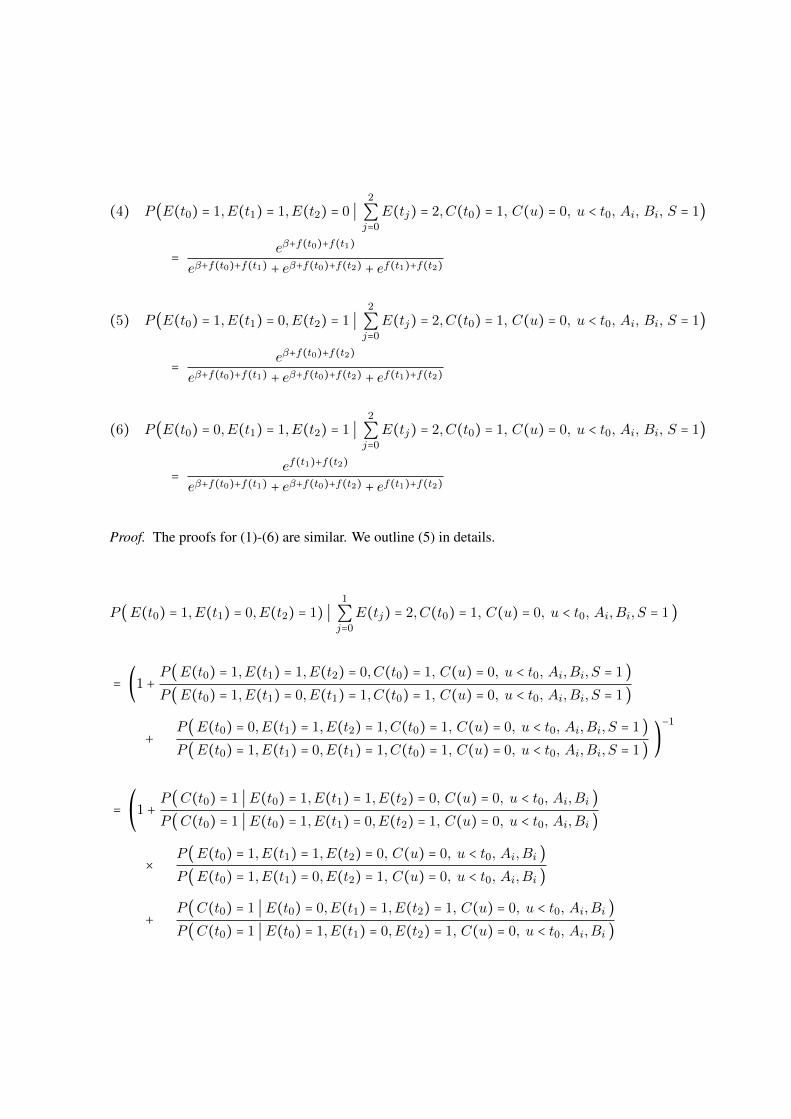
(4) P (E(t0) = 1,E(t1) = 1,E(t2) = 0 ∣2

∑j=0

E(tj) = 2,C(t0) = 1, C(u) = 0, u < t0, Ai, Bi, S = 1)

= eβ+f(t0)+f(t1)

eβ+f(t0)+f(t1) + eβ+f(t0)+f(t2) + ef(t1)+f(t2)

(5) P (E(t0) = 1,E(t1) = 0,E(t2) = 1 ∣2

∑j=0

E(tj) = 2,C(t0) = 1, C(u) = 0, u < t0, Ai, Bi, S = 1)

= eβ+f(t0)+f(t2)


(6) P (E(t0) = 0,E(t1) = 1,E(t2) = 1 ∣2

∑j=0

E(tj) = 2,C(t0) = 1, C(u) = 0, u < t0, Ai, Bi, S = 1)

= ef(t1)+f(t2)


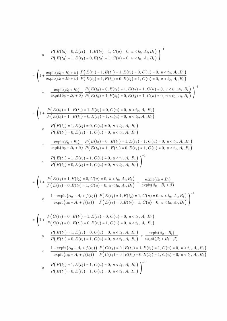
Proof. The proofs for (1)-(6) are similar. We outline (5) in details.

P (E(t0) = 1,E(t1) = 0,E(t2) = 1) ∣1

∑j=0

E(tj) = 2,C(t0) = 1, C(u) = 0, u < t0, Ai,Bi, S = 1 )

= (1 +P (E(t0) = 1,E(t1) = 1,E(t2) = 0,C(t0) = 1, C(u) = 0, u < t0, Ai,Bi, S = 1 )P (E(t0) = 1,E(t1) = 0,E(t1) = 1,C(t0) = 1, C(u) = 0, u < t0, Ai,Bi, S = 1 )

+P (E(t0) = 0,E(t1) = 1,E(t2) = 1,C(t0) = 1, C(u) = 0, u < t0, Ai,Bi, S = 1 )P (E(t0) = 1,E(t1) = 0,E(t1) = 1,C(t0) = 1, C(u) = 0, u < t0, Ai,Bi, S = 1 )

)−1

=⎛⎝

1 +P(C(t0) = 1 ∣ E(t0) = 1,E(t1) = 1,E(t2) = 0, C(u) = 0, u < t0, Ai,Bi )P (C(t0) = 1 ∣ E(t0) = 1,E(t1) = 0,E(t2) = 1, C(u) = 0, u < t0, Ai,Bi )

×P (E(t0) = 1,E(t1) = 1,E(t2) = 0, C(u) = 0, u < t0, Ai,Bi )P (E(t0) = 1,E(t1) = 0,E(t2) = 1, C(u) = 0, u < t0, Ai,Bi )

+P (C(t0) = 1 ∣ E(t0) = 0,E(t1) = 1,E(t2) = 1, C(u) = 0, u < t0, Ai,Bi )P (C(t0) = 1 ∣ E(t0) = 1,E(t1) = 0,E(t2) = 1, C(u) = 0, u < t0, Ai,Bi )

×P (E(t0) = 0,E(t1) = 1,E(t2) = 1, C(u) = 0, u < t0, Ai,Bi )P (E(t0) = 1,E(t1) = 0,E(t2) = 1, C(u) = 0, u < t0, Ai,Bi )

⎞⎠

−1

=⎛⎝

1 + expit(β0 +Bi + β)expit(β0 +Bi + β)

P (E(t0) = 1,E(t1) = 1,E(t2) = 0, C(u) = 0, u < t0, Ai,Bi )P (E(t0) = 1,E(t1) = 0,E(t2) = 1, C(u) = 0, u < t0, Ai,Bi )

+ expit(β0 +Bi)expit(β0 +Bi + β)

P (E(t0) = 0,E(t1) = 1,E(t2) = 1, C(u) = 0, u < t0, Ai,Bi )P (E(t0) = 1,E(t1) = 0,E(t2) = 1, C(u) = 0, u < t0, Ai,Bi )

⎞⎠

−1

=⎛⎝

1 +P (E(t0) = 1 ∣ E(t1) = 1,E(t2) = 0, C(u) = 0, u < t0, Ai,Bi )P (E(t0) = 1 ∣ E(t1) = 0,E(t2) = 1, C(u) = 0, u < t0, Ai,Bi )

×P (E(t1) = 1,E(t2) = 0, C(u) = 0, u < t0, Ai,Bi )P (E(t1) = 0,E(t2) = 1, C(u) = 0, u < t0, Ai,Bi )


P (E(t0) = 0 ∣ E(t1) = 1,E(t2) = 1, C(u) = 0, u < t0, Ai,Bi )P (E(t0) = 1 ∣ E(t1) = 0,E(t2) = 1, C(u) = 0, u < t0, Ai,Bi )


⎞⎠

−1

=⎛⎝

1 +P (E(t1) = 1,E(t2) = 0, C(u) = 0, u < t0, Ai,Bi )P (E(t1) = 0,E(t2) = 1, C(u) = 0, u < t0, Ai,Bi )


×1 − expit (α0 +Ai + f(t0))

expit (α0 +Ai + f(t0))P(E(t1) = 1,E(t2) = 1, C(u) = 0, u < t0, Ai,Bi )P(E(t1) = 0,E(t2) = 1, C(u) = 0, u < t0, Ai,Bi )

⎞⎠

−1

=⎛⎝

1 +P (C(t1) = 0 ∣ E(t1) = 1,E(t2) = 0, C(u) = 0, u < t1, Ai,Bi )P (C(t1) = 0 ∣ E(t1) = 0,E(t2) = 1, C(u) = 0, u < t1, Ai,Bi )



×1 − expit (α0 +Ai + f(t0))

expit (α0 +Ai + f(t0))P(C(t1) = 0 ∣ E(t1) = 1,E(t2) = 1, C(u) = 0, u < t1, Ai,Bi )P(C(t1) = 0 ∣ E(t1) = 0,E(t2) = 1, C(u) = 0, u < t1, Ai,Bi )


⎞⎠

−1

=⎛⎝

1 + 1 − expit(β0 +Bi + β)1 − expit(β0 +Bi)

P (E(t1) = 1,E(t2) = 0, C(u) = 0, u < t1, Ai,Bi )P (E(t1) = 0,E(t2) = 1, C(u) = 0, u < t1, Ai,Bi )



1 − expit(β0 +Bi + β)1 − expit(β0 +Bi)


⎞⎠

−1

=⎛⎝


P (E(t1) = 1 ∣ E(t2) = 0, C(u) = 0, u < t1, Ai,Bi )P (E(t1) = 0 ∣ E(t2) = 1, C(u) = 0, u < t1, Ai,Bi )

×P (E(t2) = 0, C(u) = 0, u < t1, Ai,Bi )P (E(t2) = 1, C(u) = 0, u < t1, Ai,Bi )

+ eβ0+Bi

eβ0+Bi+β1

eα0+Ai+f(t0)

P (E(t1) = 1 ∣ E(t2) = 1, C(u) = 0, u < t1, Ai,Bi )P (E(t1) = 0 ∣ E(t2) = 1, C(u) = 0, u < t1, Ai,Bi )

×P (E(t2) = 1, C(u) = 0, u < t1, Ai,Bi )P (E(t2) = 1, C(u) = 0, u < t1, Ai,Bi )

⎞⎠

−1

=⎛⎝


expit (α0 +Ai + f(t1))1 − expit (α0 +Ai + f(t1))

×P (C(t2) = 0 ∣ E(t2) = 0, C(u) = 0, u < t2, Ai,Bi )P (C(t2) = 0 ∣ E(t2) = 1, C(u) = 0, u < t2, Ai,Bi )

P (E(t2) = 0, C(u) = 0, u < t2, Ai,Bi )P (E(t2) = 1, C(u) = 0, u < t2, Ai,Bi )

+ e−β

eα0+Ai+f(t0)

expit (α0 +Ai + f(t1))1 − expit (α0 +Ai + f(t1))

⎞⎠

−1

=⎛⎝


eα0+Ai+f(t1) 1 − expit(β0 +Bi)1 − expit(β0 +Bi + β)

P (E(t2) = 0 ∣ C(u) = 0, u < t2, Ai,Bi )P (E(t2) = 1 ∣ C(u) = 0, u < t2, Ai,Bi )

+ e−β eα0+Ai+f(t1)

eα0+Ai+f(t0)⎞⎠

−1

=⎛⎝

1 + eα0+Ai+f(t1) 1 − expit (α0 +Ai + f(t2))expit (α0 +Ai + f(t2))

+ e−β eα0+Ai+f(t1)

eα0+Ai+f(t0)⎞⎠

−1

=⎛⎝

1 + ef(t1)−f(t2) + e−β+f(t1)−f(t0)⎞⎠

−1

eβ+f(t0)+f(t2)


3.5.2 Controls:

lemma 3.5.2.

(1) P (E(t0) = 1,E(t1) = 0,E(t2) = 0 ∣2

∑j=0

E(tj) = 1,C(t0) = 0, C(u) = 0, u < t0, Ai, Bi, S = 1 )

= ef(t0)

ef(t0) + ef(t1) + ef(t2)

(2) P (E(t0) = 0,E(t1) = 1,E(t2) = 0 ∣2

∑j=0

E(tj) = 1,C(t0) = 0, C(u) = 0, u < t0, Ai, Bi, S = 1 )

= ef(t1)

ef(t0) + ef(t1) + ef(t2)

(3) P (E(t0) = 0,E(t1) = 0,E(t2) = 1 ∣2

∑j=0

E(tj) = 1,C(t0) = 0, C(u) = 0, u < t0, Ai, Bi, S = 1 )

= ef(t2)

ef(t0) + ef(t1) + ef(t2)

(4) P (E(t0) = 1,E(t1) = 1,E(t2) = 0 ∣2

∑j=0

E(tj) = 2,C(t0) = 0, C(u) = 0, u < t0, Ai, Bi, S = 1 )

= ef(t0)+f(t1)

ef(t0)+f(t1) + ef(t0)+f(t2) + ef(t1)+f(t2)

(5) P (E(t0) = 1,E(t1) = 0,E(t2) = 1 ∣2

∑j=0

E(tj) = 2,C(t0) = 0, C(u) = 0, u < t0, Ai, Bi, S = 1 )

= ef(t0)+f(t2)


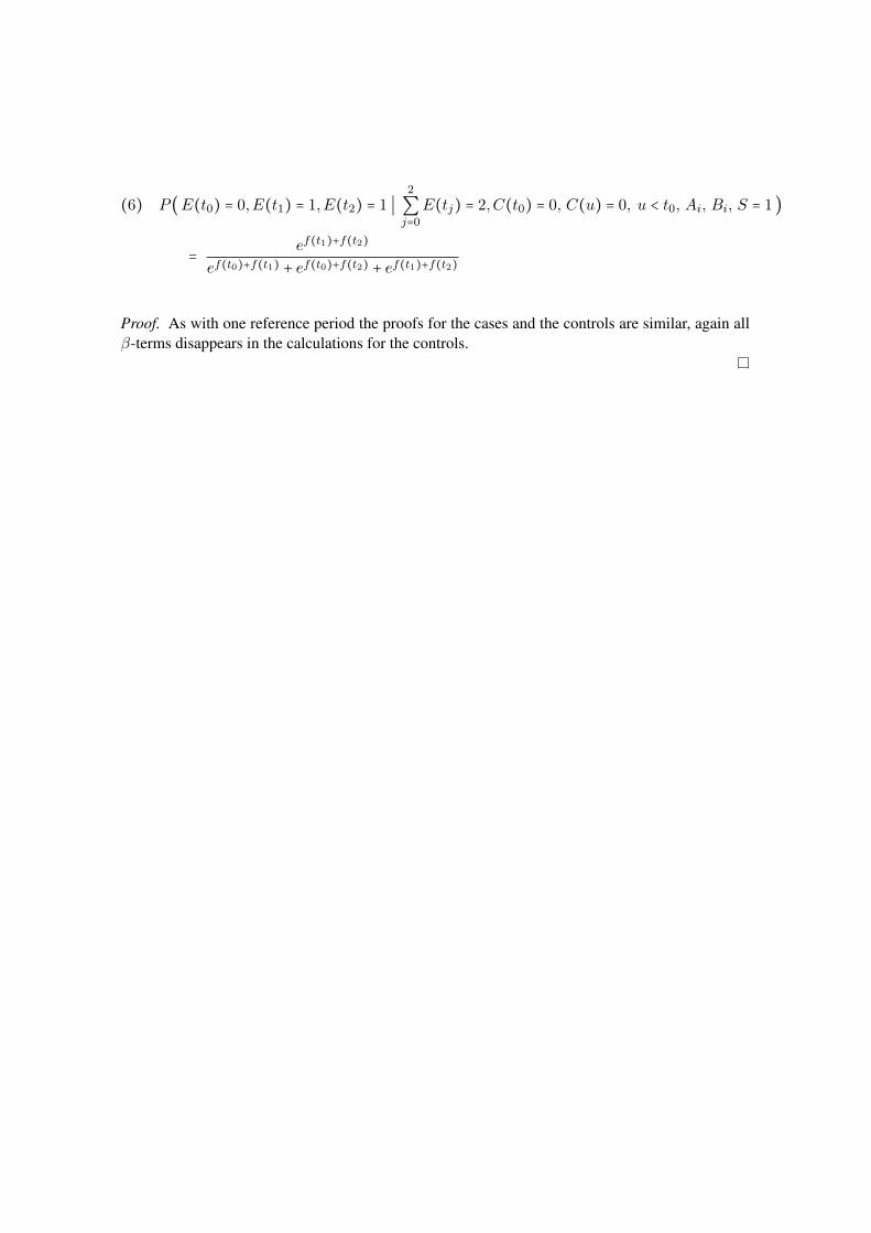
(6) P (E(t0) = 0,E(t1) = 1,E(t2) = 1 ∣2

∑j=0

E(tj) = 2,C(t0) = 0, C(u) = 0, u < t0, Ai, Bi, S = 1 )

= ef(t1)+f(t2)


Proof. As with one reference period the proofs for the cases and the controls are similar, again allβ-terms disappears in the calculations for the controls.

Research Reports available from Department of Biostatistics http://www.pubhealth.ku.dk/bs/publikationer ________________________________________________________________________________ Department of Biostatistics University of Copenhagen Øster Farimagsgade 5 P.O. Box 2099 1014 Copenhagen K Denmark 10/1 Andersen, P.K. & Skrondal, A. “Biological” interaction from a statistical point of view. 10/2 Rosthøj, S., Keiding, N., Schmiegelow, K. Application of History-Adjusted Marginal

Structural Models to Maintenance Therapy of Children with Acute Lymphoblastic Leukaemia.

10/3 Parner, E.T. & Andersen, P.K. Regression analysis of censored data using pseudo-

observations. 10/4 Nielsen, T. & Kreiner, S. Course Evaluation and Development: What can Learning Styles

Contribute? 10/5 Lange, T. & Hansen, J.V. Direct and Indirect Effects in a Survival Context. 10/6 Andersen, P.K. & Keiding, N. Interpretability and importance of functionals in

competing risks and multi-state models. 10/7 Gerds, T.A., Kattan, M.W., Schumacher, M. & Yu, C. Estimating a time-dependent

concordance index for survival prediction models with covariate dependent censoring. 10/8 Mogensen, U.B., Ishwaran, H. & Gerds, T.A. Evaluating random forests for survival

analysis using prediction error curves. 11/1 Kreiner, S. Is the foundation under PISA solid? A critical look at the scaling model

underlying international comparisons of student attainment. 11/2 Andersen, P.K. Competing risks in epidemiology: Possibilities and pitfalls. 11/3 Holst, K.K. Model diagnostics based on cumulative residuals: The R-package gof. 11/4 Holst, K.K. & Budtz-Jørgensen, E. Linear latent variable models: The lava-package.

11/5 Holst, K.K., Budtz-Jørgensen, E. & Knudsen, G.M. A latent variable model with mixed

binary and continuous response variables. 11/6 Cortese, G., Gerds, T.A., &Andersen, P.K. Comparison of prediction models for

competing risks with time-dependent covariates. 11/7 Scheike, T.H. & Sun, Y. On Cross-Odds Ratio for Multivariate Competing Risks Data. 11/8 Gerds, T.A., Scheike T.H. & Andersen P.K. Absolute risk regression for competing risks:

interpretation, link functions and prediction. 11/9 Scheike, T.H., Maiers, M.J., Rocha, V. & Zhang, M. Competing risks with missing

covariates: Effect of haplotypematch on hematopoietic cell transplant patients. 12/01 Keiding, N., Hansen, O.K.H., Sørensen, D.N. & Slama, R. The current duration approach

to estimating time to pregnancy. 12/02 Andersen, P.K. A note on the decomposition of number of life years lost according to

causes of death. 12/03 Martinussen, T. & Vansteelandt, S. A note on collapsibility and confounding bias in Cox

and Aalen regression models. 12/04 Martinussen, T. & Pipper, C.B. Estimation of Odds of Concordance based on the Aalen

additive model. 12/05 Martinussen, T. & Pipper, C.B. Estimation of Causal Odds of Concordance based on the

Aalen additive model. 12/06 Binder, N., Gerds, T.A. & Andersen, P.K. Pseudo-observations for competing risks with

covariate dependent censoring. 12/07 Keiding, N. & Clayton, D. Standardization and control for confounding in observational

studies: a historical perspective. 12/08 Hilden, J. & Gerds, T.A. Evaluating the impact of novel biomarkers: Do not rely on IDI

and NRI. 12/09 Gerster, M., Madsen, M. & Andersen, P.K. Matched Survival Data in a Co-twin Control

Design. 12/10 Scheike, T.H., Holst, K.K. & Hjelmborg, J.B. Estimating heritability for cause specific

mortality based on twin studies. 12/11 Jensen, A.K.G., Gerds, T.A., Weeke, P., Torp-Pedersen C. & Andersen, P.K. A note on the

validity of the case-time-control design for autocorrelated exposure histories.

Department of Biostatistics University of Copenhagen

Documents

Transcript of Department of Biostatistics University of Copenhagen