DEPARTMENT OF ANTHROPOLOGY AND SOCIOLOGY

HILBERT’S FOURTH PROBLEM IN TWO DIMENSIONS I

J.C. ALVAREZ PAIVA

Abstract. Hilbert’s fourth problems asks to construct and study thegeometries in which the straight line segment is the shortest connectionbetween two points. In this paper the reader shall find an elementaryintroduction to the problem and its solutions in dimension two by Buse-mann, Pogorelov, and Ambartzumian. The relationship between inte-gral geometry and inverse problems in variational calculus is emphasized.

Contents

1. Introduction 12. Basic definitions and interpretations of the problem 23. Minkowski planes 64. Hilbert geometries 95. The Crofton formula 106. Busemann’s construction of projective metrics 137. Ambartzumian’s construction 148. Variational interpretation of Hilbert’s fourth problem 159. Analytic solution of Hilbert’s fourth problem 1710. A glimpse ahead 20References 21

1. Introduction

Hilbert’s list of problems, read at the International Congress of Mathe-maticians in 1900, is perhaps one of the most influential documents in thehistory of mathematics. The twenty-three problems in this list have beenthe subject of numerous investigations for the last hundred years and con-tinue to yield much beautiful mathematics. Even when one of Hilbert’sproblems has been solved in its original formulation, its variations and thedevelopments arising from its solution continue to pique the curiosity ofmathematicians. One example is Hilbert’s third problem on the decompo-sition of polyhedra (see chapter seven in [1]). This problem was solved byM. Dehn ([23]) just two years after Hilbert’s address, but the concepts heintroduced have evolved in different directions. For instance, the theory of

Key words and phrases. Integral geometry, Crofton formula, Hilbert’s fourth problem,Minkowski spaces, cosine transform.

1

2 J.C. ALVAREZ PAIVA

valuations, a central part of modern convex geometry, is a direct descendentof Dehn’s solution.

In posing his problems, Hilbert did not shy away from vague statementswhich would be subject to interpretation. Problem six on the mathematicaltreatment of the axioms of physics is perhaps the prime example of this.Hilbert’s fourth problem, the subject of this note, is another.

In its original formulation, Hilbert’s fourth problem asks to constructand study the geometries in which the straight line segment is the shortestconnection between two points. The original wording (see [25]) makes onethink the problem is part of Hilbert’s project to study the foundations ofgeometry. However, the different modern approaches make it clear that theproblem is at the basis of integral geometry, inverse problems in the calculusof variations, and Finsler geometry.

In this paper the reader will find various approaches to the solution ofHilbert’s fourth problem in two dimensions. We will start with the examplesgiven by Minkowski and Hilbert of metrics where the shortest connectionbetween two points is a line segment, and proceed to the constructions ofBusemann and Ambartzumian which together give the most elegant andnatural solution to the problem. Later, we will cover Pogorelov’s approachusing Hamel’s equations and the cosine transform. A second paper shalltreat the subject from the symplectic viewpoint.

An effort has been made to make the paper partly accessible to undergrad-uate students and mathematically minded readers from other disciplines.The material is presented as a collection of exercises some of which point atextensions or digressions of the ideas which led to the solution of Hilbert’sfourth problem in two dimensions. From the author’s viewpoint, Hilbert’sfourth problem is simply an axis around which revolve two fruitful lines ofresearch: the relation between integral geometry and variational calculusand the relation between metric and symplectic geometry. The advancedreader is asked to keep these two themes in mind as he/she reads the paper.

For more information on Hilbert’s problems the reader is referred to thetwo volumes “Mathematical developments arising from Hilbert problems”,Proceedings of Symposia in Pure Math. Vol. XXVII Part 1, F. Browder(Ed.), AMS Rhode Island, 1974, and to the recently published “The HonorsClass: Hilbert’s problems and their solvers” by Benjamin Yandell, A KPeters, Ltd, 2001.

2. Basic definitions and interpretations of the problem

Most interpretations of Hilbert’s fourth problem revolve around the notionof distance or metric. To find all the possible definitions of distance on theplane for which the shortest path between two given points is the line segmentthat joins them is a clear and attractive formulation. Of course, our usualnotion of distance in two dimensions, borrowed from Euclidean geometry,satisfies this property and we may wonder if there is any other that does. In

HILBERT’S FOURTH PROBLEM IN TWO DIMENSIONS I 3

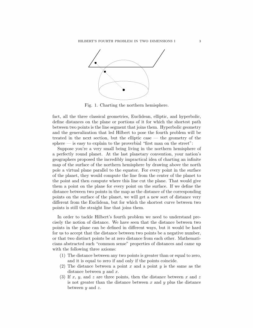
Fig. 1. Charting the northern hemisphere.

fact, all the three classical geometries, Euclidean, elliptic, and hyperbolic,define distances on the plane or portions of it for which the shortest pathbetween two points is the line segment that joins them. Hyperbolic geometryand the generalization that led Hilbert to pose the fourth problem will betreated in the next section, but the elliptic case — the geometry of thesphere — is easy to explain to the proverbial “first man on the street”:

Suppose you’re a very small being living in the northern hemisphere ofa perfectly round planet. At the last planetary convention, your nation’sgeographers proposed the incredibly impractical idea of charting an infinitemap of the surface of the northern hemisphere by drawing above the northpole a virtual plane parallel to the equator. For every point in the surfaceof the planet, they would compute the line from the center of the planet tothe point and then compute where this line cut the plane. That would givethem a point on the plane for every point on the surface. If we define thedistance between two points in the map as the distance of the correspondingpoints on the surface of the planet, we will get a new sort of distance verydifferent from the Euclidean, but for which the shortest curve between twopoints is still the straight line that joins them.

In order to tackle Hilbert’s fourth problem we need to understand pre-cisely the notion of distance. We have seen that the distance between twopoints in the plane can be defined in different ways, but it would be hardfor us to accept that the distance between two points be a negative number,or that two distinct points be at zero distance from each other. Mathemati-cians abstracted such “common sense” properties of distances and came upwith the following three axioms:

(1) The distance between any two points is greater than or equal to zero,and it is equal to zero if and only if the points coincide.

(2) The distance between a point x and a point y is the same as thedistance between y and x.

(3) If x, y, and z are three points, then the distance between x and zis not greater than the distance between x and y plus the distancebetween y and z.


Any measurement that assigns to any two points a number and that sat-isfies the three properties above is deemed to be a possible way of measuringdistances. It is sometimes convenient to admit that two points are at infinitedistance from each other. The definition that you would find in a textbookruns as follows:

Definition 2.1. A metric space is a pair (X, d), where X is a set and thedistance function, or metric,

d : X ×X −→ R ∪ {∞}satisfies following properties:

• Positivity: d(x, y) ≥ 0, and d(x, y) = 0 if and only if x = y.• Symmetry: d(x, y) = d(y, x).• Triangle inequality: d(x, z) ≤ d(x, y) + d(y, z).

A very simple example of a metric space with a surprising connection toHilbert’s fourth problem is constructed as follows:

Take S to be the collection of all subsets of {1, . . . , n}. Some of theelements of S are the empty set, {1}, {2, 3}, and {1, . . . , n}. If x and y arein S define d(x, y) as the number of elements in x which are not in y plusthe number of elements of y that are not in x. For example,

d({1, 2}, {2, 5, 6}) = 3.

Exercise 2.1. Show that (S, d) is a metric space. Moreover, S satisfiesthe following stronger version of the triangle inequality: if x1, . . . , xk areelements of S and b1, . . . , bk are integer numbers that add up to 1, then

k∑

i,j=1

d(xi, xj)bibj ≤ 0.

For k = 3 the above property is just a fancy way to rewrite the triangleinequality. When a metric space satisfies this property for any positiveinteger k, it is called hypermetric. Remarkably, all the solutions to Hilbert’sfourth problem in dimension two are hypermetric. This was first remarkedby R. Alexander in [2].

Exercise 2.2. Define the distance between two points (x, y, z) and (x′, y′, z′)in three-dimensional space as the biggest of the three numbers |x−x′|, |y−y′|,and |z − z′|. Show that this distance is not hypermetric.

Now that we understand the freedom we have in the choice of a distancefunction, it remains to makes sense of the term “the shortest path” thatappears in our metric interpretation of Hilbert’s fourth problem. For thatwe must understand how to compute the length of a path in a metric space.

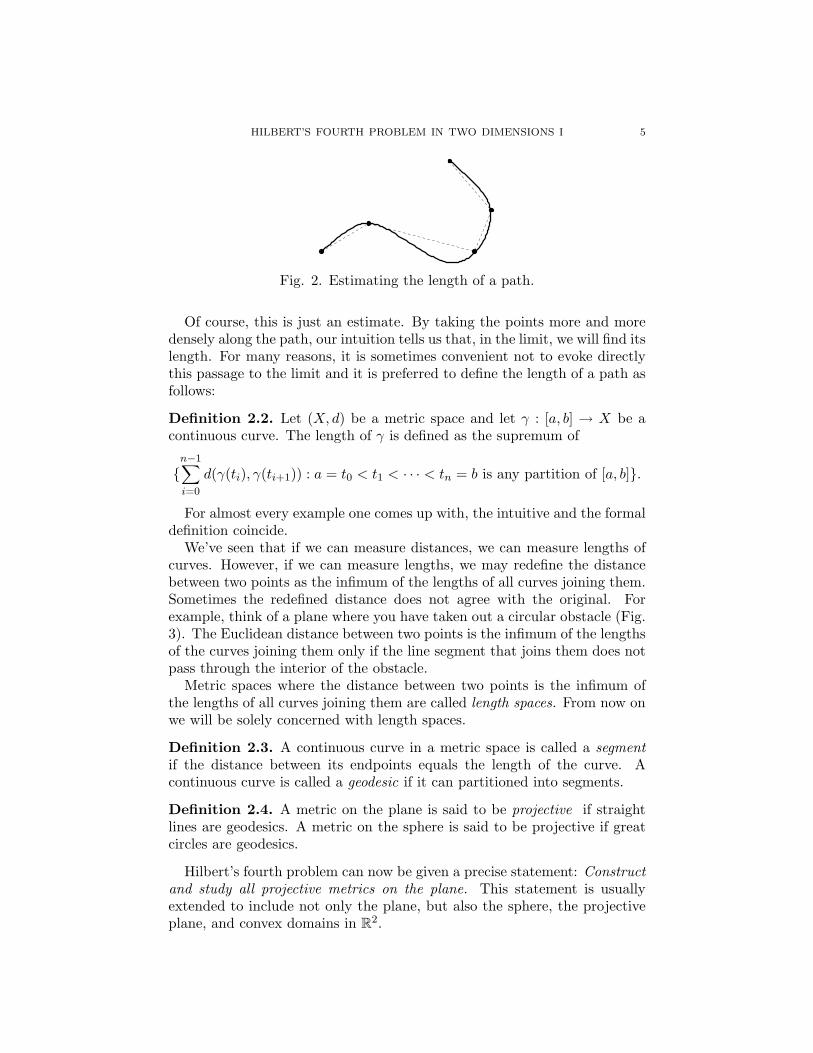
If all we know is to measure distances between pairs of points, a naturalway to estimate the length of a path is to mark a number of points on it,measure the distances between consecutive points, and add them up.


Fig. 2. Estimating the length of a path.

Of course, this is just an estimate. By taking the points more and moredensely along the path, our intuition tells us that, in the limit, we will find itslength. For many reasons, it is sometimes convenient not to evoke directlythis passage to the limit and it is preferred to define the length of a path asfollows:

Definition 2.2. Let (X, d) be a metric space and let γ : [a, b] → X be acontinuous curve. The length of γ is defined as the supremum of

{n−1∑

i=0

d(γ(ti), γ(ti+1)) : a = t0 < t1 < · · · < tn = b is any partition of [a, b]}.

For almost every example one comes up with, the intuitive and the formaldefinition coincide.

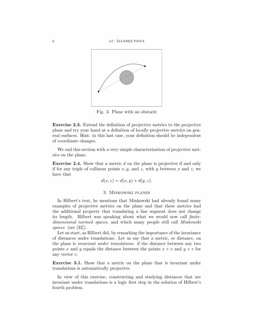
We’ve seen that if we can measure distances, we can measure lengths ofcurves. However, if we can measure lengths, we may redefine the distancebetween two points as the infimum of the lengths of all curves joining them.Sometimes the redefined distance does not agree with the original. Forexample, think of a plane where you have taken out a circular obstacle (Fig.3). The Euclidean distance between two points is the infimum of the lengthsof the curves joining them only if the line segment that joins them does notpass through the interior of the obstacle.

Metric spaces where the distance between two points is the infimum ofthe lengths of all curves joining them are called length spaces. From now onwe will be solely concerned with length spaces.

Definition 2.3. A continuous curve in a metric space is called a segmentif the distance between its endpoints equals the length of the curve. Acontinuous curve is called a geodesic if it can partitioned into segments.

Definition 2.4. A metric on the plane is said to be projective if straightlines are geodesics. A metric on the sphere is said to be projective if greatcircles are geodesics.

Hilbert’s fourth problem can now be given a precise statement: Constructand study all projective metrics on the plane. This statement is usuallyextended to include not only the plane, but also the sphere, the projectiveplane, and convex domains in R2.


Fig. 3. Plane with an obstacle

Exercise 2.3. Extend the definition of projective metrics to the projectiveplane and try your hand at a definition of locally projective metrics on gen-eral surfaces. Hint: in this last case, your definition should be independentof coordinate changes.

We end this section with a very simple characterization of projective met-rics on the plane.

Exercise 2.4. Show that a metric d on the plane is projective if and onlyif for any triple of collinear points x, y, and z, with y between x and z, wehave that

d(x, z) = d(x, y) + d(y, z).

3. Minkowski planes

In Hilbert’s text, he mentions that Minkowski had already found manyexamples of projective metrics on the plane and that these metrics hadthe additional property that translating a line segment does not changeits length. Hilbert was speaking about what we would now call finite-dimensional normed spaces, and which many people still call Minkowskispaces (see [32]).

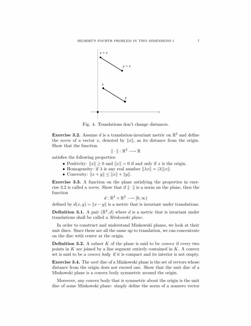
Let us start, as Hilbert did, by remarking the importance of the invarianceof distances under translations. Let us say that a metric, or distance, onthe plane is invariant under translations if the distance between any twopoints x and y equals the distance between the points x + v and y + v forany vector v.

Exercise 3.1. Show that a metric on the plane that is invariant undertranslations is automatically projective.

In view of this exercise, constructing and studying distances that areinvariant under translations is a logic first step in the solution of Hilbert’sfourth problem.


x

y

x + v

y + v

Fig. 4. Translations don’t change distances.

Exercise 3.2. Assume d is a translation-invariant metric on R2 and definethe norm of a vector x, denoted by ‖x‖, as its distance from the origin.Show that the function

‖ · ‖ : R2 −→ Rsatisfies the following properties:

• Positivity: ‖x‖ ≥ 0 and ‖x‖ = 0 if and only if x is the origin.• Homogeneity: if λ is any real number ‖λx‖ = |λ|‖x‖.• Convexity: ‖x + y‖ ≤ ‖x‖+ ‖y‖.

Exercise 3.3. A function on the plane satisfying the properties in exer-cise 3.2 is called a norm. Show that if ‖ · ‖ is a norm on the plane, then thefunction

d : R2 × R2 −→ [0,∞)defined by d(x, y) = ‖x− y‖ is a metric that is invariant under translations.

Definition 3.1. A pair (R2, d) where d is a metric that is invariant undertranslations shall be called a Minkowski plane.

In order to construct and understand Minkowski planes, we look at theirunit discs. Since these are all the same up to translation, we can concentrateon the disc with center at the origin.

Definition 3.2. A subset K of the plane is said to be convex if every twopoints in K are joined by a line segment entirely contained in K. A convexset is said to be a convex body if it is compact and its interior is not empty.

Exercise 3.4. The unit disc of a Minkowski plane is the set of vectors whosedistance from the origin does not exceed one. Show that the unit disc of aMinkowski plane is a convex body symmetric around the origin.

Moreover, any convex body that is symmetric about the origin is the unitdisc of some Minkowski plane: simply define the norm of a nonzero vector


(x,y)

(x’,y’)(x,y)

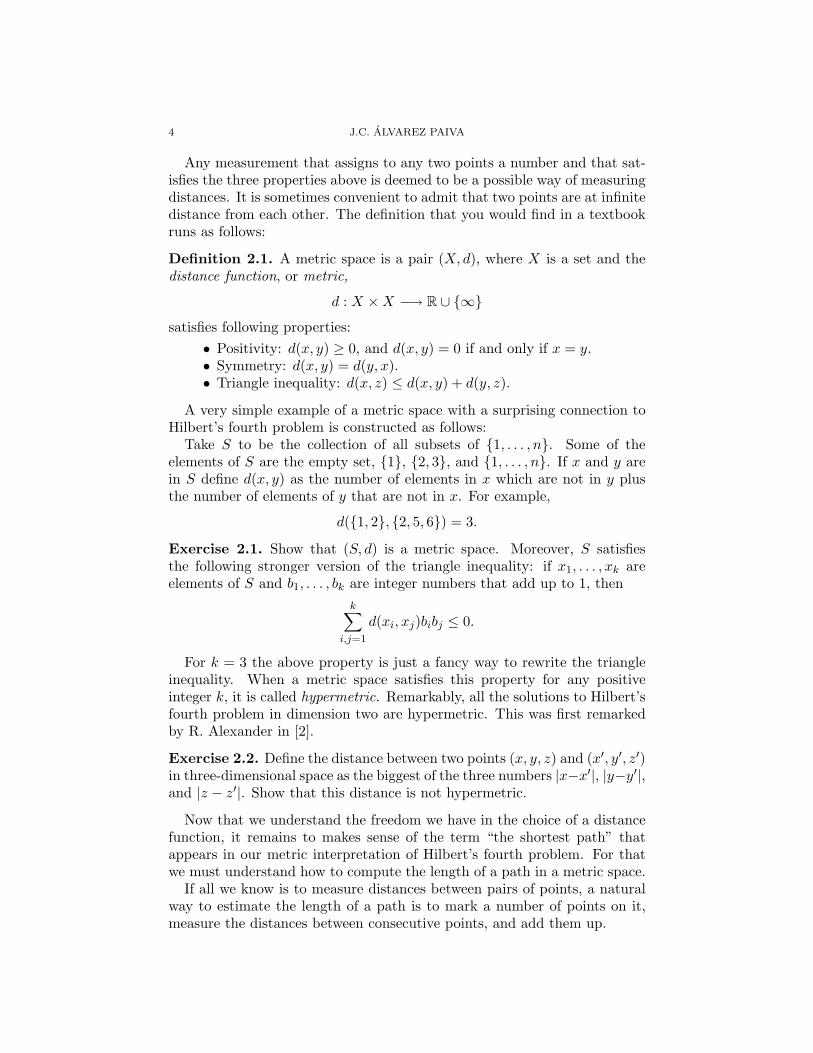
(x’,y’)

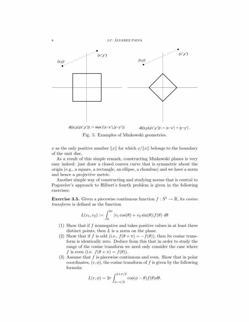
d((x,y),(x’,y’)) := max {|x−x’|,|y−y’|}. d((x,y),(x’,y’)) := |x−x’| + |y−y’| .

Fig. 5. Examples of Minkowski geometries.

x as the only positive number ‖x‖ for which x/‖x‖ belongs to the boundaryof the unit disc.

As a result of this simple remark, constructing Minkowski planes is veryeasy indeed: just draw a closed convex curve that is symmetric about theorigin (e.g., a square, a rectangle, an ellipse, a rhombus) and we have a normand hence a projective metric.

Another simple way of constructing and studying norms that is central toPogorelov’s approach to Hilbert’s fourth problem is given in the followingexercises:

Exercise 3.5. Given a piecewise continuous function f : S1 → R, its cosinetransform is defined as the function

L(v1, v2) :=∫ 2π

0|v1 cos(θ) + v2 sin(θ)|f(θ) dθ

(1) Show that if f nonnegative and takes positive values in at least threedistinct points, then L is a norm on the plane.

(2) Show that if f is odd (i.e., f(θ + π) = −f(θ)), then its cosine trans-form is identically zero. Deduce from this that in order to study therange of the cosine transform we need only consider the case wheref is even (i.e. f(θ + π) = f(θ)).

(3) Assume that f is piecewise continuous and even. Show that in polarcoordinates, (r, φ), the cosine transform of f is given by the followingformula:

L(r, φ) = 2r∫ φ+π/2

φ−π/2cos(φ− θ)f(θ)dθ.


(4) With f and L as in the previous item, show that

f(φ + π/2) :=14r

(L(r, φ) +

∂2L

∂φ2(r, φ)

).

Exercise 3.6. Show that if f is a smooth positive function on the circle andL is its cosine transform in cartesian coordinates (v1, v2), then the matrixformed by the second partial derivatives of L2 is positive definite. Geomet-rically, this means that the unit circle of the Minkowski plane (R2, L) issmooth and has positive curvature everywhere.

A norm L : R2 → [0,∞) that is smooth outside the origin and such thatthe matrix formed by the second partial derivatives of L2 is positive definiteis said to satisfy the Legendre condition. The previous exercise shows thatthe cosine transform of a smooth positive function on the circle is a such anorm, while item (4) on exercise 3.5 shows that every norm satisfying theLegendre condition is the cosine transform of a smooth positive function onthe circle. Summarizing, we have the following result:

Theorem 3.1 (Blaschke, [17]). The cosine transform establishes a bijectionbetween the set of smooth, even, positive functions on the circle and normson the plane that satisfy the Legendre condition.

4. Hilbert geometries

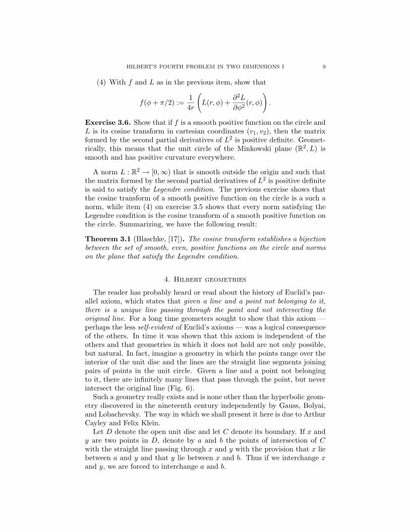
The reader has probably heard or read about the history of Euclid’s par-allel axiom, which states that given a line and a point not belonging to it,there is a unique line passing through the point and not intersecting theoriginal line. For a long time geometers sought to show that this axiom —perhaps the less self-evident of Euclid’s axioms — was a logical consequenceof the others. In time it was shown that this axiom is independent of theothers and that geometries in which it does not hold are not only possible,but natural. In fact, imagine a geometry in which the points range over theinterior of the unit disc and the lines are the straight line segments joiningpairs of points in the unit circle. Given a line and a point not belongingto it, there are infinitely many lines that pass through the point, but neverintersect the original line (Fig. 6).

Such a geometry really exists and is none other than the hyperbolic geom-etry discovered in the nineteenth century independently by Gauss, Bolyai,and Lobachevsky. The way in which we shall present it here is due to ArthurCayley and Felix Klein.

Let D denote the open unit disc and let C denote its boundary. If x andy are two points in D, denote by a and b the points of intersection of Cwith the straight line passing through x and y with the provision that x liebetween a and y and that y lie between x and b. Thus if we interchange xand y, we are forced to interchange a and b.


Fig. 6. Infinitely many parallel lines passing through the same point.

The hyperbolic distance between x and y is defined by the equation

d(x, y) :=12

ln(‖y − a‖‖x− a‖

‖x− b‖‖y − b‖

).

Exercise 4.1. Show that the function d satisfies the three following prop-erties:

(1) Positivity: d(x, y) ≥ 0, and d(x, y) = 0 if and only if x = y.(2) Symmetry: d(x, y) = d(y, x).(3) If x, y, and z are three aligned points in D such that y lies between

x and z. Show that d(x, z) = d(x, y) + d(y, z).

The proof of the triangle inequality for d is somewhat more elaborate, butit only makes use of elementary projective geometry (see chapter 5 in [6]).Part (3) of exercise 4.1 shows that this metric is projective.

In [26], Hilbert shows that it is possible to replace the open unit disc Din the construction above by the interior of any convex body in the planewithout changing the fact that d is a projective metric.

Hilbert geometries, as these metric spaces are called, are a natural gen-eralization of hyperbolic geometry and furnish us with a second large classof examples of projective metrics. Recently, much progress has been madein the understanding of the Hilbert geometries (see, for example, [30] and[27]).

5. The Crofton formula

The key to the solution of many problems in geometry is simply a changeof viewpoint. So far we have concentrated on points and the distancesbetween them. Hilbert’s fourth problem asks for those metrics for which thegeodesics are straight lines, so perhaps the best strategy is to replace thepoint for the straight line as the fundamental object of our investigations.

We shall take as departing point the following naive question: what wouldEuclidean geometry look like if we take the straight line instead of the pointas our basic geometric entity?


l

z = 1

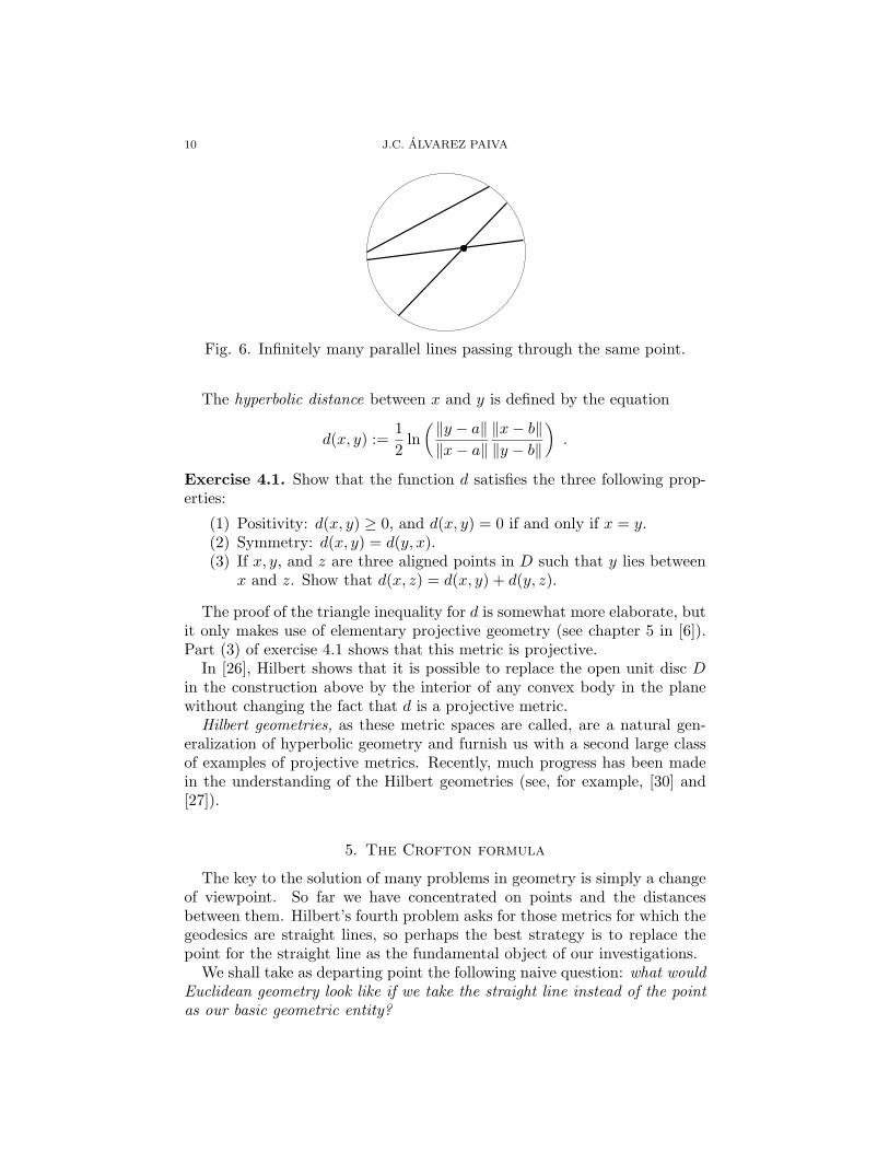
Fig. 7. The cylinder as the space of oriented lines.

The space of oriented lines. We may identify the space of orientedstraight lines on the plane with the right circular cylinder x2 + y2 = 1 inthree-dimensional space by means of the following construction:

An oriented line ` lying on the plane z = 0 in three-dimensional space isuniquely determined by the unit vector q defining its direction, and by thevector v representing the point on the line that is closest to the origin. Themap ` 7→ q + q × v identifies the space of oriented lines on the plane z = 0with the cylinder x2 + y2 = 1.

Another, more geometric, correspondence may be given if we consider notthe plane z = 0, but the plane z = 1. In fact, any line ` on z = 1 is theintersection of this plane with some plane Π through the origin. Using theorientation on the line, we may determine which side of the plane Π is upand which is down: if you’re walking head up along the line in the senseof its orientation, then the origin of R3 should be to your left. In order toidentify ` with a point on the cylinder, simply trace an orthogonal ray upfrom Π at the origin and mark where it intersects the cylinder (Fig. 7).

Exercise 5.1. Discover the simple relationship between both identificationsof the space of oriented lines with the right circular cylinder. In the rest ofthe paper, we use the first of these identifications.

The aim of the following exercises is to get an intuitive feeling for thecorrespondence between points on the cylinder x2 + y2 = 1, and henceforthdenoted by C, and oriented lines on the plane. This intuition is crucial forthe understanding of the rest of the paper. Please take ten minutes to dothem on your own and then come back to the paper.

Exercise 5.2. Draw the portion of the cylinder that corresponds to alloriented lines passing through

(1) a point,(2) a line segment,


(3) the unit disc centered at the origin,(4) two sides of a given triangle.

Exercise 5.3. The cylinder C admits the parameterization

(p, θ) 7−→ (cos(θ), sin(θ), p),

where 0 ≤ θ < 2π, and p is any real number. Draw the region in the(p, θ)-plane that corresponds to all oriented lines passing through

(1) a point,(2) a line segment,(3) the unit disc centered at the origin,(4) two sides of a given triangle.

Euclidean transformations preserve areas. A rigid motion, or Eu-clidean transformation, on the plane is a transformation from the planeonto itself that preserves distances. It is not too hard to see that thesetransformations are composed of translations and rotations, and that theysend oriented straight lines to oriented straight lines. We have then thatEuclidean transformations of the plane induce a class of transformations onthe space of oriented lines C. Let us now understand this class of transfor-mations and discover what geometric properties they may have.

Exercise 5.4. Parameterize each point in the cylinder C by its height p andthe angle, θ, that its projection makes with the positive x-axis (i.e., a pointin C has coordinates (cos(θ), sin(θ), p)).

(1) Show that rotating the oriented line represented by (p, θ) counter-clockwise by an angle φ around the origin results in the oriented linerepresented by (p, θ + φ).

(2) Show that translating the oriented line represented by (p, θ) by avector (x, y) results in the oriented line represented by (p+x cos(θ)+y sin(θ), θ).

Exercise 5.5. Show that the area of the portion of the right circular cylinderx2 + y2 = 1 given by all points with coordinates (cos(θ), sin(θ), p), where(p, θ) ranges over some region R is just∫

Rdpdθ.

Conclude that the area of a region in the space of oriented lines is invariantunder the action of Euclidean transformations.

Defining distance in terms of areas. So far our project of studying Eu-clidean geometry by taking the line instead of the point as basic geometricentity has led us to consider the space of oriented lines, to study the actionof Euclidean transformations on this space, and to the remarkable fact thatthese transformations preserve areas. However, in order to gain full under-standing, we must try to reconstruct the Euclidean distance on the planeby using the geometry on the space of lines.


Exercise 5.6. Use exercises 5.3 and 5.5 to show that the area in C of theregion representing the set of all oriented lines passing through a line segmentequals four times its length.

Exercise 5.7. Use exercise 5.6 to show that the length of a polygonal curveγ in the plane is given by the following integral over the space of orientedlines C

14

∫

`∈C#(` ∩ γ) dA,

where dA is the element of area on the cylinder.

By approximating rectifiable curves by polygonal ones, the previous exer-cises furnishes us with a proof of the Crofton formula in Euclidean geometry.

Theorem 5.1 (Crofton formula). If γ ⊂ R2 is a rectifiable curve and dA isthe standard area element on the cylinder C, then

length(γ) =14

∫

`∈C#(` ∩ γ) dA.

Exercise 5.8. Use the Crofton formula to give an easy proof of the follow-ing, apparently obvious, fact: if a convex body K ⊂ R2 contains a secondconvex body L, then the perimeter of K is greater than or equal to theperimeter of L with equality holding if and only if K = L.

6. Busemann’s construction of projective metrics

The simple remark that underlies the solution of Hilbert’s fourth problemis that the Crofton formula implies that straight lines are geodesics. In fact,if γ is a rectifiable curve on the plane joining the points x and y, then anyoriented line intersecting the line segment that joins them must intersect γ.Applying Crofton’s formula, we see that the length of γ is greater than orequal to that of the line segment joining x and y. The independence of thisargument on the special nature of the area element on C suggests replacingdA by other ways of measuring areas on the space of oriented lines.

Any continuous area element on the space of oriented lines, C, has theform fdA, where f is some positive, continuous function on C. Let us agreeto call the area, measured with fdA, of a region R in C the f-area of R .

If f is a positive, continuous function of C, define a metric on the plane bysetting the distance between any two points as one fourth times the f -areaof the set of all oriented lines that intersect the segment that joins them.

Exercise 6.1. Show that the construction above does indeed define a dis-tance function on the plane and that this distance is necessarily projective.This is Busemann’s construction of projective metrics.

The same arguments in your solution of exercise 5.7 show that Crofton’sformula holds for the metrics defined by Busemann’s construction. In fact,these metrics were defined so that Crofton’s formula be a tautology.


Exercise 6.2. Let f be a positive, continuous function on the space of ori-ented lines that depends only on the direction of the oriented line. Show thatBusemann’s construction yields a translation invariant metric, and hence anorm, on the plane.

A metric d on the plane is said to be periodic if there exists two linearlyindependent vectors v and w such that translation by any vector of the formmv + nv, m,n any integers, preserves distances. In general, periodic met-rics are not invariant under all translations, however we have the followingexercise:

Exercise 6.3. Suppose a metric arising from Busemann’s construction isperiodic. Show that it is invariant under translations and, hence, comesfrom a norm on the plane.

7. Ambartzumian’s construction

Busemann’s construction shows that to any continuous way of measur-ing areas in the space of oriented lines we can associate a continuous wayof measuring distances in the plane such that geodesics are straight lines.The natural question now is whether all projective metrics can be obtainedfrom Busemann’s construction. In [13], Ambartzumian gives a beautiful andsimple construction that answers this question affirmatively.

We start by remarking a nearly obvious property of Busemann’s construc-tion.

Exercise 7.1. Let fdA be a continuous element of area in the space oforiented lines and let d be the projective metric on the plane obtained fromfdA using Busemann’s construction. Show that the f -area of the set of alloriented lines passing through both the xy and yz sides of a triangle xyz isequal to two times the quantity d(x, y) + d(y, z)− d(x, z).

This simple remark is the basis of Ambartzumian’s construction: if dis a continuous distance function on the plane that satisfies the projectivecondition d(a, b)+d(b, c) = d(a, c) whenever b lies in the line segment joininga and c, we define the area of the set of all lines passing through boththe xy and yz sides of a triangle xyz as two times the quantity d(x, y) +d(y, z)− d(x, z). The projective condition guarantees that this set functionis additive, and the family of sets on which it is defined is sufficiently large sothat the set function admits a unique extension to a continuous measure onthe set of oriented lines provided we specify that this measure be invariantunder the map that changes the orientation of the lines. While the detailsin the proofs of these statements are beyond the scope of this article, theexercises below should give the reader a good sense of why they are true.

We start by describing the set of all oriented lines passing through twosides of a triangle in the plane as a subset of the cylinder. Of course, theconscientious reader has already done this exercise in section 5.


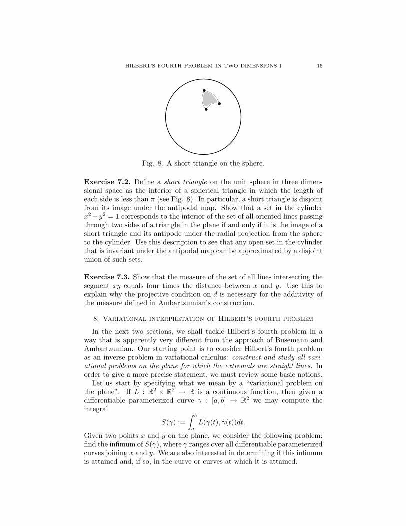
Fig. 8. A short triangle on the sphere.

Exercise 7.2. Define a short triangle on the unit sphere in three dimen-sional space as the interior of a spherical triangle in which the length ofeach side is less than π (see Fig. 8). In particular, a short triangle is disjointfrom its image under the antipodal map. Show that a set in the cylinderx2 +y2 = 1 corresponds to the interior of the set of all oriented lines passingthrough two sides of a triangle in the plane if and only if it is the image of ashort triangle and its antipode under the radial projection from the sphereto the cylinder. Use this description to see that any open set in the cylinderthat is invariant under the antipodal map can be approximated by a disjointunion of such sets.

Exercise 7.3. Show that the measure of the set of all lines intersecting thesegment xy equals four times the distance between x and y. Use this toexplain why the projective condition on d is necessary for the additivity ofthe measure defined in Ambartzumian’s construction.

8. Variational interpretation of Hilbert’s fourth problem

In the next two sections, we shall tackle Hilbert’s fourth problem in away that is apparently very different from the approach of Busemann andAmbartzumian. Our starting point is to consider Hilbert’s fourth problemas an inverse problem in variational calculus: construct and study all vari-ational problems on the plane for which the extremals are straight lines. Inorder to give a more precise statement, we must review some basic notions.

Let us start by specifying what we mean by a “variational problem onthe plane”. If L : R2 × R2 → R is a continuous function, then given adifferentiable parameterized curve γ : [a, b] → R2 we may compute theintegral

S(γ) :=∫ b

aL(γ(t), γ(t))dt.

Given two points x and y on the plane, we consider the following problem:find the infimum of S(γ), where γ ranges over all differentiable parameterizedcurves joining x and y. We are also interested in determining if this infimumis attained and, if so, in the curve or curves at which it is attained.


The integrand to keep in mind is the function

L0(x1, x2, v1, v2) :=√

v21 + v2

1 ,

which yields the variational problem of finding the shortest curve betweentwo points in the Euclidean plane. This suggests taking an arbitrary functionL(x1, x2, v1, v2) and defining the length of a parameterized curve γ : [a, b] →R2 as the integral

S(γ) :=∫ b

aL(γ(t), γ(t))dt.

Two basic properties of length that we would like our definition to satisfyare

(1) The length of any differentiable curve γ is a nonnegative number andit is zero if and only if the curve is constant (i.e., it is a point).

(2) The length of a curve does not depend on the way we traverse it.In other words, length should be invariant under changes of param-eterizations.

Exercise 8.1. Let L : R2 × R2 → R be a continuous function and use itto define a “length” for differentiable parameterized curves in the mannerdescribed above.

• Show that property (1) holds if and only if L(x1, x2, v1, v2) is non-negative and it is zero if and only if v1 and v2 are both equal tozero.

• Show that property (2) holds if and only if L is homogeneous of orderone in the last two coordinates: L(x1, x2, λv1, λv2) = |λ|L(x1, x2, v1, v2).

The third requirement we shall make of our definition of length is moresubtle: using lengths, we may define the distance between two points asthe infimum of the lengths of all differentiable curves joining them. Wemay then use this definition of distance to redefine the lengths of curves aswas done in section 2. The two ways of measuring lengths may not agree.Indeed, Busemann and Mayer proved in [22] that they agree if and only ifthe function L is convex in the last two variables:

L(x1, x2, v1 + w1, v2 + w2) ≤ L(x1, x2, v1, v2) + L(x1, x2, w1, w2).

We may summarize all three requirements on the function L by sayingthat for every point (x1, x2) on the plane the function (v1, v2) 7→ L(x1, x2, v1, v2)is a norm.

Exercise 8.2. Let L : R2 ×R2 → R be a continuous function such that forevery point (x1, x2) on the plane the function (v1, v2) 7→ L(x1, x2, v1, v2) is anorm. Define the length of a differentiable parameterized curve γ : [a, b] →R2 as the integral

S(γ) :=∫ b

aL(γ(t), γ(t))dt,

and define d(x, y) as the infimum of the lengths of all differentiable param-eterized curves joining the points x and y. Show that d is a distance.


Definition 8.1. A function L : R2 ×R2 → R is called a continuous Finslermetric if it is continuous and if for every point (x1, x2) on the plane thefunction (v1, v2) 7→ L(x1, x2, v1, v2) is a norm.

Exercise 8.2 shows that a continuous Finsler metric defines a metric onthe plane. By an abuse of notation we shall also call this metric (i.e., thedistance function) a continuous Finsler metric. A possible interpretationof Hilbert’s fourth problem is to construct and study all continuous Finslermetrics on the plane for which straight lines are geodesics. However, in orderto apply the standard techniques of the calculus of variations in the studyof the integrand L, we shall require the following regularity conditions:

(1) The function L is smooth in R2 × (R2 \ (0, 0)).(2) The matrix of second partial derivatives of L2 with respect to the

last two variables is positive definite at every point (x1, x2, v1, v2)with (v1, v2) 6= (0, 0).

In the terminology of section three, we require that at each point (x1, x2)the norm L(x1, x2, ·) satisfy the Legendre condition. This condition is quitestandard in the calculus of variation and, among other things, it guaranteesthat all geodesics of the Finsler metric are smooth curves and that there isonly one geodesic passing through each point in each direction.

Definition 8.2. A continuous Finsler metric L on the plane is said to bea (smooth) Finsler metric if it is smooth in R2 × (R2 \ (0, 0)) and at eachpoint (x1, x2) the norm L(x1, x2, ·) satisfies the Legendre condition.

From now until the end of this paper, Hilbert’s fourth problem will beinterpreted as: to construct and study all Finsler metrics on the plane whosegeodesics are straight lines. In [28], Pogorelov showed that the restrictionto smooth Finsler metrics is not fundamental: any continuous projectiveFinsler metric on the plane can be uniformly approximated in each compactset by smooth projective Finsler metrics.

The reader interested in knowing more about Finsler metrics is referred tothe books of Bao, Chern, and Shen ([15]), Alvarez and Duran ([8]), and to thesurvey article [7]. The last two works may be downloaded from the FinslerGeometry Newsletter , http://www.math.poly.edu/research/finsler, alongwith many other papers on the subject.

9. Analytic solution of Hilbert’s fourth problem

The first step in the analytic solution of Hilbert’s fourth problem is thefollowing simple result.

Theorem 9.1 (Hamel, [24]). Let L : R2 × (R2 \ (0, 0)) → R be a smoothFinsler metric. Straight lines are geodesics for the metric defined by L ifand only if L satisfies the following partial differential equation:

∂2L

∂x1∂v2=

∂2L

∂x2∂v1.


In order to prove this theorem we recall (or state) that if L is a smoothFinsler metric on the plane and γ(t) is one of its geodesics, then the Euler-Lagrange equations

d

dt

∂L

∂v1(γ(t), γ(t))− ∂L

∂x1(γ(t), γ(t)) = 0

d

dt

∂L

∂v2(γ(t), γ(t))− ∂L

∂x2(γ(t), γ(t)) = 0

hold. These equations also hold for more general integrands than Finslermetrics (see, for example, Arnold’s book [14] for a complete account ofLagrangian mechanics and the Euler-Lagrange equations), but that neednot concern us at this point.

Exercise 9.1. Prove Hamel’s theorem using the Euler-Lagrange equationsabove and the following hints:

(1) Use Euler’s formula for homogeneous functions to replace the firstpartial derivatives of L with respect to x1 and x2 in the Euler-Lagrange equations by expressions in the second partial derivativesof L.

(2) Use that lines t 7→ (x1 + tv1, x2 + tv2, v1, v2) are geodesics.

From exercise 3.5 we know that any norm L(v1, v2) satisfying the Legendrecondition can be written in a unique way as

L(v1, v2) =∫ 2π

0|v1 cos(θ) + v2 sin(θ)|f(θ)dθ,

where f is a smooth, positive, and even function on the circle. Since for everyfixed (x1, x2) a smooth Finsler metric L(x1, x2, v1, v2) is a norm satisfyingthe Legendre condition, there is a unique function f(x1, x2, θ) that is positiveand even in its last variable, and that satisfies

L(x1, x2, v1, v2) =∫ 2π

0|v1 cos(θ) + v2 sin(θ)|f(x1, x2, θ)dθ.

It’s not hard to see that f must be smooth as a function of its three variables.Using this integral representation of Finsler metrics it is quite easy to

solve Hamel’s differential equation.

Theorem 9.2 (Pogorelov, [28]). Let us use the cosine transform to representa smooth Finsler metric on the plane, L(x1, x2, v1, v2), as the integral

L(x1, x2, v1, v2) =∫ 2π

0|v1 cos(θ) + v2 sin(θ)|f(x1, x2, θ)dθ,

where f is a smooth positive function on R2 × S1 that is even in the lastvariable (i.e., f(x1, x2, θ + π) = f(x1, x2, θ)). The function L satisfiesHamel’s differential equation if and only if there exists a smooth functiong : R× S1 → R with f(x1, x2, θ) = g(x1 cos(θ) + x2 sin(θ), θ).


Exercise 9.2. This exercise outlines the proof of theorem 9.2. The only ideain the proof is to get rid of the absolute values inside the integral by changingto polar coordinates in the velocities: (x1, x2, v1, v2) 7→ (x1, x2, r, φ).

(1) Show that in the variables (x1, x2, r, φ) Hamel’s equations take theform

sin(φ)∂2L

∂x1∂r+

cos(φ)r

∂2L

∂x1∂φ= cos(φ)

∂2L

∂x2∂r− sin(φ)

r

∂2L

∂x2∂φ.

(2) Show that if f(x1, x2, θ) is a smooth function that is even in the lastvariable, then

L(x1, x2, r, φ) = 2r

∫ φ+π/2

φ−π/2cos(φ− θ)f(x1, x2, θ)dθ

satisfies Hamel’s equation if and only if the integral∫ φ+π/2

φ−π/2

(− sin(θ)

∂f

∂x1+ cos(θ)

∂f

∂x2

)dθ

is zero for any value of φ.(3) Show that the last condition on the above item is met if and only if

− sin(θ)∂f

∂x1+ cos(θ)

∂f

∂x2= 0

and deduce Pogorelov’s theorem from this fact.

To obtain a Finsler metric L on the plane whose geodesics are straightlines one just takes a function g : R× S1 → R that is smooth, positive, andeven in the second variable, and plugs it into the formula

L(x1, x2, v1, v2) =∫ 2π

0|v1 cos(θ) + v2 sin(θ)|g(x1 cos(θ) + x2 sin(θ), θ)dθ.

Exercise 9.3. Show that if g(p, θ) := 1+p2, then the corresponding Finslermetric is

L(x1, x2, v1, v2) =1

3√

v21 + v2

2

[(3 + x21 + x2

2)(v21 + v2

2) + (x1v1 + x2v2)2].

The reader may well ask about the relationship between this analytic ap-proach and the geometric approach of Busemann and Ambartzumian. Theanswer is that they are the two sides of the same coin. If g(p, θ) is a smooth,positive function that is even in its last variable, then the Finsler metricassociated to g by Pogorelov’s construction is the same as the metric associ-ated to the area element gdA in the space of oriented lines, C, by Busemann’sconstruction. For the details and a thorough study of the relationship be-tween Crofton formulas and cosine transforms the reader is referred to thepaper of Alvarez and Fernandes, [11].


10. A glimpse ahead

It would be a pity if the reader of this article should conclude that Hilbert’sfourth problem is completely solved and that there is nothing that he or shemay contribute to the subject. Recent work by Alvarez ([3, 4, 5]), Alvarezand Fernandes ([10, 11]), Bryant ([18]), and Schneider ([29]) shows that thesubject still has much to yield. In this last section I have collected somevariations on Hilbert’s fourth problem that may tempt those with a tastefor simply stated geometric problems. I have followed the Russian traditionof formulating problems in their simplest nontrivial formulation and haveincluded a short comment after each problem.

Problem 1 (Busemann, [20]). A nonsymmetric distance on a set X is afunction d : X ×X → R ∪ {∞} that satisfies

• Positivity: d(x, y) ≥ 0 and d(x, y) = 0 if and only if x = y.• Triangle inequality: d(x, z) ≤ d(x, y) + d(y, z.

Construct and study all nonsymmetric distances on the plane for whichstraight lines are geodesics.

Comment. Bryant constructed in [18] a class of nonsymmetric (Finsler)metrics on the two dimensional sphere for which the geodesics are greatcircles. His examples have constant flag curvature.

Problem 2 (Alvarez, [7]). Construct and study all metrics on the com-plex, quaternionic, and Cayley planes for which the geodesics agree withthe geodesics for the standard homogeneous metrics in these spaces.

Comment. So far not a single nontrivial example of such a metric is known.However, Alvarez and Duran (see [9]) constructed a class of Finsler metricson projective and quaternionic projective spaces for which projective linesare totally geodesic and all geodesics are geometric circles.

Problem 3 (Bryant, [19]). Is there a Riemannian metric on the real pro-jective space such that projective planes are minimal surfaces and which isnot isometric to the standard?

Comment. If one allows the metric to be defined on an open subset of realprojective space then there are Riemannian metrics not isometric to thestandard for which projective planes are minimal. This has been studied byBekkar and Bryant (see [16] and [19]). If we allow the metric to be Finsler,then Alvarez and Fernandes show in [11] that there is a correspondencebetween these metrics and volume forms on the Grassmannian of oriented2-planes in R4.

Problem 4. Do there exist non-Riemannian Finsler metrics on the complexprojective plane for which all complex curves are minimal?

Comment. It can be shown that the examples of Alvarez and Duran (see[9]) of metrics in the complex projective plane whose geodesics are circles


satisfy the additional property that complex projective lines are minimal. Itis not known whether conics or other complex curves are minimal as well.

References

[1] M. Aigner and G.M. Ziegler, “Proofs from the Book” Second Corrected Printing,Springer-Verlag, Berlin Heidelberg New York, 1999.

[2] R. Alexander, Zonoid theory and Hilbert’s fourth problem, Geom. Dedicata 28 (1988),no. 2, 199–211.

[3] J.C. Alvarez Paiva, Anti-self-dual symplectic forms and integral geometry, in ”Anal-ysis, Geometry, Number Theory, The Mathematics of Leon Ehrenpreis.”, 15 – 25,Contemp. Math., 251, Amer. Math. Soc., Providence, RI, 2000.

[4] J.C. Alvarez Paiva, Contact topology, taut immersions, and Hilbert’s fourth problem,in ”Differential and Symplectic Topology of Knots and Curves”, 1–21, Amer. Math.Soc. Transl. Ser. 2, 190, Amer. Math. Soc., Providence, RI, 1999.

[5] J.C. Alvarez Paiva, Symplectic geometry and Hilbert’s fourth problem, preprint (2002).

[6] J.C. Alvarez Paiva, “Interactive Course on Projective Geometry”,http://www.math.poly.edu/courses/projective geometry.

[7] J.C. Alvarez Paiva, Some problems on Finsler geometry, preprint (2000).

[8] J.C. Alvarez Paiva and C. Duran, “An Introduction to Finsler Geometry”, Notas dela Escuela Venezolana de Matematicas, 1998.

[9] J.C. Alvarez Paiva and C. Duran, Isometric submersions of Finsler manifolds, toappear in Proc. of the Amer. Math. Soc.

[10] J.C. Alvarez Paiva and E. Fernandes, Crofton formulas in projective Finsler spaces,Electronic Research Announcements of the Amer. Math. Soc. 4 (1998), 91–100.

[11] J.C. Alvarez Paiva and E. Fernandes, Crofton formulas and Gelfand transforms,preprint 2000.

[12] J.C. Alvarez Paiva, I.M. Gelfand, and M. Smirnov, Crofton densities, symplecticgeometry, and Hilbert’s fourth problem, in “Arnold-Gelfand Mathematical Seminars,Geometry and Singularity Theory”, V.I. Arnold, I.M. Gelfand, M. Smirnov, and V.S.Retakh (eds.). Birkhauser, Boston, 1997, pp. 77–92.

[13] R. Ambartzumian, A note on pseudo-metrics on the plane, Z. Wahrsch. Verw. Gebiete37 (1976), 145 – 155.

[14] V.I. Arnold, “Mathematical Methods of Classical Mechanics”, Graduate Texts inMathematics, Springer-Verlag, 1989.

[15] D. Bao and S.S. Chern and Z. Shen, “An Introduction to Riemann-Finsler Geometry”,Graduate Texts in Mathematics, Springer-Verlag, Berlin, 2000.

[16] M. Bekkar, Sur les metriques admettant les plans comme surfaces minimales, Proc.Amer. Math. Soc 124 (1996), 3077–3083.

[17] W. Blaschke, “Kreis und Kugel”, Chelsea, New York, 1955.[18] R.L. Bryant, Projectively flat Finsler 2-spheres of constant curvature, Selecta Math-

ematica (New Series) 3 (1997), 161–203.[19] R.L. Bryant, On metrics in 3-space for which the planes are minimal, preprint, 1995.[20] H. Busemann, Problem IV: Desarguesian spaces in Mathematical developments aris-

ing from Hilbert problems, Proc. Sympos. Pure Math., Vol. XXVIII, Amer. Math.Soc., Providence, R. I., 1976.

[21] H. Busemann, Geometries in which the planes minimize area, Ann. Mat. Pura Appl.(4) 55 (1961), 171–190.

[22] H. Busemann and W. Mayer, On the foundations of variational calculus, Trans. AMS49 (1941), 173–198.

[23] M. Dehn, Uber den Rauminhalt, Math. Ann. 55 (1902), 465–478.


[24] Hamel, Uber die Geometrien, in denen die Geraden die kurzesten sind, Math. Ann.57 (1903), 231 – 264.

[25] D. Hilbert, Mathematical problems, translation in “Mathematical developments aris-ing from Hilbert problems”, Proceedings of Symposia in Pure Math. Vol. XXVII Part1, F. Browder (Ed.), AMS Rhode Island, 1974.

[26] D. Hilbert, “Foundations of Geometry”, Open Court Classics, Lasalle, Illinois, 1971.[27] A. Karlsson and G.A. Noskov, The Hilbert metric and Gromov hyperbolicity, preprint

2001.[28] A.V. Pogorelov, “Hilbert’s Fourth Problem”, Scripta Series in Mathematics, Winston

and Sons, 1979.[29] R. Schneider, Crofton formulas in hypermetric projective Finsler spaces, Arch. Math.

77 (2001), 85–97.[30] E. Socie-Methou, Comportements asymptotiques et rigidites en geometries de Hilbert,

these, Universite de Strasbourg, 2000.[31] Z.I. Szabo, Hilbert’s fourth problem, I, Adv. in Math. 59 (1986), 185–301.[32] A.C. Thompson, “Minkowski Geometry”, Encyclopedia of Math. and Its Applica-

tions, Vol. 63, Cambridge Univ. Press, Cambridge, 1996.

J.C. Alvarez Paiva, Polytechnic University Brooklyn, Six MetroTech Cen-ter, Brooklyn, NY 11201 USA.

E-mail address: [email protected]

DEPARTMENT OF ANTHROPOLOGY AND SOCIOLOGY

Documents

Transcript of DEPARTMENT OF ANTHROPOLOGY AND SOCIOLOGY