arX

iv:1

901.

0872

4v1

[gr

-qc]

25

Jan

2019

Regular black holes and its thermodynamics in Lovelock gravity.

Rodrigo Aros1, ∗ and Milko Estrada2, †

1Departamento de Ciencias Fisicas,

Universidad Andres Bello, Av. Republica 252, Santiago,Chile

2Department of Physics, Universidad de Antofagasta, 1240000 Antofagasta, Chile

(Dated: January 28, 2019)

Abstract

In this work two new families of non-singular or regular black hole solutions are displayed. These

black holes behave as de Sitter space near its center and have a well defined AdS asymptotic region

for negative cosmological constant. These solutions are constructed on a general ground through

the introduction of a finite density of mass/energy. This removes the usual singularity of a black

hole and also introduces a new internal geometry. The thermodynamic properties of these solutions

are discussed as well.

PACS numbers: 04.50.Gh,04.50.-h

∗ raros@unab.cl† milko.estrada@gmail.com

1

I. INTRODUCTION

One of the most relevant predictions of General Relativity was the existence of black

holes and nowadays there is substantial evidence that this is a usual phenomenon in nature.

Now, despite the Schwarzschild black hole solution has been known for over a century it was

not until the end of 60’s that was shown that, under general classical conditions, that the

formation of a black holes is unavoidable provided the energy (density) within a region of the

space surpasses a certain limit. Indeed, the matter in that region collapses until an (event)

horizon is formed. However, under the same argument Penrose determined that the final

stage of that gravitational collapse gives rise to a singularity as predicted by the existence

of Schwarzschild and Kerr solutions.

One unwanted consequence of the presence of singularities is that they break predictabil-

ity. Fortunately, it is certain that classical general relativity cannot be valid at all scales [1]

and thus at Planck scales the description of nature must change drastically. It is precisely

this new description which is expected to provide a tamed version of the singularities once

quantum effects are considered. This scenario is supported by results in either String Theory

or Loop Quantum Gravity. Results in LQG, for instance, determine that before matter can

reach the Planck density, quantum (gravity) fluctuations actually generate enough pressure

to counterbalance weight. For the physics of a black hole, this implies that the gravitational

collapse stops before a singularity can be formed. Furthermore, this can be understood

as the formation of a dense central core whose density is of the order of magnitude of the

Planck density. These objects are called Planck stars [2]. Once one has embraced the idea

that inside a black hole, instead of a singularity, a dense core exists, one has to propose

model for it. The first approximation to do this is to treat the problem as a classical gravi-

tational problem with an energy-momentum density which condenses the quantum effects,

in particular the existense of a pseduo repulsive force at the origin. In practice Planck stars

can be studied as a geometry which far away from the core recovers a standard black hole

solution, says Schwarzschild for instance, but whose center, although contains a dense core,

can still be treated as a manifold. Moreover, the core of the geometry must approach, in a

first approximation, a de Sitter space as such the geodesics diverge mimicking the repulsing

force mentioned above. This kind of solutions are called non-singular or regular black holes

and in the context of this work can be considered synonyms to Planck star.

2

Historically one of the first regular black hole solutions was found by J. Bardeen [3]. This

corresponds to the spherically symmetric space described by

ds2 = −f(r)dt2 + f(r)−1dr2 + r2dΩ (1)

where f(r) = 1−2m(r)/r with m(r) = Mr3/(r2+e2)3/2. Evidently e is a regulator, but can

also be understood, see [3], as due to an electric charge density whose electrostatic repulsion

prevents the singularity to occur. One can check that f(r) has a zero for r = r+ > 0,

showing the existence of a horizon. By the same token, it is direct to check the absence of

singularities. Furthermore,

f(r)|r≈0 ≈ 1−Kr2 +O(r3), (2)

with K > 0 showing that this space behaves as a de Sitter space near r = 0. After [3]

others regular black holes have been also studied. See for instance [4–17] and for the higher

dimensional case see [18–20]. As mentioned one must expect an energy density concentrated

around r ≈ 0 which rapidly decays as r grows. This simple idea led, for instance, in [4] to

propose an Gaussian energy density profile, i.e., ρ ∝ exp(−r2) and to Dymnikova in [5, 6]

to propose that ρ ∝ exp(−r3).

Lovelock Gravity

One of the fundamental aspects of GR, which almost singles it out in three and four

dimensions, is that its equations of motion are of second order and thus causality is guar-

antied. In higher dimensions, d > 4, however having second order equations of motion is a

property of much larger families of theories of gravity. Among them Lovelock gravities have

a predominant role [21, 22].

The Lagrangian of a Lovelock gravity in d dimensions is the addition, with arbitrary

coefficients, of the lower dimensional topological densities [21, 22] 1, i.e.,

L√−g =

√−gN∑

p=1

αpLp, (3)

where N = d2− 1 for even d or N = d−1

2for odd d and

Lp =1

2p(d− 2p)!δµ1...µ2p

ν1...ν2pRν1ν2

µ1µ2. . . Rν2p−1ν2p

µ2p−1µ2p, (4)

1 In fact, for d = 3, 4 GR is only member of Lovelock gravities

3

where Rαβµν is the Riemann tensor and δµ1...µn

ν1...νnis the generalized n-antisymmetric Kronecker

delta [23]. αp is a set of arbitrary coupling constants. The normalization in Eq.(4) is

merely a convention.

The first two terms in this series are L1 ∝ R, the Ricci scalar, and L2 ∝ RαβµνR

µναβ −

4RανβνR

βµαµ + Rαβ

αβRµν

µν , the Gauss Bonnet density. In addition L0 ∝ 1 is introduced

to represent a cosmological constant term. In this case the equations of motion are the

generalization of the Einstein equations given by

∑

p

αp1

2p(d− 2p)!δµ1...µ2pµ

ν1...ν2pν Rν1ν2

µ1µ2. . . Rν2p−1ν2p

µ2p−1µ2p= Gµ

(LL) ν = T µν , (5)

where Gµν(LL) =

1√g

δδgµν

(L√g) and T µν is the energy momentum tensor of the matter fields.

Notice that ∇µGµν(LL) ≡ 0 is an identity.

To analyze the potential asymptotic behaviors of the solutions one needs to do a small

digression. Let us consider that αp = 0 for p > I . It is direct to check that the equations

of motion can be rewritten as

Gµ(LL) ν ∝ δα1β1...αIβIµ

µ1ν1...µIνIν(Rν1µ1

α1β1+ κ1δ

µ1ν1α1β1

) . . . (RνIµI

αIβI+ κIδ

µIνIαIαI

). (6)

This seems to indicate, as expected, that any Lovelock gravity should have for ground states

constant curvature manifolds. To analyze those backgrounds one can introduce the ansatz

Rν1µ1

α1β1= xδµ1ν1

α1β1. This maps Eq.(6) into Gµ

ν = Pl(x)δµν where

Pl(x) =

I∑

p=0

αpxp = (x+ κI) . . . (x+ κ1). (7)

Now, it is direct to demonstrate that, in general, the κi can be complex numbers, even though

∀αp ∈ R. This does not only restrict the possible constant curvature solutions, and so the

potential ground states of the theory, but also severely constraints the space of solutions

with a well defined asymptotic region for arbitrary αp. Indeed, the only allowed behaviors

of a ground sate as those which match a constant curvature and, in turn, are related with the

zeros of Pl (See Eq.(7)) in the real numbers 2. For positive or null κp, which correspond to

locally AdS or flat, is possible to define an asymptotic region. That region also corresponds

to the allowed asymptotic behavior of the solutions of that branch. The case κp negative

2 Finally, although this is a minor issue, for d ≥ 10 dimensions the expression in Eq.(6) cannot be con-

structed out of the Eq.(3) due to the mathematical impossibility of finding in general the roots of any

polynomial for degree 5 or higher.

4

stands appart as in this case the ground state is locally dS and there is no asymptotic region.

This can be called a dynamical selection of ground sates and simultaneously of asymptotic

behaviors. It is worth mentioning that, as noticed in [24], in certain cases the definition of a

ground state can be extended to non-constant curvature spaces. Those cases will be ignored

in this work, however.

There are several known black hole solutions of Lovelock gravity in vacuum (T µν = 0).

See for instance [22, 25–29] and reference therein. However, there are not many known

solutions in presence of matter fields, see for instance [30]. This is mostly due to the

non-linearities of any theory of gravity, which makes difficult, if not impossible, to solve

analytically its equations of motion for an arbitrary matter field configuration. Indeed, only

highly symmetric configuration can be studied analytically. For the case of our interest,

classically regular black holes have been studied in [19, 20] within Einstein Gauss Bonnet

theories.

In this work two new families of regular black holes will be displayed. These solutions share

to belong to families of solutions which have a single locally AdS ground state. Moreover,

these families have a single well defined asymptotically locally AdS region which approaches

the ground state. These two new families correspond to the generalization of the Pure

Lovelock solutions [26, 28, 30] and those discussed in [25] which have a n-fold degenerated

ground state.

During the next sections, first the general conditions to be satisfied by the mass density

will be discussed. Next, it will be obtained the two families of solutions and analyzed their

behavior. Finally their thermodynamics will be displayed.

II. A WELL POSED MASS DEFINITION

In order to be able to solve analytically a black star, one can impose a highly symmetric

geometry. With this in mind one can consider, as a first step, to neglect the presence of

angular momenta. In principle, one could consider non spherical transverse sections as long

as they are compact constant curvature (d− 2)−(-sub-)spaces, but for now this only would

complicate the analysis. As it is well known in Schwarzschild coordinates a static spherical

5

symmetric geometry can be described by

ds2 = −f(r)dt2 +dr2

f(r)+ r2dΩ2

D−2. (8)

It is worth to recall that the existence of event horizons is merely determined, due to the

geometry, by the zeros of f(r). On the other hand, the energy momentum tensor of a fluid

living in this geometry, given the symmetries of the space, must have the form

T αβ = diag(−ρ, pr, pθ, pθ, ...). (9)

Moreover, it must be satisfied that ρ = −pr as the lapse function is unitary. Finally, due to

∇µTµν = 0,

pθ =r

d− 2

d

drpr + pr. (10)

In general this fluid is usually called an anisotropic fluid.

Now we can proceed to analyze the general behavior of the mass density ρ. In the next

section will be shown that it is convenient, not only to simplify the notation, to define the

effective mass function

m(r) ∝ −∫ r

0

T 00r

d−2dr =

∫ r

0

ρ(r)rd−2dr. (11)

In order to have a well posed physical situation it must be satisfied the following conditions;

1. ρ must be a positive due the weak energy condition and a continuous differentiable

function to avoid singularities. This implies that m(r) is a positive monotonically

increasing function (m(r) > 0 ∀r and m(r1) > m(r2) if r1 > r2) which vanishes at

r = 0.

2. ρ must have a finite single maximum at r = 0, the core, ( ρ(0) > ρ(r) ∀r > 0) and to

rapidly decrease away from the core. This yields the condition

m(r)|r≈0 ≈ Krd−1, (12)

with K > 0 proportional to ρ(0). The finiteness and snootness of ρ(0) forbid the

presence of a curvature singularity at r = 0 [4]. However, it must be noted that

this is not enough to ensure a dS behavior near the center of the geometry, and thus

additional conditions will be imposed in the next sections.

6

3. For the space to have a well defined asymptotic region, such as those to be studied, and

to describe a physical object, ρ(r) must be such that m(r) be bounded for 0 < r < ∞, i.e., with a well defined limit for r → ∞. Therefore,

limr→∞

m(r) = M, (13)

for M some constant. Later it will be shown that M is proportional to the total mass

of the geometry. This implies that :

limr→∞

d

drm(r) = 0. (14)

4. As mentioned above the idea of a regular black hole is to mimic the exterior of black

hole. For this to happen the density ρ must be such that there is a radious r = r∗

where is satisfied m(r∗) ≈ M and ddrm(r∗) ≈ 0. In general, one can also expected

that for large masses that ℓP ≪ r∗ ≪ r+ be satisfied. This condition, however, is not

satisfied for masses within the range of Plank scales but still the thernodynamics can

be studied [5, 6].

III. FIRST FAMILY OF SOLUTIONS: REGULAR BLACK HOLES IN PURE

LOVELOCK THEORY.

As a first step it will be considered a gravitational theory in d dimensions whose La-

grangian is a single term in Eq.(3) plus a cosmological constant, i.e., L = αnLn + α0L0

where

Ln = δµ1...µ2nν1...ν2n R

ν1ν2µ1µ2

. . . Rν2n−1ν2nµ2n−1µ2n

, (15)

with 2n < d. From now on α0, which can be understood as the cosmological constant, will

be normalized such that

α0 = ±(d− 1)(d− 2n)

d

αn

l2n= −2Λ, (16)

with l2 > 0.

The symmetries of the ansatz considered (see Eq.(8)) leave just one (relevant) equation

of motion to be solved. This is given by,

7

ρ(r)rd−2 = αn(d− 2n)(d− 1)!

(

±(d− 1)rd−2

l2n+

d

dr(rd−2n−1 (1− f(r))n)

)

. (17)

The direct integration of Eq.(17) defines

Gnm(r) = rd−2n−1(1− f(r))n ± rd−1

l2n, (18)

where

αn =1

Ωd−2(d− 2n)(d− 1)!Gn, (19)

with Gn a constant of units Ld−2n, where L represents a unit of length. Following the

defintion above,

m(r) = Ωd−2

∫ r

0

ρ(R)Rd−2dR. (20)

is the mass function defined above. For simplicity, in this work, we consider arbitrarily that

the constant Gn has a magnitude equal to 1 (see appendix A) . Finally, by manipulating

Eq.(18),

f(r) = 1−(

m(r)

rd−2n−1∓(

r2

l2

)n) 1

n

. (21)

A. Global analysis

As mentioned above, any zero of f(r) defines an event horizon in the geometry. This fact

significantly simplifies the analysis. Now, to proceed, the cases Λ > 0 and Λ < 0 will be

discussed separately.

1. Λ < 0 or Negative cosmological constant

The first to notice is that for even n = 2k, with k ∈ N, and Λ < 0 (− sign in Eq.(21) )

f(r) can take imaginary values. To avoid that it is necessary that

(

m(r)

rd−4k−1−(

r2

l2

)2k)

> 0, (22)

which occurs only for a certain ranges of r. This rules out the existence of an asymptotic

region, defined by r → ∞, and even an interior region. Notice that there is not an (locally)

AdS solution in this case and thus there is no ground state in the spectrum of the solutions.

8

By observing Eq.(7), this can traced back to the fact the equation x2k = −1 has no roots in

R.

On the other hand, for odd n = 2k+ 1 there are no constraints to be satisfied, and since

m(r) > 0, then there could be a well defined asymptotically AdS region in this case. f(r)

can be rewritten as

f(r) = 1 +r2

l2

(

1− l4k+2

αn(d− 2n)(d− 1)!

m(r)

rd−1

)

1

2k+1

. (23)

Before to proceed a comment is to be made about the space of solutions. In principle

one could have expected to have more than a potential asymptotic behavior in the spectrum

of the solutions. However, from equation (7), one can notice that the allowed asymptotic

behaviors are determined by x2k+1 = −1, whose only real root is x = −1. This implies that

an asymptotically (locally) AdS behavior of radius l is the only allowed asymptotic behavior

in this case. As a consequence, in this work, it will be considered the case where n is odd

when Λ < 0 in the Pure Lovelock solution as a representative of the general features.

Now, assuming n = 2k + 1 one can analyze the structure of the horizons. The zeros of

f(r) can be studied qualitatively from the equation

m(r)

rd−2n−1= 1 +

r2n

l2n. (24)

By recalling that m(r) > 0, and in general, one can demonstrate the existence of up to two

zeros of f(r) and therefore the presence of up to two horizons. Those radii will be called

r− < r+. Later it will be identified r+ with the external radius of the black hole horizon. As

usual there is an extreme case when both horizons merge (r+ → r−) and thus the space has

zero temperature. To address analysis of the different cases requires of numerical analyis

which be will carried out later in this work. For now, it is noteworthy that the absence

of a horizon, unlike for the usual black hole solution, does not rule out the solution, as no

singularities are presented. It only rules out a direct thermodynamic interpretation.

2. Λ > 0 or positive cosmological constant

For a positive cosmological constant (Λ > 0) the analogous of Eq.(22) in Eq.(21) is always

positive and thus the family of solution contains a well defined ground state. Once again,

this could have been foreseen from Eq.(7) which in this case becomes xn = 1 and has always

9

zeros in R. Indeed, for n = 2k + 1, x = 1 is the only solution in R and determines that dS

spaces is a solution and a ground state in this case. Remarkably for n = 2k, x = ±1 are

both solutions, and therefore, for Λ > 0 it is also possible to construct solutions with an

AdS asymptotia. This produces a solution whose behavior mimics the previous case with

Λ < 0 and n = 2k + 1 mentioned above, thus no further attention is necessary in this case.

Before to proceed, let us have a digression about the positive root which is connected with

a dS ground state. The horizons can be analyzed by studying graphically the relation

m(r)

rd−2n−1= 1− r2n

l2n. (25)

Since m(r) > 0 extrictly, it is direct to check the existence of up to three horizons in this

case. These can be called r− < r+ < r++, respectively. One utmost relevant consideration to

be made is that r++ defines a cosmological horizon but also the outer spatial boundary of the

space, ruling out the existence of an asymptotic region, in the sense of a r → ∞ region, for

the space. This condition separes this case from the asymtotically AdS case fundamentally.

Finally, in the in-between region r− < r < r+ can be interpreted as Kantowski-Sachs

cosmology.

B. Internal Geometry

The previous construction was performed without much concern of the details of ρ(r).

One can, in fact, use any of the densities mentioned above [1, 3–5]. Fortunately, the same

can done for small r. As mentioned above, m(r) must be such that

m(r)|r≈0 ≈ K · rd−1, (26)

with K > 0 a constant, and thus equation (21) for r → 0 behaves as:

f(r)|r≈0 ≈ 1−(

K ∓ 1

l2n

)1

n

r2 = 1− r2

l2eff. (27)

Moreover, one can check that the curvature invariants are finite and thus the geometry is

smooth everywhere. Now, in order to have a non-collapsing region near r = 0, i.e., to

describe a regular black hole [1], it is necessary to impose that at r ≈ 0, the geometry

approximates a locally dS space [19]. This last condition determines that K > 1l2n

, which in

turn corresponds to a constraint on the mass density ρ(r)|r=0. It is worth to mention that

10

regular black holes with an effective AdS behavior near their origins have been studied in

[19].

C. The non spherical symmetric solutions

As mentioned above it is possible to explore solutions with null and negative constant

curvature transverse sections, instead of only the spherical symmetry. The geometry to be

considered in this case is given by

ds2 = −f(r)dt2 + f(r)−1dr2 + r2dΣγ (28)

Here it was replaced the spherical transverse geometry in Eq.(8) by a closed (d−2-) manifold

of constant curvature γ. See [31] for a discussion, In this case the solution is given by

f(r) = γ −(

m(r)

rd−2n−1∓(

r2

l2

)n) 1

n

.

It can be noticed that the analysis of the solution is analogous to the spherical symmetry.

This is mostly due to the presence of the n-root of the same expression,(

m(r)rd−2n−1 ∓

(

r2

l2

)n) 1

n

,

whose analysis is independent of the value of γ. Therefore, the families of solutions with

asymotically locally AdS region are defined accoordingly. For instance, the solution exists

only for n = 2k + 1 and Λ < 0 or for one of the roots of Λ > 0, but the analyisis of the

horizon is the same for both cases. After recalling that m(r) > 0 must be strictly satisfied,

one can notice that for γ = 0 f(r) has always two roots, r = 0 and r+ 6= 0. One can also

notice that r = 0 defines an irrelevant horizon for the discussion in this work and thus only

r = r+ defines a relevant horizon. For γ = −1 the situation is slightly different as there is

always a single horizon. This also will be r+, as usual.

IV. SECOND FAMILY OF SOLUTIONS: REGULAR BLACK HOLES WITH n-

FOLD DEGENERATED GROUND STATE

As mentioned above in general the Lovelock gravity might have more than a single con-

stant curvature ground state, which makes those ground states unstable under dynamical

evolution. One way to avoid this, observe Eq.(7), is by choosing the αp3 such that Pl(x)

3 Roughly speaking one can avoid this to occurs if the equation of motions have the form

δ

δgµνL√g ∼ ((R + l−2)n)µν . (29)

11

becomes Pl(x) = (x ± l−2)n creating n−fold degenerated ground state of constant curva-

ture ±l−2. From now on only the negative cosmological constant case will be discussed as

this the case where a genuine asymptotic region exists. Still some comment on the positive

cosmological constant case will be done when they are straightforward.

The static black hole solutions of these theories with negative cosmological constant have

been studied in [25, 31]. Remarkably, their generalization to the case under discussion is

straightforward. The geometry to be consider in this case is given by Eq.(28)

ds2 = −f(r)dt2 + f(r)−1dr2 + r2dΣγ (31)

where the spherical transverse geometry in Eq.(8) has been replaced by closed (d − 1-)

manifold of constant curvature γ,

As for the previous solution the symmetries are strong enough to just left one equation

to be solved. This is given by

αn(d− 2n)(d− 1)!d

dr

(

rd−1

[

γ − f(r)

r2+

1

l2

]n)

= ρ(r)rd−2. (32)

After some manipulations,

f(r) = γ +r2

l2−(

m(r)

rd−2n−1

)1/n

, (33)

where m(r) can be in principle any function that satisfies the criteria introduced in section

II . It can be noticed, from Eq.(33), that, besides d > 2n, there is no restriction on the

power n or the dimension d.

A. Horizons

As previously, the structure of zeros of f(r), and thus of the horizons, can be studied

qualitatively from analyzing graphically

γ +r2

l2=

(

m(r)

rd−2n−1

)1/n

.

This can be obtained provided the parameters αp of Lovelock Lagrangian equation (3) are given by [25]

αnp =

αn

d−2p

(

np

)

for 0 ≤ p ≤ n

0 for n < p ≤ N

, (30)

where αn is a global coupling constant.

12

One first must recall that m(r) > 0 which is a difference with case discussed in [31]. It is

straightforward that the roots of f(r) depend on γ = 0,±1. For γ = 1, f(r) has up to two

different roots, to be called r− < r+, which can coalesce in an extreme case, As before, due

to the absence of singularities, the solutions with no horizons cannot be reuled out. For

γ = 0, r = 0 is a root and there is always a second root which will be called r+, For γ = −1

there is always a single root, to be called r+ as well.

B. Limits of this solution.

Recalling section II one has the conditions to be satisfied by m(r), which in this case

imply

limr→∞

f(r) ∼ γ +r2

l2−(

M

rd−2n−1

)1/n

∼ γ +r2

l2. (34)

and thus these solutions approach the locally AdS ground state for large r, as expected. In

the same fashion, as mentioned in section II, as r → 0 is satisfied that m(r) ≈ Krd−1. This

determines

limr→0

f(r) = γ − r2(

K1/n − 1

l2

)

. (35)

It can be noticed that this constrains K > l−2n in order to have a nearly (locally) dS

geometry at the origin as required to model a regular black hole. .

V. THE THERMODYNAMICS BEFORE THE THERMODYNAMICS

After studying the properties of these solutions in a general framework one can proceed to

analyze the thermodynamics of the black holes in the spectrum of solutions. As mentioned

previously, the central concern in this work are only spaces with a well defined asymptotically

locally AdS region, but still some general comments will be made as well. For instance,

although the number of horizons, and their properties, depends on m(r), there is always a

particular horizon which can be unambiguously cast as the horizon of the black hole. The

associate zero will be denoted r+. This is even independent of the existence, for Λ > 0, of

an even outer (cosmological) horizon on the geometry.

It is utmost relevant to stress that the thermodynamics of black holes whose ground states

are locally AdS or flat spaces differs of the thermodynamics of those whose graound state is a

locally dS space. This is due to the obvious fact, mentioned already, that while for the latter

13

there exists a well defined asymptotic region, for later there is no asymptotic region at all. It

is well known that temperature and entropy can be defined independently of the existence

of asymptotic region. However, the existence of conserved charges cannot, in particular the

mass. In this way, a standard first law of thermodynamics, i.e. TdS = dE + . . ., can only

be developed for spaces with a well defined asymptotic region. The lack of an asymptotic

region, or the presence of a cosmological horizon, forbids such a kind of relations to exist.

Moreover, in [32] was established that the presence of a black hole in geometry which also

has a cosmological horizon can be interpreted as non-equilibrium thermodynamic system.

That system, through the evaporation processes of both horizons, evolves into a de Sitter

space. One can conjecture, for the solutions above, that the same can happen. That analysis,

however, will be carried out elsewhere.

In what follows it will be analyzed the thermodynamics for asymptotically locally AdS

spaces whose have a single well defined locally AdS ground state.

VI. THERMODYNAMICS OF ASYMPTOTICALLY ADS SOLUTIONS

In this case the thermodynamics can be obtained following standard Wald’s prescriptions

based on the adiabatic change of the Noether charges in the region ]r+,∞[ [33]. First,

the mass of a solution can be determined in terms of the Noether charge associated with

a timelike Killing vector in the asymptotic region. In this case above ∂t in Eq.(8) is that

Killing vector. In principle a second contribution to the Noether charge coming from action

principle of the matters fields should be considered. However, and also in general, that

second part of Noether charge usually becomes negligible at the asymptotic region. In the

case at hand those additional parts of Noether charge will be assumed that do not contribute

to the asymptotic value of the Noether charge.

14

A. Analysis of the First Family of solutions

1. Charges

In this particular case, after a straightforward computation, the Noether charge is given

in terms of f(r) = 1− g(r)1

n , with

g(r) =m(r)

rd−2n−1− r2n

l2n, (36)

and n = 2k + 1, is given by

limr→∞

Q(∂t) = limr→∞

(

−αn(d− 2)!

(

dg(r)

drrd−2n

))∫

dΩd−2 + Reg. (37)

Here Reg is a regulator that removes the divergences associated with the AdS volume 4. It

can be noticed that to evaluate the total mass is only necessary to know the asymptotic

value of m(r). Indeed, if this value is fixed such that limr→∞

m(r) = M , then the final result,

after regularization following [37], is

limr→∞

Q(∂t)|Reg = M + E0. (38)

where

M =(d− 2n− 1)

(d− 2n)(d− 1)·M. (39)

Here E0 = 0 for even dimensions and the AdS vacuum energy for odd dimensions [38]5.

This confirms that the mass parameter M indeed is proportional to the mass/energy of the

solution.

2. Temperature

Given the form of the metric in Schwarzschild coordinates, one can follow the standard

approach to obtain the expression of the temperature. This is given by

4 This can be done by any of the known methods in the literature. For a discussion in terms of holographic

regularization see [34] and for Kounterterms and its equivalence see [35, 36]5 The arise of a vacuum energy is a feature of odd dimensional asymptotically locally AdS spaces.

15

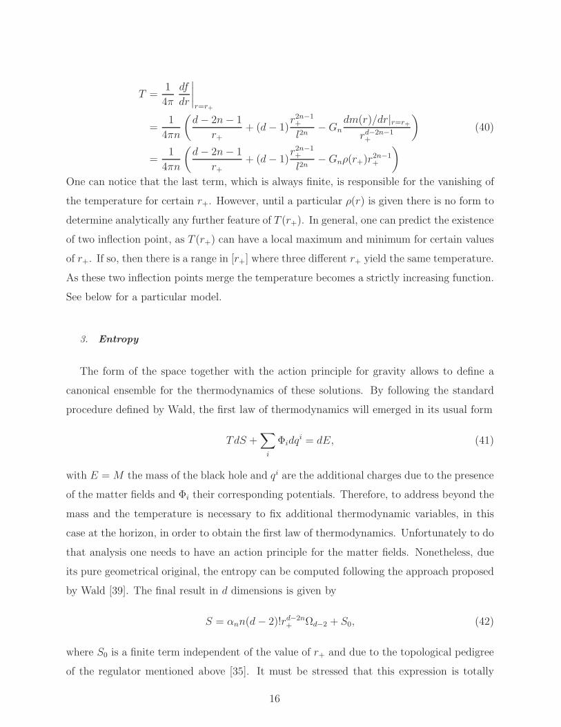
T =1

4π

df

dr

∣

∣

∣

∣

r=r+

=1

4πn

(

d− 2n− 1

r++ (d− 1)

r2n−1+

l2n−Gn

dm(r)/dr|r=r+

rd−2n−1+

)

(40)

=1

4πn

(

d− 2n− 1

r++ (d− 1)

r2n−1+

l2n−Gnρ(r+)r

2n−1+

)

One can notice that the last term, which is always finite, is responsible for the vanishing of

the temperature for certain r+. However, until a particular ρ(r) is given there is no form to

determine analytically any further feature of T (r+). In general, one can predict the existence

of two inflection point, as T (r+) can have a local maximum and minimum for certain values

of r+. If so, then there is a range in [r+] where three different r+ yield the same temperature.

As these two inflection points merge the temperature becomes a strictly increasing function.

See below for a particular model.

3. Entropy

The form of the space together with the action principle for gravity allows to define a

canonical ensemble for the thermodynamics of these solutions. By following the standard

procedure defined by Wald, the first law of thermodynamics will emerged in its usual form

TdS +∑

i

Φidqi = dE, (41)

with E = M the mass of the black hole and qi are the additional charges due to the presence

of the matter fields and Φi their corresponding potentials. Therefore, to address beyond the

mass and the temperature is necessary to fix additional thermodynamic variables, in this

case at the horizon, in order to obtain the first law of thermodynamics. Unfortunately to do

that analysis one needs to have an action principle for the matter fields. Nonetheless, due

its pure geometrical original, the entropy can be computed following the approach proposed

by Wald [39]. The final result in d dimensions is given by

S = αnn(d− 2)!rd−2n+ Ωd−2 + S0, (42)

where S0 is a finite term independent of the value of r+ and due to the topological pedigree

of the regulator mentioned above [35]. It must be stressed that this expression is totally

16

generic and functional independent of m(r). The value of r+ is not independent of the

function m(r), though. It can be noticed as well that this entropy does not follow an area

law by a power r2n−2+ but still defines an increasing function of r+. It is worth to stress that

for the particular case n = 1 the area law is well defined.

To pursue any further into an analytic analysis of the thermodynamics properties, for

instance the evaporation of these black holes, would require to define the temperature as an

function of the mass and additional chargess of the solution, which in turn needs at least

to consider a ρ(r) in particular. Unfortunately, this is not enough in general to obtain close

expressions. Because of that in the next sections will be considered a particular case which

will be analyzed through numerical methods.

B. Analysis of the Second Family of Solutions

1. Charges

As before, mass can be computed by computing the Noether charge associated with ∂t.

After regularization (one can follow [35]), is given

Q(∂t)∞ = M + E0 (43)

where E0 = 0 for even dimensions and corresponds to the vacuum energy for odd dimensions.

This is in complete analogy with [25, 31] but for the Chern Simons case. The difference with

results in [25, 31] arise due to the location of the horizons.

2. Temperature

In complete analogy with the previous case the temperature can be computed. For the

outer horizon this yields

T =1

4πn

(

d− 2n− 1

r++ (d− 1)

r+l2

−(

1 +r2+l2

)(

1

m(r)

dm(r)

dr

)

r=r+

)

(44)

=1

4πn

(

d− 2n− 1

r++ (d− 1)

r+l2

−(

1 +r2+l2

)1−n

r2n−1+ Gnρ(r+)

)

17

Notice that the last term is a correction to the expression obtained in [25] due to the finite

density of mass. This correction is responsible for the vanishing of the temperature for a

value of r+.

3. Entropy

In general the entropy can be computed as well in this case. This yields

S = αn(d− 2)!(r+

l

)d−2

Σγ

[

n

d− 2F

(

[1− n, 1− d/2], [2− d/2],−γl2 + r2+r2+

)]

+ S0, (45)

where Σγ is the area of the transverse section. It is matter of fact that equation (45) is same

expression obtained for the black hole solutions in [31] and the differences are due to the

value of r+ for a given value of M . S0 is due to topological term [35] added to regularize

the action principle [40].

For large r+ this entropy always approach an area law. It can be noticed as well that

for n = 1 the usual area law is recovered. This also occurs for γ = 0 for any value of n

or d. It is direct to check that for γ = 1 and γ = 0 these functions are monotonically

increasing functions of r+. Far more interesting is the fact that Sγ=−1(r+) can be negative

which imposes servere constrains in the space of parameters. As previously, r+ cannot be

determined analytically and so to proceed a numerical approach would be required. This

will be also considered for a next work.

VII. PLANCK ENERGY DENSITY

So far it has been shown that an anisotropic fluids is a suitable model to describe a

non-singular black hole. Still, we have not proposed any form for ρ(r) or m(r). Now we will

propose a d dimensional generalization of Hayward density [7]. For the 4D case and Einstein

Hilbert theory this model of density was used in references [1, 2] for describe Planck Stars.

Our generalization is given by:

ρ(r) =d− 1

Ωd−2

Qd−2M2

(Qd−2M + rd−1)2which yields m(r) =

Mrd−1

Qd−2M + rd−1. (46)

Here Q is introduced as regulator to avoid the presence of a singularity. It must be empha-

sized that Q has units of ℓd/(d−2)p , such that the energy density is of the order of a Planck

18

units near from origin and such that ρ(r) be able to satisfy the conditions in section II and

thus to describe a regular black hole density [1]. For instance, one can notice that

ρmax = ρ(0) =(d− 1)

Ωd−2Qd−2and m(r)|r≈0 ≈

rd−1

Qd−2, (47)

confirming that the energy density near of origin is of the order of Planck density.

A. Structure of Solutions

With the mass density in Eq.(46) is direct, by simple substitution, to obtain the form

of the solutions. Moreover, for r ≈ 0, both solutions behaves as de Sitter spaces with the

effective cosmological constant is given by Λ = (d− 1)(d− 2)l−2eff/2 > 0. l2eff differs for both

cases, however.

1. First family of solutions:

In the case f(r) is given by

f(r) = 1−((

M

Qd−2M + rd−1

)

− 1

l2n

)1

n

r2, (48)

which near r ≈ 0 behaves as

f(r)|r≈0 ≈ 1− r2

l2eff, (49)

a de Sitter space with1

l2eff=( 1

Qd−2− 1

l2n

)1

n

,

where it is required that l2n > Qd−2.

2. Second family of solutions:

In this case,

f(r) = 1−(

− 1

l2+

(

M

Qd−2M + rd−1

)1

n

)

r2, (50)

which also satisfies f(r)|r≈0 ≈ 1− (r/leff)2, in the case with

1

l2eff= − 1

l2+

1

Qd−2

n

, (51)

where again must be fulfilled that l2n > Qd−2.

19

0 1 2 3 4

-0,2

0,0

0,2

0,4

0,6

0,8

1,0

M>MCRI

MCRI

=4.25 M<M

CRI

f(r)

r

(a)f(r) for n = 1, d = 5.

0 2 4 60,0

0,5

M>MCRI

MCRI

=1.61 M<M

CRI

f(r)

r

(b)f(r) for n = 3, d = 8.

FIG. 1. f(r) for first family of solutions with toy values of Q = 1 and l = 8 .

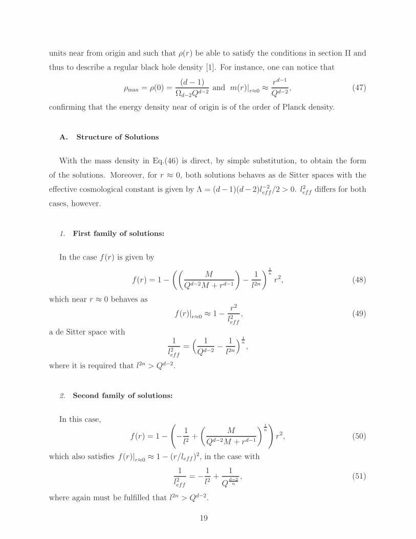
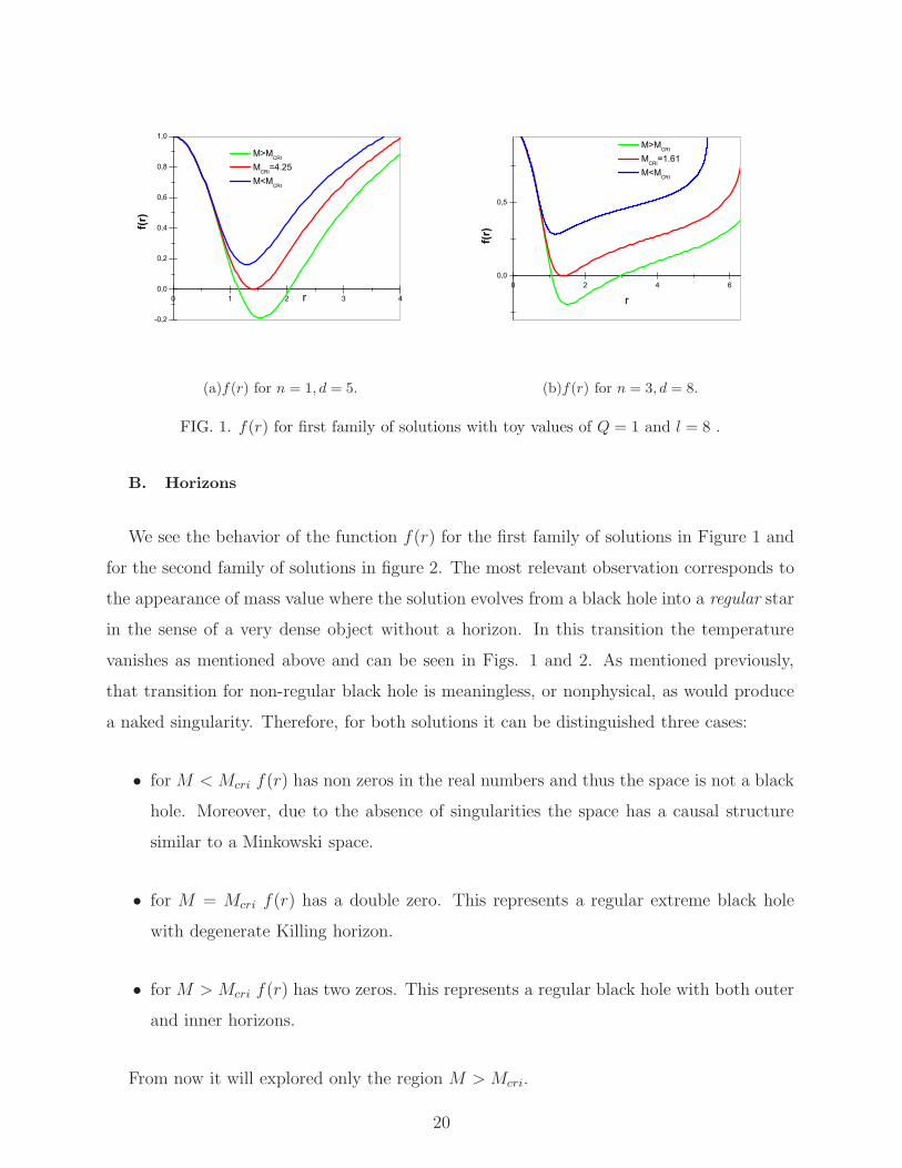
B. Horizons

We see the behavior of the function f(r) for the first family of solutions in Figure 1 and

for the second family of solutions in figure 2. The most relevant observation corresponds to

the appearance of mass value where the solution evolves from a black hole into a regular star

in the sense of a very dense object without a horizon. In this transition the temperature

vanishes as mentioned above and can be seen in Figs. 1 and 2. As mentioned previously,

that transition for non-regular black hole is meaningless, or nonphysical, as would produce

a naked singularity. Therefore, for both solutions it can be distinguished three cases:

• for M < Mcri f(r) has non zeros in the real numbers and thus the space is not a black

hole. Moreover, due to the absence of singularities the space has a causal structure

similar to a Minkowski space.

• for M = Mcri f(r) has a double zero. This represents a regular extreme black hole

with degenerate Killing horizon.

• for M > Mcri f(r) has two zeros. This represents a regular black hole with both outer

and inner horizons.

From now it will explored only the region M > Mcri.

20

0 1 2 3 4

-0,2

0,0

0,2

0,4

0,6

0,8

1,0

M>MCRI

MCRI

=2.8 M<M

CRI

f(r)

r

(a)f(r) for n = 2, d = 7.

0 2 4 6

-0,2

0,0

0,2

0,4

0,6

0,8

1,0

M>MCRI

MCRI

=1.8 M<M

CRI

f(r)

r

(b)f(r) for n = 3, d = 8.

FIG. 2. f(r) for second family of solutions with toy values of Q = 1 and l = 8 .

C. Temperature

Figures 3 and 4 display examples of the behavior of the temperatures, respectively. Figure

3(a) actually corresponds to both families of solutions since n = 1.

In general, one can notice that the temperature function has both a local maximum and

a local minimum, says at r+ = r∗ and r+ = r∗∗ respectively. AsdTdr+

vanishes in those points,

the heat capacity CQ = dMdr+

/(

dTdr+

)

diverges. See bellow. It must be noticed, however, that

for GR (n = 1) in four dimensions (d = 4) and for the second family of solutions with

n = 2 and d = 6 the temperature is always an increasing function of r+ and thus r∗ and r∗∗

disappear.

D. Heat Capacity

The heat capacity can be defined for Q constant as

CQ =dM

dr+

(

dT

dr+

)−1

. (52)

This definition, following the rules of thermodynamics, allows to determine that black

holes are locally stable/unstable under thermal fluctuation provided CQ > 0 or CQ < 0

respectively. With this in mind one can proceed with the analysis of the solutions. Figures

5 and 6 display examples of the behavior of the heat capacity. Notice that Figure 5(a)

represents both families of solutions as n = 1.

21

2 4 6 80,2

0,4

0,6

0,8

1,0Te

mpe

rature

d=4 d=5 d=6

r+

(a)T o for n = 1, d = 4, 5, 6.

2 4 60,00,10,20,30,40,50,60,70,80,91,01,11,21,31,41,5

d=8 d=9 d=10

Tempe

rature

r+

(b)T o for n = 3, d = 8, 9, 10.

FIG. 3. T o. Figure a) represents both families of solutions, and figure b) represents to the first

family of solutions, both with toy values of Q = 1 and l = 8.

2 4 60,0

0,2

0,4

0,6

0,8

1,0

1,2

1,4

Tempe

rature

r+

d=6 d=7 d=8

(a)T o for n = 2, d = 6, 7, 8.

2 4 60,0

0,2

0,4

0,6

0,8

1,0

1,2

1,4

1,6

Tempe

rature

r+

d=8 d=9 d=10

(b)T o for n = 3, d = 8, 9, 10.

FIG. 4. T o for second family of solutions with toy values of Q = 1 and l = 8 .

In general, it can be observed a phase transitions at both r∗ and r∗∗. Going from CQ > 0

for r+ > r∗∗ to CQ < 0 for r∗ < r+ < r∗∗. Finally CQ > 0 for r+ < r∗. Moreover, one can

notice as well that CQ vanishes as T → 0.

It is worth to mention that for GR (n = 1) in four dimensions (d = 4) and for the second

family of solutions with n = 2 and d = 6 there is no phase transitions. Moreover, although

cannot be observed at the figures, the specific heat in this case is a positive function of r+

which vanishes as T → 0 as well.

22

2 4 6 8-4000

-2000

0

2000

4000

6000

8000

10000

12000

14000

16000

d=4 d=5 d=6

Hea

t Cap

acity

r+

(a)CQ for n = 1, d = 4, 5, 6.

2 4 6 8-400-300-200-100

0100200300400500600700800900

100011001200

Hea

t Cap

acity

d=8 d=9 d=10

r+

(b)CQ for n = 3, d = 8, 9, 10.

FIG. 5. CQ. Figure a) represents both families of solutions, and figure b) represents to the first

family of solutions, both with toy values of Q = 1 and l = 8 .

2 4 6-2000

0

2000

4000

6000

8000

10000

12000

14000

Hea

t Cap

acity

r+

d=6 d=7 d=8

(a)CQ for n = 2, d = 6, 7, 8.

2 4 6

-2000

0

2000

4000

6000

8000

10000

12000

14000

Hea

t Cap

acity

r+

d=8 d=9 d=10

(b)CQ for n = 3, d = 8, 9, 10.

FIG. 6. CQ for second family of solutions with toy values of Q = 1 and l = 8 .

VIII. CONCLUSIONS AND DISCUSSIONS

In this work two families of regular black hole solutions have been discussed. Although

each family is a solution of a different Lovelock gravity in d dimensions both share to have

a single ground state, which is approached asymptotically by the solutions and is defined

by a single cosmological constant. These theories correspond to the Pure Lovelock theory

[26, 28, 30] and to the theory discussed in [25] which have a n-fold degenerated ground state.

First it must be noticed that solutions have a minimum value of the parameter M , called

23

Mcri above, to represent a black hole geometry. As expected, these solutions asymptotically,

says for large r, are indistinguishable from the previously known solutions [25, 28] in vacuum.

On the other hand, both families of solutions near the origin, for r ∼ 0, behaves as maximally

symmetric spaces which can be fixed, unambiguously, to be of positive curvature, i.e. the

parameters can be fixed such as the solutions approach de Sitter spaces, as required to model

a regular black hole, at their origins.

Concerning the thermodynamics of the solutions it was shown that, although both fam-

ilies of solutions differ, in general terms their thermodynamics presents the same features.

The associate temperatures of the horizons have, in general, a local maximum and a local

minimum at r∗ and r∗∗ respectively. Indeed, one can notice that there can be three different

values of r+ defining the same temperature. Because of this last, the heat capacity changes

from positive for r+ < r∗ to negative at r∗ < r+ < r∗∗ and finally to positive for r∗∗ < r+,

signing out two phase transitions of the system, from thermodynamically stable (CQ > 0)

into unstable (CQ < 0) and viceversa. Therefore, in general, there is a range of the black

hole radii, r∗ < r+ < r∗∗, or equivalently of the masses, where the black holes become ther-

modynamically unstable. The existence of a phase transition for the vacuum solutions in

[25] was known, and thus the phase transition at r∗∗ could have been anticipated. However

the existence of a second phase transition at r+ = r∗, and thus the existence a second stable

range for r+ < r∗, is a new feature proper of these regular black holes.

In order to analyze the thermodynamics in detail it was considered as model the gener-

alized Hayward energy density [7] defined in Eq,(46). Now, as mentioned in section II, the

conditions to be satisfied by the mass density are quite general, and thus it can be quite

interesting to explore other options in order to determine to what extent the arise of phase

transitions is a model dependent feature. For instance, it would be quite interesting to study

a generalization of the proposal in [5, 6]

ACKNOWLEDGMENTS

This work was partially funded by grants FONDECYT 1151107. R.A. likes to thank

DPI20140115 for some financial support.

24

Appendix A: Units

The unit system used throughout the text is slightly different from the ones presented in

other articles. Because of that the unit system will be reviewed here in some detail.

To begin with it has been fixed ~ = 1 and c = 1, the light speed. Therefore, the

mass/energy units is actually L−1, where L is some distant unit. Moreover, it must be

noticed that since ~ = 1 the action principle must be dimensionless.

As the αn coefficients must be fixed such that αnLn, with Ln the n term in the Lovelock

Lagrangian, be dimensionless, and [√gddx] = Ld then [αn] = L2n−d. By the same token, one

must notice that the mass density must satisfy [ρ(r)] = L−d. Finally, by direct observation,

the regulator in the generalized Hayward density must satisfy that [Q] = Ld/(d−2). One

can check that the term, α−1n r1+2n−dm(r), presented in the f(r) function for both solution,

satisfies[

α−1n

m(r)

rd−2n−1

]

= L0,

as expected for consistency.

[1] Tommaso De Lorenzo , Costantino Pacilio , Carlo Rovelli , Simone Speziale, “On the effective

metric of a planck star,” Gen.Rel.Grav. 47, 41 (2015), arXiv:1412.6015 [gr-qc] .

[2] Carlo Rovelli , Francesca Vidotto, “Planck stars,” Int.J.Mod.Phys. D 23, 1442026 (2014),

[arXiv:1401.6562v4 [gr-qc]] .

[3] James Bardeen, “Non-singular general-relativistic gravitacional collapse,” Proceedings of the

International Conference GR5, Tbilisi USSR (1968).

[4] Euro Spallucci , Anais Smailagic, “Regular black holes from semi-classical down to planckian

size,” Int. J. Mod. Phys. D 26, 1730013 (2017), arXiv:1701.04592v2 [hep-th] .

[5] Irina Dymnikova, “Vacuum nonsingular black hole,” Gen.Rel.Grav. 24, 235–242 (1992).

[6] Irina Dymnikova , Michal Korpusik, “Regular black hole remnants in de sitter space,”

Phys.Lett. B 686, 12–18 (2010).

[7] S. A. Hayward, “Formation and evaporation of regular black holes,” Phys.Rev.Lett. 96, 031103

(2006), [arXiv:gr-qc/0506126] .

25

[8] A. D. Sakharov, “Nachalnaia stadija rasshirenija vselennoj i vozniknovenije neodnorodnosti

raspredelenija veshchestva,” Sov. Phys. JETP 22, 241 (1966).

[9] C. Bambi and L. Modesto, “Rotating regular black holes,” Phys. Lett. B 721, 329–334 (2013),

[arXiv:gr-qc/0506126] .

[10] Sharmanthie Fernando, “Bardeen-de sitter black holes,” Int.J.Mod.Phys. D 26, 1750071

(2017), arXiv:1611.05337 [gr-qc].

[11] Dharm Veer Singh , Naveen K. Singh, “Anti-evaporation of bardeen de-sitter black holes,”

Annals Phys. 383, 600–609 (2017), arXiv:1704.01831 .

[12] Md Sabir Ali and Sushant G. Ghosh, “Thermodynamics of rotating bardeen black holes: Phase

transitions and thermodynamics volume,” Phys. Rev. D 99, 024015 (2019).

[13] Amna Khawer Abdul Jawad, “Thermodynamic consequences of well-known regular black holes

under modified first law,” Eur.Phys.J. C 78, 837 (2018).

[14] Manuel E. Rodrigues Marcos V. de S. Silva, “Regular black holes in f(g) gravity,” Eur. Phys.

J. C 78, 638 (2018), arXiv:1808.05861 [gr-qc].

[15] Athanasios G. Tzikas, “Bardeen black hole chemistry,” Physics Letters B 788, 219–224 (2019),

arXiv:1811.01104 [gr-qc].

[16] Stefano Liberati Costantino Pacilio Matt Visser Raul Carballo-Rubio, Francesco Di Filippo,

“On the viability of regular black holes,” JHEP 2018: 23 (2018), arXiv:1805.02675 [gr-qc].

[17] Cosimo Bambi Qiqi Zhang, Leonardo Modesto, “A general study of regular and singu-

lar black hole solutions in einstein’s conformal gravity,” Eur. Phys. J. C 78, 506 (2018),

arXiv:1805.00640 [gr-qc]].

[18] Md Sabir Ali and Sushant G. Ghosh, “Exact d-dimensional bardeen-de sitter black holes and

thermodynamics,” Phys. Rev. D 98, 084025 (2018).

[19] Arun Kumar, Dharm Veer Singh, Sushant G. Ghosh, “D-dimensional bardeen-ads black holes

in einstein-gauss-bonnet theory,” (2018), arXiv:1808.06498 [gr-qc] .

[20] Sushant G. Ghosh , Dharm Veer Singh, and Sunil D. Mahara, “Regular black holes in einstein-

gauss-bonnet gravity,” Phys. Rev. D 97, 104050 (2018).

[21] Lovelock D., “The einstein tensor and its generalizations,” J.Math.Phys. 12, 498–501 (1971).

[22] M. Banados , C. Teitelboim and J. Zanelli, “Dimensionally continued black holes,” Phys. Rev.

D 49, 975–986 (1994), [arXiv:gr-qc/9307033] .

[23] T. Eguchi , P. B. Gilkey and A. J. Hanson, “Gravitation, gauge theories and differential

26

geometry,” Phys. Rept. 66, 213 (1980).

[24] Megha Padi Wei Song Andrew Strominger Dionysios Anninos, Wei Li, “Warped ads3 black

holes,” JHEP 0903, 130 (2009), arXiv:0807.3040 [hep-th].

[25] J. Crisostomo , R. Troncoso and J. Zanelli, “Black hole scan,” Phys. Rev. D 62, 084013 (2000),

arXiv:hep-th/0003271 .

[26] Naresh Dadhich, “On lovelock vacuum solution,” Math.Today 26, 37 (2011),

[arXiv:1006.0337 [hep-th]] .

[27] Naresh Dadhich , Josep M. Pons , Kartik Prabhu, “Thermodynamical universality of the

lovelock black holes,” Gen. Rel. Grav. 44, 2595–2601 (2012), arXiv:1110.0673 [gr-qc]] .

[28] R. G. Cai and N. Ohta, “Black holes in pure lovelock gravities,” Phys. Rev. D 74, 064001

(2006), arXiv:hep-th/0604088 .

[29] R. G. Cai , L. M. Cao and N. Ohta, “Black holes without mass and entropy in lovelock

gravity,” Phys. Rev. D 81, 024018 (2010), arXiv:0911.0245 [hep-th] .

[30] Naresh Dadhich , Sudan Hansraj , Sunil D. Maharaj, “Universality of isothermal fluid spheres

in lovelock gravity,” Phys. Rev. D 93, 044072 (2016), [arXiv:1510.07490 [gr-qc]].

[31] R. Aros, R. Troncoso and J. Zanelli, “Black holes with topologically nontrivial ads asymp-

totics,” Phys. Rev. D 63, 084015 (2001), arXiv:hep-th/0011097 .

[32] R. Aros, “de sitter thermodynamics: A glimpse into non equilibriumy,” Phys. Rev. D 77,

104013 (2008), arXiv:0801.4591 [gr-qc] .

[33] J. Lee and Robert M. Wald, “Local symmetries and constraints,”

J. Math. Phys. 31, 725–743 (1990).

[34] Kostas Skenderis, “Lecture notes on holographic renormalization,” Class. Quant. Grav. 19,

5849–5876 (2002), hep-th/0209067.

[35] Georgios Kofinas and Rodrigo Olea, “Universal Kounterterms in Lovelock AdS gravity,”

Fortsch.Phys. 56, 957–963 (2008), arXiv:0806.1197 [hep-th].

[36] Rodrigo Olea, “Regularization of odd-dimensional AdS gravity: Kounterterms,” JHEP 04,

073 (2007), arXiv:hep-th/0610230.

[37] Georgios Kofinas and Rodrigo Olea, “Universal regularization prescription for Lovelock AdS

gravity,” JHEP 11, 069 (2007), arXiv:0708.0782 [hep-th].

[38] P. Mora , R. Olea , R. Troncoso and J. Zanell, “Vacuum energy in odd-dimensional ads

gravity,” (2004), arXiv:hep-th/0412046 .

27

[39] R. M. Wald, “Black hole entropy is noether charge,” Phys. Rev. D 48, R3427–R3431 (1993),

arXiv:gr-qc/9307038 .

[40] R. Aros, “Boundary conditions in first order gravity: Hamiltonian and ensemble,” Phys. Rev.

D 73, 024004 (2006), arXiv:gr-qc/0507091 .

28