Density functional theory (DFT) and the concepts of the ...susi.theochem.tuwien.ac.at › ... ›...
80
Density functional theory (DFT) and the concepts of the augmented-plane-wave plus local orbital (L)APW+lo method Karlheinz Schwarz Institute for Material Chemistry TU Wien Vienna University of Technology
Transcript of Density functional theory (DFT) and the concepts of the ...susi.theochem.tuwien.ac.at › ... ›...
Density functional theory (DFT) and the concepts of the augmented-plane-wave plus local orbital (L)APW+lo method
Karlheinz SchwarzInstitute for Material Chemistry
TU WienVienna University of Technology

K.Schwarz, P.Blaha, S.B.Trickey,Molecular physics, 108, 3147 (2010)
DFTAPW LAPWJ.C.Slater O.K.Andersen
Wien2k is used worldwideby about 2500 groups
Electronic structure of solids and surfaces
hexagonal boron nitride on Rh(111)2x2 supercell (1108 atoms per cell)
Phys.Rev.Lett. 98, 106802 (2007)
The WIEN2k code: comments
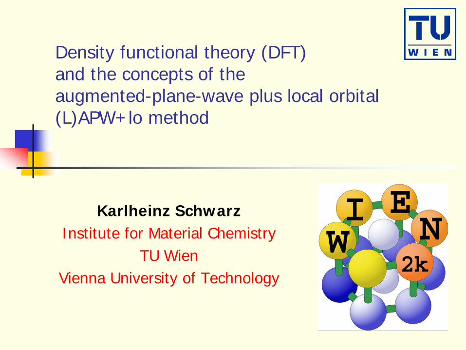
Walter Kohn: density functional theory (DFT), 1965 J.C.Slater: augmented plane wave (APW) method, 1937O.K.Andersen: Linearized APW (LAPW), 1975Wien2k code: developed during the last 35 years
In the year 2000 (2k) the WIEN code (from Vienna) was called wien2k One of the most accurate DFT codes for solids All electron, relativistic, full- potential method Widely used in academia and industry
Applications: solids: insulators , covalently bonded systems, metals Surfaces: catalysis Electronic, magnetic, elastic , optical ,…properties Many application in literature See www.wien2k.at

Review articles
K.Schwarz, P.Blaha, S.B.Trickey, Electronic structure of solids with WIEN2kMolecular physics, 108, 3147 (2010)
K.Schwarz, Computation of Materials Properties at the Atomic Scale InTech, (2015) Chapter 10, 275-310, open access bookISBN 978-953-51-2126-8 (2015) dx.doi.org/10.5772/59108
K.Schwarz, P.Blaha, G.K.H.Madsen, Electronic structure calculations of solids using the WIEN2k package for material SciencesComp.Phys.Commun.147, 71-76 (2002)
K.Schwarz, DFT calculations of solids with LAPW and WIEN2kSolid State Chem.176, 319-328 (2003)
K.Schwarz, P.Blaha, Electronic structure of solids and surfaces with WIEN2kin Practical Aspects of Computational Chemistry I: An Overview of the Last Two Decades and Current Trends,
J.Leszczyncski, M.K.Shukla (Eds),
Springer Science+Business Media B.V. (2012) Chapter 7, 191-207, ISBN 978-94-007-0918-8
S.Cottenier,Density Functionl Theory and the famliy of (L)APW methods : A step by step introduction 2002-2012 /(2nd edition); ISBN 978-90-807215-1-7 Freely available at: http://www.wien2k.at/reg-user/textbooks I
Aspects at this workshop
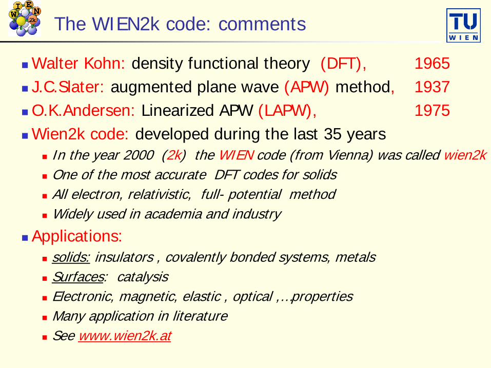
Atomic structure Periodic boundary condition (approximation)
Quantum mechanical treatment DFT (functionals) and beyond (GW, DMFT, RPA, BSE, …)
How to solve the QM (basis set) LAPW method and local orbitals as implemented in WIEN2k
Applications Verwey transition, EFG, NMR, surfaces, spectra ….
Software development Accuracy, efficiency, system size, user-friendliness, commercial
Insight and understanding Analysis to find trends, computer experiments (artificial cases)
Combination of expertise Chemistry, physics, mathematics, computer science, application
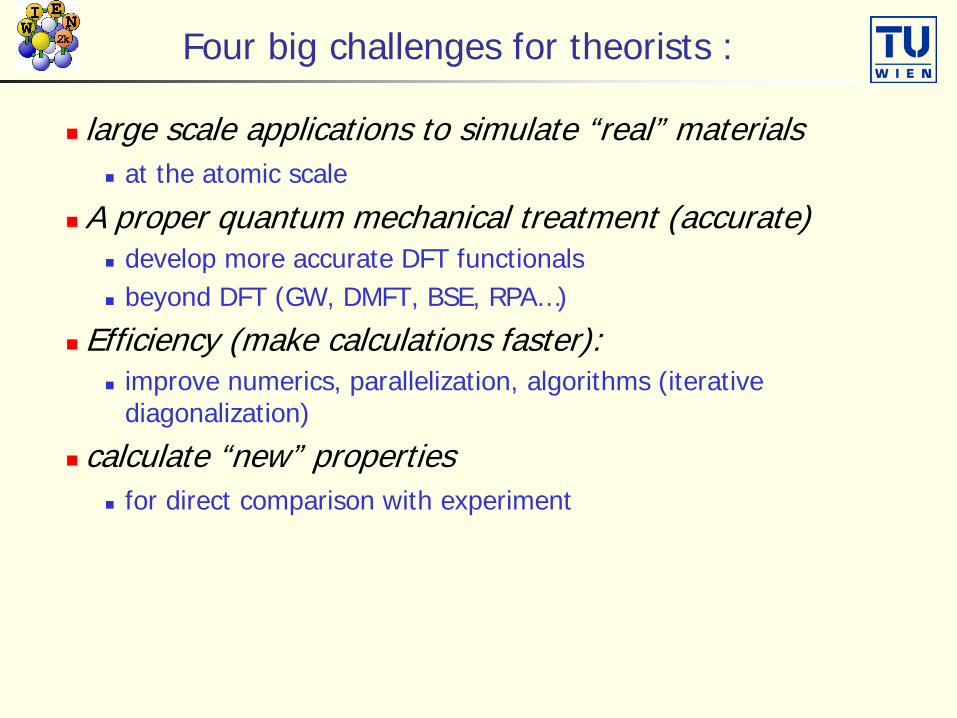
Four big challenges for theorists :
large scale applications to simulate “real” materials at the atomic scale
A proper quantum mechanical treatment (accurate) develop more accurate DFT functionals beyond DFT (GW, DMFT, BSE, RPA…)
Efficiency (make calculations faster): improve numerics, parallelization, algorithms (iterative
diagonalization)
calculate “new” properties for direct comparison with experiment

The atomic structure
A crystal is represented by a unit cell We assume periodic boundary condition (approximation) The unit cell is repeated to infinity (makes calculations feasible) A real crystal is finite (with surfaces, impurities, defects …) Nano materials differ from bulk Symmetry helps (space group, Bloch theorem, …)
In theory The atomic structure is an input and thus well defined. Artificial structures can be studied too
In experiment The atomic structure is not perfectly known Single crystals, micro crystals, powder samples, nano e.g. by X-ray: averaged with uncertainties (defects, disorder)

A few solid state concepts
Crystal structure Unit cell (defined by 3 lattice vectors) leading to 7 crystal systems Bravais lattice (14) Atomic basis (Wyckoff position) Symmetries (rotations, inversion, mirror planes, glide plane, screw axis) Space group (230) Wigner-Seitz cell Reciprocal lattice (Brillouin zone)
Electronic structure Periodic boundary conditions Bloch theorem (k-vector), Bloch function Schrödinger equation (HF, DFT)

b
c
αβ
γa
Unit cell: a volume in space that fills space entirely when translated by all lattice vectors.
The obvious choice:
a parallelepiped defined by a, b, c, three basis vectors with
the best a, b, c are as orthogonal as possible
the cell is as symmetric as possible (14 types)
A unit cell containing one lattice point is called primitive cell.
Unit cell
Assuming an ideal infinite crystal we define a unit cell by

Axis system
primitive
a = b = cα = β = γ = 90°
body centered face centered
P (cP) I (bcc) F (fcc)
Crystal system: e.g. cubic
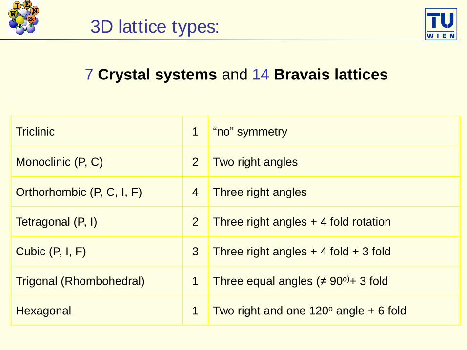
3D lattice types:
Triclinic 1 “no” symmetry
Monoclinic (P, C) 2 Two right angles
Orthorhombic (P, C, I, F) 4 Three right angles
Tetragonal (P, I) 2 Three right angles + 4 fold rotation
Cubic (P, I, F) 3 Three right angles + 4 fold + 3 fold
Trigonal (Rhombohedral) 1 Three equal angles (≠ 90o)+ 3 fold
Hexagonal 1 Two right and one 120o angle + 6 fold
7 Crystal systems and 14 Bravais lattices
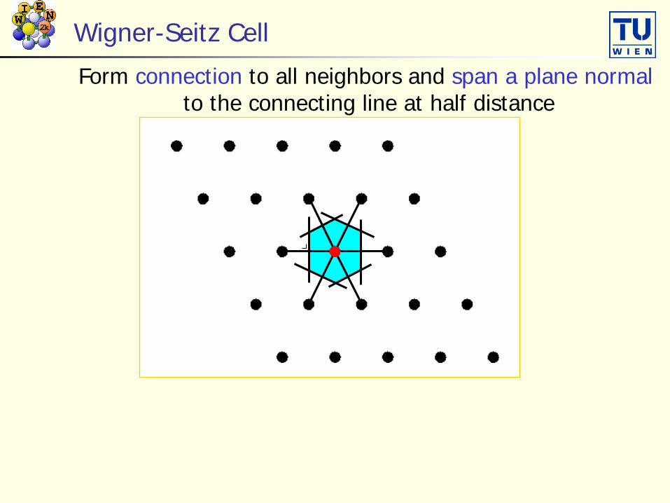
Wigner-Seitz Cell
Form connection to all neighbors and span a plane normalto the connecting line at half distance

The quantum mechanical treatment
The electronic structure requires a QM treatment The main scheme is density functional theory (DFT)
It is a mean field approach and requires approximations According to Hohenberg Kohn it is sufficient to know the electron
density of a system to determine its total energy. The many electron wave function (which depends on many variables) is not needed. In principle this is an enormous simplification, but in practice approximations must be made.
The direction of improving the QM treatment is summarized pictorially in Jabob’s ladder:
There are schemes which go beyond DFT: GW method (for excitations or band gaps) The Bethe Salpeter equation (BSE) for excitons (core hole - electron) Dynamical mean field theory (DMFT) based on DFT (wien2wannier)

Bloch-Theorem:
[ ] )()()(21 2 rErrV Ψ=Ψ+∇−
1-dimensioanl case:
V(x) has lattice periodicity (“translational invariance”): V(x)=V(x+a)
The electron density ρ(x) has also lattice periodicity, however, the wave function does NOT:
1)()(:)()()()(
*
*
=⇒Ψ=+Ψ
ΨΨ=+=
µµµ
ρρ
xaxbutxxaxx
Application of the translation τ g-times:
)()()( xgaxx gg Ψ=+Ψ=Ψ µτ
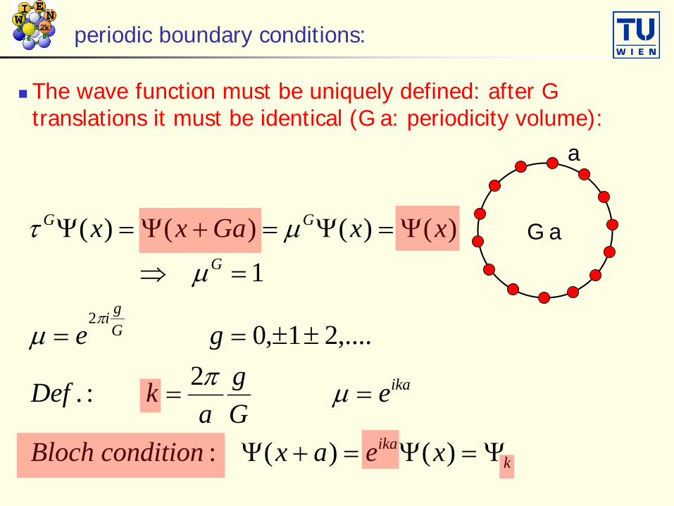
periodic boundary conditions:
The wave function must be uniquely defined: after G translations it must be identical (G a: periodicity volume):
kika
ika
Ggi
G
GG
xeaxconditionBloch
eGg
akDef
ge
xxGaxx
Ψ=Ψ=+Ψ
==
±±==
=⇒
Ψ=Ψ=+Ψ=Ψ
)()(:
2:.
,....21,0
1)()()()(
2
µπµ
µ
µτ
π
a
G a

Bloch functions:
Wave functions with Bloch form:
)()(:)()( axuxuwherexuex ikxk +==Ψ
Phase factor lattice periodic functionRe [ψ(x)]
x
Replacing k by k+K, where K is a reciprocal lattice vector,fulfills again the Bloch-condition. k can be restricted to the first Brillouin zone .
ak
ae
Ka
i πππ
<<−= 12

Concepts when solving Schrödingers-equation in solids
non relativisticsemi-relativisticfully-relativistic
(non-)selfconsistent“Muffin-tin” MTatomic sphere approximation (ASA)Full potential : FPpseudopotential (PP)
Hartree-Fock (+correlations)Density functional theory (DFT)
Local density approximation (LDA)Generalized gradient approximation (GGA)Beyond LDA: e.g. LDA+U
Non-spinpolarizedSpin polarized(with certain magnetic order)
non periodic (cluster)periodic (unit cell)
plane waves : PWaugmented plane waves : APWatomic oribtals. e.g. Slater (STO), Gaussians (GTO),
LMTO, numerical basis
Basis functions
Treatment of spin
Representationof solid
Form ofpotential
exchange and correlation potentialRelativistic treatment
of the electrons
Schrödinger – equation(Kohn-Sham equation)
ki
ki
kirV ϕεϕ =
+∇− )(
21 2

DFT vs. MBT (many body theory)

Coulomb potential: nuclei all electrons including
self-interaction
Quantum mechanics: exchange correlation (partly) cancel
self-interaction
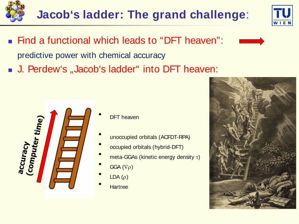
Jacob‘s ladder: The grand challenge:
Find a functional which leads to “DFT heaven”: predictive power with chemical accuracy
J. Perdew‘s „Jacob‘s ladder“ into DFT heaven:
• DFT heaven
• unoccupied orbitals (ACFDT-RPA)• occupied orbitals (hybrid-DFT)• meta-GGAs (kinetic energy density τ)• GGA (∇ρ)• LDA (ρ)• Hartree

Hohenberg-Kohn theorem: (exact)
The total energy of an interacting inhomogeneous electron gas in the presence of an external potential Vext(r ) is a functional of the density ρ
][)()( ρρ FrdrrVE ext += ∫
In KS the many body problem of interacting electrons and nuclei is mapped to a one-electron reference system that leads to the same density as the real system.
][||)()(
21)(][ ρρρρρ xcexto Erdrd
rrrrrdrVTE +′
−′′
++= ∫∫
Ekineticnon interacting
Ene Ecoulomb Eee Exc exchange-correlation
Kohn-Sham: (still exact!)
DFT Density Functional Theory
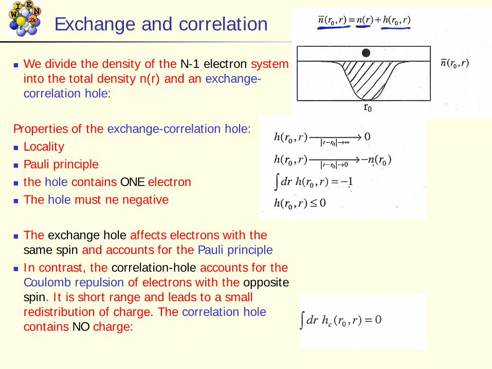
Exchange and correlation
We divide the density of the N-1 electron system into the total density n(r) and an exchange-correlation hole:
Properties of the exchange-correlation hole: Locality Pauli principle the hole contains ONE electron The hole must ne negative
The exchange hole affects electrons with the same spin and accounts for the Pauli principle
In contrast, the correlation-hole accounts for the Coulomb repulsion of electrons with the opposite spin. It is short range and leads to a small redistribution of charge. The correlation holecontains NO charge:
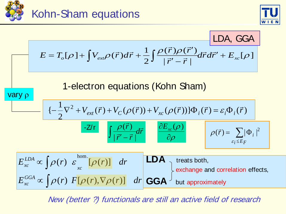
Kohn-Sham equations
rdrr
r
∫ −′ ||)(ρ
ρρ
∂∂ )(xcE
][||)()(
21)(][ ρρρρρ xcexto Erdrd
rrrrrdrVTE +′
−′′
++= ∫∫
1-electron equations (Kohn Sham)
)()())}(())(()(21{ 2 rrrVrVrV iiixcCext
Φ=Φ+++∇− ερρ
∑≤
Φ=FEi
irε
ρ 2||)(
LDA, GGA
vary ρ
LDA treats both, exchange and correlation effects,
GGA but approximately
-Z/r
drrrFrE
drrrEGGAxc
xc
LDAxc
)](),([)(
)]([)(.hom
ρρρ
ρερ
∇∝
∝
∫∫
New (better ?) functionals are still an active field of research
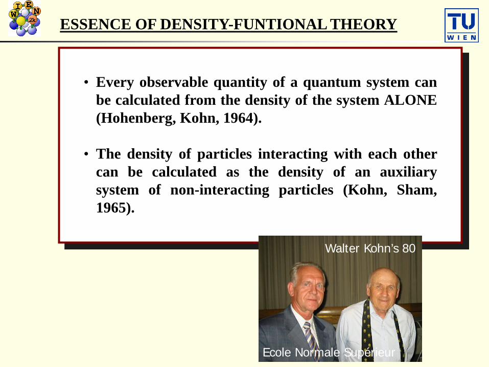
ESSENCE OF DENSITY-FUNTIONAL THEORY
• Every observable quantity of a quantum system canbe calculated from the density of the system ALONE(Hohenberg, Kohn, 1964).
• The density of particles interacting with each othercan be calculated as the density of an auxiliarysystem of non-interacting particles (Kohn, Sham,1965).
Walter Kohn’s 80
Ecole Normale Supérieur

Walter Kohn, Nobel Prize 1998 Chemistry
“Self-consistent Equations including Exchange and Correlation Effects”W. Kohn and L. J. Sham, Phys. Rev. 140, A1133 (1965)
Literal quote from Kohn and Sham’s paper:“… We do not expect an accurate description of chemical binding.”
50 years ago

DFT ground state of iron
LSDA NM fcc in contrast to
experiment
GGA FM bcc Correct lattice
constant
Experiment FM bcc
GGAGGA
LSDA
LSDA

DFT thanks to Claudia Ambrosch (previously in Graz)
GGA follows LDA
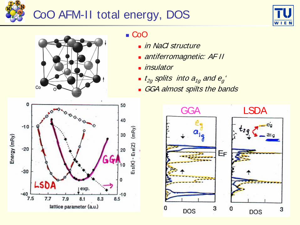
CoO AFM-II total energy, DOS
CoO in NaCl structure antiferromagnetic: AF II insulator t2g splits into a1g and eg‘ GGA almost spilts the bands
GGA LSDA

CoO why is GGA better than LSDA
Central Co atom distinguishes
between
and
Angular correlation
LSDAxc
GGAxcxc VVV ↑↑↑ −=∆ ↑Co
↓Co↑Co
↑Co↓Co
O
Co↑

FeF2: GGA works surprisingly well
FeF2: GGA splitst2g into a1g and eg’
Fe-EFG in FeF2:LSDA: 6.2GGA: 16.8exp: 16.5
LSDA
GGA
agree
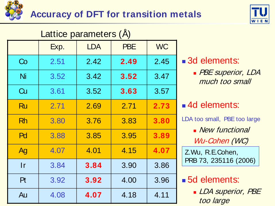
Accuracy of DFT for transition metals
3d elements: PBE superior, LDA
much too small
4d elements:LDA too small, PBE too large
New functionalWu-Cohen (WC)
5d elements: LDA superior, PBE
too large
Exp. LDA PBE WC
Co 2.51 2.42 2.49 2.45
Ni 3.52 3.42 3.52 3.47
Cu 3.61 3.52 3.63 3.57
Ru 2.71 2.69 2.71 2.73
Rh 3.80 3.76 3.83 3.80
Pd 3.88 3.85 3.95 3.89
Ag 4.07 4.01 4.15 4.07
Ir 3.84 3.84 3.90 3.86
Pt 3.92 3.92 4.00 3.96
Au 4.08 4.07 4.18 4.11
Lattice parameters (Å)
Z.Wu, R.E.Cohen, PRB 73, 235116 (2006)
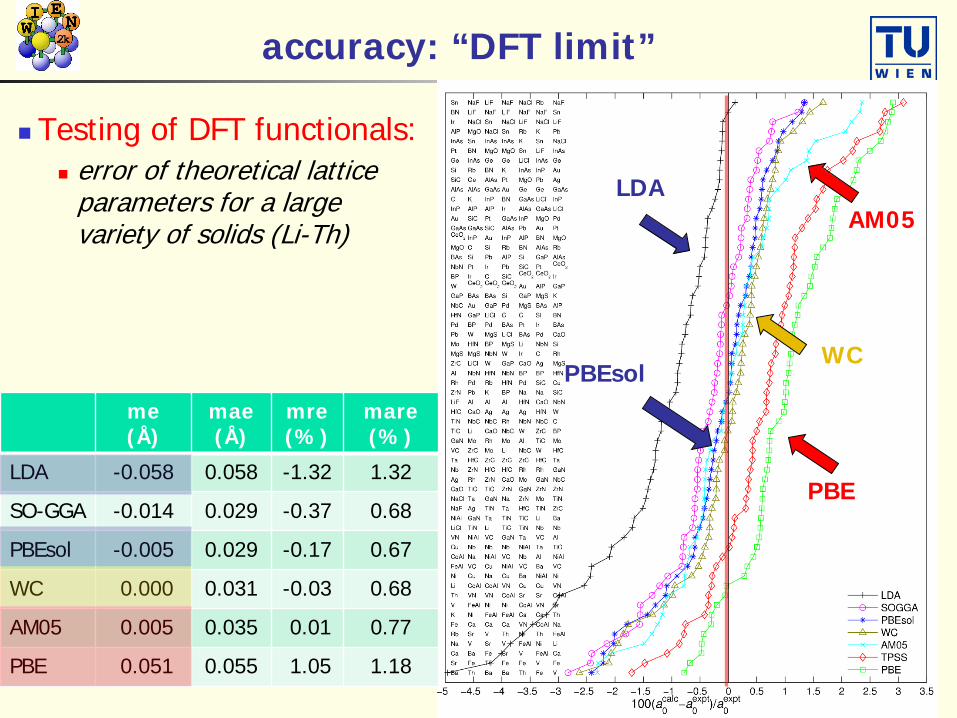
accuracy: “DFT limit”
Testing of DFT functionals: error of theoretical lattice
parameters for a large variety of solids (Li-Th)
me(Å)
mae(Å)
mre(%)
mare(%)
LDA -0.058 0.058 -1.32 1.32
SO-GGA -0.014 0.029 -0.37 0.68
PBEsol -0.005 0.029 -0.17 0.67
WC 0.000 0.031 -0.03 0.68
AM05 0.005 0.035 0.01 0.77
PBE 0.051 0.055 1.05 1.18
LDA
PBE
PBEsol
AM05
WC

Can LDA be improved ?
better GGAs and meta-GGAs (ρ, ∇ρ, τ): usually improvement, but often too small.
LDA+U: for correlated 3d/4f electrons, treat strong Coulomb repulsion via Hubbard U parameter (cheap, “empirical U” ?)
Exact exchange: imbalance between exact X and approximate C hybrid-DFT (mixing of HF + GGA; “mixing factor” ?) exact exchange + RPA correlation (extremely expensive)
GW: gaps in semiconductors, expensive!
Quantum Monte-Carlo: very expensive
DMFT: for strongly correlated (metallic) d (f) -systems (expensive)
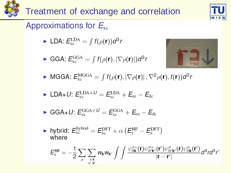
Treatment of exchange and correlation
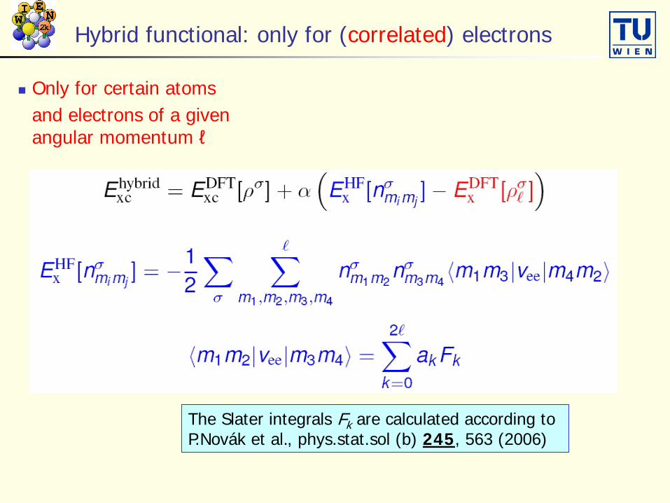
Hybrid functional: only for (correlated) electrons
Only for certain atomsand electrons of a given angular momentum ℓ
The Slater integrals Fk are calculated according to P.Novák et al., phys.stat.sol (b) 245, 563 (2006)

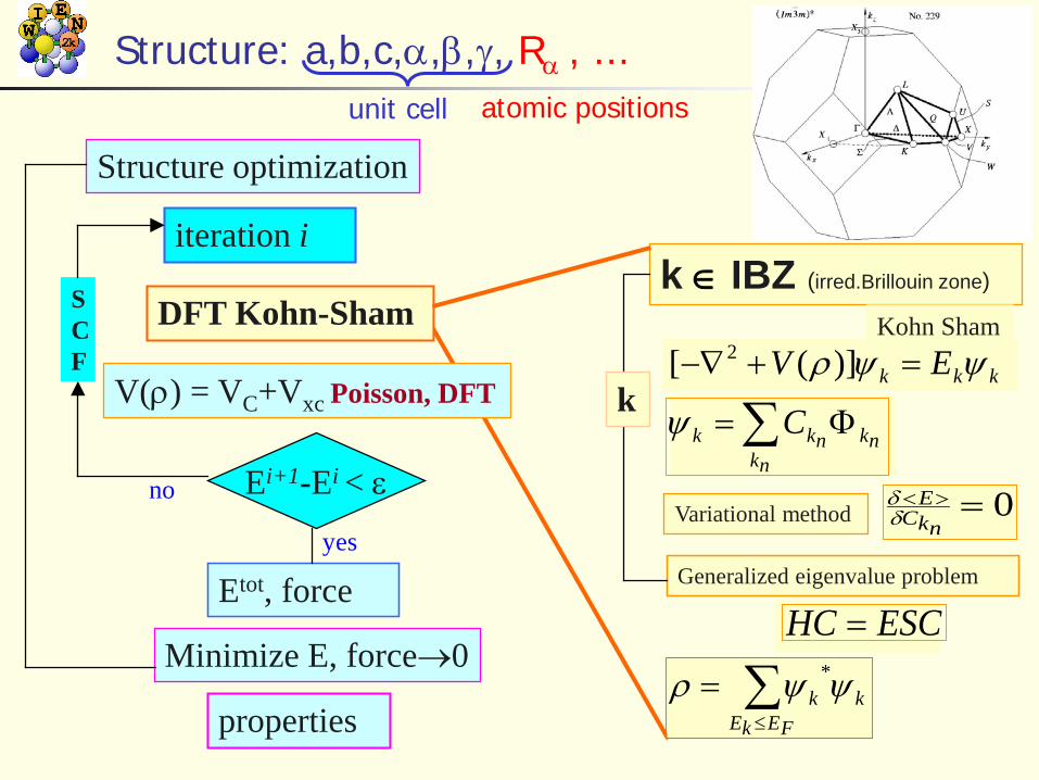
Structure: a,b,c,α,β,γ, Rα , ...
Ei+1-Ei < ε
Etot, force
Minimize E, force→0
properties
yes
V(ρ) = VC+Vxc Poisson, DFT
DFT Kohn-Sham
Structure optimization
iteration i
no
SCF
k ∈ IBZ (irred.Brillouin zone)
kkk EV ψψρ =+−∇ )]([ 2Kohn Sham
∑ Φ=nk
nknkk Cψ
Variational method 0=><nkC
Eδδ
Generalized eigenvalue problem
ESCHC =
∑≤
=FEkE
kk ψψρ *
k
unit cell atomic positionsk-mesh in reciprocal space
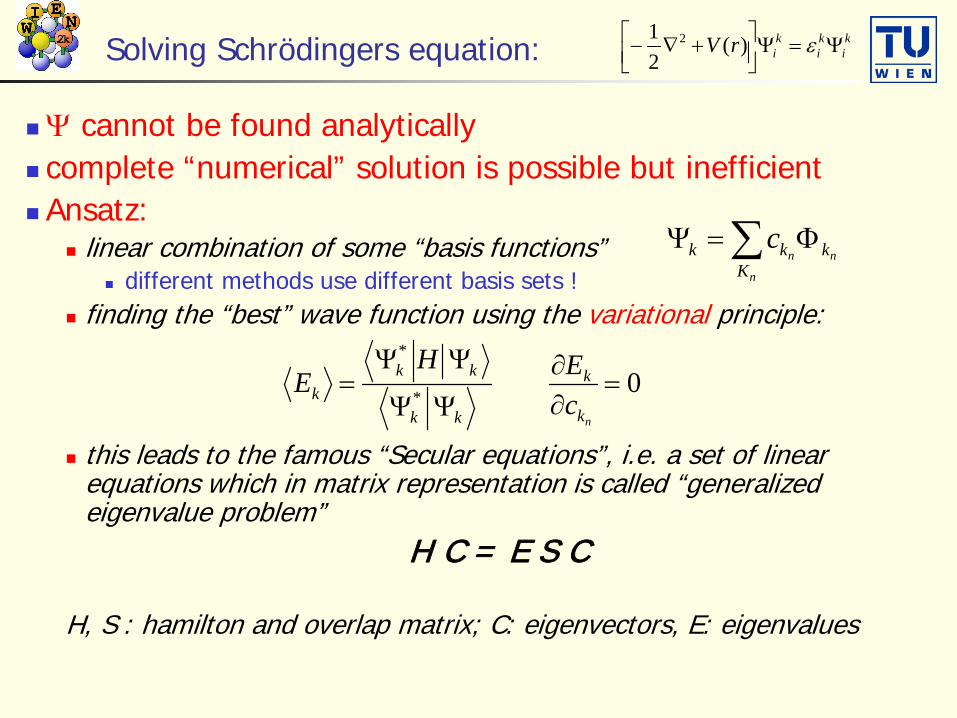
Solving Schrödingers equation:
Ψ cannot be found analytically complete “numerical” solution is possible but inefficient Ansatz:
linear combination of some “basis functions” different methods use different basis sets !
finding the “best” wave function using the variational principle:
this leads to the famous “Secular equations”, i.e. a set of linear equations which in matrix representation is called “generalized eigenvalue problem”
H C = E S C
H, S : hamilton and overlap matrix; C: eigenvectors, E: eigenvalues
ki
ki
kirV Ψ=Ψ
+∇− ε)(
21 2
∑ Φ=Ψn
nnK
kkk c
0*
*
=∂∂
ΨΨ
ΨΨ=
nk
k
kk
kkk c
EHE

Basis Sets for Solids
plane waves pseudo potentials PAW (projector augmented wave) by P.E.Blöchl
space partitioning (augmentation) methods LMTO (linear muffin tin orbitals)
ASA approx., linearized numerical radial function + Hankel- and Bessel function expansions full-potential LMTO
ASW (augmented spherical wave) similar to LMTO
KKR (Korringa, Kohn, Rostocker method) solution of multiple scattering problem, Greens function formalism equivalent to APW
(L)APW (linearized augmented plane waves) LCAO methods
Gaussians, Slater, or numerical orbitals, often with PP option)
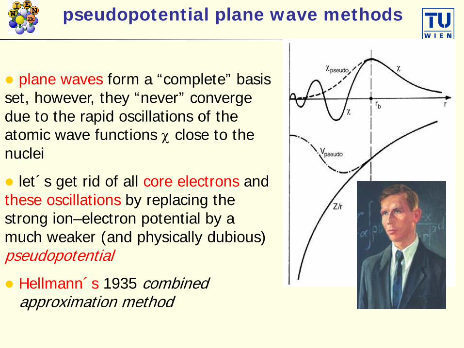
pseudopotential plane wave methods
plane waves form a “complete” basis set, however, they “never” converge due to the rapid oscillations of the atomic wave functions χ close to the nuclei
let´s get rid of all core electrons and these oscillations by replacing the strong ion–electron potential by a much weaker (and physically dubious) pseudopotential
Hellmann´s 1935 combined approximation method

ψ
ρVeff
Pseudo-ψ
Pseudo-ρ
Pseudo-potential
x
xx
r
“real” potentials vs. pseudopotentials
• “real” potentials contain the Coulomb singularity -Z/r• the wave function has a cusp and many wiggles, • chemical bonding depends mainly on the overlap of the
wave functions between neighboring atoms (in the region between the nuclei)
exact form of V only needed beyond rcore rcore
exact Ψ
exact V
exact ρ
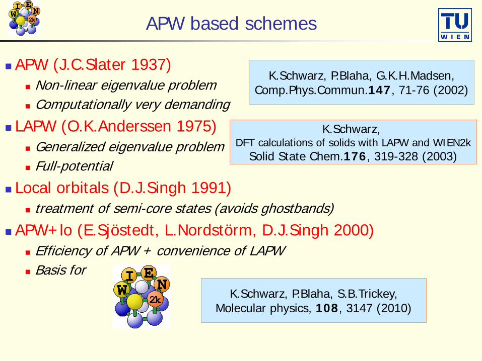
APW based schemes
APW (J.C.Slater 1937) Non-linear eigenvalue problem Computationally very demanding
LAPW (O.K.Anderssen 1975) Generalized eigenvalue problem Full-potential
Local orbitals (D.J.Singh 1991) treatment of semi-core states (avoids ghostbands)
APW+lo (E.Sjöstedt, L.Nordstörm, D.J.Singh 2000) Efficiency of APW + convenience of LAPW Basis for
K.Schwarz, P.Blaha, G.K.H.Madsen,Comp.Phys.Commun.147, 71-76 (2002)
K.Schwarz, DFT calculations of solids with LAPW and WIEN2k
Solid State Chem.176, 319-328 (2003)
K.Schwarz, P.Blaha, S.B.Trickey,Molecular physics, 108, 3147 (2010)

PW:
APW Augmented Plane Wave method
The unit cell is partitioned into:atomic spheresInterstitial region
rKkie
).( +
Atomic partial waves
∑ ′′m
mKm rYruA
)ˆ(),( ε
join
Rmt
unit cell
Basis set:
ul(r,ε) are the numerical solutions of the radial Schrödinger equationin a given spherical potentialfor a particular energy εAlm
K coefficients for matching the PW
Ir ∈
Plane Waves(PWs)
PWs atomic

Slater‘s APW (1937)
Atomic partial waves
Energy dependent basis functionslead to a
Non-linear eigenvalue problem
∑ ′′m
mKm rYrua
)ˆ(),( ε
Numerical search for those energies, for which the det|H-ES| vanishes. Computationally very demanding.
“Exact” solution for given MT potential!
H HamiltonianS overlap matrix

Linearization of energy dependence
LAPW suggested by
)ˆ()],()(),()([ rYrEukBrEukA mnm
mnmkn
∑ +=Φ
Atomic sphere
PW
O.K.Andersen,Phys.Rev. B 12, 3060 (1975)
expand ul at fixed energy El and add
Almk, Blm
k: join PWs in value and slope
General eigenvalue problem (diagonalization)
additional constraint requires more PWs than APW
LAPW
ε∂∂= /ll uu
APW
bonding
antibonding
center

shape approximations to “real” potentials
Atomic sphere approximation (ASA) overlapping spheres “fill” all volume potential spherically symmetric
“muffin-tin” approximation (MTA) non-overlapping spheres with spherically
symmetric potential + interstitial region with V=const.
“full”-potential no shape approximations to V
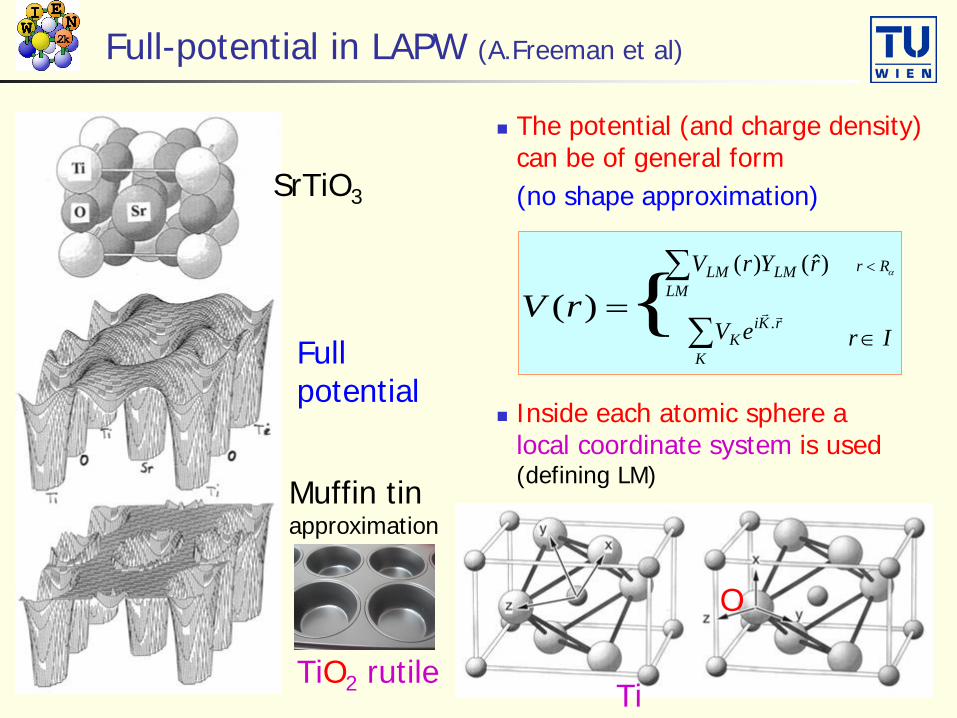
Full-potential in LAPW (A.Freeman et al)
The potential (and charge density) can be of general form (no shape approximation)SrTiO3
Fullpotential
Muffin tinapproximation
Inside each atomic sphere alocal coordinate system is used (defining LM)
∑LM
LMLM rYrV )ˆ()( αRr <
∑K
rKiK eV
.Ir ∈
TiO2 rutileTi
O
=)(rV {

Core, semi-core and valence states
Valences states High in energy Delocalized wavefunctions
Semi-core states Medium energy Principal QN one less than valence
(e.g. in Ti 3p and 4p) not completely confined inside
sphere (charge leakage) Core states
Low in energy Reside inside sphere
For example: Ti
-356.6
-31.7 Ry-38.3 1 Ry =13.605 eV

Local orbitals (LO)
LOs are confined to an atomic sphere have zero value and slope at R Can treat two principal QN n
for each azimuthal QN ( e.g. 3p and 4p)
Corresponding states are strictly orthogonal
(e.g.semi-core and valence)
Tail of semi-core states can be represented by plane waves
Only slightly increases the basis set(matrix size)
D.J.Singh,Phys.Rev. B 43 6388 (1991)
Ti atomic sphere
)ˆ(][ 211 rYuCuBuA mE
mE
mE
mLO ++=Φ
An alternative combination of schemes
)ˆ(),()( rYrEukA mm
nmkn
∑=Φ
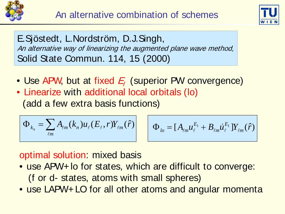
E.Sjöstedt, L.Nordström, D.J.Singh,An alternative way of linearizing the augmented plane wave method,Solid State Commun. 114, 15 (2000)
• Use APW, but at fixed El (superior PW convergence)• Linearize with additional local orbitals (lo)(add a few extra basis functions)
)ˆ(][ 11 rYuBuA mE
mE
mlo +=Φ
optimal solution: mixed basis• use APW+lo for states, which are difficult to converge:
(f or d- states, atoms with small spheres)• use LAPW+LO for all other atoms and angular momenta

Improved convergence of APW+lo
e.g. force (Fy) on oxygen in SES
vs. # plane waves: in LAPW changes sign
and converges slowly in APW+lo better
convergence to same value as in LAPW
SES (sodium electro solodalite)
K.Schwarz, P.Blaha, G.K.H.Madsen,Comp.Phys.Commun.147, 71-76 (2002)
Representative Convergence:
SES
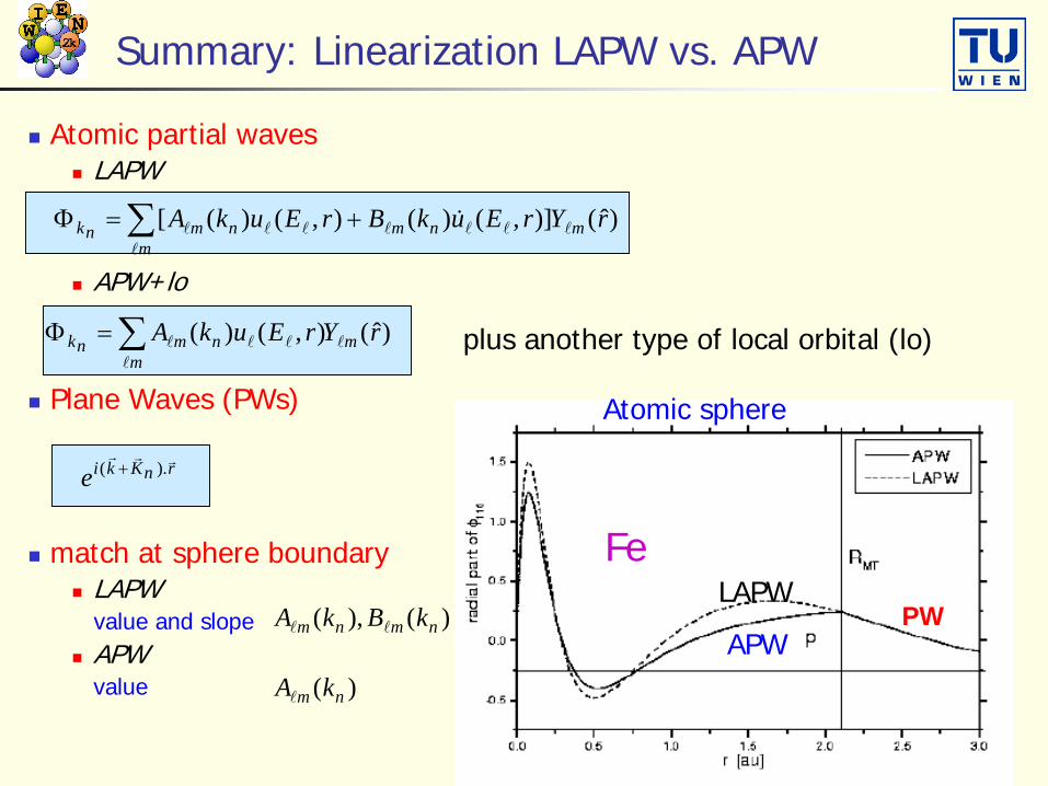
Summary: Linearization LAPW vs. APW
Atomic partial waves LAPW
APW+lo
Plane Waves (PWs)
match at sphere boundary LAPW
value and slope APW
value
)ˆ()],()(),()([ rYrEukBrEukA mnm
mnmnk
∑ +=Φ
rnKkie
).( +
)ˆ(),()( rYrEukA mm
nmnk
∑=Φ
)( nm kA
)(),( nmnm kBkA
Atomic sphere
PW
plus another type of local orbital (lo)
LAPW
APW
Fe

Method implemented in WIEN2k
E.Sjöststedt, L.Nordström, D.J.Singh, SSC 114, 15 (2000)
• Use APW, but at fixed El (superior PW convergence)• Linearize with additional lo (add a few basis functions)
optimal solution: mixed basis• use APW+lo for states which are difficult to converge: (f- or d- states, atoms with small spheres)
• use LAPW+LO for all other atoms and angular momenta
K.Schwarz, P.Blaha, G.K.H.Madsen,Comp.Phys.Commun.147, 71-76 (2002)
A summary is given in

The WIEN2k authors
G.MadsenP.Blaha
D.KvasnickaK.Schwarz
J.Luitz
An Augmented Plane Wave Plus Local Orbital Program for Calculating Crystal Properties
Peter BlahaKarlheinz Schwarz
Georg MadsenDieter Kvasnicka
Joachim Luitz
November 2001Vienna, AUSTRIA
Vienna University of Technology http://www.wien2k.at

International users
about 2500 licenses worldwide
75 industries (Canon, Eastman, Exxon, Fuji, Hitachi, IBM, Idemitsu Petrochem., Kansai, Komatsu, Konica-Minolta, A.D.Little, Mitsubishi, Mitsui Mining, Motorola, NEC, Nippon Steel, Norsk Hydro, Osram, Panasonic, Samsung, Seiko Epson, Siemens, Sony, Sumitomo,TDK,Toyota).
Europe: A, B, CH, CZ, D, DK, ES, F, FIN, GR, H, I, IL, IRE, N, NL, PL, RO, S, SK, SL, SI, UK (ETH Zürich, MPI Stuttgart, FHI Berlin, DESY, RWTH Aachen, ESRF, Prague, IJS Ljubjlana, Paris, Chalmers, Cambridge, Oxford)
America: ARG, BZ, CDN, MX, USA (MIT, NIST, Berkeley, Princeton, Harvard, Argonne NL, Los Alamos NL, Oak Ridge NL, Penn State, Purdue, Georgia Tech, Lehigh, John Hopkins, Chicago, Stony Brook, SUNY, UC St.Barbara, UCLA)
far east: AUS, China, India, JPN, Korea, Pakistan, Singapore,Taiwan (Beijing, Tokyo, Osaka, Kyoto, Sendai, Tsukuba, Hong Kong)
mailinglist: 10.000 emails/6 years

The first publication of the WIEN code

Europa Austria Vienna WIEN
In the Heart of EUROPE
AustriaVienna
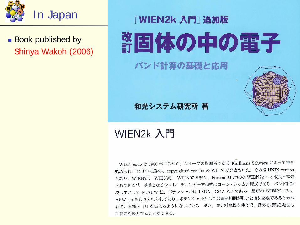
In Japan
Book published byShinya Wakoh (2006)

Development of WIEN2k Authors of WIEN2k
P. Blaha, K. Schwarz, D. Kvasnicka, G. Madsen and J. Luitz Other contributions to WIEN2k
C. Ambrosch-Draxl (Univ. Graz, Austria), optics E. Assmann (Vienna) Wannier functions F. Karsai (Vienna) parallelization R. Laskowski (Singapore), non-collinear magnetism, NMR chemical shifts, BSE L. Marks (Northwestern, US) , various optimizations, new mixer P. Novák and J. Kunes (Prague), LDA+U, SO B. Olejnik (Vienna), non-linear optics, C. Persson (Uppsala), irreducible representations V. Petricek (Prague) 230 space groups O. Rubel (Lakehead) Berry phases M. Scheffler (Fritz Haber Inst., Berlin), forces D.J.Singh (NRL, Washington D.C., Oak Ridge), local oribtals (LO), APW+lo E. Sjöstedt and L Nordström (Uppsala, Sweden), APW+lo J. Sofo (Penn State, USA) and J. Fuhr (Barriloche), Bader analysis F. Tran (Vienna) Hartree Fock, DFT functionals B. Yanchitsky and A. Timoshevskii (Kiev), space group
and many others ….
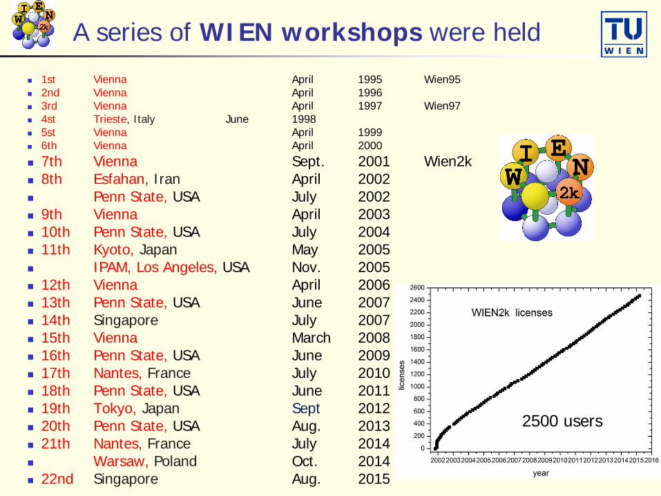
A series of WIEN workshops were held
1st Vienna April 1995 Wien95 2nd Vienna April 1996 3rd Vienna April 1997 Wien97 4st Trieste, Italy June 1998 5st Vienna April 1999 6th Vienna April 2000 7th Vienna Sept. 2001 Wien2k 8th Esfahan, Iran April 2002 Penn State, USA July 2002 9th Vienna April 2003 10th Penn State, USA July 2004 11th Kyoto, Japan May 2005 IPAM, Los Angeles, USA Nov. 2005 12th Vienna April 2006 13th Penn State, USA June 2007 14th Singapore July 2007 15th Vienna March 2008 16th Penn State, USA June 2009 17th Nantes, France July 2010 18th Penn State, USA June 2011 19th Tokyo, Japan Sept 2012 20th Penn State, USA Aug. 2013 21th Nantes, France July 2014 Warsaw, Poland Oct. 2014 22nd Singapore Aug. 2015
2500 users
(L)APW methods
kkK
k nn
n
C = φ∑Ψ
spin polarization shift of d-bands
Lower Hubbard band (spin up)
Upper Hubbard band (spin down)
0 = C
>E<
>|<
>|H|< = >E<
k nδ
δ
ΨΨ
ΨΨ
kkK
k nn
n
C = φ∑Ψ
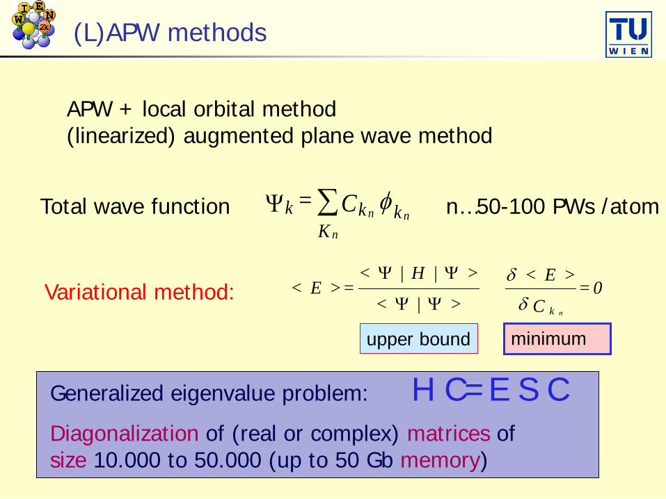
APW + local orbital method (linearized) augmented plane wave method
Total wave function n…50-100 PWs /atom
Variational method:
Generalized eigenvalue problem: H C=E S CDiagonalization of (real or complex) matrices of size 10.000 to 50.000 (up to 50 Gb memory)
upper bound minimum
Structure: a,b,c,α,β,γ, Rα , ...
Ei+1-Ei < ε
Etot, force
Minimize E, force→0
properties
yes
V(ρ) = VC+Vxc Poisson, DFT
DFT Kohn-Sham
Structure optimization
iteration i
no
SCF
k ∈ IBZ (irred.Brillouin zone)
kkk EV ψψρ =+−∇ )]([ 2Kohn Sham
∑ Φ=nk
nknkk Cψ
Variational method 0=><nkC
Eδδ
Generalized eigenvalue problem
ESCHC =
∑≤
=FEkE
kk ψψρ *
k
unit cell atomic positionsk-mesh in reciprocal space

The Brillouin zone (BZ)
Irreducible BZ (IBZ) The irreducible wedge Region, from which the
whole BZ can be obtained by applying all symmetry operations
Bilbao Crystallographic Server: www.cryst.ehu.es/cryst/ The IBZ of all space groups
can be obtained from this server
using the option KVEC and specifying the space group (e.g. No.225 for the fcc structure leading to bcc in reciprocal space, No.229 )
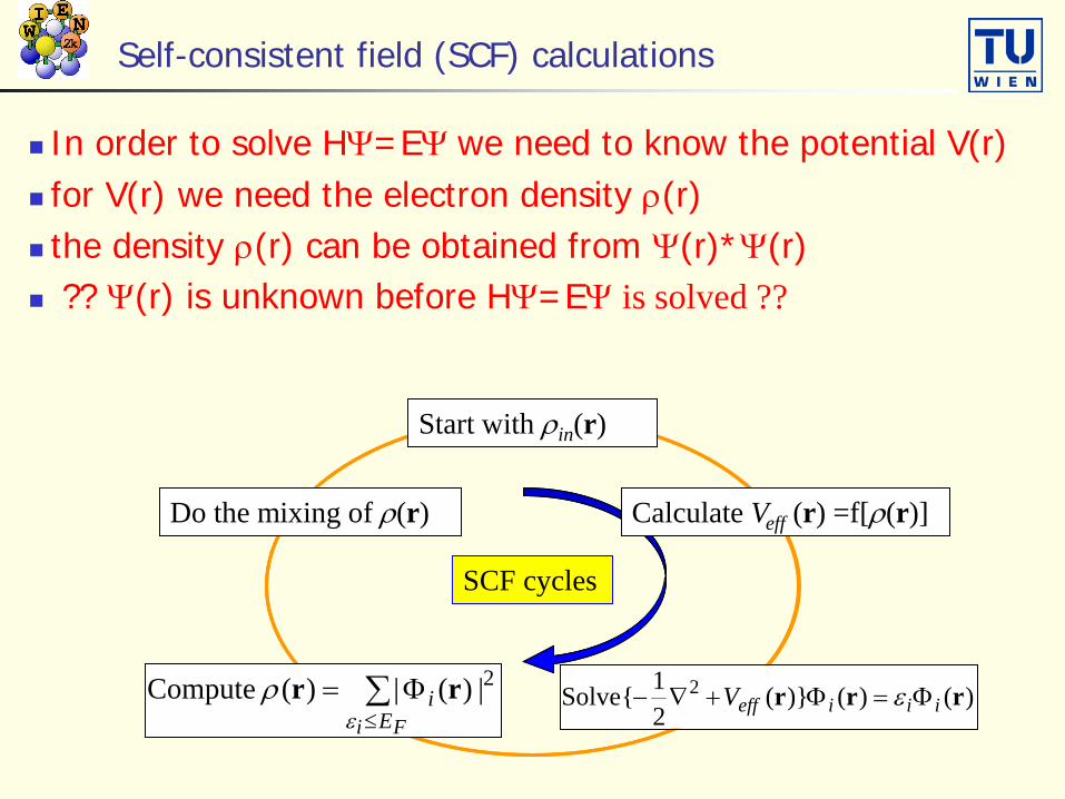
Self-consistent field (SCF) calculations
In order to solve HΨ=EΨ we need to know the potential V(r) for V(r) we need the electron density ρ(r) the density ρ(r) can be obtained from Ψ(r)*Ψ(r) ?? Ψ(r) is unknown before HΨ=EΨ is solved ??
SCF cycles
Start with ρin(r)
Calculate Veff (r) =f[ρ(r)]
)()()}(21{Solve 2 rrr iiieffV Φ=Φ+∇− ε∑
≤Φ=
Fi Ei
ερ 2|)(|)(Compute rr
Do the mixing of ρ(r)
SCF cycles
Start with ρin(r)
Calculate Veff (r) =f[ρ(r)]
)()()}(21{Solve 2 rrr iiieffV Φ=Φ+∇− ε∑
≤Φ=
Fi Ei
ερ 2|)(|)(Compute rr
Do the mixing of ρ(r)

Effects of SCF
Band structure of fcc Cu

Program structure of WIEN2k
init_lapw initialization symmetry detection (F, I, C-
centering, inversion) input generation with
recommended defaults quality (and computing time)
depends on k-mesh and R.Kmax (determines #PW)
run_lapw scf-cycle optional with SO and/or LDA+U different convergence criteria
(energy, charge, forces) save_lapw tic_gga_100k_rk7_vol0
cp case.struct and clmsum files, mv case.scf file rm case.broyd* files

Flow Chart of WIEN2k (SCF)
converged?
Input ρn-1(r)
lapw0: calculates V(r)
lapw1: sets up H and S and solves the generalized eigenvalue problem
lapw2: computes the valence charge density
no yesdone!
lcore
mixer
WIEN2k: P. Blaha, K. Schwarz, G. Madsen, D. Kvasnicka, and J. Luitz
Vorführender
Präsentationsnotizen
Um zu veranschaulichen, wie so eine Rechnung abläuft habe ich hier ein Flussdiagramm skizziert Geeignete Startladungsdichte: Superposition/Überlagerung aus atomaren Dichten Aus der Ladungsdichte wird das Potential konstruiert und zwar Vhartree Lsg der Poisson Gl. Im Zwischenbereich dank Pseudoladungsmethode im reziproken Raum In den MTs Randwertproblem aus der Bedingung der Stetigkeit des Potentials am Sphärenrand Danach werden H und S in der Basis aufgestellt und das verallg. EW Problem gelöst. Dies ist meist der zeitaufwendigste Schritt. Danach wird aus den WF die neue Ladungsdichte berechnet und mit der Information aus vorigen Iterationen die neue Ladungsdichte erzeugt.

Workflow of a WIEN2k calculation
• individual FORTRAN programs linked by shell-scripts• the output of one program is input for the next• lapw1/2 can run in parallel on many processors
LAPW0
LAPW1
LAPW2
LCORE
LAPW0
LCORE
MIXER
SUMPARA
LAPW1
LAPW2
SCF cycle
single mode parallel mode
Iter
atio
n Iter
atio
n
75 %
20 %
3 %*
1%
1%
selfconsistent? ENDyesno
MIXER
selfconsistent?END yes no
k-point parallelization
* fraction of total computation time
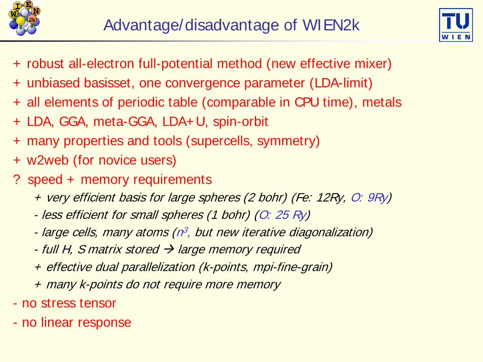
Advantage/disadvantage of WIEN2k
+ robust all-electron full-potential method (new effective mixer)+ unbiased basisset, one convergence parameter (LDA-limit)+ all elements of periodic table (comparable in CPU time), metals+ LDA, GGA, meta-GGA, LDA+U, spin-orbit+ many properties and tools (supercells, symmetry)+ w2web (for novice users)? speed + memory requirements
+ very efficient basis for large spheres (2 bohr) (Fe: 12Ry, O: 9Ry)- less efficient for small spheres (1 bohr) (O: 25 Ry)- large cells, many atoms (n3, but new iterative diagonalization)- full H, S matrix stored large memory required+ effective dual parallelization (k-points, mpi-fine-grain)+ many k-points do not require more memory
- no stress tensor- no linear response

w2web GUI (graphical user interface)
Structure generator spacegroup selection import cif file
step by step initialization symmetry detection automatic input generation
SCF calculations Magnetism (spin-polarization) Spin-orbit coupling Forces (automatic geometry
optimization) Guided Tasks
Energy band structure DOS Electron density X-ray spectra Optics

Structure given by:spacegrouplattice parameterpositions of atoms(basis)
Rutile TiO2:P42/mnm (136)a=8.68, c=5.59 bohrTi: (0,0,0)
O: (0.304,0.304,0)Wyckoff position: x, x, 0
Spacegroup P42/mnm
2a
4f
TiO

Quantum mechanics at work
thanks to Erich Wimmer

TiC electron density
NaCl structure (100) plane Valence electrons only plot in 2 dimensions Shows
charge distribution covalent bonding
between the Ti-3d and C-2p electrons
eg/t2g symmetry
CTi
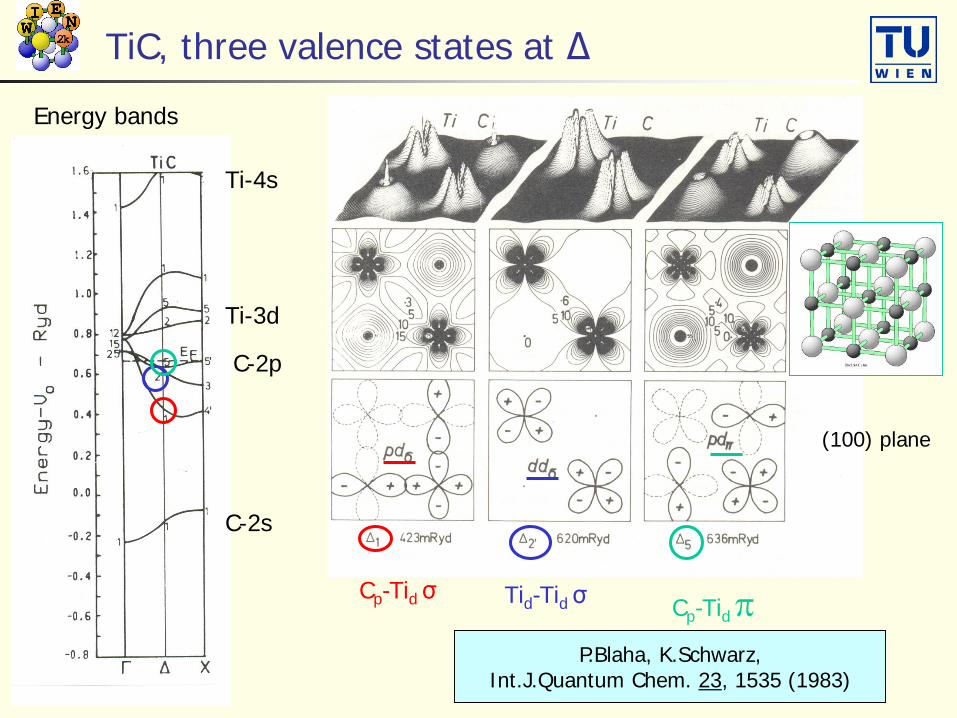
TiC, three valence states at Δ
Energy bands
C-2p
C-2s
Ti-3d
Ti-4s
Cp-Tid σ Tid-Tid σ Cp-Tid πP.Blaha, K.Schwarz,
Int.J.Quantum Chem. 23, 1535 (1983)
(100) plane

TiC, energy bands
P.Blaha, K.Schwarz,Int.J.Quantum Chem. 23, 1535 (1983)
spaghetti irred.rep. character bands

TiC, bonding and antibonding states
P.Blaha, K.Schwarz,Int.J.Quantum Chem. 23, 1535 (1983)
C-2p
O-2p
Ti-3d
bonding
antibonding
weight: C TiO Ti
C-2s
O-2s

Bonding and antibondig state at Δ1
antibondingCp-Tid σ
bondingCp-Tid σ

TiC, TiN, TiO
P.Blaha, K.Schwarz,Int.J.Quantum Chem. 23, 1535 (1983)
Rigid band model: limitations
TiC TiN TiO
Electron density ρ: decomposition
unit cell interstitial atom t ℓ=s, p, d, …
∑∑+=
tt
out qq1
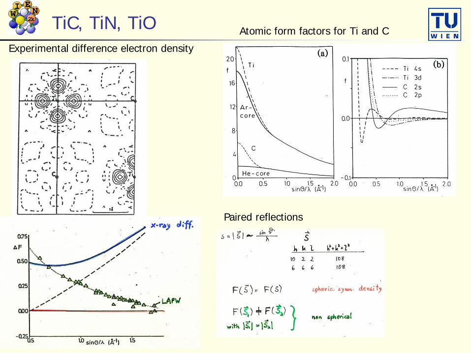
TiC, TiN, TiO Atomic form factors for Ti and C
Paired reflections
Experimental difference electron density

Crucial aspects for a simulation
These aspects need to be considered when comparing theory with experiment.
stoichiometry electron core-hole vacuum average disorder satellites supercell vibrations impurities, defects all electron ℓ quantum n.
Theory vs. experiment: Agreement or disagreement: What can cause it?
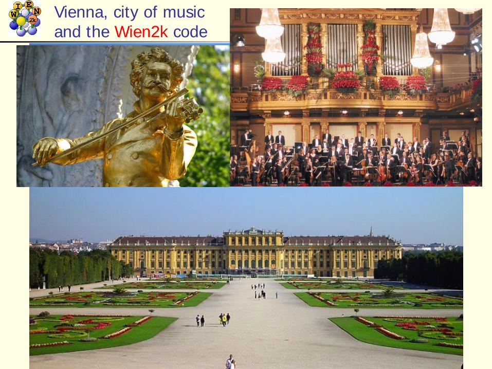
Vienna, city of music and the Wien2k code


![PUBLISHED VERSION Constrained density functional for ... · Althoughabinitiocalculationsoftenassumecollinearmag-netic configurations, spin-polarized density functional theory (DFT)[20]doesnotimposeanyconstraintsonthedirectionsof](https://static.fdocuments.in/doc/165x107/5b4935857f8b9a3a058d522d/published-version-constrained-density-functional-for-althoughabinitiocalculationsoftenassumecollinearmag-netic.jpg)