Density functional studies of the electronic structure and ...
99
Density functional studies of the electronic structure and transport properties of thermoelectric materials Espen Flage-Larsen Thesis submitted in partial fulfillment of the requirements for the degree of Philosophiae Doctor Department of Physics University of Oslo August 2009
Transcript of Density functional studies of the electronic structure and ...

Density functional studies of the electronicstructure and transport properties of
thermoelectric materials
Espen Flage-Larsen
Thesis submitted in partial fulfillmentof the requirements for the degree of
Philosophiae Doctor
Department of PhysicsUniversity of Oslo
August 2009
© Espen Flage-Larsen, 2009 Series of dissertations submitted to the Faculty of Mathematics and Natural Sciences, University of Oslo No. 906 ISSN 1501-7710 All rights reserved. No part of this publication may be reproduced or transmitted, in any form or by any means, without permission. Cover: Inger Sandved Anfinsen. Printed in Norway: AiT e-dit AS, Oslo, 2009. Produced in co-operation with Unipub AS. The thesis is produced by Unipub AS merely in connection with the thesis defence. Kindly direct all inquiries regarding the thesis to the copyright holder or the unit which grants the doctorate. Unipub AS is owned by The University Foundation for Student Life (SiO)

Summary
The present work was set to study materials, and in particular thermoelectric materials basedon first–principle calculations. Density functional theory was used to calculate the electronicstructure of skutterudites, Zintl compounds and black phosphorus. Transport properties can beobtained experimentally, but routines for calculating these from first–principles have not beenfully developed. Thus, much effort was put into the development, implementation and testingof routines that calculate transport properties based on the electronic structure. Electron transferanalyses were also performed for selected skutterudites and Zintl compounds to explicitly inves-tigate their bonds. The combination of experimental and theoretical studies is mutually beneficialand wherever possible experimental data have been included to verify or further investigate theelectronic structure and transport properties.

Acknowledgements
I would like to express gratitude to my supervisors, Johan Taftø and Ole Martin Løvvik for theirencouragement, scientific knowledge, enthusiasm and kindness during my three years of workon this thesis. I also appreciate countless hours of discussions with Øystein Prytz, Ole BjørnKarlsen and Simone Casolo, both on a scientific and personal level. In addition, Spyros Diplas,Terje Finstad, Kjetil Valset, Michael Bottger, Lars–Olav Vestland and Protima Rauwel deservethanks for their scientific interest.
Georg Kresse, Judith Harl and the rest of the people in the VASP group in Vienna should bethanked for their knowledge, support and kindness during my visits.
During my stay at Caltech, Jeff Snyder, Eric Toberer, Andrew May, Yanzhong Pei and AliSaramat should be acknowledged for excellent hospitality and great discussions.
I would also like to express my deepest gratitude and love to my family for their everlastingsupport and understanding. They early inspired the need of curiosity and dedication in every-day life, factors I strongly feel have been major contributors to this thesis. And aside from thescientific aspects, their personal support has always been unsurpassed.
Finally, I would like to thank the Norwegian Research Council for financial support and theNOTUR project for computational resources.
Espen Flage–Larsen, 2009

Preface
This thesis was developed for the partial fulfilment of the requirements for the degree of PhilosophiaeDoctor at the University of Oslo. All work was funded by the Norwegian Research councilthrough the project “Studies of the electronic structure of materials at the nanoscale”. The workstarted autumn 2006 and ended three years later.
The title of the thesis is “Density functional studies of the electronic structure and trans-port properties of thermoelectric materials”, a title that mainly describes its contents. However,even though this work is biased towards theory, focus incorporating experiments has been im-portant for the published work. The author is a strong believer of the importance of an increasedcollaboration between experiment and theory.
Several visits to the VASP group in Vienna were done, where we worked out and investi-gated different ways of calculating the transport properties based on the VASP density functionalengine.
Spring 2009 was spent at Jeff Snyder’s thermoelectrics group at California Institute of Tech-nology, where the author assisted Jeff Snyder, Eric Toberer and Andrew May with density func-tional and first–principle transport calculations.


Table of Contents
Summary 3
Acknowledgements 5
Preface 7
Table of Contents 9
1 Introduction 13Bibliography . . . . . . . . . . . . . . . . . . . . . . . . . . . . . . . . . . . . . . . 16References . . . . . . . . . . . . . . . . . . . . . . . . . . . . . . . . . . . . . . . . . 16
2 Thermoelectricity 172.1 Basic principles . . . . . . . . . . . . . . . . . . . . . . . . . . . . . . . . . . . 18
2.1.1 Seebeck effect . . . . . . . . . . . . . . . . . . . . . . . . . . . . . . . 182.1.2 Peltier effect . . . . . . . . . . . . . . . . . . . . . . . . . . . . . . . . 182.1.3 Thomson effect . . . . . . . . . . . . . . . . . . . . . . . . . . . . . . . 182.1.4 Figure of merit . . . . . . . . . . . . . . . . . . . . . . . . . . . . . . . 19
2.2 Thermoelectric device . . . . . . . . . . . . . . . . . . . . . . . . . . . . . . . . 192.3 Current and future status . . . . . . . . . . . . . . . . . . . . . . . . . . . . . . 19
2.3.1 Typical materials . . . . . . . . . . . . . . . . . . . . . . . . . . . . . . 192.3.2 Current fields of application . . . . . . . . . . . . . . . . . . . . . . . . 202.3.3 Future applications . . . . . . . . . . . . . . . . . . . . . . . . . . . . . 23
References . . . . . . . . . . . . . . . . . . . . . . . . . . . . . . . . . . . . . . . . . 25
3 Density functional theory studies of thermoelectric materials 273.1 Ab–initio solutions of the Schrodinger equation . . . . . . . . . . . . . . . . . . 273.2 Density functional theory . . . . . . . . . . . . . . . . . . . . . . . . . . . . . . 29

10 Table of Contents
3.2.1 Basics . . . . . . . . . . . . . . . . . . . . . . . . . . . . . . . . . . . . 293.2.2 Choice of basis set . . . . . . . . . . . . . . . . . . . . . . . . . . . . . 343.2.3 Exchange–correlation functionals . . . . . . . . . . . . . . . . . . . . . 37
3.3 Electronic structure and bonding . . . . . . . . . . . . . . . . . . . . . . . . . . 413.3.1 Electron density analysis . . . . . . . . . . . . . . . . . . . . . . . . . . 413.3.2 A few examples . . . . . . . . . . . . . . . . . . . . . . . . . . . . . . . 42
3.4 Transport properties . . . . . . . . . . . . . . . . . . . . . . . . . . . . . . . . . 473.4.1 Electronic transport in solids . . . . . . . . . . . . . . . . . . . . . . . . 473.4.2 The Boltzmann equation . . . . . . . . . . . . . . . . . . . . . . . . . . 503.4.3 Non–equilibrium distribution function . . . . . . . . . . . . . . . . . . . 513.4.4 The Boltzmann transport equations . . . . . . . . . . . . . . . . . . . . 543.4.5 Implementation . . . . . . . . . . . . . . . . . . . . . . . . . . . . . . . 57
3.5 Band engineering and the impact on the transport properties . . . . . . . . . . . 663.5.1 Chemical potential or carrier concentration . . . . . . . . . . . . . . . . 703.5.2 Temperature . . . . . . . . . . . . . . . . . . . . . . . . . . . . . . . . 713.5.3 Curvature . . . . . . . . . . . . . . . . . . . . . . . . . . . . . . . . . . 723.5.4 Degeneracy and reciprocal shift . . . . . . . . . . . . . . . . . . . . . . 733.5.5 Energy shift . . . . . . . . . . . . . . . . . . . . . . . . . . . . . . . . . 743.5.6 Conduction band . . . . . . . . . . . . . . . . . . . . . . . . . . . . . . 753.5.7 Modifications due to electron scattering . . . . . . . . . . . . . . . . . . 763.5.8 Power factor and optimization of electronic properties . . . . . . . . . . 793.5.9 Figure–of–merit . . . . . . . . . . . . . . . . . . . . . . . . . . . . . . 813.5.10 Energy filtering . . . . . . . . . . . . . . . . . . . . . . . . . . . . . . . 833.5.11 Band structure requirements . . . . . . . . . . . . . . . . . . . . . . . . 85
References . . . . . . . . . . . . . . . . . . . . . . . . . . . . . . . . . . . . . . . . . 89
Paper ITitle: Bond analysis of phosphorus skutterudites: elongated lanthanum electron buildupin LaFe4P12
Authors: E. Flage–Larsen, O. M. Løvvik, Ø. Prytz and J. TaftøStatus: Submitted to Computational Material Science 29.06.2009 95
Paper IITitle: The influence of exact exchange corrections in van der Waals layered narrow bandgap black phosphorus

Table of Contents 11
Authors: Ø. Prytz and E. Flage–LarsenStatus: Submitted to Journal of Physics: Condensed Matter, 11.08.2009 111
Paper IIITitle: Electron energy loss spectroscopy of the L2,3 edge of phosphorus skutterudites andelectronic structure calculationsAuthors: R. Sæterli, E. Flage–Larsen, Ø. Prytz, J. Taftø, K. Marthinsen and R. HolmestadStatus: Accepted in Physical Review B 09.07.2009 129
Paper IVTitle: Electronic structure and transport in thermoelectric compounds AZn2Sb2
(A = Sr, Ca, Yb, Eu)Authors: E. S. Toberer, A. F. May, B. Melot, E. Flage–Larsen and G. J. SnyderStatus: Submitted to Dalton Transactions 14.07.2009 139
Paper VTitle: Valence band study of thermoelectric Zintl SrZn2Sb2 and YbZn2Sb2
Authors: E. Flage–Larsen, S. Diplas, E. S. Toberer and A. F. MayStatus: Submitted to Physical Review B, 12.08.2009 157


Chapter 1
Introduction
Conflicts related both directly and indirectly to energy demands are escalating all over the world.A primary concern for developing nations is to obtain long–term sustainable energy resourceswith as little investment as possible. On the other hand, OECD nations are constantly seekingcontinuity and increased harvest of established energy resources. Naturally, due to the sharedresources, this leads, and will lead to local and global conflicts. Environmental concerns are alsobecoming more important due to increased emissions from fossil fuels, nuclear waste and localhavoc of natural habitats of animals and plants.
Today’s global energy consumption is estimated to be close to 500 quadrillion BTU (BritishThermal Unit) (see Fig. 1.1). Extrapolation surveys from Energy Information Administration(EIA) [1] show that the world’s total energy demands are expected to soar by 44% by 2030 (seeFig. 1.1), much due to economic growth in the developing nations. The OECD nations accountfor the largest share of today’s energy consumption. However, as Fig. 1.1 indicates, this is aboutto change due to the rapid growth of energy demand in the developing nations, in particularChina.
The dominating energy resource is still expected to be liquid (fossil fuels and bio fuels) andit is increasing steadily each year. Coal and renewable energy resources increase the most. Thesesurveys are based on a relatively high fuel cost and thus any unforeseen change would likely yielda different distribution among the energy resources. Even though the transport sector is highlydependent on liquid fuels, we see from Fig. 1.2 that the future increase of energy consumptionis mostly due to demand for electricity, where the largest contributors are the Asian nations. Itis also interesting to note the projected distribution among the renewable energy resources inFig. 1.2, where the hydroelectricity now dominates, surpassed in 2030 by the rapid increase ofwind energy. The share of the other renewable energy resources are almost an order of magnitude

14 Chapter 1. Introduction
200300400500 OECD
non-OECD
75150225300
Ener
gy c
onsu
mpt
ion
[Qua
drill
ion
BTU
]
LiquidsNatural gasCoalNuclearRenewables
1980 1990 2000 2010 2020 2030Year
255075
100 ChinaIndiaUnited StatesRest of the world
Figure 1.1: The world’s energy consumption from 1980 to 2030. Top figure shows OECD andnon–OECD energy consumption. The total energy consumption is split into different energyresources in the middle figure, while the lower figure shows a more detailed comparison of thenations’ energy consumption. Data from International Energy Outlook 2009, EIA [1].
10203040 OECD
Non-OECDTotal electricityTotal energy
48
1216
Ener
gy c
onsu
mpt
ion
[Tril
lion
kWh]
non-OECD AsiaNon-OECD E. Eu.Middle EastAfricaC. and S. America
1980 1990 2000 2010 2020 2030Year
0.2
0.4
0.6
0.8 Other renewablesHydroelectricityWindGeothermal
Figure 1.2: The world’s net electricity generation from 1980 to 2030. Top figure comparesOECD, non–OECD electricity generation and the total energy consumption to the total electricitygeneration. Middle figure splits the electricity generation into different continents, while thelower figure gives estimates of the OECD Europe nations’ renewable electricity generation. Datafrom International Energy Outlook 2009, EIA [1]

15
Figure 1.3: United States electricity generation, transmission and energy loss. Figure fromLawrence Livermore National Laboratory [2].
smaller.Extensive research efforts have been put into traditional energy fields like nuclear, thermal
and water energy. In parallel there has been inclining interest in alternative resources, suchas solar, wind and ocean wave energy. Most of these energy fields are based on first stageenergy exploitation, where the base energy is available in nature. However, second stage energyexploitation is also possible by collecting waste heat from a primary process and then convertthis to a given form of distributable energy. The energy loss of different processes is illustratedin Fig. 1.3, where it is clear that over 50% of the total energy harvest potential is lost to wasteheat. The potential to exploit heat from factories, power plants, cars, tumble driers, electroniccircuits and so forth is thus astonishingly large.
Thermoelectricity is a particular interesting solid–state alternative for converting heat to elec-tricity. Although it can be used on a primary energy source, it is thought to be even more usefulin a secondary stage to collect waste heat. Without the need of moving parts, the longevity andadaptability are expected to be excellent. An additional benefit is flexibility, due to the dual na-ture of the thermoelectric device, which by reversing the voltage can operate both as a heaterand a cooler. Simultaneously, waste heat conversion can be exploited in the same device. Unfor-
16 Chapter 1. Introduction
tunately, the thermoelectric materials used in an assembled thermoelectric device are currentlytoo inefficient to compete with traditional heat conversion cycles. However, comprehensive im-provements are expected once a more complete understanding of the physics and chemistry ofthese materials is achieved.
Motivated by this, we in this work, try to develop a more solid footing for first–principlecalculations of materials and in particular, thermoelectric materials. We have tried to keep thiswork consistent and in close collaboration with experiments and believe this is crucial to ob-tain breakthroughs in this field. Readers are encouraged to consult the bibliography for moreextensive background information.
Bibliography
Thermoelectrics Handbook, edited by D. M. Rowe, CRC, Boca Raton, 2006Solid State Physics, N. W. Ashcroft and N. D. Mermin, Brooks Cole, 1976Fundamentals of Semiconductors, P. Y. Yu and M. Cardona, Third edition, Springer-Verlag,Berlin, 2001Introduction to Solid State Physics, C. Kittel, Seventh edition, John Wiley & Sons, 1996Density-Functional Theory of Atoms and Molecules, R. G. Parr and W. Yang, Oxford UniversityPress, New York, 1989Density Functional Theory, R. Dreizler and E. Gross, Plenum Press, New York, 1995Density Functional Theory, A Practical Introduction, D. Sholl and J. A. Steckel, John Wiley &Sons, New Jersey, 2009
References
[1] International Energy Outlook 2009, http://eia.doe.gov.
[2] Electricity Generation, Transmission, and Distribution Losses, https://eed.llnl.gov/flow/.

Chapter 2
Thermoelectricity
Simply put, thermoelectricity relates thermal gradients and electrical currents in materials. Throughthis relation it is possible to convert heat to electricity or use electricity for heating or cooling.
The basic principles of thermoelectricity was discovered two centuries ago, however, due tothe lack of understanding of the physical properties of materials it was not until later that sig-nificant progress was done. During the 60’s and 70’s considerable theoretical and experimentalwork was performed, but it was not before the energy debate was brought to the public duringthe 90’s that the field experienced a rapid expansion of research activities.
Even though basic thermoelectric devices have been operating for decades, serving remotelighthouses, unmanned spacecraft and local cooling, their current efficiency is too mediocre tobe a viable alternative for large scale heat conversion applications. For example, current state ofthe art bulk materials have a figure–of–merit, the factor that determines their efficiency, that isthree to four times too low to compete with traditional refrigerator solutions [1]. However it isbelieved that there is a large potential for optimization.
The main reason for thermoelectric research is due to its unique range of applicability, but inaddition, there is a wealth of exciting general physical phenomena governing these devices andin particular the materials that are not yet fully understood. Hence, they also serve as excellentplatforms for solid–state research.
In this chapter we briefly cover the history, the basics and the future of thermoelectricity.

18 Chapter 2. Thermoelectricity
2.1 Basic principles
2.1.1 Seebeck effect
What we today call the Seebeck effect was discovered in 1823 by Thomas Johann Seebeck.He placed a compass needle close to two dissimilar metals in contact. While heating one ofthe conductors the compass needle deflected and Seebeck correctly thought this was caused bymagnetic fields generated by the temperature difference. However, he quickly discovered throughAmpere’s law that it was a current that generated the magnetic field. He concluded that thiscurrent was generated by the temperature difference between the two conductors. The Seebeckcoefficient α was then defined as the ratio between the induced voltage V and the temperaturedifference ΔT ;
α =V
ΔT. (2.1)
2.1.2 Peltier effect
Based on the discoveries of Seebeck, the watchmaker Jean Charles Athanase Peltier detected acomplementary effect 12 years later. During an experiment he observed local heating when acurrent was passed between two different conductors. He failed to explain the nature of this,but used Seebeck’s discoveries to try to explain the phenomenon. It was not until 1838 thatLenz discovered that heating and cooling in the junction between the two dissimilar metals wasdependent on the current direction. Similar to the Seebeck coefficient, the Peltier coefficient Π
was defined as the ratio between power generated at the metal junction Q and the passing currentI sent through the circuit;
Π =Q
I. (2.2)
2.1.3 Thomson effect
Additional insight was given when William Thomson (Lord Kelvin) discovered a relation be-tween the Peltier and the Seebeck effect. He deduced that
Π = αT, (2.3)
where T is the temperature. In light of this he predicted a third thermoelectric effect, the Thom-son effect, which relates the heating and cooling of a conductor in the presence of a temperature

2.2. Thermoelectric device 19
gradient.
2.1.4 Figure of merit
The figure–of–merit is considered the “goodness” factor of a thermoelectric material and itsdimensionless definition is
zT =α2σ
κT, (2.4)
where σ and κ are the thermal and electrical conductivity, respectively. From this relation itis apparent that to obtain a large zT value, we would need a large Seebeck coefficient, largeelectrical conductivity and at the same time a low thermal conductivity. Beside mechanicalproperties and other manufacturing aspects, the most important property of a thermoelectricmaterial is this zT value. It is common nomenclature to use a large Z for the device and asmall z for the material. Due to the importance of zT we will in Sec. 3.4 further discuss itscomponents in light of different electronic structures.
2.2 Thermoelectric device
To put thermoelectricity to practice a thermoelectric device is needed. Such device consistsof small thermocouples made of thermoelectric materials, preferably materials with the highestpossible zT in the operational temperature range. In addition, there are other factors limiting thechoice of materials, like durability and mechanical issues. For historical reasons these devicesare often called “Peltier elements”. The device is usually constructed of alternating n– and p–type materials, electrically connected in series, while thermally in parallel. In Fig. 2.1 a sketchof a simple one layer thermoelectric device is shown. These devices work on an external loadand generate electricity if a thermal gradient normal to the surface is present. The reverse effectis possible if a current is passed through the device, thus generating a thermal gradient. Thisgradient can then be utilized for heating or cooling.
2.3 Current and future status
2.3.1 Typical materials
To fabricate an efficient thermoelectric device, efficient thermoelectric materials is a prerequi-site. Such materials are not strictly metallic, semiconducting or insulating. As a rule of thumb,

20 Chapter 2. Thermoelectricity
Figure 2.1: A typical (and simple) construction of alternating n– and p–type thermoelectric ma-terials to make a thermoelectric device. The individual parts are connected electrically in seriesand thermally in parallel. Electrical connectors are soldered at the ends. Picture is made byMichael Bottger, Basic and Applied Thermoelectric Initiative (BATE) [2], 2009.
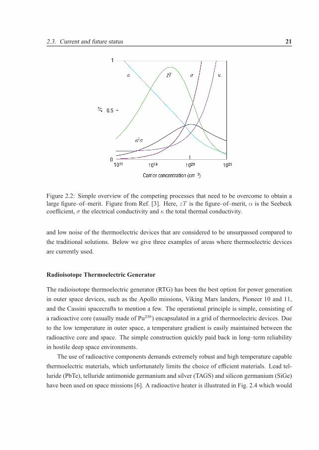
highly doped semiconductors are preferred based on an acceptable balance between the Seebeckcoefficient and the electrical conductivity [3]. In Fig. 2.2 a simplified picture of the competingSeebeck coefficient and the electrical and thermal conductivity are shown. However, it needsto be stressed that this picture is based on simplified models [3]. We will later in this thesis,in Sec. 3.4 discuss band structure properties that give a high zT value (or more specifically itsnumerator). A comparison of the best bulk materials available today is given in Fig. 2.3, but wewould like to emphasize that other promising bulk materials exist as well, such as the AZn2Sb2
compounds (A is rare earth, see Paper IV), the β–Zn4Sb3 [4] compound and the La3Te4 [5]compound to mention a few.
2.3.2 Current fields of application
The efficiency of existing materials is unfortunately too low for widespread applications. Com-pression units (refrigerators, steam engines etc.) are more efficient and it is necessary to sig-nificantly improve the zT value of the materials to make them a viable alternative for largescale applications. In general it is believed that a zT greater than three (currently, the best bulkmaterials have zT ∼ 1, see Fig. 2.3) would be enough to compete with current refrigerator appli-cations [1]. However, even though today’s efficiency is low, there are areas of applications wherethermoelectric devices are (and have been) favourable. This is due to the longevity, ruggedness
2.3. Current and future status 21
Figure 2.2: Simple overview of the competing processes that need to be overcome to obtain alarge figure–of–merit. Figure from Ref. [3]. Here, zT is the figure–of–merit, α is the Seebeckcoefficient, σ the electrical conductivity and κ the total thermal conductivity.
and low noise of the thermoelectric devices that are considered to be unsurpassed compared tothe traditional solutions. Below we give three examples of areas where thermoelectric devicesare currently used.
Radioisotope Thermoelectric Generator
The radioisotope thermoelectric generator (RTG) has been the best option for power generationin outer space devices, such as the Apollo missions, Viking Mars landers, Pioneer 10 and 11,and the Cassini spacecrafts to mention a few. The operational principle is simple, consisting ofa radioactive core (usually made of Pu238) encapsulated in a grid of thermoelectric devices. Dueto the low temperature in outer space, a temperature gradient is easily maintained between theradioactive core and space. The simple construction quickly paid back in long–term reliabilityin hostile deep space environments.
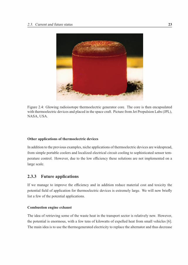
The use of radioactive components demands extremely robust and high temperature capablethermoelectric materials, which unfortunately limits the choice of efficient materials. Lead tel-luride (PbTe), telluride antimonide germanium and silver (TAGS) and silicon germanium (SiGe)have been used on space missions [6]. A radioactive heater is illustrated in Fig. 2.4 which would
22 Chapter 2. Thermoelectricity
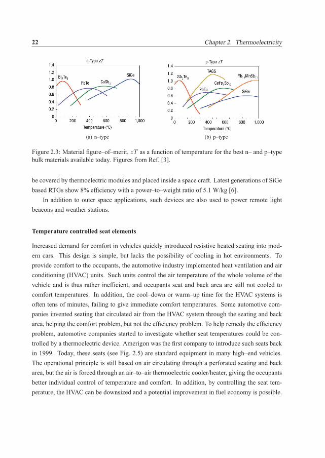
(a) n–type (b) p–type
Figure 2.3: Material figure–of–merit, zT as a function of temperature for the best n– and p–typebulk materials available today. Figures from Ref. [3].
be covered by thermoelectric modules and placed inside a space craft. Latest generations of SiGebased RTGs show 8% efficiency with a power–to–weight ratio of 5.1 W/kg [6].
In addition to outer space applications, such devices are also used to power remote lightbeacons and weather stations.
Temperature controlled seat elements
Increased demand for comfort in vehicles quickly introduced resistive heated seating into mod-ern cars. This design is simple, but lacks the possibility of cooling in hot environments. Toprovide comfort to the occupants, the automotive industry implemented heat ventilation and airconditioning (HVAC) units. Such units control the air temperature of the whole volume of thevehicle and is thus rather inefficient, and occupants seat and back area are still not cooled tocomfort temperatures. In addition, the cool–down or warm–up time for the HVAC systems isoften tens of minutes, failing to give immediate comfort temperatures. Some automotive com-panies invented seating that circulated air from the HVAC system through the seating and backarea, helping the comfort problem, but not the efficiency problem. To help remedy the efficiencyproblem, automotive companies started to investigate whether seat temperatures could be con-trolled by a thermoelectric device. Amerigon was the first company to introduce such seats backin 1999. Today, these seats (see Fig. 2.5) are standard equipment in many high–end vehicles.The operational principle is still based on air circulating through a perforated seating and backarea, but the air is forced through an air–to–air thermoelectric cooler/heater, giving the occupantsbetter individual control of temperature and comfort. In addition, by controlling the seat tem-perature, the HVAC can be downsized and a potential improvement in fuel economy is possible.
2.3. Current and future status 23
Figure 2.4: Glowing radioisotope thermoelectric generator core. The core is then encapsulatedwith thermoelectric devices and placed in the space craft. Picture from Jet Propulsion Labs (JPL),NASA, USA.
Other applications of thermoelectric devices
In addition to the previous examples, niche applications of thermoelectric devices are widespread,from simple portable coolers and localized electrical circuit cooling to sophisticated sensor tem-perature control. However, due to the low efficiency these solutions are not implemented on alarge scale.
2.3.3 Future applications
If we manage to improve the efficiency and in addition reduce material cost and toxicity thepotential field of application for thermoelectric devices is extremely large. We will now brieflylist a few of the potential applications.
Combustion engine exhaust
The idea of retrieving some of the waste heat in the transport sector is relatively new. However,the potential is enormous, with a few tens of kilowatts of expelled heat from small vehicles [6].The main idea is to use the thermogenerated electricity to replace the alternator and thus decrease

24 Chapter 2. Thermoelectricity
Figure 2.5: Climate controlled seating (CCS) from Amerigon. These seats use thermoelectricelements to heat or cool the air that is circulated through perforated leather areas in the cushionand seat back. Picture from Amerigon, USA.
the motor load to improve fuel economy. General Motors, BMW and Fiat have official programsrunning. Prototypes from General Motors have shown that it is possible to decrease the totalfuel consumption by five percent [7]. Even though this number seems relatively small, there isroom for improvements both on the device engineering and the type of materials used. One ofthe first prototypes made for a Chevrolet Suburban is shown in Fig. 2.6. Today they claim 750Wof output power [7] during highway driving.
Other potential applications
Due to the current lack of efficiency, application studies of thermoelectric devices have beenlimited and their potential applications are only briefly mentioned in survey studies. Here welist some applications that might benefit from thermoelectric devices once their efficiency isimproved;
• Three stage solar units. This idea is based on a three stage sandwich design made ofsolar cells followed by thermoelectric elements and then a cooling stage with circulatingwater. In this way, electricity is generated from both the solar cells and the thermoelectricelements, while the facility is heated by the heated circulated water.
• Refrigerator and air conditioner. Thermoelectric elements would increase longevity andreduce noise. Additional benefits are more compact design and better possibilities to tailordesigns to specific needs.

References 25
Figure 2.6: A ten–year old exhaust thermoelectric prototype from General Motors. Picture fromGeneral Motors, USA.
• Embedded heating and cooling. Localized cooling and heating are becoming increasinglyimportant for the semi–conductor industry. Embedded designs would increase stabilityand operational temperature range. Electricity could potentially be harvested from localtemperature gradients.
• Large scale generation of electricity from industrial waste heat.
• Small scale generation of heat and heat conversion in housings.
• Blanket shields for fission (and maybe in the future fusion) plants using thermoelectricdevices to generate electricity from the expelled heat.
• Direct conversion of heat to electricity from furnaces operating a diverse selection of fuels.
References
[1] T. C. Harman, P. J. Taylor, M. P. Walsh, and B. E. LaForge. Quantum dot superlatticethermoelectric materials and devices. Science, 297:2229, 2002.
[2] Basic and Applied Thermoelectric Initiative (BATE), http://www.fys.uio.no/
bate.
26 Chapter 2. Thermoelectricity
[3] G. J. Snyder and E. S. Toberer. Complex thermoelectric materials. Nature Materials, 7:105–114, 2008.
[4] G. J. Snyder, M. Christensen, E. Nishibori, T. Caillat, and B. Brummerstedt Iversen. Dis-ordered zinc in Zn4Sb3 with phonon-glass and electron-crystal thermoelectric properties.Nature Materials, 3:458, 2004.
[5] A. F. May, D. J. Singh, and G. J. Snyder. Influence of band structure on the large thermo-electric performance of lanthanum telluride. Phys. Rev. B, 79:153101, 2009.
[6] J. Yang and T. Caillat. Thermoelectric materials for space and automotive power generation.MRS Bulletin, 31:224, 2006.
[7] Jihui Yang’s talk at MS&T2008 conference in Pittsburgh, US.

Chapter 3
Density functional theory studies ofthermoelectric materials
The core of this thesis is based on density functional theory studies of materials, in particular thethermoelectric branch. Such studies are beneficial since perfect structures can be investigated.This is of great importance due to the complexity of the thermoelectric materials. In addition,once the computational resources permit, large scale simulations can be performed to assist in thesearch for new and promising materials. However, at the same time, density functional studiesare burden by numerous accuracy, performance and general implementation problems.
We will thus devote the first two sections of this chapter to explain the idea and basic prin-ciples behind density functional theory. At the same time we will touch important aspects thatlead to common density functional failures. Then we will move on to a section that covers elec-tron transfer analysis and its use to investigate bonding. Finally, in the last two sections we firstdevelop a way to calculate the transport properties based on the semi–classical Boltzmann equa-tion, and then investigate different band structures and their thermoelectric properties to highlightband structure requirements for good thermoelectric performance.
3.1 Ab–initio solutions of the Schrodinger equation
Basically all non–relativistic quantum mechanical problems boil down to the solution of theSchrodinger equation
H|Ψ〉 = E|Ψ〉, (3.1)
28 Chapter 3. Density functional theory studies of thermoelectric materials
where H, |Ψ〉 and E are the Hamiltonian operator, the eigenvectors (or wavefunctions) and theeigenvalues (or energy levels), respectively. See Ref. [1] (Sec. 6.4) for Dirac notation. Thecomplexity of this equation is well hidden. It can be solved in numerous ways depending on thewanted accuracy and possible ways of formulating the problem.
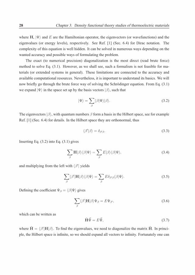
The exact (to numerical precision) diagonalization is the most direct (read brute force)method to solve Eq. (3.1). However, as we shall see, such a formalism is not feasible for ma-terials (or extended systems in general). These limitations are connected to the accuracy andavailable computational resources. Nevertheless, it is important to understand its basics. We willnow briefly go through the brute force way of solving the Schrodinger equation. From Eq. (3.1)we expand |Ψ〉 in the space set up by the basis vectors |β〉, such that
|Ψ〉 =∑
β
〈β|Ψ〉|β〉. (3.2)
The eigenvectors |β〉, with quantum numbers β form a basis in the Hilbert space, see for exampleRef. [1] (Sec. 6.4) for details. In the Hilbert space they are orthonormal, thus
〈β′|β〉 = δβ′β. (3.3)
Inserting Eq. (3.2) into Eq. (3.1) gives
∑β
H|β〉〈β|Ψ〉 =∑
β
E|β〉〈β|Ψ〉, (3.4)
and multiplying from the left with 〈β′| yields
∑β
〈β′|H|β〉〈β|Ψ〉 =∑
β
Eδβ′β〈β|Ψ〉. (3.5)
Defining the coefficient Ψβ = 〈β|Ψ〉 gives
∑β
〈β′|H|β〉Ψβ = EΨβ′ , (3.6)
which can be written asH�Ψ = E�Ψ, (3.7)
where H = 〈β′|H|β〉. To find the eigenvalues, we need to diagonalize the matrix H. In princi-ple, the Hilbert space is infinite, so we should expand all vectors to infinity. Fortunately one can

3.2. Density functional theory 29
introduce a cutoff of the expansion. Such cutoffs are a crucial convergence parameter for exactdiagonalization methods. The diagonalization is usually done by the use of orthogonal transfor-mations. Common procedures for this are the QR algorithm with implicit shifts, Householderreduction and Lanczos algorithm. They are among the most effective methods for solving eigen-problems. The derivation of these methods is outlined in Ref. [2] (Sec. 11.3) and [3] (Sec. 1.1 fora short introduction). To solve the Schrodinger equation, a proper basis and Hamiltonian opera-tor are needed. For many–particle interactions these are not trivial to formulate due to efficiencyand accuracy difficulties. Even though most of these difficulties can be controlled, there is anadditional fundamental problem with the exact diagonalization approach; the eigenvectors fromEq. (3.1) contain all degrees of freedom. Hence, for a n particle system
〈x1x2 . . . xn|Ψ〉 = Ψ(x1, x2, . . . , xn), (3.8)
where xi = {�ri, �si}, the spatial coordinate vector �ri and spin vector �si for particle i. Sucheigenstates would require a huge parameter space. For the spatial part, the parameter spacescales as 3n. It is not uncommon in (even not very complex) materials to handle several hundredparticles. Hence, such a parameter space is unsolvable (regardless of method). We have tointroduce approximations.
3.2 Density functional theory
The idea behind density functional theory (DFT) is to reduce the parameter space. This is doneby posing the problem as a function of the particle density, not the spatial and spin coordinates.Instead of handling a spatial 3n parameter space, we now have a three dimensional parameterspace (or six with spin degrees of freedom), which in principle is computationally constant in n.In this section we will briefly cover the basics of DFT and touch a few topics that are importantfor its practical applications.
3.2.1 Basics
The era of DFT started in 1964 when Hohenberg and Kohn published a paper about a possibleway of solving the interacting electron gas system [4]. We will in this section partly followthis and the additional paper by Kohn and Sham [5]. Hohenberg and Kohn considered a set ofenclosed particles moving in an average background potential Vext(�r) and posed the followingtwo theorems

30 Chapter 3. Density functional theory studies of thermoelectric materials
Theorem 1. The external potential Vext(�r) is (to within a constant) a unique functional of theelectron density n(�r); since, in turn, Vext(�r) fixes the Hamiltonian H the many–particle groundstate Ψ is a functional of n(�r).
Proof. If we introduce a potential V ′ext(�r) with ground state Ψ′ and assume this also yields the
electron density n(�r) an inconsistency appears. This is based on the fact that Ψ and Ψ′ shouldsolve the same Schrodinger equation as long as the system is non–degenerate. Define H
′, E ′ tobe associated with Ψ′ such that H′ − H = V
′ − V. We then have
E ′ = 〈Ψ′|H′|Ψ′〉 < 〈Ψ|H′|Ψ〉,< E + 〈Ψ|V′ − V|Ψ〉, (3.9)
whereV
′ =
∫V ′
ext(�r)Ψ†(�r)Ψ(�r)d�r. (3.10)
Similarly
E = 〈Ψ|H|Ψ〉 < 〈Ψ′|H|Ψ′〉,< E ′ + 〈Ψ′|V − V
′|Ψ′〉. (3.11)
If we now add Eq. (3.9) and Eq. (3.11) we get
E ′ + E < E′ + E, (3.12)
an obvious inconsistency.
Theorem 2. Given an electron density n′(�r) for a closed system of electrons where there is awell defined minimum
E0 ≤ E[n′(�r)]. (3.13)
Only if n′(�r) equals the ground state electron density n(�r) is E0 = E valid.
Proof. See Ref. [4] and [5] for proof.
Now, since the ground state depends on n(�r) it is possible to express an energy functional as
E[n(�r)] = F [n(�r)] + Vext[n(�r)], (3.14)
where F and Vext are the internal energy and external potential energy functionals (of the electron
3.2. Density functional theory 31
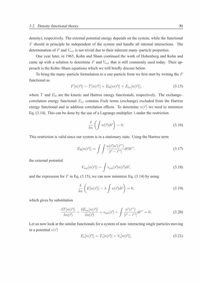
density), respectively. The external potential energy depends on the system, while the functionalF should in principle be independent of the system and handle all internal interactions. Thedetermination of F and Vext is not trivial due to their inherent many–particle properties.
One year later, in 1965, Kohn and Sham continued the work of Hohenberg and Kohn andcame up with a solution to determine F and Vext that is still commonly used today. Their ap-proach is the Kohn–Sham equations which we will briefly discuss below.
To bring the many–particle formulation to a one particle form we first start by writing the F
functional asF [n(�r)] = T [n(�r)] + EH[n(�r)] + Exc[n(�r)], (3.15)
where T and EH are the kinetic and Hartree energy functionals, respectively. The exchange–correlation energy functional Exc contains Fock terms (exchange) excluded from the Hartreeenergy functional and in addition correlation effects. To determine n(�r) we need to minimizeEq. (3.14). This can be done by the use of a Lagrange multiplier λ under the restriction
δ
δn
(∫n(�r)d�r
)= 0. (3.16)
This restriction is valid since our system is in a stationary state. Using the Hartree term
EH[n(�r)] =
∫ ∫n(�r)n′(�r ′)
|�r − �r ′| d�rd�r ′, (3.17)
the external potential
Vext[n(�r)] =
∫vext(�r)n(�r)d�r, (3.18)
and the expression for F in Eq. (3.15), we can now minimize Eq. (3.14) by using
δ
δn
(E[n(�r)] − λ
∫n(�r)d�r
)= 0, (3.19)
which gives by substitution
δT [n(�r)]
δn(�r)+
δExc[n(�r)]
δn(�r)+ vext(�r) +
∫n′(�r ′)
|�r − �r ′|d�r′ = 0. (3.20)
Let us now look at the similar functionals for a system of non–interacting single particles movingin a potential v(�r)
Es[n(�r)] = Ts[n(�r)] + Vs[n(�r)], (3.21)

32 Chapter 3. Density functional theory studies of thermoelectric materials
whereVs[n(�r)] =
∫v(�r)n(�r)d�r, (3.22)
and Ts is the kinetic energy functional. Minimizing Eq. (3.21) yields
δTs[n(�r)]
δn(�r)+ v(�r) = 0, (3.23)
for which the Schrodinger equation Hsφi = εiφi, with Hamiltonian Hs and eigenvalues εi is wellknown. The similarities between Eq. (3.20) and Eq. (3.23) are obvious if we take T = Ts suchthat
T [n(�r)] = −∫
φ†i (�r)∇2φi(�r)d�r (3.24)
andv(�r) = vext(�r) +
∫n(�r ′)
|�r − �r ′|d�r′ +
δExc[n(�r)]
δn(�r), (3.25)
and
n(�r) =N∑i
fi|φi(�r)|2, (3.26)
for N particles, where fi is the occupancy of the single particle orbital φi. Hence, to solveEq. (3.20) (that is to find the electron density n0(�r) that minimizes it), we only need to solve thesingle particle Schrodinger equation
(−1
2∇2 + v(�r)
)φi(�r) = εiφi(�r) (3.27)
The total energy E0 for the minimized electron density n0(�r) can now be found by expressingVext(�r) in terms of v(�r) through Eq. (3.18) and Eq. (3.25), such that
Vext[�r] = Vs[n0(�r)] − 2VH[n0(�r)] − δExc[n(�r)]
δn(�r). (3.28)
By substituting this back into Eq. (3.14), using Eq. (3.15) we get
E0 = Ts[n0(�r)] + Vs[n0(�r)] + VH[n0(�r)] − δExc[n0(�r)]
δn0(�r)− Exc[n0(�r)]. (3.29)
The first two terms are the energy functionals for the single particle Schrodinger equation, such
3.2. Density functional theory 33
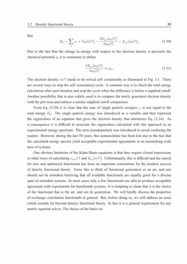
thatE0 =
∑i
εi + VH[n(�r)] − δExc[n0(�r)]
δn0(�r)− Exc[n0(�r)], (3.30)
Due to the fact that the change in energy with respect to the electron density is precisely thechemical potential μ, it is customary to define
δExc[n0(�r)]
δn0(�r)≡ μxc (3.31)
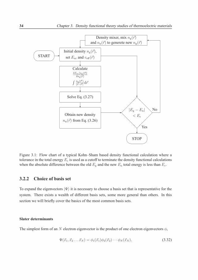
The electron density n(�r) needs to be solved self–consistently as illustrated in Fig. 3.1. Thereare several ways to stop the self–consistency cycle. A common way is to check the total energycalculation after each iteration and stop the cycle when the difference is below a supplied cutoff.Another possibility that is also widely used is to compare the newly generated electron densitywith the previous and enforce a similar supplied cutoff comparison.
From Eq. (3.30) it is clear that the sum of single particle energies εi is not equal to thetotal energy E0. The single particle energy was introduced as a variable and they representthe eigenvalues of an equation that gives the electron density that minimizes Eq. (3.14). Asa consequence it is difficult to associate the eigenvalues calculated with this approach to anexperimental energy spectrum. The term pseudoparticle was introduced to avoid confusing thereaders. However, during the last 50 years, this nomenclature has been lost due to the fact thatthe calculated energy spectra yield acceptable experimental agreements in an astonishing widearea of systems.
One obvious limitation of the Kohn-Sham equations is that they require closed expressionsor other ways of calculating vext(�r) and Exc[n(�r)]. Unfortunately, this is difficult and the searchfor new and optimized functionals has been an important cornerstone for the modern successof density functional theory. Some like to think of functional generation as an art, and oneshould not be mistaken believing that all available functionals are equally good for a diversespan of extended systems. In most cases only a few functionals are able to produce acceptableagreement with experiments for benchmark systems. It is tempting to claim that it is the choiceof the functional that is the art, and not its generation. We will briefly discuss the propertiesof exchange–correlation functionals in general. But, before doing so, we will address an issuewhich extends far beyond density functional theory. In fact it is a general requirement for anymatrix equation solver. The choice of the basis set.
34 Chapter 3. Density functional theory studies of thermoelectric materials
��
��START �
Initial density ng(�r),set Exc and veff(�r)
�
�CalculateδExc[ng(�r)]
δng(�r)∫ ng(�r′)
|�r−�r′|d�r
�
Solve Eq. (3.27)
�
Obtain new densitynn(�r) from Eq. (3.26)
���
��
�
��
��
�
��
��
�
��
��
�
|Eg − En|< Ec
No
Yes��
���STOP
�Density mixer, mix ng(�r)
and nn(�r) to generete new ng(�r)�
Figure 3.1: Flow chart of a typical Kohn–Sham based density functional calculation where atolerance in the total energy Ec is used as a cutoff to terminate the density functional calculationswhen the absolute difference between the old Eg and the new En total energy is less than Ec.
3.2.2 Choice of basis set
To expand the eigenvectors |Ψ〉 it is necessary to choose a basis set that is representative for thesystem. There exists a wealth of different basis sets, some more general than others. In thissection we will briefly cover the basics of the most common basis sets.
Slater determinants
The simplest form of an N electron eigenvector is the product of one electron eigenvectors φi
Ψ(�x1, �x2 . . . �xN) = φ1(�x1)φ2(�x2) · · ·φN(�xN), (3.32)

3.2. Density functional theory 35
usually referred to as a Hartree product. To obey the antisymmetry of the Pauli exclusion prin-ciple [6], the eigenvectors need to be expanded as Slater determinants of the one electron eigen-vectors. The simplest two particle Slater determinant is expanded as
Ψ(�x1, �x2) =1√2
(φ1(�x1)φ2(�x2) − φ1(�x2)φ2(�x1)) . (3.33)
Now, for the many–particle case, this gets far more complicated
Ψ(�x1, �x2 . . . �xN) =1√N !
∣∣∣∣∣∣∣∣∣∣
φ1(�x1) φ2(�x1) . . . φN(�x1)
φ1(�x2) φ2(�x2) . . . φN(�x2)...
... . . . ...φ1(�xN) φ2(�xN) . . . φN(�xN)
∣∣∣∣∣∣∣∣∣∣. (3.34)
Such many–particle Slater determinants are very demanding to calculate and only a single Slaterdeterminant is usually implemented in Kohn-Sham DFT (and Hartree–Fock) procedures. Butit is important to emphasize that there exist generalized Kohn-Sham schemes that include acombination of several Slater determinants to calculate exchange kernels and correlation effectson a perturbative level. More accurate many–particle Configuration Interaction (CI) or Multi–Configurational Self–Consistent Field (MCSCF) calculations also require a multi–term Slaterdeterminant. For simple molecules it is feasible to use the full Slater approach, but for extendedsystems this is not an option due to the unfavourable scaling of the calculation of the determinant.To use the Slater approach or not, knowledge about the single particle eigenvectors φi is neces-sary. The most basic type of eigenvectors are hydrogen like orbitals, e.g. Slater–Type Orbitals(STO) [7].
Linear combination of atomic orbitals
Linear combination of atomic orbitals (LCAO) is based on single atomic orbitals (e.g. STOs). Toset up the basis, the atomic orbitals are expanded up to a given cutoff. To increase flexibility andspeed Gaussian–Type Orbitals (GTO) [8] are often used instead of STOs. A single GTO does notreproduce a hydrogen like orbital, but the operator integrals are faster to calculate (they have anexplicit form). The atomic orbitals can be efficiently calculated and are still extensively used inmolecular calculations. Such basis sets are however prune to failure if the states are delocalizedwith respect to the atom sites and are thus not optimal for many materials.

36 Chapter 3. Density functional theory studies of thermoelectric materials
Pseudo–potentials
For calculations beyond simple molecules additional approximations of the basis set are neces-sary to improve performance. One of the first and simplest approaches was the use of pseudo–potentials. The main idea is to separate the core and valence electrons and exclude the core statesfrom the self–consistent calculation. The core states are predetermined for all atoms, based onatomic calculations. The contributions from the core states are included in the Kohn-Sham equa-tions through the external potential. The pseudo–potential approach simplifies the choice ofbasis set due to the exclusion of a great number of electrons. However, a proper basis set is stillneeded for the valence electrons and at the same time this basis set should be compatible withthe pseudo–potentials such that there is acceptable overlap.
Plane wave based basis functions
Plane wave basis sets exploit the periodicity of structures [9] (Chap. 2 and App. F). Basicallyplane waves are waves expanded based on the Brillouin zone reciprocal vectors. The plane wavesneed a large amount of coefficients to describe a localized state, but combined with the pseudo–potential approach they are very efficient and have some advantages over the orbital basis sets(mainly non–local expansions). Plane wave basis sets yield a simple form of the Kohn-Shamequations and are thus easy to implement. Due to the generality of the plane waves the samebasis set can be utilized for all atom species.
Linearized Augmented plane waves (LAPW) [10] (Sec. 4.2) incorporate atomic–like states inthe atomic region, while envelope functions are used to expand the interstitial (or bonding) states.The envelope functions are determined by plane wave expansions. Similarly, Linear Muffin–Tin–Orbitals (LMTO) [11] are obtained if the envelope functions are expanded by Hankel functions(solutions of the Laplace equation). The main difference between LAPW and LMTO lies in theinterstitial region, where the energy dependence is excluded in the LMTO approach. This makesLMTO more feasible for closed packed structures.
A generalization of the LAPW and pseudo–potential method is called the Projected Aug-mented Wave (PAW) [12] method. It is more efficient while retaining the accuracy of the LAPWapproach. As a consequence it is praised as one of the best basis sets for first–principle calcula-tions [13, 14] of materials.

3.2. Density functional theory 37
3.2.3 Exchange–correlation functionals
Before addressing the exchange–correlation functionals we will briefly consider an importantaspect known as the derivative discontinuity of the exchange–correlation functionals. Unfortu-nately we will see that this is an inherent feature of the Kohn-Sham equations. This sectionclosely follows the work published by Perdew et al. [15, 16].
Let us start with a system containing N = N ′ + ω electrons, where N ′ is a positive integerand 0 ≤ ω ≤ 1. The introduction of fractional electron numbers is unphysical, but a timeaveraged mixing of N ′ and N ′ + 1 is possible [16]. The parameter ω controls the mixing of theΨN ′ and ΨN ′+1 states such that
N = N ′ + ω, (3.35)
= (1 − ω)N ′ + ω(N ′ + 1), (3.36)
sinceN =
∫nN(�r)d�r, (3.37)
nN(�r) = (1 − ω)nN ′(�r) + ωnN ′+1(�r). (3.38)
From Eq. (3.30) we know that E0 is a functional of n(�r). Hence E0 can be written as
E0[nN(�r)] = (1 − ω)E0[nN ′(�r)] + ωE0[nN ′+1(�r)], (3.39)
which are continuous lines as a function of N ′ [16, 17]. Thus, ∂E0/∂N should be ill–defined foreach integer number of particles in the system.
The ionization potential I for an atom X with N electrons is defined as the process
X → X+ + e−, (3.40)
withI(N) = E0(N − 1) − E0(N), (3.41)
where the outermost and weakest bonded electron is removed to infinity, such that there is nointeraction between the ion and the electron. Similarly the electron affinity A is defined as
X− → X + e−, (3.42)
38 Chapter 3. Density functional theory studies of thermoelectric materials
withA(N) = E0(N) − E0(N + 1). (3.43)
We can relate I and A to a change in n(�r) such that
I(N) = − δE0
δnN(�r)
∣∣∣∣N ′−1
, (3.44)
andA(N) = − δE0
δnN(�r)
∣∣∣∣N ′+1
. (3.45)
Looking back at Eq. (3.29) we see that the density functional derivative of the external potentialVs and electrostatic potential VH is inherently continuous, which leaves the kinetic energy Ts andexchange–correlation energy Exc to obey the fundamental discontinuity property. The kineticenergy derivative and its discontinuity is trivial due to the direct evaluation of the pseudo particleorbitals. Hence, it is the exchange–correlation functional that ought to reproduce the discontinu-ities. The difference between the ionization potential and electron affinity is usually defined asI − A, which, if the system is charge neutral, determines the fundamental band gap Eg,
Eg(N) = I(N) − A(N), (3.46)
=δT
δn(�r)
∣∣∣∣N+1
− δT
δn(�r)
∣∣∣∣N−1
+δExc
δn(�r)
∣∣∣∣N+1
− δExc
δn(�r)
∣∣∣∣N−1
, (3.47)
= ΔKS + Δxc, (3.48)
where ΔKS and Δxc are the kinetic and exchange–correlation derivative differences, respectively.For all systems, except the simplest non–interacting ones, Δxc = 0 [15]. This is a paradox,since, by construction, Exc should be continuously differentiable and independent of the energy.Unfortunately there is no easy way to escape this problem, except going past the Kohn-Shamscheme to a more generalized Kohn-Sham scheme (gKS) that incorporates energy dependentfunctionals based on e.g. Fock terms (through the orbital dependence). We will now present twocommon ways of expanding the exchange–correlation functionals and introduce a relatively newhybrid approach including exact exchange (Fock) terms in the gKS formalism. The subsequentfunctionals all have spin–polarized versions, but to simplify notation they are not discussed.These and other failures of modern implementations of density functional theory are frequentlydiscussed in the literature [18, 19, 20] and readers interested in the subject should consult thereferred papers.

3.2. Density functional theory 39
Local density approximation
One of the first approximations of the exchange–correlation energy was based on the local densityapproximation (LDA) [4, 5]
ELDAxc =
∫εhomxc (n(�r))d�r, (3.49)
where εhomxc (n(�r)) = εhom
x (n(�r)) + εhomc (n(�r)) is the energy from the homogeneous free electron
gas. The exchange contribution εhomx (n(�r)) is known exactly as
εhomx (n(�r)) = −3e2
4
(3
π
)1/3
n(�r)4/3, (3.50)
where e is the electron charge. See Ref. [21] (contribution by V. Sahni, page 217). The correla-tion contribution εhom
c (n(�r)) however, has to be parametrized. Most implementations today usea parameterization based on Quantum Monte Carlo (QMC) simulations done by Ceperley andAlder [22]. At first it came as a surprise that LDA gave reasonable agreement with experiments,even for systems well beyond the free electron gas. It was later discovered that this was due to er-ror cancellation in the evaluation of the over–compensated exchange and the under–compensatedcorrelation [23, 24] functionals.
Generalized gradient approximation
There is no doubt that the local form of the local density approximation will produce inaccu-rate results for systems deviating from the free electron gas regime. Therefore a more generalapproach was introduced, called the generalized gradient approximation (GGA) [25],
EGGAxc (n(�r)) =
∫f(n(�r),∇n(�r))d�r, (3.51)
where f(n(�r),∇n(�r)) is a general functional of the density and its gradient. The differencebetween semi–local GGA functionals depends on the choice of f(n(�r),∇n(�r)) and they canthus differ substantially from each other. A discussion of the wide range of GGA functionals isnot the intention of this thesis, so readers are referred to the literature and Ref. [26] for a quickoverview (primarily Sec. 1.6). However, it should be emphasized that the GGA approach is stilllocal, but corrected by the gradient ∇n(�r) such that it is ultimately semi–local.

40 Chapter 3. Density functional theory studies of thermoelectric materials
Hybrid LDA/GGA
One major concern with the general LDA and GGA functionals used today is the lack of delo-calization correction [19], which tends to spread the electron charge. This correction is inherentto the exact exchange (Fock terms) [27] and is excluded for the aforementioned approaches dueto the implicit energy (through the orbitals) dependence, and thus the performance penalties thatfollow.
Most hybrid functionals include a quarter portion of exact exchange and evaluate the remain-der exchange from the base functional. The concept of the quarter mixing ratio is based on workdone by Ernzerhof and coworkers [28, 29, 30]. One of the most common hybrid functionals usethe PBE functional as a base and is therefore called PBE0 [31]. It is defined as
EPBE0 =1
4EHF
x +3
4EPBE
x + EPBEc , (3.52)
where the subscripts (x) and (c) term the exchange and correlation parts, respectively. The super-script signalizes how to evaluate the given energy, where HF is the Hartree energy and the exactexchange (this is thus the well known Hartree–Fock [27] contribution). The PBE superscript tellsus that the exchange and correlation should be evaluated from the PBE functionals. Similarlyone can define range separated hybrid functionals, like the HSEx [32], defined as
EHSEx =1
4EHF,sr
x +3
4EPBE,sr
x + EPBE,lrx + EPBE
c , (3.53)
where (sr) and (lr) describe the short and long range parts of the exchange energy. This rangeseparation is defined by separating the Coulomb kernel such that
1
r=
erfc(μr)
r+
erf(μr)
r, (3.54)
where μ determines the range separation. For the HSE03 [32] functional this is defined as μ =
0.3 A−1. The range separation is motivated for two reasons: first, it allows the calculation ofthe exact exchange on a coarser grid, thus improving convergence [33]; second, one has thepossibility to investigate the range extension of the exact exchange energy. Recent reviews ofthe hybrid functionals reveal a very good compromise between accuracy and performance fora wide range of benchmark systems [33, 34, 35]. Although, depending on implementation, anorder of magnitude increase in computational time has to be expected over the traditional LDAand GGA functionals. Memory requirements also increase due to the calculation and storage ofthe orbitals. There are still some questions as to whether the quarter portion of exact exchange

3.3. Electronic structure and bonding 41
can be used for all systems (metallic systems in particular do not show much improvement [33])or if there should be a headroom for tuning this portion. Future studies will reveal the necessaryanswers to these questions.
3.3 Electronic structure and bonding
To analyze the electronic structure and bonding of materials it is common to consider the densityof states and band structure. They reveal hybridization, chemical shifts and bonding proper-ties indirectly. We like to term such analysis state–resolved. Quantitative experimental veri-fications can be done by X–ray photoemission spectroscopy (XPS), ultra–violet photoemissionspectroscopy (UPS), a diverse selection of band gap measurements and electron energy loss spec-troscopy (EELS). However, these techniques usually contain a wealth of effects not present inthe calculation of the ground state density of states (e.g. excitations, resonances and secondaryeffects). Thus, a direct verification of the validity of the calculation can sometimes be difficult.
However, and especially so for density functional calculations, all properties are calculatedfrom the electron density. This density is thus also available for direct analysis and contraryto the state–resolved analysis one can perform spatial–resolved analysis of electron transfer inthe system. These transfers are associated with the electron rearrangement to set up the bondsbetween the ions in the system. Experimental verifications can be done directly by obtaining thestructure factors from X–ray and electron diffraction. These structure factors can be transformedto the real space by a Fourier transformation [36] (Sec. 6.5) and are then directly comparable tothe electron density. Although such approach is uncommon today, we believe such analysis willbe more important in the future.
3.3.1 Electron density analysis
Electron transfer
The electron density contains all necessary information to compute observables within DFT.Since the bonds are inherently determined by electron transfer it also serves as a perfect base forbond analysis and an alternative or complement to the state–resolved density of states analysisthat is common practice these days [37] (Chap. 5). The electron transfer ρb can be determinedby
ρb(�r) = ρc(�r) − ρr(�r), (3.55)
42 Chapter 3. Density functional theory studies of thermoelectric materials
where ρc and ρr are the crystal and reference electron density, respectively. The crystal electrondensity is obtained directly from calculations, but ρr still needs to be determined.
From a theoretical point of view we can use the procrystal [38] electron density ρp as areference ρr. Generated from a superposition of free atomic electron densities embedded in thecrystal unit cell, this reference should be free of bonding features.
Different experimental methods exist to determine the electron density and/or electron trans-fer. One approach is to compare spectroscopic data with an elemental reference ρm [39, 40, 41,42], and the relative intensity difference can be converted to occupancy numbers [43]. However,this approach is burdened by differences in the reference bonds and could yield unreliable resultsif two elements with different bonding characteristics are used.
A more direct approach is to perform diffraction experiments and refine the structure factorsby starting from overlapping atomic orbitals [38, 44, 45]. This reference is in principle equivalentto the previously discussed procrystal. The structure–factor refinement is stopped when sufficientagreement with experimental diffraction intensities is reached.
The procrystal represents a consistent reference in electron transfer analysis, but may to-day be difficult to use as a reference experimentally due to the lack of established and efficientexperimental procedures to obtain a large number of structure factors.
3.3.2 A few examples
To demonstrate the spatially resolved electron transfer bond analysis and its strengths, we heregive three standard examples; the covalently bonded silicon, the ionic sodium chloride and themetallic aluminium. In addition we give a more complicated example of the filled phospho-rus skutterudite LaFe4P12. All calculations were done on a dense augmented grid where theall–electron density was regenerated [13] to get rid of the problematic compensator charges in-herent to most of the density functional implementations using plane waves. In all examples therespective procrystal has been used as the electron density reference.
Covalent silicon
Elemental silicon, Si, was chosen as it is well known from the literature to contain exclusivelycovalent bonds. It is also relatively simple due to the high symmetry and small primitive cell. InFig. 3.2 we show the electron accumulation and depletion arising from the positive and negativeρb, respectively. The electron accumulation in Fig. 3.2(a) clearly illustrates the covalent characterof silicon. The covalent bonds are set up by rearranging the electron density around Si, moving

3.3. Electronic structure and bonding 43
(a) Electron accumulation (b) Electron depletion
Figure 3.2: (a) Electron accumulation (positive ρb) and (b) depletion using the respective pro-crystal as a reference for Si. Isosurfaces are drawn at 0.008/bohr3.
electron density from non–directional to the directional Si–Si parts of the crystal (see Fig. 3.2(b)).
(a) Electron accumulation (b) Electron depletion
Figure 3.3: (a) Electron accumulation (positive ρb) and (b) depletion using the respective pro-crystal as a reference for NaCl. Na in gray and Cl in black. Isosurfaces are drawn at 0.005/bohr3.
Ionic sodium chloride
Elemental sodium–chloride, NaCl, serves as a prototype example of ionic bonding and is usuallyused as a textbook example, making the structure and bonding properties well known. Similarto silicon we illustrate the electron accumulation and depletion in Fig. 3.3. From this figure, theionic character, with local depletion (Na+) on the Na and local accumulation (Cl−) on the Cl

44 Chapter 3. Density functional theory studies of thermoelectric materials
sites are reproduced.
Metallic aluminium
To represent metallic bonding, elemental aluminium, Al, was chosen. Similarly to Si and NaClits structure and bonding properties are well known from the literature and from Fig. 3.4 we seethat the metallic character is reproduced. Electron density is depleted close to the Al site andredistributed between the Al sites in a non–directional manner.
(a) Electron accumulation (b) Electron depletion
Figure 3.4: (a) Electron accumulation (positive ρb) and (b) depletion using the respective pro-crystal as a reference for Al. Isosurfaces are drawn at 0.004/bohr3.
Phosphorus filled skutterudite LaFe4P12
As a final example we include the lanthanum filled iron phosphorus skutterudite LaFe4P12 (seePaper I for structure information). The reason for this is that electron transfer analysis of thiscompound reveals what seems to be a unique electron arrangement around the lanthanum ions.This could explain why the filled skutterudite structure so successfully reduces the thermal con-ductivity. In addition, the skutterudite structure contains covalent bonds. In Fig. 3.5 the electronaccumulation and depletion are given for the FeP6 octahedral arrangement. The biased (towardsP) covalent bond between Fe and P can be explained from the difference in electronegativity.Similarly in Fig. 3.6, the electron transfers between the P ions in the P4 ring are covalent and dueto the rectangular shape, one bond is stronger, which is nicely reproduced by this analysis.
Finally in Fig. 3.7 the electron transfer around the La ion is shown. The electron accumu-lations (only partially shown due to the cutout of the unit cell) responsible for the La–P bondscan be seen on the border in the La plane. Close to the La ion, elongated electron accumulationis aligned towards the P ions. These electron accumulations could set up restrictions of the Lamotion during vibrational perturbations and thus contribute to the significant reduction in thelattice thermal conductivity [46, 47].

3.3. Electronic structure and bonding 45
(a) Electron accumulation (b) Electron depletion
Figure 3.5: (a) Electron accumulation (positive ρb) and (b) depletion between the grey Fe andgreen P in the octahedra using the respective procrystal as a reference. Isosurfaces are drawn at0.024/bohr3.
(a) Electron accumulation (b) Electron depletion
Figure 3.6: (a) Electron accumulation (positive ρb) and (b) depletion between the green P ionsusing the respective procrystal as a reference. Isosurfaces are drawn at 0.017/bohr3.

46 Chapter 3. Density functional theory studies of thermoelectric materials
(a) Electron accumulation (b) Electron depletion
Figure 3.7: (a) Electron accumulation (positive ρb) and (b) depletion around the black La usingthe respective procrystal as a reference. The Fe ions are shown in grey. Isosurfaces are drawn at0.0025/bohr3.

3.4. Transport properties 47
3.4 Transport properties
The performance of thermoelectric materials is determined by the figure–of–merit zT as pre-viously discussed. To determine zT extensive knowledge about the system is required. Morespecifically we need to determine the electrical and thermal conductivity, and the Seebeck coef-ficient, all preferably at different temperatures. Calculations of these properties are not trivial,due to several intricate problems with the first–principle calculations that serve as a baselinefor the transport calculations. It should also be mentioned that the experimental determinationof these properties is difficult. In this chapter we will introduce a semi–classical procedure tocalculate the electrical conductivity σ and the Seebeck coefficient α, which together determinethe power factor α2σ. In addition we calculate the electrical thermal conductivity such that thefigure–of–merit can be determined for a given lattice thermal conductivity.
We now develop a general approach by discussing the strengths, pitfalls and implementationof the semi–classical Boltzmann transport equations. Most of the derivation of the distributionfunction and the Boltzmann transport equation is based on the textbook of Ashcroft and Mer-min [9] (Chap. 12, 13 and 16). Before the explicit Boltzmann equation is derived, we brieflydiscuss electron transport in solids in general. We then dedicate a section of prediction based onsimple band engineering and propose band structure characteristics that give the largest powerfactor and figure–of–merit. Readers of this section should be aware that where applicable theposition and wave vector are dependent on time. The time dependence is shown explicitly whereneeded. However, for some variables with an implicit time dependence through the position andwave vector (e.g. equilibrium distribution function), explicit time dependence is still shown. Thisnotation is not strictly valid, but has been chosen for simplicity.
3.4.1 Electronic transport in solids
According to Bloch theory [9] (Chap. 12), electrons do not scatter if the lattice is periodic andperfect. Such lattices do not exist in reality and scattering events are usually classified in threemain categories;
• Scattering from thermal vibrations in the lattice. Due to vibrations in the lattice eachion will deviate from the equilibrium position and generate imperfections in the crystal.Electrons scatter locally from these imperfections. One further separates these vibrationsinto acoustical and optical vibrations, based on the vibrational character. Lattice vibrationsprimarily arise due to thermal energy and are thus strongly temperature dependent.

48 Chapter 3. Density functional theory studies of thermoelectric materials
• Scattering from deviations from the atom positions in the perfect crystal (e.g. impuritiesand vacancies) and/or periodic lattice (e.g. boundary effects). Usually the two are relatedand imperfections can in general be local or extended, depending on type.
• Scattering based on strong electron–electron interactions. These types of scattering eventsarise due to exact exchange (Hartree–Fock) and screening interactions. Typical relaxationtimes (the time between each collision) for these scattering events are about 102-106 [9](Chap. 17) times larger than vibrational scattering and scattering from imperfections andcan in most cases be safely discarded. We would have to go to very low temperature toremove any thermal vibration for electron–electron scattering to be an observable effect insamples free of imperfections.
The electronic transport depends on the distribution of electrons. This distribution generallydiffers from the equilibrium Fermi distribution and we will term its function g in the following.The distribution function will depend on both the position vector �r, the wave vector �k and time t.We will however suppress the �r dependence until we discuss the Boltzmann equation in the nextsection. Before exploring this distribution function, let us first discuss the scattering process.We will disregard spin effects in the derivation, but emphasize that most of these equations areequally valid for bosons and fermions. Let us define a scattering probability Γ�k,�k′,n,n′ , where �k
and �k′ are the initial and final wave vectors, and similar for the band index n. The scattering ratecan now be defined as
1
τ outn (�k, t)
=
∫d�k′dn′
Ω
(1 − gn′(�k′, t)
)Γ�k,�k′,n,n′ , (3.56)
where Γ�k,�k′,n,n′d�k′/Ω is the probability per unit time that a scattering event from �k and n to d�k′dn′
within�k′ and n′ takes place. The unoccupied distribution function 1−gn′(�k′, t) is needed since theoccupied (and thus no scattering) states are determined by gn′(�k′, t). By integrating all possible�k′, n′ and normalizing using the �k-space volume Ω (taken to be (2π)3 or 4π3, depending onwhether to account for spin degeneracy) the total rate is obtained. Notice that the relaxation timeτn(�k) is not explicitly a function of �k (although we still persist on this notation for simplicity),but depends on �k through Γ�k,�k′,n,n′ and gn′(�k′, t).
The change in gn(�k, t) for an infinitesimal time interval dt is the probability for scatteringout of �k times the distribution function gn(�k, t), that is
(dgn(�k, t)
dt
)out
= −gn(�k, t)
τ outn (�k)
. (3.57)
3.4. Transport properties 49
The out scattering reduces the states in �k, hence the minus.In Eq. (3.56) and Eq. (3.57) scattering out of �k was defined. However, we simultaneously
need to account for the inbound scattering processes. To obtain this we use Eq. (3.56) andsubstitute 1 − gn′(�k′, t) by gn′(�k′, t) and Γ�k,�k′,n,n′ by Γ�k′,�k,n′,n (now termed 1/τ in
n (�k, t)). To getthe inbound scattering change in gn(�k, t) we multiply this by the unoccupied distribution function1 − gn(�k, t), such that (
dgn(�k, t)
dt
)in
=1 − gn(�k, t)
τ inn (�k)
. (3.58)
Adding the outbound and inbound terms yields the total change in gn(�k) as
(dgn(�k, t)
dt
)total
=
(dgn(�k, t)
dt
)out
+
(dgn(�k, t)
dt
)in
, (3.59)
= −gn(�k, t)
∫d�k′dn′
Ω
(1 − gn′(�k′, t)
)Γ�k,�k′,n,n′
+(1 − gn(�k, t)
) ∫d�k′dn′
Ω
(gn′(�k′, t)
)Γ�k′,�k,n′,n. (3.60)
The scattering probability Γ can in general be very complex. For simple impurity scatteringone can for example develop an expression for Γ based on the “Golden rule” of Fermi. See forexample Ref. [48] (Sec. 3.2) and [1] (Sec. 8.3). For vibrational scattering an entirely differentprocess needs to be developed to also include the electron–phonon interaction. It should be clearto the reader that the general scattering problem is comprehensive. Even many–body problemsfree of scattering are problematic to solve and it should not come as a surprise that we need tointroduce approximations.
We will now assume that a scattering event is not determined by the initial distribution func-tion gn(�k), and that the scattering events maintain the thermodynamic equilibrium. Furthermore,we assume that the relaxation time τn(�k, t) is only dependent on the band index n and the wavevector �k. Hence, no implicit dependence through gn(�k, t) or Γ is allowed. Now, the in scatter-ing is g0
n(�k, t) times the probability dt/τn(�k) of a scattering event in the time interval dt. Morespecifically (
dgn(�k, t)
dt
)total
RTA
=g0
n(�k, t) − gn(�k, t)
τn(�k, t), (3.61)
where g0n(�k) is the equilibrium distribution function. All approximations that led to Eq. (3.61)
and hence the equation itself are usually called the relaxation time approximation (RTA). This
50 Chapter 3. Density functional theory studies of thermoelectric materials
approximation is very common and used in almost all transport calculations today. The in andout scattering terms can be identified as
(dgn(�k, t)
dt
)in
RTA
=g0
n(�k, t)
τn(�k, t), (3.62)
(dgn(�k, t)
dt
)out
RTA
= −gn(�k, t)
τn(�k, t). (3.63)
We will see later, that further approximations need to be introduced to make the transport calcu-lations tractable for extended systems.
3.4.2 The Boltzmann equation
In this section the Boltzmann equation is derived from the semi–classical equations of motion [9](Chap. 12) by considering a change in gn(�r,�k, t). The change of a position vector is known as
d�r
dt= �v(�r,�k, t), (3.64)
where �v(�r,�k, t) is the quantum mechanical velocity average of the velocity operator. Similarly,the change in wave vector from external forces is
d�k
dt=
1
h�F (�r,�k, t) (3.65)
= − e
h
(�E(�r,�k, t) − 1
c�v(�r,�k, t) × �H(�r,�k, t)
), (3.66)
where �F (�r,�k, t) is the external field that contains both the electric �E(�r,�k, t) and magnetic�H(�r,�k, t) fields, while c is the speed of light. A change of gn(�r,�k, t) in the time interval dt
can now be determined by the modified equations of motion, such that
gn(�r,�k, t)d�rd�k = gn
(�r − �v(�r,�k, t)dt,�k −
�F (�r,�k, t)
hdt, t − dt
)
× d�r(t − dt)d�k(t − dt). (3.67)
Through Liouville’s theorem [9] (Chap. 12) the �r�k phase space is conserved during a dt change.Thus, the infinitesimal terms on both sides can be cancelled. It should be clear that Eq. (3.67)

3.4. Transport properties 51
does not account for scattering events. These terms need to be added and we get
gn(�r,�k, t)
dt=
gn
(�r − �v(�r,�k, t)dt,�k − �F (�r,�k,t)
hdt, t − dt
)dt
+
(dgn(�r,�k, t)
dt
)total
. (3.68)
Expanding to linear order in dt and taking the limit dt → 0 reveals the famous Boltzmannequation
dgn(�r,�k, t)
dt+ �v(�r,�k, t) · ∂gn(�r,�k, t)
∂�r+
1
h
∂gn(�r,�k)
∂�k· �F (�r,�k, t) =
(dgn(�r,�k, t)
dt
)total
. (3.69)
The expressions on the left hand side control the total change in gn(�r,�k, t), the change fromdiffusion and the change from applied fields, respectively. On the right hand side we have thescattering contributions.
3.4.3 Non–equilibrium distribution function
We need knowledge about the non–equilibrium distribution function to be able to utilize theBoltzmann equation and will now go through derivations that lead it to a tractable form. Thederivations follow closely the textbook of Ashcroft and Mermin [9] (Chap. 12, 13 and 16).
Assume that the infinitesimal phase space d�rd�k contains dN electrons such that
dN = gn(�r,�k, t)d�rd�k
4π3. (3.70)
The distribution function gn(�r,�k, t) can now be determined from the time relaxation approxima-tion if we assume that all previous scattering in the volume d�r ′d�k′ from t′ are scattered into thevolume d�rd�k at t. This is a reasonable assumption as the particles will follow the semi–classicalequations of motion from t′ to t. From Liouville’s theorem [9] (Chap. 12), d�r ′d�k′ = d�rd�k. Thein scattered part of the relaxation time approximation (Eq. (3.62)) can be integrated over t′ ininfinitesimal dt′ parts from −∞ to t, such that the distribution function now becomes
∫ t
−∞
g0n(�r,�k, t′)
τn(�r,�k, t′)dt′, (3.71)

52 Chapter 3. Density functional theory studies of thermoelectric materials
which need to be modified, since there can be scattering events between t′ and t. We need theprobability Pn(�r,�k, t, t′) of no further scattering after t′, but before t, to be multiplied into theintegrand. Hence,
gn(�r,�k, t) =
∫ t
−∞
g0n(�r,�k, t′)Pn(�r,�k, t, t′)
τn(�r,�k, t′)dt′. (3.72)
Substituting this back into Eq. (3.70) yields
dN =d�rd�k
4π3
∫ t
−∞
g0n(�r,�k, t′)Pn(�r,�k, t, t′)
τn(�r,�k, t′)dt′. (3.73)
We now need to determine the probability Pn(�r,�k, t, t′). This can be done by noting that
Pn(�r,�k, t, t′) = Pn(�r,�k, t, t′ + dt′)
(1 − dt′
τn(�r,�k, t′)
), (3.74)
since the number of particles that undergo no scattering between t′ and t is less than betweent′ + dt′ and t by the ratio 1 − dt′/τn(�r,�k, t′). Taking the limit dt′ → 0 we get a differentialequation
∂Pn(�r,�k, t, t′)
∂t′=
Pn(�r,�k, t, t′)
τn(�r,�k, t′), (3.75)
with solution
Pn(�r,�k, t, t′) = exp
(−
∫ t
t′
dt′′
τn(�r,�k, t′′)
), (3.76)
subject to the boundary condition Pn(�r,�k, t, t) = 1. We can now substitute Eq. (3.75) intoEq. (3.72) and obtain
gn(�r,�k, t) =
∫ t
−∞
g0n(�r,�k, t′)
(∂
∂t′Pn(�r,�k, t, t′)
)dt′. (3.77)
Integrating by parts yields
gn(�r,�k, t) = g0n(�r,�k, t) −
∫ t
−∞
Pn(�r,�k, t, t′)
(d
dt′g0
n(�r,�k, t′)
)dt′, (3.78)
if we also set the condition Pn(�r,�k, 0,−∞) = 0, that is, that no particles can reach t without ex-periencing scattering events. Next, is the time derivative of the equilibrium distribution function.

3.4. Transport properties 53
Expanding the derivative as
dg0n(�r,�k, t′)
dt′=
∂g0n(�r,�k, t′)
∂εn(�k, t′)
∂εn(�k, t′)
∂�k· d�k
dt′+
∂g0n(�r,�k, t′)
∂T (�r, t′)
∂T (�r, t′)
∂�r· d�r
dt′
+∂g0
n(�r,�k, t′)
∂μ(�r, t′)
∂μ(�r, t′)
∂�r· d�r
dt′, (3.79)
and applying the semi–classical equations of motion from Eq. (3.64) and Eq. (3.66) yields,
gn(�r,�k, t) = g0n(�r,�k, t) (3.80)
−∫ t
−∞
Pn(�r,�k, t, t′)
[∂g0
n(�r,�k, t′)
∂εn(�k, t′)�vn(�k, t′)
×(−e �E(�r,�k, t) −∇μ(�r, t′) −
(εn(�k, t′) − μ(�r, t′)
T (�r, t′)
)∇T (�r, t′)
)]dt′.
This is a very general function. At first sight it might seem that Eq. (3.80) is independent of amagnetic field. This is not the case as it enters implicitly by modifying �r and �k. We can induceadditional approximations to simplify Eq. (3.80) further. If we assume a spatial uniform electricfield and temperature gradient, the �r dependence drops out of �E and ∇T . The same assumptioncan also be made for the relaxation time and the chemical potential (depends on space throughT ) such that the �r dependence drops out of the integrand. The equilibrium distribution functiong0
n(�r,�k, t) is dependent on �r through T and on �k through εn(�k, t) and is also under the previousassumptions independent on �r. In this thesis, we will only work with electrons, so we nowabbreviate
g0n(�r,�k, t) = f(�k, t), (3.81)
where f(�k, t) is the equilibrium Fermi distribution function.Even though we developed an expression for gn(�r,�k, t), we have yet to give a more specific
form of Pn(�r,�k, t, t′), except for the one in Eq. (3.76). If we now assume a relaxation time thatdepends on energy only, the probability becomes trivial from Eq. (3.76), such that
Pn(�k, t, t′) = e−(t−t′)/τn(�k), (3.82)
where the �k dependence in τn(�k) enters implicitly through εn(�k, t). By applying all these ap-

54 Chapter 3. Density functional theory studies of thermoelectric materials
proximation to Eq. (3.80), we obtain
gn(�k, t) = g0n(�k, t) (3.83)
−∫ t
−∞
e−(t−t′)/τn(�k)
[∂f(�k, t′)
∂εn(�k, t′)�vn(�k, t′)
×(−e �E(t′) −∇μ(t′) −
(εn(�k, t′) − μ(t′)
T (t′)
)∇T (t′)
)]dt′.
Still, the time integral of Eq. (3.83) is non–trivial. Based on an expansion of Eq. (3.66) we canapproximate a change in wave vector �k(t) from modifications due to �E(t) as
�k(t) ≈ �k(0) − e �E(t)t
h. (3.84)
The main contribution to the integrand in Eq. (3.83) appears at t ≈ τ . Based on the fact thatτ ∝ 10 fs [9] (Chap. 1) the modifications to �k(0) is thus rather small. Similarly one can argue thatperturbation of the temperature within the same time slit is small. Hence, the time integral canbe taken at a constant electric field and temperature gradient. Unfortunately, it is not possible togenerate a linear approximation for the perturbation of magnetic fields. However, in the absenceof magnetic field, the time dependence of �k disappears and the time integral is trivial, such that
∫ t
−∞
e−(t−t′)/τn(�k)dt′ = τn(�k), (3.85)
since t always is positive. The combination of Eq. (3.83) and Eq. (3.85) under the given approxi-mations serve as a base to obtain tractable equations for the transport coefficients. It is importantto emphasize that Eq. (3.83) satisfy the Boltzmann equation in Eq. (3.69) and is this a validsolution of the electron transport.
3.4.4 The Boltzmann transport equations
Based on the above derivation of the Boltzmann equation and distribution function we will nowdevelop the specific Boltzmann transport equations. The electrical current density can be definedas
�J = nq�v, (3.86)
where n is the number of charge carriers per volume unit, q is the elementary charge and �v isthe carrier drift velocity. Now, n is determined by the distribution function integrated, while for

3.4. Transport properties 55
electrons, q = −e. Since multiple bands can contribute, we need to sum each band index n. Thisgives
�J = − e
Ω
∑n
∫gn(�k)�vn(�k)d�k, (3.87)
where Ω is the volume of the �k–space. At this time it is important to notify the reader; one shouldnot be easy minded and believe that Eq. (3.87) is of a general form (e.g. only �k dependence inthe integrand). A significant number of approximations was introduced to reduce the dimensionof the distribution function. Generally, it will also depend on �r and t. The electrical current canalso be expressed as
�J = σ �E − χ∇T, (3.88)
and similarly for the thermal current
�JQ = Tχ�E − κ0∇T, (3.89)
where σ is known as the electrical conductivity, χ and κ0 are thermal constants in front of thethermal gradients for the electrical and thermal current, respectively. As usual �E is the appliedelectric field and T is the temperature. In general σ, χ and κ0 are tensors. The Seebeck coefficientα is defined as the ratio between the applied electrical field and the temperature gradient at zeroelectrical current. More specifically
α =�E
∇T, (3.90)
which for zero current givesα = σ−1χ, (3.91)
from Eq. (3.88). We will now derive expressions for σ and χ. Let us continue to use the sim-plified distribution function gn(�k, t) developed in the last section. By substituting Eq. (3.83)into Eq. (3.87) using Eq. (3.85) and assuming constant (in time) electrical field and temperaturegradient we get
�J =e
Ω
∑n
∫τn(�k)
(−∂fn(�k)
∂ε(�k)
)�vn(�k)
(�vn(�k) ·
[e �E + ∇μ +
ε(�k) − μ
T∇T
])d�k. (3.92)
Comparing Eq. (3.88) and Eq. (3.92) reveal that the electrical conductivity can be written as
σ =e2
Ω
∑n
∫τn(�k)
(−∂fn(�k)
∂ε(�k)
)�vn(�k)�vn(�k)d�k. (3.93)

56 Chapter 3. Density functional theory studies of thermoelectric materials
We determine χ in the same way, looking at the component in front of the temperature gradientin Eq. (3.92). This gives
χ =e
TΩ
∑n
∫τn(�k)(ε(�k) − μ)
(−∂fn(�k)
∂ε(�k)
)�vn(�k)�vn(�k)d�k. (3.94)
The electronic part of the thermal conductivity, κe, relates the thermal current and the thermalgradient when no electrical current is flowing, thus
�JQ = −κe∇T. (3.95)
Under these conditions we see from Eq. (3.88) that
�E = σ−1χ∇T, (3.96)
substituting this into Eq. (3.89) yields
κe = κ0 − Tχσ−1χ. (3.97)
In general σ, χ and κ0 are tensors. This complicates the transport coefficients because the productof the velocities cannot be calculated as a direct vector product. If we now index σ and χ we get
σij =e2
Ω
∑n
∫τn(�k)
(−∂fn(�k)
∂ε(�k)
)vn
i vnj d�k, (3.98)
and
χij =e
TΩ
∑n
∫τn(�k)(ε(�k) − μ(T ))
(−∂fn(�k)
∂ε(�k)
)vn
i vnj d�k, (3.99)
where vni = vn(ki). We can now use Eq. (3.91), which with indexing becomes
αkl = (σ−1)kiχil. (3.100)
We can also obtain a similar expression for κ0, see [9] (Chap. 13), such that
κ0ij =
1
e2TΩ
∑n
∫τn(�k)(ε(�k) − μ(T ))2
(−∂fn(�k)
∂ε(�k)
)vn
i vnj d�k. (3.101)

3.4. Transport properties 57
The electron part of the thermal conductivity can also be indexed as
κepl = κ0
pl − Tχpkαkl. (3.102)
By including a magnetic field (the complete Lorentz force, instead of just �E) we obtain the Hallcoefficient. The derivation is not worked out here as it is vastly similar to the derivation for theelectrical conductivity, except for additional complications due to the cross product between thevelocity and the magnetic field. For a short derivation, see Ref. [49] (Sec. 52.2). On a tensorform it can be written as
σijp =e3
Ω
∑n
∫τn(�k)2ξpqr
(−∂fn(�k)
∂ε(�k)
)vn
i vnr M−1
jq d�k, (3.103)
where ξ represents the Levi–Civita symbol and M−1 the inverse effective mass tensor defined as
(Mn)−1ij = vn
i vnj . (3.104)
Using this, the Hall coefficient can be calculated using
Rklm = (σ−1)ilσijm(σ−1)kj. (3.105)
3.4.5 Implementation
To calculate Eq. (3.98), (3.99), (3.101) and (3.103) we need to determine the band structureε(n,�k) and the velocities �v(n,�k). The band structure can be obtained through any reliable bandstructure code. For this work we choose the density functional theory code Vienna Ab–initioSimulation Package (VASP) [50, 51, 52, 53, 13] due to its excellent efficiency and frequentupdates published by the developers. Additional calculations have to be made to determine thevelocities. We will now develop a closed expression for the electron velocity.
Electron velocity
The change of the Hamiltonian operator of an electron in a periodic crystal upon a change incrystal momentum �k, for Bloch states ψn = ei�k·�run,�k(�r), can be written as
H�k+�q = H�k +h2
m�q ·
(1
i∇ + �k
)+
h2
2mq2, (3.106)

58 Chapter 3. Density functional theory studies of thermoelectric materials
where H�k = h2
2m∇2 and �q is the momentum change. If we now do second order perturbation
theory and take H�k as the base and the rest as H�q we get
εn(�k + �q) = ε0n(�k) + 〈ψn|H�q|ψn〉 +
∑n′ �=n
|〈ψn′|H�q|ψn〉|2ε0n(�k) − ε0
n′(�k)+ . . . (3.107)
A small change �q can be Taylor expanded as
εn(�k + �q) = εn(�k) +∑
i
∂εn(�k)
∂ki
qi +1
2
∑ij
∂2εn(�k)
∂kikj
qiqj + O(q3) (3.108)
By substituting Eq. (3.106) into Eq. (3.107), keeping only linear order �q terms we get
εn(�k) = ε0n(�k) +
h2
m
∑i
〈un,�k(�r)|(
1
i∇ + �k
)|un,�k(�r)〉qi + O(q2) (3.109)
If we now compare Eq. (3.108) and Eq. (3.109) we see that
∑i
∂εn(�k)
∂ki
qi =h2
m
∑i
〈un,�k(�r)|(
1
i∇ + �k
)|un,�k(�r)〉qi, (3.110)
going back to |ψn〉 this gives∂εn(�k)
∂�k=
h2
im〈ψn|∇|ψn〉. (3.111)
Now, since �v = d�r/dt we know that
d�r
dt=
1
ih[�r, H], (3.112)
=�p
m, (3.113)
=h
im∇, (3.114)
hence
�vn(�k) =1
h
∂εn(�k)
∂�k, (3.115)
thus taking the derivative with respect to the �k–points of the band structure. To obtain thisderivative, there are three approaches; the first is based on a brute force numerical derivative, thesecond utilizes a Fourier transform. These approaches do however need a very dense and well

3.4. Transport properties 59
converged band structure. In addition they are semi–classical in nature. The third alternative is tocalculate the velocity directly from Eq. (3.111). This however requires knowledge of the singleparticle wave functions.
The latter procedure include quantum effects and even though they are calculated on a per-turbative level, the advantage over the semi–classical approach is evident. Unfortunately suchimplementation also yield a strong �k–point dependence similar to the one seen in the implemen-tation of the calculation of the optical properties. In fact, Eq. (3.111) is usually implemented tocalculate optical properties, and thus, it should have the same convergence character. To calculateEq. (3.111), ∇|ψn〉 must be evaluated. The implementation of this is quite cumbersome for planewave codes, but is explained in great detail in the literature [54]. We chose to use this methodas it has the potential of being more accurate and as a bonus it was already implemented inVASP5.X. The only additional implementation needed in VASP, was the extraction and printoutof these velocities.
Two approaches to the Boltzmann transport integrals and sums
Unfortunately, implementing Eq. (3.98), (3.99), (3.101) and (3.103) is still not straightforward.We will now dedicate a few paragraphs to discuss this and highlight the major problems.
Imagine a single discretely sampled band. To calculate the electrical conductivity we sumover each sampled �k–point leading to a divergence (if the band is completely flat) in the con-ductivity when the �k–points approach the continuous limit. Now, imagine a band formed as adelta function in �k–space. This band would at most attribute one �k–point for a given energy slit.A combination of such bands at a given constant sampling, will yield a non–conserved �k–pointcounting, and will thus without normalization yield a band behaviour that is unphysical. Obvi-ously, neither of these examples are physical but they illustrate the need of a normalization, orweighted mean of the sampled �k–points. Even though Eq. (3.87) is expressed as a integral over�k–space and a sum over n, it is thus more practical in a band structure approach to define it as anenergy integral with a weighted mean of the counted energy points in each energy slit.
�J = − e
Ω
∫�J(ε)dε, (3.116)
where�J(ε) =
1
nk
∑n,�k
g(�k)�vn(�k)δ(ε − εn(�k))
dε, (3.117)
where nk is the number of sampled �k–points. This approach obtain the average �J(ε) for each
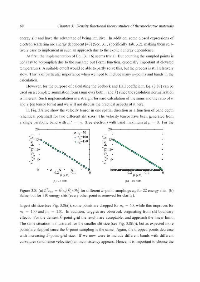
60 Chapter 3. Density functional theory studies of thermoelectric materials
energy slit and have the advantage of being intuitive. In addition, some closed expressions ofelectron scattering are energy dependent [48] (Sec. 3.1, specifically Tab. 3.2), making them rela-tively easy to implement in such an approach due to the explicit energy dependence.
At first, the implementation of Eq. (3.116) seems trivial. But counting the sampled points isnot easy to accomplish due to the smeared out Fermi function, especially important at elevatedtemperatures. A suitable cutoff would be able to partly solve this, but the process is still relativelyslow. This is of particular importance when we need to include many �k–points and bands in thecalculation.
However, for the purpose of calculating the Seebeck and Hall coefficient, Eq. (3.87) can beused on a complete summation form (sum over both n and �k) since the resolution normalizationis inherent. Such implementation is a straight forward calculation of the sums and the ratio of σ
and χ (on tensor form) and we will not discuss the practical aspects of it here.In Fig. 3.8 we show the velocity tensor in one spatial direction as a function of band depth
(chemical potential) for two different slit sizes. The velocity tensor have been generated froma single parabolic band with m∗ = me (free electron) with band maximum at μ = 0. For the
-0.2 -0.1 0μ [eV]
0
5
10
15
20
h2v xv x/(2
π)2 [e
V2 Å
2 ] nk=50nk=100nk=150
(a) 22 slits
-0.2 -0.1 0μ [eV]
0
5
10
15
20
h2v xv x/(2
π)2 [e
V2 Å
2 ]
(b) 110 slits
Figure 3.8: (a) h2vxx = ∂2εn(�k)/∂k2x for different �k–point samplings nk for 22 energy slits. (b)
Same, but for 110 energy slits (every other point is removed for clarity).
largest slit size (see Fig. 3.8(a)), some points are dropped for nk = 50, while this improves fornk = 100 and nk = 150. In addition, wiggles are observed, originating from slit boundaryeffects. For the densest �k–point grid the results are acceptable, and approach the linear limit.The same situation is illustrated for the smaller slit size (see Fig. 3.8(b)), but as expected morepoints are skipped since the �k–point sampling is the same. Again, the dropped points decreasewith increasing �k–point grid size. If we now were to include different bands with differentcurvatures (and hence velocities) an inconsistency appears. Hence, it is important to choose the
3.4. Transport properties 61
right compromise between slit size and �k–point sampling, or to introduce additional routinesto fill in the missing points. For the band engineering section (Sec. 3.5) later we manuallymatched the band curvatures and the slit and �k–point resolution to avoid any significant problemsof wiggles or lack of point pickup. For the articles where the Seebeck coefficient have beencalculated we used the direct sum approach due to its simpleness and lack of these problems.
Based on random point interpolations routines such as Kriging (see for example the book byA. G. Journel and Ch. J. Huijbregts[55] for a discussion of this technique) or modified Shep-ard [56] it is possible to adapt this code to utilize on the go interpolations in each slit, thussignificantly increasing the flexibility and redundancy by removing the aforementioned prob-lems.
Calculation of the chemical potential
We also want to calculate the temperature dependence of the transport coefficients, but this is notstraight forward due to the temperature dependence of the chemical potential. However, we cancircumvent the problem by assuming that we have a closed system with a constant number ofelectrons N and utilize the Fermi function such that
N =1
Ω
∑n
∫2fn(�k)d�k,
=1
Ω
∑n
∫2
e(ε(�k)−μ(T ))/kbT + 1d�k. (3.118)
At a given temperature this equation can be solved for the chemical potential by a least squareapproach, or similarly for a given temperature and particle number. We choose the Newton–Raphson method [2] (Sec. 9.4) as it is simple and sufficiently fast and accurate for our purpose.
The important �k–point convergence
The energy slit method needs interpolation routines to be stable and tractable for a wide rangeof systems. We shall see that the calculation of the transport properties by utilizing the Boltz-mann equations is burdened by additional severe �k–point convergence problems related to thecalculation of the band structure and the velocities. To illustrate these problems we will usethe band structure and velocities for the SrZn2Sb2 compound. The band structure and veloc-ities are extracted from density functional calculations in VASP based on a PBE+U [57, 58]approach (see paper IV for calculation details). Even though this fails to produce the correctoverall band structure (see paper V), the point of this section is to show problems related to

62 Chapter 3. Density functional theory studies of thermoelectric materials
the �k–point convergence. We only present data for the Seebeck coefficient, but the convergenceproblems are similar for the separate σ and χ tensors. The tensor trace of the Seebeck coeffi-cient (αxx + αyy + αzz)/3 is used for the convergence tests. All post–interpolation of the bandstructure and velocities have been performed by the modified Sheppard interpolation [56]. Thisinterpolation technique has the ability of extracting random points and was chosen with the futurepossibilities of such randomness in mind (e.g. interpolation along paths and scattered domains).
100
150
200
250
300
350
α [μ
V/K
]
12x12x616x16x820x20x1024x24x1228x28x14
5 10 15 20carrier conc. [x 1019 cm-3]
100
150
200
250
300
350
α [μ
V/K
]
5 10 15 20carrier conc. [x 1019 cm-3]
28x28x1482x82x40136x136x66190x190x92244x244x118
a) b)
c) d)
Figure 3.9: Convergence tests of the Seebeck coefficient as a function of carrier concentrationfor SrZn2Sb2 at 300 K. In (a), (b) and (c) the convergence as a function of input �k–point grid(see legend) is given for three different interpolation schemes. (a) fills none, (b) four and (c)eight points between the original points in the input grid. The 28×28×14 input �k–point grid isinterpolated (see legend for final grid density) and compared in (c).
The severeness of the �k–point convergence is evident from Fig. 3.9, where the Seebeckcoefficient versus carrier concentration is investigated for different �k–point grid densities. Alltransport calculations were done at a fixed temperature of 300 K. In Fig. 3.9(a) no interpolationis performed and, as the input grid becomes increasingly dense, there is trace of a slow conver-gence. Post-interpolating the output band structure grids by four intermediate points betweenthe originals (Fig. 3.9(b)) immediately improves the convergence. Doubling the point filling inFig. 3.9(c) yield very similar results and thus indicate a clear convergence. The same behaviour

3.4. Transport properties 63
Table 3.1: SrZn2Sb2�k–points used for the Seebeck coefficient convergence tests. Input grid
points in the Brillouin zone (BZ) and the irreducible Brillouin zone (IBZ) are also listed.
Original Interpolated (intermediate points)Grid IBZ BZ 2 4 6 812×12×6 100 864 34×34×16 56×56×26 78×78×36 100×100×4616×16×8 213 2048 46×46×22 76×76×36 106×106×50 136×136×6420×20×10 396 4000 58×58×28 96×96×46 134×134×64 172×172×8224×24×12 667 6912 70×70×34 116×116×56 162×162×78 208×208×10028×28×14 1030 10976 82×82×40 136×136×66 190×190×92 244×244×118
is seen in Fig. 3.9(d), where a 28×28×14 band structure grid is interpolated with no, two, four,six and then eight intermediate points. The difference between the first two is substantial, butthen the results start to converge, suggesting four intermediate points as an acceptable compro-mise. It is worth pointing out from Table 3.1 that, to obtain such convergence a fairly aggressivescheme is needed. More precisely, even though we already fill the Brillouin zone with 10976 �k–points, we need to post–interpolate this to 1.2 million �k–points, or roughly an order of magnitudeincrease of points in one direction to observe convergence. For the most aggressive interpolationscheme a convergence within 1–2 μV/K is obtained.
Reasonable convergence was possible for the Seebeck coefficient as a function of the carrierconcentration. But, one should not instantly think that this convergence is universal for e.g. thetemperature dependence of the Seebeck coefficient for the same band structure grids and inter-polation schemes. In Fig. 3.10 a similar convergence test is given for the Seebeck coefficientas a function of the temperature. For the non–interpolated band structure grids in Fig. 3.10(a),no overall convergence can be observed, although, it is signs of converging Seebeck coefficientat higher temperatures. Interpolating the band structure grids in Fig. 3.10 with four intermedi-ate points yields clear signs of convergence. This convergence further improves for the mostaggressive eight intermediate point interpolation scheme (see Fig. 3.10(c) and 3.10(d)). Accept-able convergence within 5–10 μV/K is obtained for the most aggressive interpolation scheme,although notice that this is almost an order of magnitude larger than what was possible with thecarrier concentration tests under the same conditions.
For readers unfamiliar with density functional calculations and the computational resourcesneeded to do such dense calculations should know that for the 28×28×14 calculations it wasnecessary to use 32 processors with roughly 15GB of memory on each processor. And this ispart of the reason why we choose a simple system like the SrZn2Sb2 compound. Obtainingsuch dense grids for larger systems, like the 14–1–11 compounds or the β–Zn4Sb3 compound is

64 Chapter 3. Density functional theory studies of thermoelectric materials
0
50
100
150
200
250
300α
[μV
/K]
12x12x616x16x820x20x1024x24x1228x28x14
400 600 800 1000Temperature [K]
100
150
200
250
300
α [μ
V/K
]
400 600 800 1000Temperature [K]
28x28x1482x82x40136x136x66190x190x92244x244x118
a) b)
c) d)
Figure 3.10: Convergence tests of the Seebeck coefficient as a function of temperature forSrZn2Sb2. Fermi level is set at the top of the valence band. See Fig. 3.9 for additional details.
simply not possible. However, even though a dense grid is needed for the SrZn2Sb2 compound,case–by–case studies of the convergence is crucial for the system of interest and a warning to thereader is hereby given to carefully assess published results not discussing this.
It would be very beneficial to solve the aforementioned convergence problems, such that thiskind of transport calculations could be done for larger systems and maybe in the future also forsystems incorporating defects or other imperfections in the crystal.
A possible solution is a grid shift approach [59] currently under development in VASP5.X.The main idea is based on the irreducible Brillouin zone (IBZ) and shifts of this. In principlewe would like to utilize the IBZ wherever possible due to the performance benefits. However,figuring out an interpolation (or extrapolation) scheme that operates on the IBZ and implementthis into running density functional codes is not trivial. The method under development worksby shifting the whole IBZ as shown in Fig. 3.11 and utilize an interpolation and extrapolation ofthe plane wave coefficients based on the original IBZ. The new shifted IBZ is then diagonalizedand the velocities (or other observables) are calculated. Contrary to the current approach ofgenerating the densest possible input grid and applying post–interpolation, this approach hasthe potential of being more accurate (interpolation/extrapolation directly from the plane wave

3.4. Transport properties 65
coefficients) and it is expected to give a significant improvement of speed and memory usage.
Figure 3.11: Outline of an interpolation approach that utilize irreducible Brillouin zone (IBZ)grid–shifts. A cubic 3×3×1 (one to keep the two dimensionality of the figure) IBZ is shownfor simplicity. The black points and lines represent the original IBZ, while the blue and greenrepresent two different shifts. When all shifts are done, the IBZ is up sampled by two additionalintermediate points. Increasing the number of shifts, while decreasing the shift length wouldincrease the up sampling.
Even though this approach was initially intended for transport calculations it turns out itcould also be used to generate dense density of states, band structures and improve the slowconvergence of the optical properties (similar to the transport, due to the calculation of the mo-mentum operator operating on the plane wave functions).
To illustrate some preliminary results of this approach, the density of states of the elementalAl is given in Fig. 3.12. Four base �k–point grids are calculated; 7×7×7, 11×11×11, 33×33×33and 55×55×55, respectively. Then, the base 11×11×11 grid is interpolated to a 33×33×33 anda 55×55×55 grid. The agreement between the interpolated 33×33×33 and the base 33×33×33grid is very good with the additional benefit of a significantly decreased computational time ascan be seen from Table 3.2. The calculation of the velocities currently suffer from a slight in-crease in computational time (but significant memory savings) due to dynamic symmetry lockups

66 Chapter 3. Density functional theory studies of thermoelectric materials
Table 3.2: Al density of states calculation times over a set of different �k–point grids. The base11×11×11 grid is interpolated to 33×33×33 and 55×55×55 �k–points using shifts of the irre-ducible Brillouin zone and interpolation/extrapolation of the plane wave coefficients.
Grid Time [s]11×11×11 2833×33×33 47055×55×55 197411×11×11→33×33×33 10011×11×11→55×55×55 189
needed for the explicit use of the IBZ. However, a linear to constant lockup with respect to thenumber of �k–points is expected when these routines are rewritten to utilize hashed �k–points. Thiswould yield a constant lockup time with some extra overhead (collision checks) compared to thecurrently unhashed routines. Consequently an order of magnitude speedup is expected. The ideaof using hash lockups is not new [60] (Chap. 6) and we will not discuss this further in this thesis.
3.5 Band engineering and the impact on the transport prop-erties
Now that a rigorous calculation of the transport properties can be done, let us investigate howdifferent band structure properties affect the electrical conductivity and the Seebeck coefficient.To do this in a consistent manner we generate fictitious bands based on the modified singleparabolic band approximation
ε(�k) =h2k2
2m∗+ Δε, (3.119)
where m∗ is the effective mass and Δε is an energy shift constant. The effective mass will set thecurvature of the band. The effective mass is replaced by m∗ = ame for simplicity. The constanta then determines the curvature of the band. A negative a generates a valence band, while apositive a yields a conduction band.
Before generating the bands it is worthwhile to investigate the different parameters that de-termine the electrical conductivity and the Seebeck coefficient. The electrical conductivity isfully determined by Eq. (3.98), while the Seebeck coefficient uses a combination of Eq. (3.98)and Eq. (3.99). While the relaxation time is of importance we will disregard it until further no-tice. The two remaining properties in the conductivity tensor are then the velocity tensor and the

3.5. Band engineering and the impact on the transport properties 67
0 10Energy [eV]
0
1
2
3
4
5
6
Den
sity
of s
tate
s [st
ates
/uni
t cel
l]7x7x711x11x1133x33x3355x55x5511x11x11 -> 33x33x3311x11x11 -> 55x55x55
5 7.5 101.5
2
Figure 3.12: Density of states for elemental Al for different sets of �k–point grids and interpo-lation schemes. The 11×11×11 grid has been interpolated to a 33×33×33 (green circles) anda 55×55×55 (indigo squares) grids to illustrate the potential of the shift approach. A Gaussiansmearing of 0.2 eV was added to the calculated results.
derivative of the equilibrium Fermi function. The velocities are dependent on the band structure(and quantum effects beyond what can be observed in the band structure), while the band pickupfrom the Fermi function derivative is only dependent on the temperature and the difference be-tween the energy and the chemical potential.
To illustrate the band pickup at different temperatures we plot ∂f/∂ε as a function of ε − μ
in Fig. 3.13(a), where the Fermi energy is set at zero. The derivative distribution is centered atμ, thus any shift of μ would shift the band pickup accordingly. The width of the distributionincreases with temperature as is well known from the Fermi function. For 300 K there is hardlyany band pickup outside ε − μ ± 0.2 eV, while there for 900K is significant pickup outside thisregion, dropping to zero at approximately ε − μ ± 0.5 eV. This tells us that the semi–classicalconductivity is determined (at all interesting temperatures) by states with energies in a regionof ±0.5 eV around the chemical potential. Due to the temperature dependent width of the bandpickup, the band velocities close to ε = μ are dominating at low temperatures, while at elevated

68 Chapter 3. Density functional theory studies of thermoelectric materials
temperatures, velocities away from ε = μ becomes increasingly more important.For the χ tensor the behavior is a bit more complicated. The main difference between the
pickup factor for χ and σ is an additional linear ε − μ weighting factor. In Fig. 3.13(b), where(ε − μ)∂f/∂ε is plotted as a function of ε − μ, this is clearly seen. The pickup as a function oftemperature is similar to that of the electrical conductivity, but is now multiplied by a linear term.The weighting amplitude is constant for all temperatures and the range pickup is slightly wider,especially at elevated temperatures. But the region of ±0.5 eV around μ is still valid. Because ofthe integral over the band pickup and velocity, the asymmetry of the χ band pickup leads to therequirement of band asymmetry around μ to obtain a large χ and thus a large Seebeck coefficient.If the bands are mirrored around μ within a large portion of the pickup region, χ would approachzero and thus yield a small Seebeck coefficient. If we assume that the velocity is constant (e.g.
-0.4 -0.2 0 0.2 0.4ε−μ [eV]
0
2
4
6
8
10
Wei
ghtin
g [e
V-1
]
T=300KT=500KT=700KT=900K
(a) Electrical conductivity band pickup
-0.4 -0.2 0 0.2 0.4ε−μ [eV]
-20
-10
0
10
20W
eigh
ting
[x 1
0-2]
(b) χ band pickup
Figure 3.13: (a) Band pickup for the σ (conductivity) tensor at four different temperatures. (b)Similar, but for the χ tensor. See (a) for legend.
isotropic structure with linear bands), the Seebeck coefficient is independent of the velocity. Forthe single band approximation we see that
v =hk
m∗, (3.120)
=
√2ε
m∗. (3.121)
Thus, for the single band approximation, the band pickup is multiplied by an additional√
ε factor.Due to the nature of the single band approximation it can immediately be recognized that the
electrical conductivity is easily calculated if the effective mass is known. It also turns out thatthe Seebeck coefficient is independent of the effective mass. Substituting the single parabolic

3.5. Band engineering and the impact on the transport properties 69
velocity Eq. (3.121) into Eq. (3.117) (and assuming a single band) the electrical conductivity σ
and the thermal coefficient χ are obtained for the single parabolic band approximation as follows
σs =e2
ΩkbT
√1
2h2m∗
∫ ∞
0
τ(ε)ε1/2
cosh((ε − μ)/kbT ) + 1dε, (3.122)
χs =e
ΩkbT 2
√1
2h2m∗
∫ ∞
0
τ(ε)ε1/2(ε − μ)
cosh((ε − μ)/kbT ) + 1dε, (3.123)
which from Eq. (3.91) gives the Seebeck coefficient
αs =1
eT
(∫ ∞
0τ(ε) ε3/2
cosh((ε−μ)/kbT )+1dε∫ ∞
0τ(ε) ε1/2
cosh((ε−μ)/kbT )+1dε
− μ
), (3.124)
where τ(ε) is an energy dependent scattering time. The way of maximizing the Seebeck coef-ficient from the single band approximation is if μ � ε or μ � ε. Another option would be tomake the denominator (conductivity) approach zero, which is satisfied for the same conditions.Hence, the longer away from the band μ is placed, the larger the Seebeck coefficient. This issomewhat fictitious since the conductivity would be zero and no current would be able to flow,but it illustrates the demand for asymmetry around μ to obtain the highest possible Seebeck co-efficient. The conductivity is increased by increasing the velocity (similar to a decrease of theeffective mass, or an increase of the band curvature).
To go beyond the single band approximation (but still in the parabolic approximation) wehave to sum over the additional bands in Eq. (3.122), (3.123) and (3.125). We will now leavethe single band approximation and perform band engineering to illustrate how the electrical con-ductivity and Seebeck coefficient varies over a wide range of band combinations. All transportcalculations in the rest of this thesis are based on the solution of the Boltzmann equation underthe approximations that lead to the Boltzmann transport equations in Sec. 3.4.4. These equa-tions are solved using the energy slit implementations presented in section Sec. 3.4.5. The bandcurvature is determined by the constant a, while the energy shift is determined by Δε. Unlessotherwise stated, the relaxation time have been taken to be independent of both energy and �k–points and fixed at 1 fs [9] (Chap. 1). For convenience the Fermi level εf is fixed at ε = 0, whereμ = εf at equilibrium.

70 Chapter 3. Density functional theory studies of thermoelectric materials
3.5.1 Chemical potential or carrier concentration
Studies of the transport properties are usually given as a function of carrier concentration orchemical potential. The carrier concentration is readily available from Hall measurements and itis thus more common to use carrier concentration representation when presenting experimentaldata. However, in this section we give most of the data versus the chemical potential due toits simpleness. But, for the constant scattering and energy filtered power factor we also includethe carrier concentration representation. The relation between chemical potential and carrierconcentration nc for a single parabolic band [9] (Chap. 28) is given by
nc(μ, m∗, T ) =
√2
π2
(m∗kbT
h2
)3/2 ∫ ∞
0
ε1/2f(ε, μ, T )dε. (3.125)
where f is the equilibrium Fermi distribution. This is calculated for illustrative purposes for aset of band curvatures in Fig. 3.14. It is important to emphasize that a sum over Eq. (3.126) isneeded if multiple bands are used.
-0.2 -0.1 0 0.1μ [eV]
1×10⁻⁶
1×10⁻⁵
1×10⁻⁴
1×10⁻³
1×10⁻²
n c [1021
cm
-3]
a=-0.5a=-1.0a=-1.5a=-1.0, -1.0a=-1.0, -0.5a=-0.5, -0.5
Figure 3.14: Carrier concentration as a function of chemical potential for a set of different effec-tive masses (band combinations). The absolute value of the effective mass parameter a is used inthe calculation of Eq. (3.126). The temperature is fixed at 300 K.

3.5. Band engineering and the impact on the transport properties 71
3.5.2 Temperature
To explicitly illustrate the temperature dependence of the band pickup we calculate the electricalconductivity and the Seebeck coefficient as a function of μ for different temperatures. The va-lence band is fixed at a = −1, Δε = 0 and thus resemble the free electron mass for simplicity.
-0.2 0 0.2μ [eV]
0
1
2
3
4
5
6
σ [M
Sm-1
]
T=300KT=500KT=700KT=900K
(a) Electrical conductivity
-0.2 0 0.2μ [eV]
0
0.5
1
1.5
α [m
V/K
]
(b) Seebeck coefficient
Figure 3.15: (a) Electrical conductivity and (b) Seebeck coefficient as a function of chemicalpotential at four different temperatures. See (a) for legend.
From Fig. 3.15 the increased band pickup is clearly illustrated at elevated temperatures.The fact that the Seebeck coefficient in Fig. 3.15(b) is largest when the band pickup decreases isvisible and due to the width of the pickup (and thus smaller conductivity), the Seebeck coefficientat room temperature at μ = 0.3 eV is largest of all four. At higher temperature a decreasedslope of the Seebeck coefficient as a function of μ is observed. This is caused by differentband pickup between σ and χ as illustrated in Fig. 3.13(a) and Fig. 3.13(b). This behaviouris cancelled between χ and σ at μ = 0, where the asymmetry is equal for all temperatures.However, for μ = 0 the symmetry changes due to the band pickup and the curves start to separate.To summarize;
• μ > 0; lower temperatures give higher Seebeck coefficients with the largest slope due toa small denominator (conductivity). The electrical conductivity is small due to the lack ofband pickup (except close to μ = 0).
• μ < 0; higher temperatures give higher Seebeck coefficients. The electrical conductivityat different temperatures becomes similar when μ enter the deeper regions of the band dueto the band pickup around μ.

72 Chapter 3. Density functional theory studies of thermoelectric materials
3.5.3 Curvature
In the previous section we underlined temperature dependent features of the electrical conductiv-ity and Seebeck coefficient. We now fix the temperature (in this case at 300 K) and investigate thecurvature of single parabolic bands (both valence and conduction), but postpone the discussionof the combination until a later section.
The electrical conductivity is proportional to the band curvature. From Fig. 3.16(a), we seethat bands with larger velocity results in an increased electrical conductivity. The difference of avalence band and conduction band is also shown for the band curvatures a = −1.0 and a = 1.0,respectively. The difference is just what we would expect, symmetric around μ = 0.
-0.2 0 0.2μ [eV]
0
2
4
6
8
10
12
σ [M
Sm-1
]
a=-1.5a=-1.0a=-0.5a=1.0
(a) Electrical conductivity
-0.2 0 0.2μ [eV]
-1
-0.5
0
0.5
1
α [m
V/K
]a=-1.5, a=-1.0, a=-0.5a=1.0
(b) Seebeck coefficient
Figure 3.16: (a) Electrical conductivity and (b) Seebeck coefficient as a function of chemicalpotential for four different band curvatures, determined by the constant a. The temperature isfixed at 300 K.
In Fig. 3.16(b) we again (also Eq. (3.125)) see that the Seebeck coefficient is independentof a change in the band curvature (effective mass), except for the obvious valence to conductionband changes. Negative Seebeck coefficients are a signature of positive band curvature, such thatn–doped materials will exhibit negative Seebeck values, while the opposite is true for p–dopedmaterials. Hence;
• Increasing the band curvature increases the conductivity, while the sign of the curvaturedetermines whether the conductivity increases for positive or negative μ.
• The Seebeck coefficient does not depend on the band curvature within the single parabolicband approximation. A sign change of the curvature changes the sign and the increas-ing/decreasing behaviour versus μ of the Seebeck coefficient.

3.5. Band engineering and the impact on the transport properties 73
3.5.4 Degeneracy and reciprocal shift
It is now time to determine how the electrical conductivity and the Seebeck coefficient respondto band degeneracy and shifts in reciprocal space. From the implementation of the energy slitsit should be obvious that any reciprocal shift does not matter as long as the band edges areretained within the pickup region. The changes of the electrical conductivity due to degeneracyare shown in Fig. 3.17(a), while they for the Seebeck coefficient are shown in Fig. 3.17(b). Thedifference between a single band and two bands is evident for the conductivity. By adding asecond band with a smaller effective mass, the electrical conductivity increases as is expectedfrom the additive behaviour of the bands and the direct dependence of the effective mass.
Any additional band (as long as it is not energy shifted with respect to the others) will how-ever not change the Seebeck coefficient. This is due to the cancellation effect between χ and σ
for a constant change in band curvature. Similar to the electrical conductivity, there is also nochange if we apply a reciprocal shift to one of the bands. The cancellation effect is a featureof the parabolic band approximation and can also be seen from Eq. (3.125). To summarize thissection;
-0.2 0 0.2μ [eV]
0
5
10
15
20
σ [M
Sm-1
]
a=-1.0a=-1.0, -1.0a=-1.0, -0.5
(a) Electrical conductivity
-0.2 0 0.2μ [eV]
0
0.5
1
1.5
α [m
V/K
]
(b) Seebeck coefficient
Figure 3.17: (a) Electrical conductivity and (b) Seebeck coefficient as a function of chemicalpotential, compared for one band, two bands similar curvatures and a two band case with differentcurvatures. The temperature is fixed at 300 K. See (a) for legend.
• The electrical conductivity is dependent on the band degeneracy. A doubling of the degen-eracy accordingly doubles the electrical conductivity if the bands are kept equal.
• The Seebeck coefficient is independent of the degeneracy in the parabolic approximation(as long as the bands are not energy shifted). Deviations in real systems are expected due

74 Chapter 3. Density functional theory studies of thermoelectric materials
to the failure of the parabolic approximation.
3.5.5 Energy shift
We have so far not investigated the effect of energy shifts of the generated bands. To investigatethis we use sets of single parabolic bands with different effective masses and energy shifts. InFig. 3.18(a) we see that a negative energy shift lowers the onset for band pickup and thus lowersthe onset of electrical conductivity. By introducing an additional band with the same curvature,but energy shifted from the original, the electrical conductivity increases accordingly as we sawin the previous discussion, although with a modification due to the later band pickup of theshifted band. Again, changes in the effective mass follows the previous discussions. However,for the Seebeck coefficient in Fig. 3.18(b) we see that the largest difference is introduced by thesingle band energy shifts. As previously discussed the Seebeck coefficient is largest where theconductivity drops to zero. It is also important to notice that it is the first band that dominatethe Seebeck coefficient. The introduction of additional bands deeper in energy only modify theSeebeck coefficient in the band pickup region of the additional band. An interesting fact to noteis the subtle difference in the Seebeck coefficient between the a = −1.0,−0.5, Δε = 0,−0.1
eV and a = −1.0,−0.5, Δε = −0.1, 0 eV calculations (see inset in Fig. 3.18(b)). The latter willhave a slightly higher electrical conductivity in the region from -0.1 to 0 eV, which yields a lowerSeebeck coefficient close to and in this region. The impact of energy shifts can be summarized
-0.2 0 0.2μ [eV]
0
5
10
15
20
σ [M
Sm-1
]
a=-1.0a=-1.0, Δε=-0.1 eVa=-1.0, Δε=-0.2 eVa=-1.0. -1.0a=-1.0, -1.0, Δε=0, -0.1 eVa=-1.0, -0.5, Δε=0, -0.1 eVa=-1.0, -0.5, Δε=-0.1, 0 eVa=-0.5, -0.5, Δε=0, -0.1 eV
(a) Electrical conductivity
-0.2 0 0.2μ [eV]
0
1.5
3
4.5
α [m
V/K
]
-0.2 -0.1 00
0.1
0.2
(b) Seebeck coefficient
Figure 3.18: (a) Electrical conductivity and (b) Seebeck coefficient as a function of chemicalpotential, compared for one band with and without energy shifts and two bands with differentcurvatures and energy shifts. The temperature is fixed at 300 K and the energy shift is given byΔε. See (a) for legend.

3.5. Band engineering and the impact on the transport properties 75
as follows;
• The electrical conductivity as a function of chemical potential changes drastically betweenthe different energy shifts. The largest conductivity is found for the band combination withthe lowest effective mass (largest band curvature).
• The Seebeck coefficient is highly dependent on the first band. Additional bands introducesmall (but still important) modifications in the respective pickup regions.
3.5.6 Conduction band
Even though the previous discussions are important, they are somewhat artificial. In most realis-tic situations, particularly at high temperate and in narrow band gap systems, conduction bandswill contribute. In Fig. 3.19(a) the electrical conductivity is given as a function of chemicalpotential for different combinations of valence and conduction bands. The previous discussionof the change in the conductivity as the effective mass changes still holds, although with addi-tional contributions on the conduction side. When the conduction band is pulled down into thevalence region to generate a metal–like system there is a non–zero region of the conductivity inthe overlap region between the valence and conduction bands. This even occurs for bands sepa-rated by a small gap (because of the distribution at 300 K). The Seebeck coefficient is similarly
-0.2 0 0.2μ [eV]
0
5
10
15
20
25
σ [M
Sm-1
]
a=-1.0a=-1.0, 1.0, Δε=0, 0.2 eVa=-1.0, 1.0, Δε=0, 0.1 eVa=-1.0, 1.0a=-1.0, 1.0, Δε=0, -0.1 eVa=-1.0, 0.5, Δε=0, 0.1 eVa=-0.5, 0.5, Δε=0, 0.1 eVa=-0.5, 0.5, Δε=0, -0.1 eV
(a) Electrical conductivity
-0.2 0 0.2μ [eV]
-0.5
0
0.5
1
α [m
V/K
]
(b) Seebeck coefficient
Figure 3.19: (a) Electrical conductivity and (b) Seebeck coefficient as function of chemical po-tential, compared for different combinations of a (negative is valence, positive is conduction)and energy shifts. The temperature is fixed at 300 K and the energy shift is given by Δε.
illustrated in Fig. 3.19(b). Here, we start to see many of the commonly known behaviours of theSeebeck coefficient for semi–conductors. For example, introducing a conduction band with the

76 Chapter 3. Density functional theory studies of thermoelectric materials
same effective mass as the valence band, separated by a small band gap gives a transition regionin the middle of the gap. In this region, the Seebeck coefficient changes sign from positive tonegative when the conduction band starts to dominate (or opposite for the valence band). A neg-ative Seebeck coefficient is associated with n–type behaviour, while p–type is positive. Whenthe gap decreases, the maximum and minimum Seebeck coefficient decreases due to the lack ofasymmetry around μ. Again, we see that an effective mass change is ignored if there is an equalchange between the conduction and valence band. A decrease of the effective mass in the con-duction band with respect to the valence band (or vice versa) results in a decrease of the Seebeckcoefficient due to the increased conductivity. To summarize;
• Introducing conduction bands does not modify the original discussion about the electri-cal conductivity. However, due to the change in sign of the effective mass, we also getconductivity contribution for positive μ. At a sufficiently wide gap (depending on the tem-perature), there is a region of zero conductivity in the gap region. This disappears whenthe thermal band pickup enclose the gap (e.g. high temperatures and/or small gap). A clearmetallic behaviour is then observed.
• The effect of conduction bands on the Seebeck coefficient is significant. A negative See-beck coefficient is to be associated with n–doped systems, while a p–type is to be associ-ated with the positive counterpart. The transition between a positive and negative Seebeckcoefficient takes place in the middle of the gap region if the valence and conduction bandsare symmetric around the gap with a sign change. A small band gap accordingly give asmall Seebeck coefficient due to less antisymmetry around μ.
3.5.7 Modifications due to electron scattering
Due to the non–cancelling relaxation time τ from σ, it is somewhat artificial to fix the scatteringtime without considering basic electron scattering. If we simply set τ to a constant, we get aconductivity that is increasing with increasing number of bands. Hence, the conductivity wouldkeep rising monotonically as the temperature is increased. For real systems this is highly un-physical and we need to introduce a parametrization for the relaxation time to account for at leastthe majority of effects.
The two dominating scattering mechanisms in doped semi–conductors are scattering byacoustical phonons and impurities. Simple models for both are given by Fistul [48] (Tab. 3.2). Inthis thesis we have implemented a factor similar to the one given in Eq. (3.2.22) of Fistul [48].

3.5. Band engineering and the impact on the transport properties 77
To summarize, Fistul defines
τa,i = τa0
|ε|3/2
|ε|2 + ξ2, (3.126)
whereξ2 =
τa0
τ i0
, (3.127)
as a relaxation time that contains both scattering by acoustical vibrations and impurities throughτa0 and τ i
0, respectively. Here, ξ2 gives the ratio between the acoustical and impurity contributions.The prefactor τa
0 is given as
τa0 =
9
4√
2
h4ω2M
C2a2(m∗kbT )3/2, (3.128)
where C is a Bloch constant, ξ the lattice parameter, ω the sound velocity, a the lattice parameterand M the atomic mass. We take τa
0 to be constant in energy. Hence, τa,i is a function of energyand ξ2 only. Substituting Eq. (3.127) into the transport equations, we see that τa
0 cancels forthe Seebeck and Hall coefficients, while it is retained for the electrical and thermal conductivity.The cancellation is convenient due to the complex problem of calculating τa
0 from ab–initioprinciples. Common relaxation times are in the order of tenths of femtoseconds [9] (Chap. 1).To simplify the comparisons we will fix τa
0 at 1 fs.
-0.2 0 0.2μ [eV]
0
5
10
σ [M
Sm-1
]
ξ=0.001ξ=0.01ξ=0.1ξ=1.0
(a) Electrical conductivity
-0.2 0 0.2μ [eV]
0
0.5
1
1.5
α [m
V/K
]
(b) Seebeck coefficient
Figure 3.20: (a) Electrical conductivity and (b) Seebeck coefficient as function of chemical po-tential, compared for different combinations of the scattering parameter ξ. Only one valenceband with a = −1 is included in the calculation. The temperature is fixed at 300 K. See (a) forlegend.
A large ξ means that τa0 >> τ i
0, thus primarily ionic scattering. For a small ξ the oppositeis true. The combined approach of Eq. (3.129) is difficult to compare to a constant scatteringtime used until now. This is due to the energy dependence (that modify the band pickup) and

78 Chapter 3. Density functional theory studies of thermoelectric materials
quantitative comparisons with the previous results will not be done.In Fig. 3.20 we compare results given different scattering parameters ξ for the electrical
conductivity and Seebeck coefficient. One valence band with a = −1 has been included in thecalculations. A scattering parameter of ξ = 1 clearly yields the largest dampening of the conduc-tivity and hence the largest Seebeck coefficient. Also, the curvature of the electrical conductivitychanges quite drastically from ξ = 1 to ξ = 0.001, the transition from combined ionic andacoustic to predominantly acoustic scattering. It is interesting to note the rather small change ofthe Seebeck coefficient (compared to the electrical conductivity), which is a consequence of thecancellation between the χ tensor and the electrical conductivity. There is however a constantshift of the Seebeck coefficient for the different scattering parameters.
-0.2 0 0.2μ [eV]
0
5
10
σ [M
Sm-1
]
ξ=0.001ξ=0.01ξ=0.1ξ=1.0
(a) Electrical conductivity
-0.2 0 0.2μ [eV]
-0.5
0
0.5α
[mV
/K]
(b) Seebeck coefficient
Figure 3.21: (a) Electrical conductivity and (b) Seebeck coefficient as function of chemical po-tential, compared for different combinations of the scattering parameter ξ. One valence band andone conduction band with a = −1, Δε = 0 eV and a = 1, Δε = 0.1 eV are included in thecalculation. The temperature is fixed at 300 K. See (a) for legend.
Introducing a shifted conduction band in Fig. 3.21 yields similar results, although with ad-ditional features. Due to the conduction band, a transition from n–type to p–type and the signchange in the Seebeck coefficient are observed. As before, the smallest conductivity gives thelargest Seebeck coefficient.
We can briefly summarize the scattering section in a few points;
• Scattering due to ionic impurities and acoustic vibrations scattering alters the electricalconductivity significantly.
• In this simple model, ionic scattering is the strongest electron scatter process.

3.5. Band engineering and the impact on the transport properties 79
• Changes in the Seebeck coefficient due to scattering are less significant than the changesobserved for the electrical conductivity. The behaviour as a function of chemical potential(and carrier concentration) is fairly similar, but a constant shift is applied.
• The difference between the one and two band model is similar to the previous discussiondisregarding scattering mechanisms.
3.5.8 Power factor and optimization of electronic properties
It should from the proceeding discussions be apparent that we can not simultaneously obtaina large electrical conductivity and a Seebeck coefficient. To obtain a large zT value, this isprecisely what is needed. The combination enters in the power factor p = α2σ in Eq. (2.4).Hence, for thermoelectric optimization, knowledge about this factor is crucial. We will in thissection discuss the compromise between the electrical conductivity and the Seebeck coefficientand how to obtain the “optimal” power factor.
Power factor with constant scattering
Let us first consider the power factor in absence of energy dependent scattering with a constantscattering time of 1 fs [9] (Chap. 1). In Fig. 3.22(a) we give the power factor as a function of thechemical potential for different combinations of bands. The maximum power factor is clearlyobtained for bands with the smallest effective mass (largest conductivity). The introduction of anadditional valence band with a = −0.5 increases the power factor, but when a is increased thepower factor approach the limit of the original band (compare green solid, dashed and dotted linesto the black solid line in Fig. 3.22). Similar behaviour is seen for the power factor as a functionof carrier concentration (only shown for valence bands) in Fig. 3.22(b). This is a very importantobservation that confirms that a small effective mass is essential for large power factors. Thepower factor is thus strongly dependent on the electrical conductivity and optimization of thisshould be a primary concern as long as a decent Seebeck coefficient is met in a given system.The addition of a conduction band introduces a second peak and has a relatively small effect onthe peak associated with the valence band. Another interesting observation is the shift of thevalence peak if one valence band is downshifted in energy (compare solid purple and green linein Fig. 3.22). This is accompanied by an increase of the peak width at a cost of the height andindicates that the range of operational temperature might be increased by filling the valence (orconduction if n–type is wanted) region with several similar, but energy shifted bands.

80 Chapter 3. Density functional theory studies of thermoelectric materials
-0.2 0 0.2
μ [eV]
0
20
40
60
80p
[mW
K-2
m-1
]
(a) As a function of chemical potential
1×10⁻⁸ 1×10⁻⁶ 1×10⁻⁴
nc [x 1021 cm-3]
0
20
40
60
80
p [m
WK
-2m
-1]
a=-0.5, 1.0, Δε=0, 0.2 eVa=-0.5, 1.0, Δε=0, 0.4 eVa=-0.5, -0.5, Δε=0, -0.1 eVa=-0.5, -0.5a=-0.5, -1.0a=-0.5, -1.5a=-0.5a=-1.0a=-1.5
(b) As a function of carrier concentration
Figure 3.22: (a) The power factor and as a function of the chemical potential and (b) carrierconcentration, compared for different combinations of bands given by the curvature a and theenergy shift Δε. The temperature is fixed at 300 K. See (b) for legend.
Power factor with energy dependent scattering
In the last section we discovered that the power factor was strongly dependent on the conduc-tivity (or more directly, the effective mass). Due the sensitivity of the electrical conductivity toscattering it is expected that the power factor will change significantly when electron scatteringis involved. In Fig. 3.23(a), 3.23(b) and 3.23(c) the power factor for three different scatteringparameters ξ = 0.01, 0.1 and 1.0 is given.
The result of ionic and acoustical scattering (ξ = 1.0) can be understood from Fig. 3.21(a).The slope and magnitude of the electrical conductivity are significantly changed, while the See-beck coefficient remains virtually unchanged. Thus, as a consequence, the peak of the powerfactor is downshifted and decreased due to the slope and magnitude changes of the electrical con-ductivity. A more subtle change is the similarity between the energy shifted calculation (solidindigo line) and the non–shifted calculation (solid green line) for larger ξ. One might expectthese changes to be similar to the constant scattering calculations in Fig. 3.22. However, due tothe modification in the band pickup (additional energy terms from τa,i) there is less change whenthe scattering model is applied.
When acoustical scattering becomes more important (ξ = 0.1) we see that the shift anddecrease of the valence peak is smaller. And, when the acoustic scattering is predominant(ξ = 0.01) we retain similar behaviour to the constant scattering time approach, except for themodification of the band pickup, causing a different behaviour of the shifted band. An increaseof the power factor is seen due to the increase of the total scattering time. All these changes can

3.5. Band engineering and the impact on the transport properties 81
-0.2 0 0.20
25
50
75
100
125
Pow
er fa
ctor
[mSV
2 K-2
m-1
]a=-0.5a=-1.0a=-1.5a=-0.5, 1.0, Δε=0, 0.2 eVa=-0.5, 1.0, Δε=0, 0.4 eVa=-0.5, -0.5, 1.0, Δε=0, 0, 0.2 eVa=-0.5, -1.0, 1.0, Δε=0, 0, 0.2 eVa=-0.5, -1.5, 1.0, Δε=0, 0, 0.2 eVa=-0.5, -0.5, 1.0, Δε=0, -0.1, 0.2 eV
-0.2 0 0.2μ [eV]
0
10
20
30
40
50
Pow
er fa
ctor
[mSV
2 K-2
m-1
]
-0.2 0 0.2μ [eV]
0
2
4
6
8
10
12
a)
b) c)
Figure 3.23: The power factor as a function of the chemical potential, compared for differentcombinations of bands given by the curvature a and the energy shift Δε. The temperature isfixed at 300 K. Scattering parameters are ξ = 0.01, 0.1, 1.0 for (a), (b) and (c), respectively.
be explained from the electrical conductivity in Fig. 3.21(a).
3.5.9 Figure–of–merit
The previous section discussed band dependencies of the power factor. A strong correlationbetween the velocity (electrical conductivity) and power factor was shown. However, the figure–of–merit, zT also depends on the electrical and lattice thermal conductivities. From Eq. (2.4) wecan separate these thermal conductivities such that
zT =α2σ
κe + κl
T, (3.129)
where κe and κl are the electrical and lattice thermal conductivities, respectively. By rewritingEq. (3.130) we get
zT =α2σ(
1 + κl
κe
)κe
T. (3.130)
82 Chapter 3. Density functional theory studies of thermoelectric materials
Through Wiedemann-Franz law [61]κe = L0Tσ, (3.131)
where L0 is the Sommerfield Lorentz constant [9] (Chap. 1), we obtain
zT =α2
L0
(1 + κl
κe
) . (3.132)
Generally, L0 should be replaced by a Lorentz function L, which can is calculated from theratio between the electrical conductivity and the electrical thermal conductivity tensors. This isclearly shown in Fig. 3.24 for different band combinations. Unless the valence bands are shiftedwith respect to each other, they do not alter the one band behaviour of the Lorentz function. Asmall difference between the energy shifted (purple diamonds) and the energy non-shifted (greencircles) Lorentz functions can be seen close to the shifted band onset. Adding a conduction bandpulls the Lorentz values down towards the L0 constant. In the metallic (or highly doped) limit,the Lorentz function approaches the commonly used L0 constant.
To illustrate the band curvature dependence of the figure–of–merit, we calculate the Lorentztensor and use its trace in Eq. (3.131) and give the figure–of–merit as a function of chemicalpotential and lattice thermal conductivity in Fig. 3.25 and 3.26. From this it is clear that alarge band curvature and low lattice thermal conductivity are needed to obtain a large zT value.Additional bands increase the zT value further and if they are shifted with respect to each other,a slight increase of the width of the zT peak at the cost of height is observed (similar to thepower factor). A conduction band yields what is expected, another zT peak associated with it,where the separation between the center zT valence and conduction peak is determined by thethe band gap. For a sufficiently large gap the single band zT valence peak is retained. However,by pulling the conduction band into the valence region the zT peak decreases drastically eventhough the band curvature is large. Notice that the zT value is largest right above the valenceband edge onset. Unfortunately this is a region which is difficult to reach, but the closer we are tothe termination of the band from below (valence bands), the larger the zT value is, demonstratingalso the need for asymmetry.
We can thus summarize;
• By lowering the lattice thermal conductivity, the zT value increases.
• Increasing the band curvature and/or degeneracy increases the zT value.
• Asymmetry around μ is necessary for a large zT value and the chemical potential should

3.5. Band engineering and the impact on the transport properties 83
be set close to the band onset in the given temperature range.
• The operational temperature might be improved by adding several bands with sufficientspacing so that continues asymmetries exist for decreasing (increasing for n-type) chemicalpotential.
-0.2 0 0.2μ [eV]
0.01
0.1
1
10
L [μ
V2 /K
2 ]
a=-0.5, 1.0, Δε=0, 0.2 eVa=-0.5, 1.0, Δε=0, 0.4 eVa=-0.5, -0.5, Δε=0, -0.1 eVa=-0.5, -0.5a=-0.5L0
Figure 3.24: Lorentz function for different combinations of bands given by the curvature a andthe energy shift Δε. Temperature is fixed at 300K. The Sommerfield Lorentz number L0 is alsoshown for comparison.
3.5.10 Energy filtering
Albeit this might seem artificial, there is a possible way to increase the power factor beyondthe classical approach. What if we introduce an energy barrier that modifies the band pickup?This would increase or decrease the asymmetry around μ and thus modify the Seebeck coefficientsignificantly. At the same time, the electrical conductivity should also change (within the filteringregion), but opposite to the Seebeck coefficient, thus leading to a possible large change in thepower factor. Such a barrier could arise from e.g. scattering. For modelling purposes we chose
84 Chapter 3. Density functional theory studies of thermoelectric materials
here a scattering time relaxation to be represented by a Heavyside step function H(−ε−εb) timesa constant scattering time. By using this function an energy filtered band pickup is generated suchthat only states with larger energy than the barrier is allowed to be involved in the transport. Thereason for choosing such simple function is purely due to implementation reasons and for morerealistic calculations it would be beneficial to introduce a more complicated filter function (e.g.at least a Gaussian smeared Heavyside function). We now define the energy dependent scatteringtime as
τ(ε) = τ0H(|ε| − εb), (3.133)
where τ0, ε and εb are the constant relaxation time, the energy and the energy barrier, respectively.The Heavyside step function is defined as
H(|ε| − εb) =
⎧⎪⎨⎪⎩
0 |ε| < εb
12
|ε| = εb
1 |ε| > εb
(3.134)
For simplicity we again fix τ0 at 1 fs [9] (Chap. 1). In Fig. 3.27 we compare the electricalconductivity and the Seebeck coefficient at different energy barriers and different combinationsof valence bands. The Seebeck coefficient is significantly enhanced by the introduction of anenergy barrier. Increasing the energy barrier further yields an even larger Seebeck coefficient.The electrical conductivity rapidly drops to zero in the region where the Heavyside function iszero, but approaches the unfiltered calculation away from the barrier onset.
Results of this are apparent when we look at the power factor as a function of chemicalpotential in Fig. 3.28(a). Close to a doubling of the power factor is observed when we introducean energy barrier in 0.1 eV steps. This change is dramatic. In Fig. 3.28(b) the power factoras a function of carrier concentration is plotted (only for the valence bands) and it is similarlybehaved as the results presented in Fig. 3.28(a).
To illustrate the change in the figure–of–merit due to energy filtering we give the zT value asa function of lattice thermal conductivity and chemical potential in Fig. 3.29 for three differentenergy filtering schemes, given by the energy barrier εb. Similarities between the changes dueto the energy filtering in the power factor and the zT value are observed. Notice that the energyfiltering shifts the zT peak to lower chemical potential, or higher carrier concentration. This isvery convenient, since the right size of filtering can tune the zT to the chemical potential thatyields the highest band curvature or to chemical potentials that can be reached in real samples.

3.5. Band engineering and the impact on the transport properties 85
3.5.11 Band structure requirements
In this section we will briefly summarize the band engineering sections by pointing out somekey requirements needed of the band structure to be able to obtain a large power factor andfigure–of–merit. Based on the previous discussions the reader should consider the following;
• Low effective masses (high velocity) are important (if not crucial)
• A high level of degeneracy is important (degeneracy in �k–space is equally valid)
• Decent Seebeck coefficient is important (asymmetry around μ)
• Depending on the operational range in temperature or chemical potential there is a com-promise between the electrical conductivity and the Seebeck coefficient. If an acceptableSeebeck coefficient is obtained, focus should be shifted towards maximizing the electronicconductivity.
• A wider operational temperature can be obtained (with a compromise of the peak powerfactor and figure–of–merit value) by shifting (or adding) similar bands with low effectivemass downwards (upwards if n–type) in the valence (conduction if n–type) band.
• When the “optimal” power factor is reached and there is little potential for improvement,energy filtering should be introduced to further improve the power factor. If an almostperfect step function can be made, it should be possible to increase the power factor by afactor of 2–4 (and accordingly the zT value).
• Energy filtering can potentially be used to tune the optimal figure–of-merit to a feasiblechemical potential and carrier concentration region.
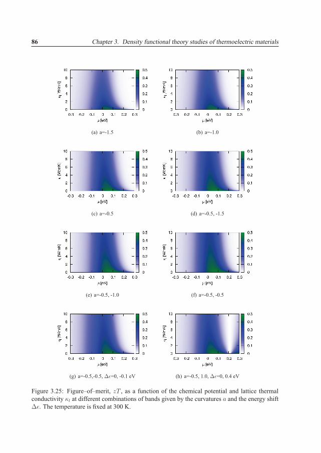
86 Chapter 3. Density functional theory studies of thermoelectric materials
(a) a=-1.5 (b) a=-1.0
(c) a=-0.5 (d) a=-0.5, -1.5
(e) a=-0.5, -1.0 (f) a=-0.5, -0.5
(g) a=-0.5,-0.5, Δε=0, -0.1 eV (h) a=-0.5, 1.0, Δε=0, 0.4 eV
Figure 3.25: Figure–of–merit, zT , as a function of the chemical potential and lattice thermalconductivity κl at different combinations of bands given by the curvatures a and the energy shiftΔε. The temperature is fixed at 300 K.

3.5. Band engineering and the impact on the transport properties 87
(a) a=-0.5, 1.0, Δε=0, 0.2 eV (b) a=-0.5, 1.0, Δε=0, -0.1 eV
Figure 3.26: Figure–of–merit, zT , as a function of the chemical potential and lattice thermalconductivity κl at different combinations of bands given by the curvatures a and the energy shiftΔε. The temperature is fixed at 300 K.
-0.2 0 0.2μ [eV]
0
2
4
6
8
10
12
σ [M
Sm-1
]
a=-1.0a=-1.0, εb=-0.1 eVa=-1.0, εb=-0.2 eVa=-1.0, -1.0, Δε=0, -0.1 eVa=-1.0, -1.0, Δε=0, -0.1 eV,εb=-0.1 eVa=-1.0, -1.0, Δε=0, -0.1 eV,εb=-0.2 eV
(a) Electrical conductivity
-0.2 0 0.2μ [eV]
0
0.5
1
1.5
2
α [m
V/K
]
(b) Seebeck coefficient
Figure 3.27: (a) Electrical conductivity and (b) Seebeck coefficient as function of chemical po-tential, compared for different combinations of the energy barrier εb. One valence band, a = −1,is included in the calculation. Data for the two band case is not shown due to the similarities tothe one band case (see previous discussions). The temperature is fixed at 300 K and the energyshift is Δε. See (a) for legend.

88 Chapter 3. Density functional theory studies of thermoelectric materials
-0.2 0 0.2μ [eV]
0
20
40
60
80
p [m
SV2 K
-2m
-1]
(a) As a function of chemical potential
1×10⁻⁶ 1×10⁻⁴ 1×10⁻²
nc [1021 cm-3]
0
20
40
60
80
p [m
SV2 K
-2m
-1]
a=-1.0, -1.0, Δε=0, -0.1 eVa=-1.0, -1.0, Δε=0, -0.1 eV,εb=-0.1 eVa=-1.0, -1.0, Δε=0, -0.1 eV,εb=-0.2 eVa=-1.0a=-1.0, εb=-0.1 eVa=-1.0, εb=-0.2 eV
(b) As a function of carrier concentration
Figure 3.28: (a) Power factor as function of the chemical potential and (b) carrier concentration,compared for different combinations of the energy barrier εb and bands. The temperature is fixedat 300 K and the energy shift is Δε. See (b) for legend.
(a) a=-1.0 (b) a=-1.0, εb=-0.1 eV
(c) a=-1.0, εb=-0.2 eV
Figure 3.29: Figure–of–merit, zT , as a function of the chemical potential and lattice thermalconductivity κl at a = −1.0 and different energy barriers εb. The temperature is fixed at 300 K.

References 89
References
[1] A. I. M. Rae. Quantum Mechanics. Taylor & Francis, 2002.
[2] W. H. Press, S. A. Teukolsky, W. T. Vetterling, and B. P. Flannery. Numerical Recipes 3rdEdition: The Art of Scientific Computing. Cambridge University Press, 2007.
[3] G. Meurant. The Lanczos and Conjugate Gradient Algorithms: From Theory to FinitePrecision Computations (Software, Environments and Tools). SIAM, 2006.
[4] P. Hohenberg and W. Kohn. Inhomogeneous electron gas. Phys. Rev., 136:B864, 1964.
[5] W. Kohn and L. J. Sham. Self-consistent equations including exchange and correlationeffects. Phys. Rev., 140:A1133, 1965.
[6] W. Pauli. Uber den zusammenhang des abschlusses der elektronengruppen im atom mit derkomplexstruktur der spektren. Z. Physik, 31:765, 1925.
[7] J. C. Slater. Atomic shielding constants. Phys. Rev., 36:57, 1930.
[8] S. F. Boys. Electronic wave functions. A general method of calculation for the stationarystates of any molecular system. Proc. R. Soc. London Ser. A, 200:542, 1950.
[9] N. W. Ashcroft and N. D. Mermin. Solid State Physics. Thomson Learning, 1976.
[10] D. J. Singh and L. Nordstrom. Planewaves, pseudopotentials, and the LAPW method. 2nded., Springer, New York, 2005.
[11] O. K. Andersen. Linear methods in band theory. Phys. Rev. B, 12:3060, 1975.
[12] P. E. Blochl. Projector augmented-wave method. Phys. Rev. B, 50:17953, 1994.
[13] G. Kresse and D. Joubert. From ultrasoft pseudopotentials to the projector augmented-wavemethod. Phys. Rev. B, 59:1758, 1999.
[14] M. Torrent, F. Jollet, F. Bottin, G. Zerah, and X. Gonze. Implementation of the projectoraugmented-wave method in the abinit code: Application to the study of iron under pressure.Comput. Mater. Sci., 42:337, 2008.
[15] J. P. Perdew and M. Levy. Physical content of the exact kohn-sham orbital energies: Bandgaps and derivative discontinuities. Phys. Rev. Lett., 51:1884, 1983.

90 Chapter 3. Density functional theory studies of thermoelectric materials
[16] J. P. Perdew, R. G. Parr, M. Levy, and J. L. Balduz Jr. Density-functional theory for frac-tional particle number: Derivative discontinuities of the energy. Phys. Rev. Lett., 49:1691,1982.
[17] W. Yang, Y. Zhang, and P. W. Ayers. Degenerate ground states and a fractional number ofelectrons in density and reduced density matrix functional theory. Phys. Rev. Lett., 84:5172,2000.
[18] A. J. Cohen, P. Mori-Sanchez, and W. Yang. Fractional charge perspective on the band gapin density-functional theory. Phys. Rev. B, 77:115123, 2008.
[19] P. Mori-Sanchez, A. J. Cohen, and W. Yang. Buried Ni/Cu(001) interface at the atomicscale. Phys. Rev. Lett., 100:146401, 2008.
[20] A. J. Cohen, P. Mori-Sanchez, and W. Yang. Fractional spins and static correlation error indensity functional theory. J. Chem. Phys., 129:121104, 2008.
[21] R. M. Dreizler and E. K. U. Gross. Density Functional Theory. Springer, Berlin, 1990.
[22] D. M. Ceperley and B. J. Alder. Ground state of the electron gas by a stochastic method.Phys. Rev. Lett., 45:566, 1980.
[23] R. Q. Hood, M. Y. Chou, A. J. Williamson, G. Rajagopal, and R. J. Needs. Quantum montecarlo investigation of exchange and correlation in silicon. Phys. Rev. Lett., 78:3350, 1997.
[24] R. Q. Hood, M. Y. Chou, A. J. Williamson, G. Rajagopal, and R. J. Needs. Exchange andcorrelation in silicon. Phys. Rev. B, 57:8972, 1998.
[25] J. P. Perdew, J. A. Chevary, S. H. Vosko, K. A. Jackson, M. R. Pederson, D. J. Singh,and C. Fiolhais. Atoms, molecules, solids, and surfaces: Applications of the generalizedgradient approximation for exchange and correlation. Phys. Rev. B, 46:6671, 1992.
[26] C. Fiolhais, F. Nogueira, and M. A.L. Marques. A primer in Density Functional Theory.Springer, Berlin, 2003.
[27] V. Fock. Naherungsmethode zur losung des quantenmechanischen mehrkorperproblems.Z. Physik, 61:126, 1930.
[28] M. Ernzerhof. Construction of the adiabatic connection. Chem. Phys. Lett., 263:499, 1996.

References 91
[29] M. Ernzerhof, J. P. Perdew, and K. Burke. Coupling-constant dependence of atomizationenergies. Int. J. Quantum Chem., 64:285, 1997.
[30] J. P. Perdew, M. Ernzerhof, and K. Burke. Rationale for mixing exact exchange with densityfunctional approximations. J. Chem. Phys., 105:9982, 1996.
[31] C. Adamo and V. Barone. Toward reliable density functional methods without adjustableparameters: The PBE0 model. J. Chem. Phys., 110:6158, 1999.
[32] J. Heyd, G. E. Scuseria, and M. Ernzerhof. Hybrid functionals based on a screened coulombpotential. J. Chem. Phys., 118:8207, 2003.
[33] M. Marsman, J. Paier, and G. Kresse. Hybrid functionals applied to extended systems. J.Phys.: Condens. Matter, 20:064201, 2008.
[34] J. Heyd and G. E. Scuseria. Efficient hybrid density functional calculations in solids: As-sessment of the heyd-scuseria-ernzerhof screened coulomb hybrid functional. J. Chem.Phys., 121:1187, 2004.
[35] E. N. Brothers, A. F. Izmaylov, J. O. Normand, V. Barone, and G. E. Scuseria. Accuratesolid-state band gaps via screened hybrid electronic structure calculations. J. Chem. Phys.,129:011102, 2008.
[36] J. P. Glusker, M. Lewis, and M. Rossi. Crystal Structure Analysis for Chemists and Biolo-gists. Wiley-VCH, 1994.
[37] P. Wilkes. Solid State Theory in Metallurgy. Cambridge University Press, London, 1973.
[38] L. Wu, Y. Zhu, T. Vogt, H. Su, J. W. Davenport, and J. Taftø. Valence-electron distributionin MgB2 by accurate diffraction measurements and first-principles calculations. Phys. Rev.B, 69:064501, 2004.
[39] A. P. Grosvenor, R. G. Cavell, and A. Mar. X-ray photoelectron spectroscopy study of theskutterudites LaFe4Sb12, CeFe4Sb12, CoSb3, and CoP3. Phys. Rev. B., 74:125102, 2006.
[40] H. Anno, K. Matsubara, T. Caillat, and J.-P. Fleurial. Valence-band structure of the skutteru-dite compounds CoAs3, CoSb3, and RhSb3 studied by x-ray photoelectron spectroscopy.Phys. Rev. B., 62:10737, 2000.

92 Chapter 3. Density functional theory studies of thermoelectric materials
[41] J. Graetz, C. C. Ahn, H. Ouyang, P. Rez, and B. Fultz. White lines and d-band occu-pancy for the 3d transition-metal oxides and lithium transition-metal oxides. Phys. Rev. B.,69:235103, 2004.
[42] Ø. Prytz, J. Taftø, C. C. Ahn, and B. Fultz. Transition metal d-band occupancy in skutteru-dites studied by electron energy-loss spectroscopy. Phys. Rev. B., 75:125109, 2007.
[43] D. H. Pearson, C. C. Ahn, and B. Fultz. White lines and d-electron occupancies for the 3dand 4d transition metals. Phys. Rev. B., 47:8471, 1993.
[44] J. M. Zuo. Measurements of electron densities in solids: a real-space view of electronicstructure and bonding in inorganic crystals. Rep. Prog. Phys., 67:2053, 2004.
[45] J. M. Zuo, M. Kim, M. O’Keeffe, and J. C. H. Spence. Direct observation of d-orbital holesand Cu-Cu bonding in Cu2O. Nature, 401:49, 1999.
[46] G. A. Slack and V. G. Tsoukala. Some properties of semiconducting IrSb3. J. App. Phys.,76:1665, 1994.
[47] C. Uher. Skutterudites: Prospective novel thermoelectrics. Semiconductors and semimetals,69:139, 2001.
[48] V. I. Fistul. Heavily Doped Semiconductors. Translated from Russian by Albin Tybulewicz,published in English by Plenum Press, New York, 1969.
[49] R. C. Dorf. The Electrical Engineering Handbook, Second Edition. CRC, Boca Raton,1997.
[50] G. Kresse and J. Hafner. Ab initio molecular dynamics for open-shell transition metals.Phys. Rev. B, 48:13115, 1993.
[51] G. Kresse and J. Hafner. Ab initio molecular-dynamics simulation of the liquid-metal-amorphous-semiconductor transition in germanium. Phys. Rev. B, 49:14251, 1994.
[52] G. Kresse and J. Furthmuller. Efficiency of ab-initio total energy calculations for metalsand semiconductors using a plane-wave basis set. Comp. Mater. Sci., 6:15, 1996.
[53] G. Kresse and J. Furthmuller. Efficient iterative schemes for ab initio total-energy calcula-tions using a plane-wave basis set. Phys. Rev. B, 54:11169, 1996.

References 93
[54] M. Gajdos, K. Hummer, G. Kresse, J. Furthmuller, and F. Bechstedt. Linear optical prop-erties in the projector-augmented wave methodology. Phys. Rev. B, 73:045112, 2006.
[55] A. G. Journel and C. J. Huijbregts. Mining geostatistics. Academic press, London, 1978.
[56] R. J. Renka. Algorithm 661. qshep3d: Quadratic shepard method for trivariate interpolationof scattered data. ACM Trans. Math. Software, 14:151, 1988.
[57] J. P. Perdew, K. Burke, and M. Ernzerhof. Generalized gradient approximation made sim-ple. Phys. Rev. Lett., 77:3865, 1996.
[58] A. I. Liechtenstein, V. I. Anisimov, and J. Zaanen. Density-functional theory and stronginteractions: Orbital ordering in mott-hubbard insulators. Phys. Rev. B, 52:R5467, 1995.
[59] Discussions with Georg Kresse, 2008.
[60] D. Knuth. The Art of Computer Programming. Addison-Wesley, Massachusetts, 1998.
[61] G. Wiedemann and R. Franz. Ueber die warme-leitungsfahigkeit der metalle. Annalen derPhysik, 165:497, 1853.


Papers
We will here present the papers included in this thesis. All articles are based on density functionalcalculations and all, except the first paper also include experimental data to confirm or investigatemotivating questions of the papers further.
Paper I – Bond analysis of phosphorus skutterudites: elongatedlanthanum electron buildup inLaFe4P12
Status: Submitted to Computational Material Science, 29.06.2009
Authors: Espen Flage–Larsen, Ole Martin Løvvik, Øystein Prytz and Johan Taftø
Recently there have been much experimental and theoretical work regarding the correlatedmotion of the filler ions in the skutterudite structure. We thus wanted to investigate the chargesurroundings of the filler ions and intended to perform a strict electron charge analysis to geta better spatial view of the electronic structure close to the filler ions. However, such chargeanalysis is complicated by the lack of a well defined charge reference.
From a modelling point of view, we have the option of generating a procrystal containing asuperposition of free atomic electron densities. Such a procystal contains overlapping densities,but is by definition without bonds. The bonds can then be analysed and visualized from thedifference between the crystal and procrystal electron density.
We performed such an analysis for the phosphorus skutterudites CoP3 and LaFe4P12.All calculation, visualisations, most of the interpretation and the write up of the article was
done by Espen Flage–Larsen, while Ole Martin Løvvik assisted.

Paper II – The influence of exact exchange corrections in vander Waals layered narrow band gap black phosphorus
Status: Submitted to Journal of Physics: Condensed Matter, 11.08.2009
Authors: Øystein Prytz and Espen Flage–Larsen
Based on the development of new hybrid functionals for use in the density functional frame-work we wanted to do a comparison of these new functionals and how they performed in acombined covalent and van der Waals bond dominated structure. The van der Waals interactionis purely determined by long–range correlation forces and is not included in any of the tradi-tional functionals. However, it is well known that many of the DFT functionals include residueexchange couplings at long range, which effectively introduces an artificial bond in the van derWaals region. By the inclusion of Fock terms (exact exchange) this can be corrected such thatthe functional is free of van der Waals bonds.
The black phosphorus was chosen as a test case based on previous work on phosphorus inthe electron microscope. Also, the black phosphorus contains important covalent bonds thatneed to be handled correctly before a satisfactory agreement can be met with the experiments.In this work we obtained electron energy loss spectra (EELS) and compared them to real spacemultiple scattering (RSMS) and density functional theory (DFT) calculations. Even in the RSMScalculations most features except the band gap were accounted for. However, a dispersion inthe conduction band was lacking. Similar results were obtained using the standard functionals(PZ–LDA) and (PBE–GGA). When the hybrid functionals (HSE03 and PBE0) were applied asignificant dispersion was added together with an opening of a gap. Relaxation of the structurewas also done using the hybrid functionals, which gave indications that PBE0 was free of theexchange residue due to a non–converged and drifting inter–layer distance.
This paper is not following the red line of first–principle studies of thermoelectric materialsthat is the focus of this thesis. However, it is still included to demonstrate the importance ofinvestigating new functionals. In particular, the hybrid functionals will be of importance to manythermoelectric materials that contains d and f states close to the Fermi level (see for examplepaper V).
Øystein Prytz did the experimental work and the RSMS calculations, while Espen Flage–Larsen did the DFT part. The interpretation of the results and writeup of the article were a jointeffort.

Paper III – Electron energy loss spectroscopy of the L2,3 edge ofphosphorus skutterudites and electronic structure calculations
Status: Published in Physical Review B, 11.08.2009
Authors: Ragnhild Sæterli, Espen Flage–Larsen, Øystein Prytz, Johan Taftø, Knut Marthin-sen and Randi Holmestad
Ref: Phys. Rev. B 80, 075109 (2009)
Motivated for the same reasons as in the first paper we wanted to do a combined analysis ofelectron energy loss spectroscopy (EELS) and density functional calculations (DFT) to furtherinvestigate the phosphorus bonds. Experimental investigations of the phosphorus energy lossedges were lacking in the literature and data was acquired and compared to density functionalcalculations of the conduction density of states. A good agreement between experiments andcalculations was found. Real space multiple scattering (RSMS) calculations were also performedto calculate the EELS spectra directly. The agreement of the EELS spectra and RSMS calculationwas satisfactory.
The experimental work was done by Ragnhild Sæterli, DFT calculations were performed byEspen Flage–Larsen, and the RSMS calculations by Øystein Prytz. The writing of the article wasa collaboration between all three, although Ragnhild did much of the writing of the introductionand the interpretation of the experimental results.

Paper IV – Electronic structure and transport in thermoelec-tric compounds AZn2Sb2 (A = Sr, Ca, Yb, Eu)
Status: Submitted to Dalton Transactions, 14.07.2009
Authors: Eric S. Toberer, Andrew F. May, Brent Melot, Espen Flage–Larsen and JeffSnyder
The aim of this invited paper was to summarize previous work on the 122 Zintl compounds andput them into a larger thermoelectric context. In addition the thermoelectric properties of the (upuntil then undocumented) SrZn2Sb2 were included and analysed. The results was found to fitwell within the 122 context.
Thermoelectric measurements and synthesis were done by Eric Toberer, Andrew May andJeff Snyder. Density functional and transport calculations were done by Espen Flage–Larsen.Initial results of Brent Melot were reworked and charge analyses were added. The interpreta-tion of the thermoelectric properties was initially done by Eric Toberer and Andrew May withadditional interpretations and comments by Espen Flage–Larsen.
Paper V – Valence band study of thermoelectric Zintl SrZn2Sb2
and YbZn2Sb2
Status: Submitted to Physical Review B, 13.08.2009
Authors: Espen Flage–Larsen, Spyros Diplas, Eric S. Toberer and Andrew F. May
This paper sought to address several issues regarding the calculations in Paper IV. Due to theneed for a band gap of the SrZn2Sb2, a semi–empirical correction was added to be able to obtainreasonable transport properties. Based on previous discoveries and experience of Paper II, cal-culations using hybrid functionals were compared to the previous calculations in Paper IV andX–ray photoemission spectra. Excellent corrections of the Zn d peak, Yb f peak and band gapwere shown for the hybrid functionals. In addition, there have been some discussions in the liter-ature regarding additional inherent Yb3+ in the YbZn2Sb2. Due to non-existing density of statesfor the Yb2O3 (should nominally contain Yb3+) in the literature, this was calculated. However,these calculations did not reproduce the claimed Yb3+ region and it is thus an XPS effect due toYb 4d–4f resonances as previously indicated in literature. The YbZn2Sb2 sample was investi-gated as a function of in–situ Ar+ scattering before doing an XPS sweep. Significant reductionin the Yb3+ peaks was found. However, even after one hour of sputtering (unrealistically long)there were still signs of Yb3+ in the sample, either due to Yb2O3 in the sample (not only surface)or inherent Yb3+. Structure relaxation was then done for a 1×1×3 cell with three Yb layers andno forced symmetry. No significant deviation from the reported structure was found. In addi-tion, relaxation of the same cell, but with one Yb removed did not yield significant occupancychange to conclude that inherent Yb3+ was likely. However, these models were simple and largersuperstructure and defect models need to be considered before drawing conclusions.
Density functional calculations were performed by Espen Flage–Larsen, while Spyros Diplasobtained experimental X–ray photoemission spectra. Eric Toberer and Andrew May did thesample synthesis. The writeup and interpretations was mostly done by Espen Flage–Larsen withassistance of Spyros Diplas on the oxygen discussion.