Density and Mortality in a Harvested Population of Quahog...

Fisheries Assessment and Management in Data-Limited SituationsAlaska Sea Grant College Program • AK-SG-05-02, 2005

161

Density and Mortality in a Harvested Population of Quahog (Mercenaria mercenaria) in Nova Scotia, CanadaKevin LeBlancTransport Canada, Heritage Court, Moncton, New Brunswick, Canada

Ghislain A. Chouinard, Marc Ouellette, and Thomas LandryFisheries and Oceans Canada, Gulf Fisheries Centre, Moncton, New Brunswick, Canada

AbstractInnovative Fishery Products Inc. has managed a 1,682 ha quahog (Mer-cenaria mercenaria) lease in St. Mary’s Bay, Nova Scotia, Canada, since 1997. A management strategy based on population modeling is desired to optimize production on a long-term basis. This requires a description of life history parameters, and data on the quahog population and its commercial exploitation. The objectives of this study were to describe the data collected on the commercial fi shery, estimate quahog densi-ties, and calculate preliminary mortality rates for the population. Mean densities ranged from 48.3 to 88.4 individuals per m2 during surveys conducted in June 2001 and 2002, and May 2003. Densities were higher than those typically described for commercially harvested quahog beds. The mean age to market was 7 years. Spat recruitment was variable and age frequency graphs suggest immigration of juvenile quahogs between the ages of 3 and 6 years onto the intertidal portion of the lease area. Survival was estimated between 24 and 37% for 7-8 year old quahogs using catch curve and analysis of covariance techniques, where commer-cial exploitation only represented 5-10% of the loss. Causes of apparent high natural mortality are unclear, but winterkill due to ice abrasion or scouring, predation, and the movement of quahogs from the lease ap-pear reasonable.

LeBlanc et al.—Density and Mortality in Quahog162

IntroductionQuahog population distribution in Atlantic CanadaThe northern quahog (Mercenaria mercenaria) is a bivalve found in shal-low coastal waters from the Gulf of Mexico to its northern limit in the southern Gulf of St. Lawrence. These bivalves are found in small patches or large beds in both intertidal and subtidal reaches of coastal embay-ments, from muddy sand to sand-based sediments (Grizzle et al. 2001). The geographical distribution of this species in Atlantic Canada is limited to areas where summer water temperature exceeds 20ºC (Landry and Sephton 1996), and therefore wild quahog populations typically occur in the southern portions of the Gulf of St. Lawrence (Fig. 1). Two populations have been documented in the Bay of Fundy region of Atlantic Canada, one of which in St. Mary’s Bay, Nova Scotia, Canada. However, details on their origin and actual population structure have never been described (Whiteaves 1901, Dillon and Manzi 1992). Innovative Fishery Products Inc. (IFP) manages this population, which represents the only commercially viable quahog stock in the Bay of Fundy. This paper represents the fi rst study of the St. Mary’s Bay population.

Lease production and fi shery managementQuahogs are harvested in St. Mary’s Bay from May to November with the peak harvest period occurring from June to September. The annual har-vest has ranged from 95 to 370 t since commercial harvesting began in 1997 (Fig. 2). Lease management is based on (1) routine visual inspections for quahogs of the intertidal portion of the lease prior to the harvest sea-son; (2) harvest rotation whereby the lease area is harvested in plots and plots may not be harvested every year; (3) a minimum shell length of ≥50 mm, although the harvest may include a small percentage of individuals between 45 and 49 mm; (4) daily harvest monitoring; (5) a harvest season from May to November; and (6) active lease enforcement throughout the year where IFP reports illegal lease harvesting to Department of Fisheries and Oceans (DFO) enforcement offi cers. IFP and DFO entered into a four-year partnership to evaluate the use of population models to develop long-term management strategies to optimize quahog harvesting on the lease. St. Mary’s Bay was considered to be ideal for population model-ing. The St. Mary’s Bay population appears to be an isolated population whereby immigration or emigration are currently considered negligible, the population can be readily surveyed, the lease area is managed by one user group, and good data on daily harvest and fi shing eff ort are avail-able. A precursor to population modeling is the requirement for a clear understanding of the life cycle of the population and basic population parameters. The objectives of this study were to describe the quahog population in relation to commercial harvesting in St. Mary’s Bay and to estimate preliminary mortality rates using basic fi sheries techniques.

Fisheries Assessment and Management in Data-Limited Situations 163

Figure 1. Northern quahog lease located in St. Mary’s Bay, Nova Scotia, Canada. Sam Orr’s Pond, near St. Andrews, New Brunswick, is represented by the star. The northern quahog is typically found in the Gulf of St. Lawrence as described by dashed oval.


Materials and methodsPopulation surveysThe study area includes the entire lease, which has a surface area of 1,682 ha with a maximum intertidal zone of 628 ha where the quahog is the dominant bivalve. The intertidal zone gradually slopes from the high to low tide mark and the substrate is largely mud and a mud-sand mixture. Pre-harvest population intertidal surveys were conducted in collaboration with IFP in June 2001 and 2002, and in May 2003. In June 2001 and 2002, surveys consisted of one sampling station per 500 × 500 m sampling unit for a total of 45 stations. A sampling grid 500 m east by 250 m south was used during the 2003 intertidal survey for a total of 95 stations. However, only the 45 traditional stations used in the June 2001 and 2002 surveys were used for survey comparisons with the May 2003 survey. During the May 2003 survey, 10% of randomly selected stations were also resampled.

At each sampling site, the upper sediment layer was collected to a depth of 25 mm from a 0.25 m2 quadrat with small garden shovels and rinsed through a 2 mm mesh sieve, as spat and juvenile clams are typi-cally found at this depth. Samples were bagged and frozen at –30ºC until sample processing. All clams were then removed from the sediment by hand to a maximum depth of 15 cm. All clams were bagged and frozen at –30ºC until sample processing. Shell length was measured to the near-est 1 mm with digital calipers. Whole frozen weight was measured to the nearest 0.1 g with a top loading digital balance.

Commercial harvest dataIFP measured the daily weight of quahogs harvested by each clam digger from 1997 to 2003. The harvested quahogs were sampled twice weekly

Figure 2. Annual harvest of quahogs from St. Mary’s Bay, Nova Scotia, Canada.


during 2003. For each sample (n = 200), the length frequency, to the nearest millimeter, and the sample weight, to the nearest 0.01 kg, were recorded.

Age determinationQuahogs (n = 362) from the June 2002 survey were aged using techniques developed for surf clams, Spisula solidissima (Ropes and O’Brien 1979, Jones et al. 1990, Sephton and Bryan 1990). Thin sections were excised from the right-hand valve of specimens ranging from 25 to 110 mm shell length. The valve was secured to the manipulative support of an Isomet low speed geological saw and a 2 mm section was sliced between two dia-mond wafer cutting blades, one of the blades cutting just anterior of the umbo, yielding a highly polished thin section. The umbo side of the sec-tion was glued to a glass slide and viewed under a dissecting microscope at 25×. The number of annuli was counted within the outer and middle shell layers in the radial section from the umbo to the ventral margin.

Few quahogs older than 10 years were collected from the survey; thus the growth curve could not be properly estimated. Also, bivalves typically have highly variable growth rates whereby length frequency intervals of larger animals may encompass several age groups. Therefore, an age-length matrix coupled with the length frequency of the population was used to estimate the age composition rather than using a deterministic relationship between age and length (Hilborn and Walters 1992). Lengths for which age could not be determined were assigned to an unspecifi ed group.

First the age-length matrix derived from the 2002 survey was used to calculate the proportion at age of quahogs for each 1 mm shell length interval. This age-length key was used in conjunction with the respective length frequencies for the June 2001 and 2002 and May 2003 population surveys. The numbers obtained for each age class were expanded to the survey area by multiplying the numbers at age by the ratio of the total survey area to the sampled area. The same age-length key was used to obtain an estimate of the age composition of the 2003 commercial har-vest up to September 15, which made up most of the harvest.

Preliminary estimates of mortality rates and survivalTotal instantaneous mortality rates (Z ) were estimated from catch curve analyses on the yearly age compositions for the surveys and commer-cial harvest (Ricker 1975). This analysis assumes that recruitment and mortality rates are constant over the period determined by the number of age-groups used in the calculation. The slope of the descending limb of the natural logarithm of numbers at age is an estimate of Z. Only ages 7-10 years were used in the analysis because few individuals older than 10 years were collected.


Estimates of Z also can be obtained from catch curve analyses con-ducted along individual cohorts. This approach removes the assumption that cohorts are of similar abundance but requires data over several years. For the time series of pre-harvest surveys (2001-2003), a modi-fi ed catch curve analysis was used. Sinclair (2001) used this approach to estimate total mortality rates of southern Gulf of St. Lawrence cod (Gadus morhua). The method is essentially an analysis of covariance and assumes that mortality rates in 2001-2002 and 2002-2003 were similar. We note that fi shing eff ort over the lease area in 2001 and 2002 were relatively constant (3,145 and 3,198 harvester days respectively). This would imply that at least the fi shing portion of the mortality rate may have been constant. The statistical model used was

ln Aij = β0 + β1Y + β2I + ε

where Aij is the number of quahogs of age i in year j; Y is a class variable indicating year class, and I is the covariate age. β1 are year-class eff ects and β2 is the estimate of total mortality in the time period.

For 2003, an exploitation rate for the fi shery up to September 15 could be calculated because the harvest had been sampled. The exploi-tation rate was the ratio of the numbers of quahogs harvested to the numbers of quahogs estimated from the May 2003 pre-harvest survey for quahogs with shell length >45 mm. In addition, the fraction of the biomass removed by the fi shery was estimated for all three years by dividing commercial landings by the estimated biomass of animals with shell-length >45 mm from spring surveys.

Finally, estimates of survival rate, S, were calculated using the stan-dard equation S = e–Z.

ResultsPopulation surveys and age to marketMean quahog densities ranged from 50 to 90 individuals per m2 from 2001 to 2003 (Table 1). A comparison of mean densities with and without spat (quahogs with shell length ≤5 mm) suggested variable recruitment in 2002 and 2003 (Table 1). Few quahogs ≥10 years old were collected during the 2001-2003 surveys (Tables 2 and 3, Fig. 3).

The age composition of quahogs larger than 25 mm, sampled in the surveys of June 2001 and 2002 and May 2003, showed a similar age struc-ture in the three years of the surveys (Fig. 3). Age 7 was the dominant age class. In 2003, age 7 was also the dominant age class of the commercial harvest, and the 258 t of harvested quahogs was equal to 4.2 million individuals.


Estimates of mortality rates Catch curve analyses of the 2001-2003 surveys (Fig. 4) as well as the fi shery harvest (Fig. 5) suggested that total mortality of quahogs 7-10 years of age was high with estimates of Z ranging from 1.00 to 1.42, im-plying annual survival rates of only 24 to 37%. The modifi ed catch curve analysis of survey numbers indicated no signifi cant diff erence (P < 0.05) in year-class abundance for the 1992-1995 cohorts, quahogs aged 7-10 years in 2001-2003. The steepness of the common slope also suggested a high rate of mortality (Z = 1.32). As a result, a catch curve analysis was conducted using the pooled data which gave an estimate of Z = 1.40 equivalent to a survival rate of about 25% (Fig. 6).

While total mortality was estimated to be high, mortality attributed to commercial harvest of the lease appears to be low. The exploitation rate for 2003 was calculated to be 3.0% for quahogs ≥45 mm. For all three years, the estimated proportion of the fi shable biomass taken in the fi sh-ery ranged from about 5 to 10% .

DiscussionQuahog densities in St. Mary’s Bay were 3-10 times higher than com-mercially harvested populations in the Gulf of St. Lawrence (Landry et al. 1993). In North America, Fegley (2001) reported that 80% of density studies found relatively low population densities of 1-15 individuals per m2 for quahogs ≥30 mm. The other studies documented densities of >500 individuals per m2. Because the high densities described by Fegley (2001) were refl ective of intensive shellfi sh aquaculture and rarely occur in nature, the densities observed in St. Mary’s Bay (Table 1) were higher than other natural quahog populations in North America (Castagna 1984, Fegley 2001).

Table 1. Mean quahog densities (individuals per m2) for St. Mary’s Bay, Nova Scotia, Canada.

Densitya Densityb Survey Density without spat shell length ≥30 mmyear n x se x se x se

2001 45 54.8 13.1 n/a n/a 46.8 12.2

2002 45 88.4 15.9 49.0 14.5 43.7 13.6

2003 45 48.3 10.5 42.0 10.4 57.7 13.4

aSpat were those individuals with a shell length of ≤5 mm.bData presented for comparison to Fegley (2001).

The symbols “n/a” indicate data are not available, “x” refers to the mean, and “se” refers to the stan-dard error.


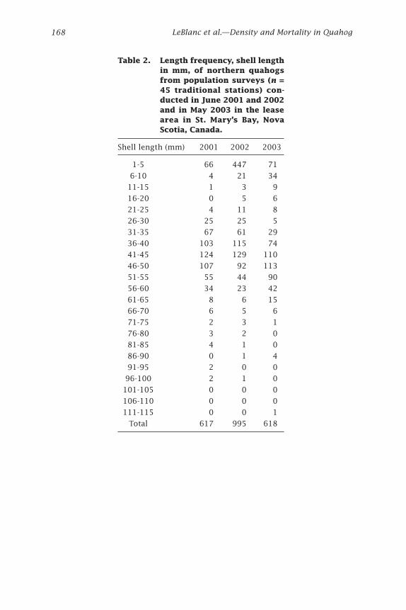
Table 2. Length frequency, shell length in mm, of northern quahogs from population surveys (n = 45 traditional stations) con-ducted in June 2001 and 2002 and in May 2003 in the lease area in St. Mary’s Bay, Nova Scotia, Canada.

Shell length (mm) 2001 2002 2003

1-5 66 447 71

6-10 4 21 34

11-15 1 3 9

16-20 0 5 6

21-25 4 11 8

26-30 25 25 5

31-35 67 61 29

36-40 103 115 74

41-45 124 129 110

46-50 107 92 113

51-55 55 44 90

56-60 34 23 42

61-65 8 6 15

66-70 6 5 6

71-75 2 3 1

76-80 3 2 0

81-85 4 1 0

86-90 0 1 4

91-95 2 0 0

96-100 2 1 0

101-105 0 0 0

106-110 0 0 0

111-115 0 0 1

Total 617 995 618


Table 3. Age composition of quahogs of 25 mm and larger from popula-tion surveys (numbers expanded to the survey area) conducted in June 2001 and 2002 and May 2003 and from the 2003 com-mercial landings in the lease area in St. Mary’s Bay, Nova Scotia, Canada.

Population surveys (thousands) Landings (thousands)

Age 2001 2002 2003 2003

3 2,425 2,039 1,996 0.1

4 4,369 3,949 1,955 0.2

5 22,119 24,061 12,392 19.2

6 59,755 56,786 52,854 692.8

7 107,617 101,312 104,149 1,965.2

8 46,912 44,341 46,625 807.9

9 4,523 3,256 5,442 206.5

10 2,061 3,178 1,861 110.5

11 0 0 0 0.0

12 472 1,417 630 43.4

13 472 472 157 8.0

14 0 0 0 0.0

15 0 472 0 10.1

Unspecifi ed 6,138 472 3,305 344.8

Total 256,865 241,755 231,367 4,208.6

The unspecifi ed group is composed of large individuals, >70 mm and equal to 11 years, for which no age assignment could be made.

The fi shery appears to be exploiting quahogs of 6 years and older. Mean age to market for these quahogs was 7 years and ranged from 5 to 8 years. Populations in the Gulf of St. Lawrence reach commercial market size, shell length 50 mm, between 9 and 13 years (Landry et al. 1993) while southern populations reach market size in 2-5 years (Grizzle et al. 2001). In St. Mary’s Bay, age to market appears to be faster than for populations of the Gulf of St. Lawrence. Diff erences in growth could be attributed to many factors including temperature, food quality and quantity, and salinity.

It is important to note that the age-length key for 2002 was used to calculate the age composition of the 2001-2003 surveys, as well as the commercial harvest in 2003 (Tables 2 and 3). This assumes that during this short period there have not been large changes in growth. The survey age-length key used for the calculations contained few large individuals,


Figure 3. Age composition of quahogs from the 2001-2003 spring surveys (top), and commercial harvest of 2003 (bottom) from the lease in St. Mary’s Bay, Nova Scotia, Canada.

which might have aff ected the estimation of the age composition of com-mercial harvest in 2003. However, for age groups used in the analyses (7-10 years) the age composition was based on 232 readings. There is usually little diffi culty in identifying annuli for these age classes (Jones et al. 1990).

The increasing number of age 3-7 quahogs in the spring surveys for the three years of observations suggested that younger quahogs have a distribution that is larger than the survey area and that quahogs progres-sively “recruit” to the survey area. For St. Mary’s Bay, passive transport may signifi cantly aff ect the distribution of this population, particularly


Figure 4. Catch curves for quahogs in St. Mary’s Bay from the 2001-2003 spring survey age compositions. Closed circles are data points used in the analysis; open circles were not.


Figure 5. Catch curves for quahogs in St. Mary’s Bay from 2003 age composition of commercial harvest. Closed circles are data points used in the analysis; open circles were not.

Figure 6. Combined catch curve analysis of survey numbers along cohorts. Ages 7-10 were used in the analysis. Symbols indicate year classes.


the younger and smaller animals. The movement of smaller quahogs may be caused by storm surges in the 7 m tidal range, which are characteristic to the area. Geospatial diff erences in distribution between spat, juveniles, and adults may have ecological implications to overall population fi tness (Rice et al. 1989). Large concentrations of adult quahogs may also aff ect the recruitment of juvenile quahogs (Rice et al. 1989). Fegley (2001) has also documented that when there are large numbers of widely dispersed spawning quahogs, this can lead to lower fertilization rates.

All of the catch curve analyses of mortality rates suggested that total mortality for ages 7-10 was high. This would include both natural mortal-ity, such as predation and disease, and the commercial harvest.

These estimates assume that the adult portion of the population is closed and thus not subject to emigration or immigration. Because there are no other known adult populations nearby, passive transport such as that hypothesized for small quahogs is considered less likely for the larger adult animals. The analyses conducted on the age-structured data from the surveys for individual years, or the 2003 harvest, also assumed constant recruitment. Survey data from 2001 to 2003 indicated that there was signifi cant variation in recruitment in the area for year classes produced in the early 2000s. However, the analysis of covariance, which used all three years of survey data, showed that there was no signifi cant diff erence in year-class strength for year classes produced in the early to mid-1990s (ages 7-10 in 2001-2003). This analysis, which took into account potential diff erences in year-class strength, also produced a similarly high estimate of total mortality. In summary, all estimates of Z, either from the survey or the harvest data and using various methods, were relatively high. We could not identify specifi c reasons to discount these estimates.

Given the apparent high total mortality, the low estimates of exploi-tation rate for 2003 and of the fraction of the fi shable biomass taken by the fi shery in 2001-2003 would imply that natural mortality on these age groups was unusually high.

Mortality rates for adult quahog populations from New England states are usually low and uniform throughout the year and rarely exceed 50% for age classes between 6 and 10 years (Kennish 1978). Predation may partly explain high mortality rates. Predation by seagulls is common over the lease area. Annual predation rates of seagulls on adult quahogs in the intertidal mudfl at at Hamble Spit in Southampton, England, were estimated at 5-10 individuals per m2 (Hibbert 1977). Large losses of adult quahogs may also be attributed to winterkill caused by ice scour-ing on the lease. Photographs taken of the lease area in December 2002 showed the presence of large ice cakes of 1.5 × 2 × 2 m (height × length × width). Ice cakes covered the intertidal region from January to April 2002-2004. Winterkill has been suggested for losses of large amounts of oysters (Crassostrea virginica) and quahogs throughout much of the


Gulf of St. Lawrence region in 2002-2003 (T. Landry, DFO, pers. comm. 2003). This phenomenon has not been quantifi ed in Atlantic Canada but may be an important factor in the population dynamics of quahogs in St. Mary’s Bay.

Low survival rates can have serious implications for the sustainability of a population. Size structure is important for the reproductive fi tness of a population and in terms of fi shery management. M. mercenaria is described as a protandrous consecutive hermaphrodite, meaning that males typically dominate the younger size classes, the sex ratio changes with age distribution, and the sex ratio of adults is not 1:1 with growth whereby males may still outnumber the females (Eversole 2001). Though separate sexes do exist, fully functional hermaphrodites are common to quahogs (Eversole 2001). In the Gulf of St. Lawrence, sexual maturity can be attained at 25 mm and 30 mm shell lengths for males and females re-spectively with one major spawning event usually occurring in mid-June (Landry et al. 1999). In this case, the fi shery mainly harvests animals that are 45 mm and larger and the bulk of the mortality for quahogs 7 years and older appears to be largely due to causes other than exploitation. If further analyses confi rm these results, this could be a natural character-istic of this population.

In conclusion, while the simple methods used are subject to a num-ber of assumptions that need to be verifi ed, these analyses provide a description of population structure and initial estimates of mortality for this understudied population. In our study, the limited data precluded the use of more complex models but the results underline the usefulness of basic methods to generate hypotheses about population dynamics, in this case high natural mortality. We hope that this information combined with continued sampling of the population and the fi shery will lead to the use of age-structured population models, such as virtual population and statistical catch-at-age analyses, to gain a better understanding of population dynamics of quahogs in St. Mary’s Bay.

AcknowledgmentsThe authors thank Rachel Caissie, André Drapeau, Rémi Sonier, Denise Muise, Keenan Melanson, Scott Bertram, and Jean-François Mallet. Funding for this four-year joint project was provided by the Aquaculture Collab-orative Research and Development Program of DFO. Additional in-kind support for this project was received from IFP.

ReferencesCastagna, M. 1984. Methods of growing Mercenaria mercenaria from post-larval to

preferred-size speed for fi le planting. Aquaculture 39:355-359.


Dillon Jr., R.T., and J.J. Manzi. 1992. Population genetics of the hard clam, Merce-naria mercenaria, at the northern limit of its range. Can. J. Fish. Aquat. Sci. 49:2574-2578.

Eversole, A.G. 2001. Reproduction in Mercenaria mercenaria. In: J.N. Kraeuter and M. Castagna (eds.), Biology of the hard clam. Elsevier, New York, pp. 221-260.

Fegley, S.R. 2001. Demography and dynamics of hard clam populations. In: J.N. Kraeuter and M. Castagna (eds.), Biology of the hard clam. Elsevier, New York, pp. 383-422.

Grizzle, R.E., V.M. Bricelj, and S.E. Shumway. 2001. Physiological ecology of Merce-naria mercenaria. In: J.N. Kraeuter and M. Castagna (eds.), Biology of the hard clam. Elsevier, New York, pp. 305-382.

Hibbert, C.J. 1977. Growth and survivorship in a tidal-fl at population of the bivalve Mercenaria mercenaria from Southampton water. Mar. Biol. 44:71-76.

Hilborn, R., and C.J. Walters. 1992. Quantitative fi sheries stock assessment: Choice, dynamics and uncertainty. Chapman and Hall, New York. 570 pp.

Jones, D.S., I.R. Quitmyer, W.S. Arnold, and D.C. Marelli. 1990. Annual shell banding, age and growth rate of hard clams (Mercenaria spp.) from Florida. J. Shellfi sh Res. 9(1):215-225.

Kennish, M.J. 1978. Eff ects of thermal discharges on mortality of Mercenaria mer-cenaria in Barnegat Bay, New Jersey. Environ. Geol. 2:223-254.

Landry, T., and T.W. Sephton. 1996. Southern Gulf northern quahaug. DFO Atlantic Fisheries Stock Status Report 96/102E. 3 pp.

Landry, T., T.W. Sephton, and D.A. Jones. 1993. Growth and mortality of northern quahaug Mercenaria mercenaria (Linnaeus, 1758), in Prince Edward Island. J. Shellfi sh Res. 12(2):321-327.

Landry, T., M. Hardy, M. Ouellette, N.G. MacNair, and A. Boghen. 1999. Reproductive biology of the northern quahaug, Mercenaria mercenaria, in Prince Edward Island. Can. Tech. Rep. Fish. Aquat. Sci. 2287. 18 pp.

Rice, M.A., C. Hickox, and I. Zehra 1989. Eff ects of intensive fi shing eff ort on the population structure of quahogs, Mercenaria mercenaria (Linnaeus 1758), in Narragansett Bay. J. Shellfi sh Res. 8(2):345-354.

Ricker, W.E. 1975. Computation and interpretation of biological statistics of fi sh populations. Bull. Fish. Res. Board Can. 191. 382 pp.

Ropes, J.W., and L. O’Brien. 1979. A unique method of aging surf clams. Bull. Am. Malacol. Union Inc. 1978:58-61.

Sephton, T.W., and C.F. Bryan. 1990. Age and growth rate determinations for the Atlantic surf clam, Spisula solidissima (Dillwyn, 1817), in Prince Edward Island, Can. J. Shellfi sh Res. 9(1):177-185.

Sinclair, A.F. 2001. Natural mortality of cod (Gadus morhua) in the southern Gulf of St. Lawrence. ICES J. Mar. Sci. 58:1-10.

Whiteaves, J.F. 1901. Catalogue of the marine invertebrates of eastern Canada. S.E. Dawson, Ottawa, Ontario. 271 pp.


177

Timing of Parturition and Management of Spiny Dogfi sh in WashingtonCindy A. TribuzioUniversity of Alaska Fairbanks, School of Fisheries and Ocean Sciences, Juneau, Alaska, and University of Washington, School of Aquatic and Fishery Sciences, Seattle, Washington

Vincent F. GallucciUniversity of Washington, School of Aquatic and Fishery Sciences, Seattle, Washington

Greg BargmannWashington State Department of Fish and Wildlife, Olympia, Washington

AbstractManagement of the spiny dogfi sh (Squalus acanthias) fi shery in the east-ern North Pacifi c Ocean has historically been limited, and not focused on conservation of the species. Washington State Department of Fish and Wildlife (WDFW) recently adopted a new management strategy aimed spe-cifi cally at protecting the spiny dogfi sh during the critical reproductive period. There is currently little information on the reproductive biology of the Puget Sound stocks of spiny dogfi sh, and much of it is anecdotal. The aim of this project is to improve the data poor nature of spiny dog-fi sh fi shery management. This paper reports some of the fi ndings of an extensive investigation into the reproductive biology of Puget Sound spiny dogfi sh. The pupping season appears to be from May through No-vember, longer than the anecdotal data indicate and much longer than current regulations were written to cover.

IntroductionThe spiny dogfi sh (Squalus acanthias) fi shery in the Puget Sound and Pacifi c Northwest waters has received little management and has been

Tribuzio et al.—Parturition and Management of Spiny Dogfi sh178

characterized by fl uctuations in catch and eff ort. Management of this species in Puget Sound is based on poor data, managers have little local information about the species, and much of that information is anecdotal and from fi shery stakeholders. Prior to 2003, spiny dogfi sh management goals were reduction of interactions with other fi sheries, reduction of bycatch, or to conform to market practices (WDFW 2003).

In 2003, Washington Department of Fish and Wildlife (WDFW) amend-ed the fi shing regulations for setnet and set-line spiny dogfi sh fi sher-ies. The 2003 amendments eff ectively closed the fi shery in most of the Puget Sound areas during the summer months (June 16–September 15). This time frame was suggested by industry as the period when females were pupping and was adopted into the regulation. The impetus to put regulations in place was justifi ed by the generally accepted need to prac-tice precautionary management (FAO 1995) to conserve the species and maintain the fi shery.

Recent stock assessments in the western North Atlantic have shown that the stocks are not stable, fi shable biomass has greatly decreased, there is low recruitment of females, and the stocks may be fully exploited (Rago et al. 1998). Managers took dramatic steps to reduce the impact on the stocks as a whole and on large females in particular. While stocks have not had the same trend in Washington state waters, there is cause for concern. Catch rates have shown dramatic declines over the last two decades (Fig. 1) and recent stock assessments also suggest a decline (WDFW 2003). In neighboring British Columbia, stock assessments show their stocks to be stable. Given the geographic range of the stocks in the eastern North Pacifi c (WDFW 2003, McFarlane and King 2003), the popula-tions are transboundary and require cooperative management between the two countries. This begins with creating accurate methods for assess-ing the status of these stocks, and managing accordingly.

Squalus acanthias is common, small, and easy to maintain in labora-tory conditions. Literature on this species comes from many areas: North Atlantic (Rago et al 1998, Soldat 2002), North Sea (Stenberg 2002, Jones and Ugland 2001), Black Sea (Polat and Guemes 1995), and the North Pacifi c (Bonham 1954; Holland 1957; Ketchen 1972, 1975, 1986; Wood et al. 1979; McFarlane and Beamish 1987; Saunders and McFarlane 1993; McFarlane and King 2003). Laboratory studies with detailed examina-tions of the anatomy, physiology, and reproductive cycles, including endocrinology have been conducted (Tsang and Callard 1987, Koob and Callard 1999).

In 1948, Bigelow and Schroeder determined that the populations in the North Pacifi c were the same species as those in the North Atlantic. However, research indicates that the animals in these two areas do diff er in some aspects. In the North Pacifi c, the spiny dogfi sh are longer lived, mature later and at a larger size, and they grow much larger than those


in the North Atlantic (Ketchen 1972, 1975; McFarlane and Beamish 1987; Saunders and McFarlane 1993).

In the eastern Pacifi c Ocean, spiny dogfi sh research has focused on aging, migrations, and population dynamics (Bonham 1954, Holland 1957, Wood et al. 1979, McFarlane and Beamish 1987, Saunders and McFarlane 1993, McFarlane and King 2003) with less emphasis on life history. McFarlane and King (2003) show some animals move between Strait of Georgia and Puget Sound waters, and that the animals from the coastal tagging area (west coast Vancouver Island) are more prone to migration. Three separate stocks have been identifi ed by McFarlane and King (2003) and WDFW (2003): coastal stocks (including Washington coast, and west coast Vancouver Island), northern (including the Strait of Georgia and the San Juan archipelago) and southern (waters from Port Townsend to the south).

Around the world, pupping and mating seasons vary by area. An in-depth analysis of reproductive biology for spiny dogfi sh found in British Columbia waters suggested that mating occurs from December through February and that parturition occurs October through November (Ketchen 1972). Soldat (2002) reported that pupping in the western North Atlantic

0

500

1000

1500

2000

2500

3000

3500

4000

4500

1965 1970 1975 1980 1985 1990 1995 2000 2005

Year

Co

mm

erci

al C

atch

(t)

Figure 1. Commercial landings in metric tons for Puget Sound spiny dog-fi sh.


occurs year-round with most activity between November and April. In waters near Sweden and Norway, pupping is reported to occur from No-vember to December and mating from December to February (Stenberg 2002), while Jones and Ugland (2001) report pupping from September to December and fertilization (and onset of pregnancy) from October to February. It is important to note that the time of mating and the onset of pregnancy may not be closely linked if the female stores the sperm for a period of time prior to fertilization. The objective of this paper is to present results from an ongoing and in-depth study into the reproductive biology of spiny dogfi sh in Puget Sound. We propose that the timing of the critical reproductive events may diff er from that previously reported, which has a direct impact on current management strategies.

Our investigation of the reproductive biology of the spiny dogfi sh is an eff ort to refi ne parameters for more accurate stock assessment and management strategies. Although this study focuses on the spiny dogfi sh in north Puget Sound (NPS), we also sampled spiny dogfi sh from the south Puget Sound (SPS), east Puget Sound (EPS), and coastal (C) areas, in an ef-fort to compare reproductive timing and animal sizes (Fig. 2). The results presented in this paper will quantify the reproductive season for NPS spiny dogfi sh, contribute to a comparison of the timing of reproductive seasons with spiny dogfi sh from other areas, and suggest the role of this information in defi ning fi shing seasons and harvest regulations. Informa-tion from this study will contribute to management of the spiny dogfi sh fi shery in Puget Sound, and possibly to British Columbia management.

Materials and methodsThis study has three parts: sample collection, lab analysis, and hormone analysis. Sample collections involved demographic information, size and sex distributions, and catch eff ort. The laboratory section included examination and measurement of reproductive tracts. The hormone component is not presented here but will appear in a future paper (M.S. thesis draft, Cindy A. Tribuzio).

Spiny dogfi sh samples were collected from November 2002 to Octo-ber 2003. Fish were sampled from the catch of a commercial bottom trawl fi sherman in the southern Strait of Georgia, Washington (48ºN, 123ºW) between 73 and 128 meters (40-70 fathoms) depth (Fig. 2). Up to 25 spiny dogfi sh were taken from the trawl catch on each sampling date and main-tained in an onboard live tank with fl owing seawater until brought to the dock. This was not considered a random subsample, as the vagaries of the collection eff ort did not allow for guarantee of randomization. Non-ran-dom samples may induce size bias, and while the captain was instructed to randomly sub-sample animals, it is the nature of the fi shery to take the largest, and it is possible that our samples are upwardly biased. Given the nature of the project objectives, the non-random sampling and possible


Figure 2. Map of fi shing areas for this study. NPS = north Puget Sound, EPS = east Puget Sound, SPS = south Puget Sound, and C = coastal.

bias are inconsequential. Fish were processed at the Sea-K Warehouse in Blaine, Washington. Dockside processing allowed WDFW samplers to col-lect the data from fresh fi sh without requiring samplers to be onboard the vessel and without requiring samples to be frozen.

Each animal was weighed whole and data recorded for pre-caudal length (PCL), fork length (FL), and total length-natural (TLnat) (Fig. 3). To compare length distributions to previous studies 146 spiny dogfi sh were randomly sampled from the same fi shing ground and measured for TLnat and TLext (Fig. 3). Male clasper inner length (CIL) was also measured. Blood

125 W 124 W 123 W 122 W

46 N

47

N

48

N

49 N


was collected (~5ml), in a 15 ml centrifuge tube, from the caudal vein by removing the caudal fi n and catching the blood fl owing from vein. These tubes were kept cold overnight to allow the blood to clot and the serum to separate out. The serum was drawn from each blood sample and divided into 3 separate 1.5 ml micro-centrifuge tubes, prior to shipping. Samples were kept on ice, not frozen, and shipped overnight to the University of Washington for further analysis.

The second dorsal spine was removed, from tip to vertebrae, for age determination. Maturity stages of the reproductive tracts (based on Stehmann 2002) were recorded, and the entire female reproductive tract or testes (males) were removed and kept on ice.

Female reproductive tracts were measured for length, width (both to the nearest millimeter) and weight (to the nearest tenth of a gram) of ovaries, oviducts, oviducal glands, and uteri. In adult females (Stehm-ann 2002, stages D-G), the diameters of the developing ova within the ovary were measured to the nearest millimeter. In pregnant females with

Figure 3. Length measurements for whole animal. Lower left, tail in natural position for measuring TLnat. Lower right, tail extended to line up with body, for measuring TLext.


candles, the candles were weighed and the number of eggs counted. For those females with pups, each pup was weighed with and without the yolk sac, sexed, and measured for PCL, FL, and TLext. For male spiny dog-fi sh, the testes were weighed and measured for length and width.

Maturity classifi cations in the fi eld were based on Stehmann (2003). However, the reproductive analysis in this project required a fi ne scale. We initially used a scale proposed by Tsang and Callard (1987), with 4 reproductive stages and did not account for post-natal females (Table 1). Table 1 shows the stages used for this study. The stages of pregnancy were based on the presence of candles with embryos too small to measure with the naked eye, those with embryos in candles that were measurable, and those females with embryos free of the candle in the uterus based on size. Given the extended gestation in this species and the short period between pregnancies we classifi ed all mature females with empty uteri as spent/post-natal or pre-fertilization (stage I).

Samples from outside the above sample area were also collected for comparison during the summer of 2003 (Fig. 2). For comparison, spiny dogfi sh from Willapa Bay, Washington (C) and south Puget Sound (SPS) were collected as bycatch in ongoing research by WDFW. Targeted hook and line fi shing for spiny dogfi sh was conducted near Orcas Island, Wash-ington (EPS). For most of these samples the only measurements taken

Table 1. Comparison of pregnancy stages from a previous study and this study.

Tsang and Callard 1987 This study

Stage Description Stage Description

A Candles, embryos up to 3.5 cm, follicles 3�10 mm

A Candle present, embryo not measurable

B Embryos 3�10 cm, follicles 17�20 mm

B Candle present, embryo measurable

C Embryos 17�25 cm, follicles 28�34 mm

C No candle, embryo TL < 10 cm

D Embryos >25 cm, follicles 32�38 mm

D Embryo TL 10.1�15 cm

E Embryo TL 15.1�17.5 cm

F Embryo TL 17.6�20.5 cm

G1 Embryo TL 20.6�23 cm

G2 Embryo TL 22.5�24.5 cm

H No external yolk sac embryo TL 10.1�15 cm

I Post�partum

TL = total length.


were sex, lengths, weight, maturity, and blood, while a few were sent to the lab for further measurements.

ResultsThis paper reports on results from the fi rst 11 months of a 12-month sam-pling program. Sampling catch rates were relatively constant throughout the sampling period, with the exception of early spring and early summer (Fig. 4). The sampling plan was for two trips each month, approximately every other week, with a targeted sample number of 25 fi sh for each trip. Due to weather (wind and tides) fi shing did not always occur regularly. Inclement windy weather was the primary factor contributing to the low fi shing eff ort during the period 26 February 2003 and 14 April 2003, resulting in no samples in March. Fishing was not aff ected by weather during the period from 14 May 2003 to 11 June 2003, but catches of spiny dogfi sh were lower during that period.

Numbers and maturities of males and females varied between sam-pling dates. Mature males were caught consistently from 7 November 2002 to 27 February 2003 (Fig. 5). Between 27 February 2003 and 29

*

0

5

10

15

20

25

7-Nov

-02

14-N

ov-0

2

25-N

ov-0

2

5-Dec

-02

7-Ja

n-03

27-J

an-0

3

10-F

eb-0

3

26-F

eb-0

3

27-F

eb-0

3

Mar

ch r

14-A

p-0

3

22-A

pr-0

3

Average

29-A

pr-0

3

8-M

ay-0

3

14-M

ay-0

3

27-M

ay-0

3

11-J

un-0

3

17-J

ul-03

29-J

ul-03

11-A

ug-0

3

26-A

ug-0

3

9-Sep

-03

17-S

ep-0

3

2-Oct-

03

6-Oct-

03

Sampling Date

Sam

ple

Siz

e

males females

Figure 4. Total catch for each sampling date. Star (*) represents when no sampling occurred. N = 471.


April 2003, the maturity of the males sampled changed signifi cantly, with immature animals becoming prominent (t-test, alpha = 0.05, P-value = 0.002). In the early summer months (May and June) mature males become more prominent in the catch and peaked at 26 Aug 2003. The composition of the female catch varied more than the males throughout the sampling period (Fig. 6). Immature females made up most of the fe-male catch 7 November 2002 to 5 December 2002, 26 February 2003 to 14 May 2003, 11 June 2003, and 29 July 2003 to 9 September 2003. At no point was the female catch composed entirely of mature animals, but between 26 February 2003 and 14 May 2003, and between 29 July 2003 and 9 September 2003, there was a signifi cant increase in the proportion of immature females sampled (t-test, alpha = 0.05, P-value < 0.001).

Reproductive seasonalityThe relative frequency of mature females in each stage for each month sampled shows that post-natal females (stage I, Fig. 7) were present much of the year, but were absent most of February (after 10 February 2003,

Males 9610 81 4 11 14 8 5 5 9 712 4 10 3 15 21 7 1

* 0000

0.1

0.2

0.3

0.4

0.5

0.6

0.7

0.8

0.9

1

Pro

po

rtio

n o

f S

amp

lemature immature

7-Nov

-02

14-N

ov-0

2

25-N

ov-0

2

5-Dec

-02

7-Ja

n-03

27-J

an-0

3

10-F

eb-0

3

26-F

eb-0

3

27-F

eb-0

3

Mar

ch

14-A

pr-0

3

22-A

pr-0

3

29-A

pr-0

3

8-M

ay-0

3

14-M

ay-0

3

27-M

ay-0

3

11-J

un-0

3

17-J

ul-03

29-J

ul-03

11-A

ug-0

3

26-A

ug-0

3

9-Sep

-03

17-S

ep-0

3

2-Oct-

03

6-Oct-

03

Sampling Date

Figure 5. Male catches by month for mature and immature animals. Star (*) represents when no sampling occurred, numbers above the bars represent sample size. N = 170.


only two mature females were sampled) and April (one mature female was sampled during the last sampling event in April; no samples were collected in March). However, this was also the time of least intensive sampling. Stage I females were caught with the greatest frequency (the entire mature female catch) in June and September, and made up a large portion of the mature female catch in July and August. Late stage preg-nancy females (stages G and H) were also present in July and August. The least frequent catches of stages, G-H, were in January through May, where the earlier stages of pregnancy were seen most often (stages A-B). Females may begin pupping in June and continue through November, while ovula-tion and fertilization occur November through February.

With the gestation occurring over about 22 months, in the popula-tion there are two groups of pregnant females: those in the fi rst year of pregnancy and those in the second year. The graph of embryo size against sampling date shows this trend (Fig. 8). There were no females caught that were in the fi rst year of pregnancy, in the months of August and September (in September, all females were stage I). In November and December 2002 and October 2003, embryos of three stages are seen

Females2

*

1 19 16 24 17 21 14 11 5 1610 13 4 10 15 25 22 10 184 25 7 24

0

0.1

0.2

0.3

0.4

0.5

0.6

0.7

0.8

0.9

1

7-Nov

-02

14-N

ov-0

2

25-N

ov-0

2

5-Dec

-02

7-Ja

n-03

27-J

an-0

3

10-F

eb-0

3

26-F

eb-0

3

27-F

eb-0

3

Mar

ch

14-A

pr-0

3

22-A

pr-0

3

29-A

pr-0

3

8-M

ay-0

3

14-M

ay-0

3

27-M

ay-0

3

11-J

un-0

3

17-J

ul-03

29-J

ul-03

11-A

ug-0

3

26-A

ug-0

3

9-Sep

-03

17-S

ep-0

3

2-Oct-

03

6-Oct-

03

Sampling Date

Pro

po

rtio

n o

f S

amp

le

mature immature

Figure 6. Female catches by month for mature and immature animals. Star (*) represents when no sampling occurred, numbers above the bars represent sample size. N = 333.


1 431832818

*

13241517

0%

10%

20%

30%

40%

50%

60%

70%

80%

90%

100%

Nov Dec Jan Feb Mar Apr May Jun Jul Aug Sept Oct

Fem

ales

IHG2G1FEDCBA

Figure 7. Frequency of pregnancy stages for mature females. Stage A rep-resents the earliest stages of pregnancy through stage I which represents spent females. N = 171.

simultaneously, indicating some temporal overlap between pupping and fertilization.

Comparisons to other areasThree areas sampled around Puget Sound and coastal Washington state waters were compared for diff erences in size and stage of maturity. For females all three areas were sampled in July and August, and just the north Puget Sound (NPS) and coastal (C) areas in September. In July, the sizes of the females caught were signifi cantly diff erent in the three areas (t-test, alpha = 0.05, all P-values < 0.004), but in August and September, the sizes were not signifi cantly diff erent from one another (t-test, alpha = 0.05, all P-values > 0.166). Males were encountered only in NPS and C and only in July and August. As with females, the sizes were signifi cantly diff erent between the two areas in July (t-test, alpha = 0.05, P-value = 0.01) but not in August (t-test, alpha = 0.05, P-value = 0.105). Also, tests between months within the same area showed that in NPS and C, diff erent sized females were caught in July than in August (t-test, alpha = 0.05, P-values < 0.001), and between August and September in NPS (t-test, alpha


= 0.05, P-value < 0.01). Coastal males caught in July and August were also signifi cantly diff erent in size (t-test, alpha = 0.05, P-value < 0.01).

The relative frequencies of females in each stage of the reproduc-tive cycle were compared for the females in all three areas in the month of July (Fig. 9). A Mann-Whitney U test for ordinal data was used to test the null hypothesis that the regions have the same reproductive stage frequencies and thus the same timing of reproductive events. The null hypothesis was rejected for all three tests conducted (alpha = 0.05, all P-values < 0.001), and the three regions were all signifi cantly diff erent from each other in the frequencies of females in reproductive stages.

DiscussionThe principal consideration in the WDFW 2003 management plan was timing of parturition. The NPS samples indicate that there may be a pro-longed pupping season, which contrasts with earlier studies in nearby areas. Ketchen (1972) reported that pupping in British Columbia occurs in October and November and breeding December through February. At

0

50

100

150

200

250

300

Nov-02 Dec-02 Jan-03 Feb-03 Mar-03 Apr-03 May-03 Jun-03 Jul-03 Aug-03 Sep-03 Oct-03

Timeline

TL

(m

m)

Figure 8. Embryo lengths by catch date. At least two distinct size classes are seen throughout the time frame of sampling. Zero values represent embryos that are still in the candle stage and are not measurable to the naked eye. N = 370.


public aquariums in the Pacifi c Northwest, spiny dogfi sh show diff erent reproductive timing. Pups have been found in December and January at the Seattle Aquarium, and records at the Point Defi ance Zoo and Aquari-um show pupping roughly March through June (Jeff Christiansen, Seattle Aquarium, pers. comm., September 2003; John Rupp, Point Defi ance Zoo and Aquarium, Tacoma, pers. comm., September 2003). The animals on display at both aquariums were from stocks in Puget Sound. The Oregon Coast Aquarium, with spiny dogfi sh from coastal stocks near Newport, Oregon, reports pupping for all months except March, July, August, and November with peaks in May and October. Evidence of mating (damage to caudal and pectoral fi ns from biting males) has been recorded in March, June, July, and September (Colleen Green, Oregon Coast Aquarium, New-port, pers. comm., September 2003). Evidence of mating, however, is not necessarily indicative of fertilization and pregnancy; there may be a time lag due to the possibility of storage of sperm in the oviducal gland for a signifi cant period of time. This phenomenon has not been studied in spiny dogfi sh.

N=28 N=8 N=22

0

0.1

0.2

0.3

0.4

0.5

0.6

0.7

NPS SPS C

Region

Rel

ativ

e F

req

uen

cy

DEFG

Figure 9. Comparison of uterine (pregnancy) stages in three diff erent sampling areas. D = early pregnancy, E = mid pregnancy, F = late, and G = post partum (Stehmann 2002). NPS = north Puget Sound, SPS = south Puget Sound, C = coastal.


Our study suggests that pupping occurs from May to November for the NPS stocks and ovulation and fertilization from October to January. It is also possible that the spiny dogfi sh exhibit a year-round reproductive seasonality with peaks in activity. Data on reproductive females were lacking between much of February through late April, and more intense sampling during that period may provide more insight into the seasonal pattern. Most reports for spiny dogfi sh are that they have either a specifi c seasonality or a prolonged seasonality to their reproductive cycle.

Females in the earliest stages of pregnancy (stage A: eggs are still contained within the candles in utero and the embryos are too small to be measured with the naked eye) were encountered from November through February. Jones and Ugland (2001) estimated the candle stage to last 13 months and Ketchen (1972) estimated length of embryos at the end of the fi rst year to be about 14-15 cm. In this study, we consider the candle stage in two parts (Table 1): one where the embryo cannot be measured and the other where it can be measured by the naked eye. We estimate that the candle stage lasts less than one year and that stage A lasts about 1 month. The average monthly growth rate estimate for the fi rst year is 11.67-12.50 mm (assuming that growth is constant during that year), based on Ketchen (1972). The smallest embryo we found not contained in a candle was 71 mm TLext and the largest within a candle was 49 mm TLext. Based on these observations and the proposed growth rate, the en-tire candle stage lasts somewhere between 3.9 months and 6.1 months. The smallest measurable embryos still in the candle were about 12.5 mm, which takes an estimated 1-1.07 months to achieve. We can assume that females in stage A of pregnancy have been pregnant for only about 1 month, thus those females encountered in stage A during November may have ovulated and fertilized in October, and those encountered in February became pregnant in January. Since samples were not taken in March, we were unable to determine if this period extends through Febru-ary. No stage A females were encountered in April, indicating ovulation and fertilization were completed by March.

With the gestation being about 22 months long, the ovaries must continuously develop the next cohort of eggs instead of having a resting period between pregnancies. The next crop of eggs is then developing for the subsequent pregnancy while the current pregnancy is ongoing. After the female has pupped, the eggs fi nish development, ovulate, are fertilized, and move to the uteri. Maximum ova diameters are seen in September and November (prior to the fi nal sampling event in October), and again in February. Given the broad temporal span of the pupping season, the measurements of ova diameter from spent females would be expected to vary over the time period. However, the variation in the size through time appears to fall into two groups of development, suggesting two broad and overlapping pupping seasons; the fi rst being in the early summer and the next in the fall.


As with the developing ova, the developing embryos can be used to support the timing of reproductive events. Data for embryonic growth show two distinct groups of development, which are explained by the almost two-year gestation. Pregnant, mature females are either in their fi rst or second year of gestation. Currently there is no evidence to suggest that females segregate by year of gestation. However, within these two-year classes of gestation, there does appear to be variation in the degree of embryo development, suggesting more broad timing of fertilization (Fig. 8).

Spiny dogfi sh harvest encompasses areas outside the NPS, so manage-ment strategies will need to be fl exible enough to encompass the timing of reproductive events in the various areas. Comparisons between fi sh-ing areas in south Puget Sound (SPS) and coastal (C) waters were made. These comparisons did suggest diff erences in the timing of reproductive events in the three areas during the month of July. This relationship will be examined further in future reports.

This study was undertaken to investigate the timing of critical repro-ductive events to assist with development of management. The current management plan closes the fi shery during the time period perceived to be when the females are most vulnerable. This paper is the fi rst in a series that examines these events as well as reproductive physiology, endocri-nology, and embryonic development. This paper specifi cally reports on the timing of pupping and fertilization, which is more broad than expect-ed. The pupping season appears to extend well past the time frame over which WDFW enacted fi shing closures, and is diff erent from published data on nearby British Columbia populations. The data presented are for a one-year period. We have no evidence that year-to-year variability is minimal, so that the 2002-2003 data may not be representative. We sug-gest extending this study and refi ning the methods based on what was learned during this fi rst year if more precise dates are needed.

AcknowledgmentsWe thank Washington State Department of Fish and Wildlife for support-ing this project with funding and valuable staff hours. Sue Hoff mann and Debbie Farrer at WDFW worked countless hours and late nights dissecting out reproductive tracts, for which we are very grateful. Heather Weinden-hoft and Danny Badger helped with sample collection and lab analysis. Shawn Waters, skipper of the F/V Tulip, supplied time and eff ort in catch-ing and maintaining the spiny dogfi sh onboard his boat. Sea-K Fisheries allowed us to use warehouse space and accommodated our sampling needs. We also thank the students in the University of Washington School of Aquatic and Fishery Sciences shark group, who helped with advice, ideas, input, and sampling.


ReferencesBigelow, H.B., and W.C. Schroeder. 1948. Lancelets, cyclostomes and sharks. In:

Fishes of the western North Atlantic, Part 1. Memoir. Sears Foundation for Marine Research. 576 pp.

Bonham, K. 1954. Food of the dogfi sh Squalus acanthias. Washington Department of Fisheries, Fisheries Research Papers 1:25-36.

FAO. 1995. Guidelines on the precautionary approach to capture fi sheries and species introductions. FAO Fish. Tech. Pap. 350(Part 1). 52 pp.

Holland, G.A. 1957. Migration and growth of the dogfi sh shark, Squalus acanthias (Linnaeus), of the eastern North Pacifi c. Washington Department of Fisheries, Fisheries Research Papers 2:43-59.

Jones, T.S., and K.I. Ugland. 2001. Reproduction of female spiny dogfi sh, Squalus acanthias, in the Oslofjord. Fish. Bull. U.S. 99:685-690.

Ketchen, K.S. 1972. Size at maturity, fecundity, and embryonic growth of the spiny dogfi sh (Squalus acanthias) in British Columbia waters. J. Fish. Res. Board Can. 29:1717-1723.

Ketchen, K.S. 1975. Age and growth of dogfi sh Squalus acanthias in British Columbia waters. J. Fish. Res. Board Can. 32:43-59.

Ketchen, K.S. 1986. The spiny dogfi sh (Squalus acanthias) in the northeast Pacifi c and a history of its utilization. Can. Spec. Publ. Fish. Aquat. Sci. 88. 78 pp.

Koob, T.J., and I.P. Callard. 1999. Reproductive endocrinology of female elas-mobranchs: Lessons from the little skate (Raja erinacea) and spiny dogfi sh (Squalus acanthias). J. Exp. Zool. 284:557-574.

McFarlane, G.A., and R.J. Beamish. 1987. Validation of the dorsal spine method of age determination for spiny dogfi sh. In: R.C. Summerfelt and G.E. Hall (eds.), The age and growth of fi sh. Iowa State University Press, Ames, pp. 287-300.

McFarlane, G.A., and J.R. King. 2003. Migration patterns of spiny dogfi sh (Squalus acanthias) in the North Pacifi c Ocean. Fish. Bull. U.S. 101:358-367.

Polat, N., and A.K. Guemes. 1995. Age determination of spiny dogfi sh (Squalus acan-thias L. 1758) in Black Sea waters. Isr. J. Aquacult. Bamidgeh 47(1):17-24.

Rago, P.J., K.A. Sosebee, J.K.T. Brodziak, S.A. Murawski, and E.D. Anderson. 1998. Implications of recent increases in catches on the dynamics of northwest Atlantic spiny dogfi sh (Squalus acanthias). Fish. Res. 39:165-181.

Saunders, M.W., and G.A. McFarlane. 1993. Age and length at maturity of the female spiny dogfi sh, Squalus acanthias, in the Strait of Georgia, British Columbia, Canada. In: J.P. Wourms and L.S. Demski (eds.), The reproduction and develop-ment of sharks, skates, rays and ratfi shes. Environ. Biol. Fishes 38:49-57.

Soldat, V.T. 2002. Spiny dogfi sh (Squalus acanthias L.) of the northwest Atlantic Ocean (NWA). Sci. Counc. Res. Doc. NAFO 2(84). 33 pp.

Stehmann, M.F.W. 2002. Proposal of a maturity stages scale for oviparous and viviparous cartilaginous fi shes (Pisces, Chondrichthyes). Arch. Fish. Mar. Res. 50:23-48.


Stenberg, C. 2002. Life history of the piked dogfi sh (Squalus acanthias L.) in Swed-ish waters. Sci. Counc. Res. Doc. NAFO 2(13).

Tsang, P.C.W., and I.P. Callard. 1987. Morphological and endocrine correlates of the reproductive cycle of the aplacental viviparous dogfi sh, Squalus acanthias. Gen. Comp. Endocrin. 66:182-189.

WDFW. 2003. Spiny dogfi sh stocks in Puget Sound: Fisheries and stock status. Washington Department of Fish and Wildlife (WDFW) draft document. Janu-ary 2003. 46 pp.

Wood, C.C., K.S. Ketchen, and R.J. Beamish. 1979. Population dynamics of spiny dogfi sh (Squalus acanthias) in British Columbia waters. J. Fish. Res. Board Can. 36:647-656.


195

Developing Assessments and Performance Indicators for a Small-Scale Temperate Reef Fish FisheryPhilippe E. Ziegler, Jeremy M. Lyle, Malcolm Haddon, and Paul BurchMarine Research Laboratories, Tasmanian Aquaculture and Fisheries Institute (TAFI), University of Tasmania, Tasmania, Australia

Abstract In Australia, the development of live fi sh markets in the early 1990s cre-ated strong demand for temperate reef fi sh species, particularly banded morwong (Cheilodactylus spectabilis). The fi shery expanded rapidly over a very short period but has subsequently undergone a marked decline. Several management controls have been progressively introduced, in-cluding size limits, seasonal closures, and limited entry. Only simple performance indicators based on catch and catch rate trends have been utilized to monitor stocks.

Banded morwong are sedentary and appear to have a depth-struc-tured sex and size distribution. They are long-lived (>80 years), and growth rates and maximum sizes are distinctly diff erent for males and females. These life-history characteristics and the likely population structuring at small spatial scales have marked consequences for stock assessment.

A variety of simple assessment approaches, including catch rate standardization, yield-per-recruit and spawning biomass-per-recruit analyses, catch curve analysis, and biological indicators (median size and age, sex ratio) have been examined. These methods proved inconclusive in indicating whether current fi shing levels are sustainable, or based on continued reduction of accumulated biomass and/or serial depletion of spatially structured populations. General uncertainty regarding data qual-ity from the commercial fi shery and spatial representation of biological data within the populations are of concern.

Ziegler et al.—Small-Scale Reef Fishery196

Because data intensive assessment techniques cannot be justifi ed for this small-scale fi shery, we propose the development of an operating model that can be used to evaluate whether simple biological and/or fi shery indicators can assist performance monitoring and address issues of sustainability.

IntroductionThe development of live-fi sh fi sheries in Australia during the 1990s has placed increased pressure on tropical and temperate reef fi sh popula-tions, with fi sheries expanding rapidly during the mid to late 1990s (Rimmer and Franklin 1997). Recent annual production from the tropical fi sheries has exceeded 1,500 metric tons (QDPI 2002), much of which is exported to Asian markets. By contrast, catches from the temperate fi sheries, principally banded morwong (Cheilodactylus spectabilis) and wrasse (Notolabrus spp.), are low, in the order of 200 t, and service do-mestic live-fi sh markets.

Typically reef fi sh populations are spatially structured and reef fi sh fi sheries tend to be small in size. This combination makes the applica-tion of data intensive assessment techniques diffi cult to justify both practically and economically. Using banded morwong as a case study, we examine the current stock assessment approaches applied in Tasmania, Australia. First, we evaluate catch and eff ort data and then investigate al-ternative assessments and reference points based on available biological information. Industry perceptions about resource status, fi sh behavior, and fi shery developments have also been canvassed to supplement bio-logical and fi shery information. Our data, however, are patchy in space and time and present signifi cant challenges when applied to assessing stock status.

Banded morwong fi sheryThe live-fi sh fi shery for banded morwong is a coastal gillnet fi shery off eastern Tasmania, with catches concentrated off the central and south-east coasts (Fig. 1). The fi shery expanded rapidly in the early 1990s and reported catches peaked at almost 150 t in 1993-1994 (November-October fi shing year, Fig. 2). Between 1994-1995 and 1999-2000, annual produc-tion declined steadily to below 40 t but has since stabilized at around 50 t, with catches generally tracking changes in eff ort.

Fishers generally operate out of dinghies or small vessels and tar-get banded morwong using a fl eet of large mesh gillnets (130-140 mm) over exposed rocky reefs. To minimize eff ects of barotrauma and thus maximize fi sh survival, fi shing is largely restricted to maximum depths of about 25 m even though the species occurs to greater depths.

Despite low production and value, currently less than AU$ 0.7 million per year, the fi shery is highly regulated. Minimum and maximum size lim-


Figure 1. Map of Tasmania indicating total catches of banded morwong by 30 nautical mile fi shing block summed over the period 1995-1996 to 2002-2003.

its (330 and 430 mm fork length, FL) were introduced in 1994 to protect large adults and permit spawning prior to recruitment to the fi shery, in addition to matching market size requirements. In 1998 both limits were increased by 30 mm after it became apparent that they off ered minimal protection to mature females and the lower limit was set close to the size at maturity (Murphy and Lyle 1999). A two-month closed season during the peak spawning period (March and April) was introduced in 1995 and has remained in place since that time. Interim licensing arrangements were implemented in 1996, with around 90 live-fi sh endorsements issued,


and replaced by a specifi c banded morwong license in 1998. There are currently 29 license holders.

Management of the fi shery falls under the Tasmanian Scalefi sh Fish-ery Management Plan (DPIF 1998). The plan contains a series of perfor-mance indicators and reference points that are applied generically to all species. For routine assessments, annual summaries of catch, eff ort, and catch rates are evaluated against a set of reference points (Lyle et al. 2004). While target reference points are not part of this strategy, limit reference points or trigger points have been defi ned as levels or rates of change that are considered to be outside the normal variation of the stocks and the fi shery. Limit reference points are reached when one or more of the following criteria are met:

Total catch, fi shing eff ort, or catch rates are outside levels of ref-erence years;

Total catch declines or increases in a year by more than 30% from the previous year;

•

•

0

20

40

60

80

100

120

140

160

90/9

1

91/9

2

92/9

3

93/9

4

94/9

5

95/9

6

96/9

7

97/9

8

98/9

9

99/0

0

00/

01

01/

02

02/

03

Fishing year

Cat

ch (

t)

0

500

1000

1500

2000

Eff

ort

(d

ays

fish

ed)

Figure 2. Annually reported catch (fi lled circles, in metric tons) and total eff ort (open circles, in days fi shed) for banded morwong in Tas-mania from 1990-1991 to 2002-2003. Daily eff ort data have been reported only since 1995-1996. Dotted line represents minimum catch reference point level.


A signifi cant change occurs in biological characteristics, e.g., size or age composition; and

Any other indications of stock stress.

These reference points provide a framework against which the per-formance of the fi shery is assessed and, if necessary, fl ag the need for management action. However, while the catch and eff ort reference points are clearly defi ned, the other defi nitions remain vague and leave much room for interpretation. In addition, apart from the implementation of a review process, management responses are not formally defi ned if refer-ence points are reached.

Banded morwong life-history characteristicsBanded morwong is a large temperate reef fi sh that occurs around south-eastern Australia and New Zealand to depths of at least 50 m (Gomon et al. 1994). Tagging studies have indicated that movement of juvenile and adult fi sh is very limited, implying that individuals remain largely site-attached (Murphy and Lyle 1999). Size- and sex-based population structuring by depth has also been observed in banded morwong, with females and juveniles more prevalent in the shallow sections of the reef and males tending to dominate deeper reef regions (McCormick 1989a). Adults display a complex spawning behavior, with males exhibiting ter-ritorial behavior and occupying the same area of reef over periods of several years (McCormick 1989b).

The species demonstrates an unusual combination of very fast initial growth, early age at maturity, and long life expectancy, with maximum ages for males and females of over 80 years (Murphy and Lyle 1999). In addition, growth rates and maximum sizes are distinctly diff erent for the two sexes (Fig. 3). Growth in females is relatively rapid for the fi rst 5-6 years to a size of about 350 mm, after which it slows dramatically. By contrast, males grow relatively rapidly for the fi rst 10-12 years, up to about 450 mm, before growth slows. These growth characteristics in conjunction with spatial structuring have marked consequences for the assessment of this species.

Catch and eff ort assessment Previous routine assessments have only been based on analysis of catch and eff ort information derived from compulsory logbook returns. Catch returns provide daily summaries of fi shing operations, including method, location (based on 30×30 nautical mile fi shing blocks), fi shing depth, ef-fort, catch weights, and whether seal interference had occurred. Catch returns are unverifi ed and accuracy is uncertain.

Since 1995-1996 catches have, to a large degree, tracked changes in eff ort (Fig. 2). After apparent high fi shing pressure early in the fi shery,

•

•


reported catches declined steadily to 1999-2000, but stabilized and even recovered slightly thereafter. Limit reference points based on catch have been breached every year since the management plan was implemented in 1998 (Fig. 2). Unstandardized catch rates based on geometric mean have generally declined since 1995-1996 and remained below reference levels each year since 1999-2000 (Fig. 4). Initial declines in catch and catch rates occurred at a time when there was ample capacity to take larger catches and markets were strong. This led resource managers and researchers to express concern about the status of the stocks, and biological and catch sampling was implemented. Recent stability is diffi cult to interpret in

200

250

300

350

400

450

500

550

0 20 40 60 80 100

Age (years)

Len

gth

(m

m) Legal

sizerange

(a)

200

250

300

350

400

450

500

550

0 20 40 60 80 100

Len

gth

(m

m) Legal

sizerange

(b)

Age (years)

Figure 3. Size-at-age and von Bertalanff y growth functions for (a) male (N = 333), and (b) female banded morwong (N = 614) in 1996-1997 (after Murphy and Lyle 1999).


terms of stock condition, but may be linked to market demand which has become increasingly important in determining harvest levels, with fi sh buyers often placing fi shers on catch limits.

Catch rate standardization using generalized linear models (GLM) has also been attempted to reduce the impact of obscuring eff ects such as region, depth, season, or skipper (Kimura 1981, 1988). The standardiza-tion was conducted on an annual base statewide and for all reports by fi shers that had been in the fi shery for at least two years and caught a median annual catch of at least one metric ton. The optimal model, fi tted by assuming a lognormal distribution with an identity link, was based on Akaike’s and the Bayesian information criterion (AIC and BIC; Burnham and Anderson 1998) and provided by:

Ln CPUE = Constant + year + season + vessel + skipper + fi shing block + depth + seal interference + fi shing block × seal interference

Standardization suggested a greater degree of stability by comparison with unstandardized catch rates, with catch rates remaining above refer-ence levels (Fig. 4). The catch rate analyses generally support industry perceptions that fi shing has had negative eff ects on the stocks, but that in recent years catch rates have stabilized or even improved.

Catch rates, however, off er limited insights into the sustainability of current harvest levels and stock status. There are several reasons for this. First, catch rates ignore the unique biological characteristics of the species. Second, we are dealing with spatially structured populations and the spatial scale for reporting may be too large to detect localized and/or serial depletions. In addition, fi shers operate over relatively wide areas of coast to maintain catches and this behavior may mask localized depletion eff ects and result in apparent hyper-stability in catch rates. Third, data reliability is questionable.

In relation to data reliability, discussions with industry have identi-fi ed a number of issues. For instance, catches are believed to have been substantially overstated before the introduction of live-fi sh endorse-ments in 1996, and data quality is considered variable at least up until approximately 2000. Furthermore, the “meaning” of catch and eff ort data has changed as a result of an increasing incidence of seal interference, resulting in loss of catch and damage to gear. Fishing practices have been altered as fi shers have attempted to minimize these impacts, mainly by dispersing gear over large areas. In any case, fi shing activity is not always reported for days when seal interactions are severe partly out of concern it could indicate poor catch rates and elicit a management response. Data quality and reporting consistency, along with the impacts of seal interactions, are therefore important factors aff ecting any interpretation of fi shery-dependent information in this fi shery.


Alternative assessmentsBiological and catch sampling were undertaken between 1996 and 1997 by Murphy and Lyle (1999) and resumed in 2001 because of concerns about the stock status. These data provide the basis for assessments such as yield-per-recruit, spawning biomass-per-recruit, catch curve analysis, and examination of simple biological indicators.

Yield-per-recruit and spawning biomass-per-recruit analysesThe yield-per-recruit and spawning biomass-per-recruit have been calcu-lated using the current size limits (360-460 mm) and a natural mortality of M = 0.05, derived by using the Sparre et al. (1989) approximation. These analyses highlight the dilemma faced when determining fi shing reference levels for species with strong sex-based diff erences in growth parameters (Fig. 5). For instance, the reference level F0.1 (Gulland and Boerema 1973) from the yield-per-recruit analysis was estimated as 0.25 for males but just 0.11 for females. Females recruit to the fi shery at around six years of age and typically remain vulnerable for the remainder of their lives. On the other hand, males remain vulnerable to the fi shery

0.0

0.2

0.4

0.6

0.8

1.0

95/96 96/97 97/98 98/99 99/00 00/01 01/02 02/03Fishing year

Rel

ativ

e C

PUE

Figure 4. Standardized (fi lled circles) and unstandardized catch rates (geo-metric mean, open circles) for banded morwong in Tasmania from 1995-1996 to 2002-2003. See text for standardization model. Given are values relative to 1995-1996. Dotted line represents minimum catch rates reference point level.


on average between four and ten years of age and can thus sustain much higher levels of fi shing mortality. In practice, reference levels are prob-ably conservative because the eff ect of lower selectivity by the fi shing gear toward the upper end of the keyhole size limit has not been taken into account.

While F0.1 often has been used as a target to minimize growth over-fi shing, it does account for recruitment (e.g., Clark 1991, 1993; Mace and Sissenwine 1993). To address recruitment overfi shing for stocks where little is known about the stock-recruitment relationships and resilience, the fi shing mortality rate F30%, which reduces spawning biomass-per-recruit to 30% of the unfi shed level, has been applied as a recruitment overfi shing limit, and F40% as a target limit (Clark 1993, 2002; Mace and Sissenwine 1993; Mace 1994). Using ovary weight-at-size as a proxy for fecundity, the spawning biomass-per-recruit curve drops fast with in-creasing fi shing mortality, and hence fi shing mortalities are low for both reference levels, with F40% = 0.07 and F30% = 0.12 (Fig. 5). This analysis suggests that only low fi shing mortalities, close to F0.1 for females, are sustainable. At mortality rates F > 0.2, relative spawning biomass falls below 20%.

A precautionary approach would favor reference mortality rates for recruitment overfi shing of females as the basis for management advice. However, since it is impractical to manage the fi shery diff erently based on sex, this level of fi shing mortality would provide only about 50% of the theoretical maximum yield for males.

Increased minimum size limits would of course provide more eff ec-tive protection to the female spawning biomass. The increase in the mini-mum size limit from 330 to 360 mm in 1998 represented a compromise between biological results from yield- and spawning biomass-per-recruit analyses and economic considerations (Murphy and Lyle 1999). Due to a market preference for small fi sh, any higher minimum size limits would have had a severe negative eff ect on access to the live-fi sh markets.

Yield-per-recruit and egg-per-recruit analyses are useful tools in set-ting management controls such as size limits and can provide target and limit reference levels for fi shing mortality. But independent estimates or indicators of biomass and/or fi shing mortality are still required to provide information about stock status.

Catch curve analysesResearch sampling conducted during the spawning closures in 1996 and 1997 and again in 2001, 2002, and 2003 has yielded a range of biological information for legal-sized as well as under- and over-sized individuals.

Age-frequency information is available from over 2,500 individuals, but because of longevity and spatial structuring, sample sizes at indi-vidual collection sites are low and thus may not be representative of the associated populations. Recognizing this uncertainty but attempting to


0

200

400

600

800

1000

0.0 0.1 0.2 0.3 0.4 0.5 0.6 0.7 0.8 0.9 1.0

Yie

ld-p

er-r

ecru

it (

g)

F 0.1 F max

(a)

0

200

400

600

800

0.0 0.1 0.2 0.3 0.4 0.5 0.6 0.7 0.8 0.9 1.0

Yie

ld-p

er-r

ecru

it (

g)

F 0.1 F max(b)

0.0

0.2

0.4

0.6

0.8

1.0

0.0 0.1 0.2 0.3 0.4 0.5 0.6 0.7 0.8 0.9 1.0

Fishing mortality F

Rel

ativ

e sp

awn

ing

bio

mas

s

(c)

F 40% = 0.07 F 30% = 0.12

Figure 5. Yield-per-recruit curves for (a) male and (b) female banded morwong, and (c) spawning biomass-per-recruit curves. Results shown for size limits of 360-460 mm and natural mortality M = 0.05.


reduce noise in the data, we have pooled information across sites for each year. Age-frequency samples have been corrected for gillnet mesh selec-tivity (determined empirically and modeled using gamma distribution, after Millar and Holst 1997), and total mortality Z was estimated based on catch curve analysis (Beverton and Holt 1957, Ricker 1975).

This analysis revealed a considerable range of estimates of Z based on recruited ages up to 14 years, namely 0.16 for males and 0.22 and 0.12 for females in 1996 and 1997, respectively, and a range of 0.15-0.43 for males and 0.07-0.32 for females in the 2001-2003 samples (examples of 1996 and 2003 shown in Fig. 6). As over half of the reported catches had already been taken by 1996 (refer Fig. 3), even the earliest samples would have been impacted by the fi shery. By comparison with many other fi sher-ies, total mortality rates are low, but they do suggest that the reference points F0.1, F30%, and F40% for females derived from yield-per-recruit and spawning biomass-per-recruit analyses have been exceeded. Higher levels of noise in the data due to pooling of sites and low sample sizes, however, limits the utility of this analysis as an estimator for fi shing mortality.

Age-frequency plots reveal an apparent dichotomy between trends for younger (to 14 years) and older age classes for both sexes. For males this is not unexpected, since most individuals over about 14 years are larger than the maximum size limit and are thus subject to much reduced fi shing mortality. By contrast, females eff ectively remain vulnerable once recruited to the fi shery, and thus the relatively high proportion of old fe-males still present in the catches suggests that either catchability changes with age and/or fi sh down of accumulated biomass is still occurring.

If, as suggested by McCormick (1989a), large males concentrate at greater depths they may receive further protection from fi shing through a “depth refuge,” since fi shing rarely occurs at depths over 25 m. Any females found in deeper water will also be less vulnerable to capture. Anecdotal reports suggest that fi sh in the deeper waters are in fact large specimens and fi shers contend that there is replenishment of fi shing grounds throughout the year and associated with spawning, possibly due to movement of fi sh from deeper water. This gives rise to the sug-gestion that a portion of the population may be protected from fi shing by depth. Unfortunately we have no information about the structure or relative abundance of populations in the deeper reef areas or potential mixing rates with the shallower areas. Fishing surveys of such areas and an understanding of the size and distribution of suitable deep reef habitat relative to the shallow fi shed reef areas may prove informative in evaluat-ing the potential importance of depth refuges.

Biological parametersTrends in the biological characteristics of exploited stocks have the po-tential to provide indications of more general changes in stock status (e.g., Caddy and Mahon 1995, Caddy 1998). Biological parameters, de-


Z = 0.22

0 10 20 30 40

Females

Z = 0.16

0.0

1.0

2.0

3.0

4.0

5.0

0 10 20 30 40

Ln fr

eque

ncy

Males

1996

Z = 0.29

0 10 20 30 40Age (years)

Z = 0.43

0.0

1.0

2.0

3.0

4.0

5.0

0 10 20 30 40Age (years)

Ln fr

eque

ncy

2003

Figure 6. Catch curves for male and female banded morwong in Tasmania for 1996 and 2003. The log-transformed and selectivity-corrected age-frequencies are based on direct age estimates of N = 205 (1996) and N =216 males (2003), and N = 280 (1996) and N =164 females (2003). Data between 4 years (fi sh fully selected to fi shing gear) and 14 years (fi rst zero catches) have been used for mortality estimation (fi lled circles).

rived from spawning season surveys that include the full size range of fi sh available to the sampling gear, are summarized in Fig. 7.

Since 1996, the median size and age of the samples has declined for both sexes and, not surprisingly, these changes have been far more pro-nounced for females. For instance, median ages have fallen from around 20 to 7 years for females compared to 7 down to 5 years for males over the sampling period. Such variability between the sexes is clearly linked to growth rate diff erences and the eff ects of the legal size limits. Sex ratios also seem to have shifted from females dominating until 2001 to


roughly equal numbers of males and females in the more recent samples. This biological response would at least be partly due to the greater selec-tive fi shing pressure on females.

Changes in the biological characteristics of populations are to be ex-pected with exploitation (e.g., Buxton 1993, Harris and McGovern 1997, Helser and Almeida 1997). But without reliable and meaningful reference points, it is diffi cult to determine whether changes are indicative of stock stress and thus whether fi shing pressure exceeds sustainable levels.

Discussion Fished species, which are known or suspected to be spatially structured, often violate many of the assumptions typically used in stock assess-ment models (e.g., Parma et al. 2003). They can have heterogeneous stock structure, spatial gradients in life-history characteristics such as growth or size at maturity, and diverse stock-recruitment relationships. If the fi shery is also small-scale and low in value, then extensive data collection and assessments at the appropriate spatial scales are diffi cult to justify.

Reliable but simple estimators of stock status together with manage-ment reference points that take into account the sedentary character and the specifi c life-history characteristics of the species are therefore needed. These can be based on simple biological indicators, singly or as a suite of indicators (Caddy and Mahon 1995; Caddy 1998, 1999). For ex-ample, Die and Caddy (1997) proposed a single reference point for total or fi shing mortality which considers the size at fi rst capture in relation to mean size at maturity to allow spawning before capture. Multiple refer-ence points are generally considered “safer” than applying a single option especially when information sources are highly uncertain and insuffi cient. Caddy (1999) proposed a semi-quantitative approach where the fi sheries management cycle incorporates a resource “traffi c light” system indicating the state of the fi shery on a multiple reference point board.

In our analyses for banded morwong, a range of basic assessment tools have been examined, but none have provided clear indications about stock status. Catch and eff ort analyses indicate recent stability but such stability could be based in part on the serial depletion of spatially structured populations and/or fi sh down of accumulated biomass of a large number of age classes. In eff ect, the catch and eff ort data suggest stability in the fi shery but are generally uninformative about stock condi-tion. Per-recruit and catch curve analyses suggest that sustainable fi shing mortality levels are low and that current fi shing pressure may be too high, though there is considerable variability in the data. Changes in biological indicators such as median age and size and sex ratio are consistent with the stocks having been impacted by fi shing. Age structure information, particularly for females, indicates that the representation of old fi sh is still relatively high, supporting the notion that there is residual biomass


360

370

380

390

400

410

420

1996 1997 2001 2002 2003

Med

ian

leng

th (m

m)

(a)

0.0

0.2

0.4

0.6

0.8

1.0

1996 1997 2001 2002 2003Year

Prop

ortio

n of

fem

ales

(c)

0

5

10

15

20

25

1996 1997 2001 2002 2003

Med

ian

age

(yea

rs)

(b)

Figure 7. Biological indicators for banded morwong in Tasmania based on spawning season research surveys conducted between 1996 and 2003. (a) Median fork length and; (b) median ages (pooled samples) of males (fi lled circles) and females (open circles); and (c) proportion of fe-males (mean of daily catches ± 95% confi dence intervals).


still available to be fi shed. These observations are set against general uncertainties regarding data quality from the commercial fi shery and representation of biological indicators in regard to the eff ects of spatial structuring within the populations.

Modeling off ers a way forward to investigate the potential utility of various indicators and, in particular, to assist in determining which of these may or may not be informative about stock status. To progress, we propose to develop an operating model that incorporates spatial struc-turing and is tuned to the combined biological and commercial fi shery data available for banded morwong (Haddon et al. 2005). Progressively, the model will be extended to simulate fi shing activity, data sampling, stock assessment, and management responses. Model outputs will also be used to guide the development of cost-eff ective options for the moni-toring and assessment of this fi shery and may provide a template for the development of assessments for other spatially structured and data limited species.

AcknowledgmentsWe gratefully acknowledge Ray Murphy, Tim Debnam, Graeme Ewing, and Sean Tracey for assistance in collecting and processing biological samples. The Fisheries Research and Development Corporation (FRDC) has funded this study through grants 1995/145 and 2002/057.

References Beverton, R.J.H., and S.J. Holt. 1957. On the dynamics of exploited fi sh populations.

Fish. Investig. Ser. II G.B. Minist. Agric. Fish. 19:1-533.

Burnham, K.P., and D.R. Anderson. 1998. Model selection and inference. A practical information-theoretic approach. Springer Verlag, New York. 353 pp.

Buxton, C.D. 1993. Life-history changes in exploited reef fi shes on the east coast of South Africa. Environ. Biol. Fishes 36:47-63.

Caddy, J.F. 1998. A short review of precautionary reference points and some propos-als for their use in data-poor situations. FAO Fish. Tech. Pap. 379. 30 pp.

Caddy, J.F. 1999. Deciding on precautionary management measures for a stock based on a suite of limit reference points (LRPs) as a basis for a multi-LRP harvest law. NAFO Sci. Counc. Stud. 32:55-68.

Caddy, J.F., and R. Mahon. 1995. Reference points for fi shery management. FAO Fish. Tech. Pap. 347. 83 pp.

Clark, W.G. 1991. Groundfi sh exploitation rates based on life history parameters. Can. J. Fish. Aquat. Sci. 48:734-750.


Clark, W.G. 1993. The eff ect of recruitment variability on the choice of a target level of spawning biomass per recruit. In: G. Kruse, D.M. Eggers, R.J. Marasco, C. Pautzke, and T.J. Quinn II (eds.), Management strategies for exploited fi sh populations. Alaska Sea Grant College Program, University of Alaska Fairbanks, pp. 233-246.

Clark, W.G. 2002. F35% revisited ten years later. N. Am. J. Fish. Manag. 22:251-257.

Die, D.J., and J.F. Caddy. 1997. Estimating sustainable yield from biomass and harvest rates: What are the appropriate approaches for tropical species with high values of M? Proc. Gulf Caribb. Fish. Inst. 45:69-83.

DPIF. 1998. Scalefi sh fi shery: Policy document. Tasmanian Department of Primary Industry and Fisheries (DPIF). 91 pp.

Gomon, M.F., J.C.M. Glover, and R.H. Kuiter. 1994. The fi shes of Australia’s south coast. State Print, Adelaide, Australia. 992 pp.

Gulland, J.A., and L.K. Boerema. 1973. Scientifi c advice on catch levels. Fish. Bull. U.S. 71:325-335.

Haddon, M., P. Ziegler, J. Lyle, and P. Burch. 2005. Using a spatially structured model to assess the Tasmanian fi shery for banded morwong (Cheilodactylus spectabilis). In: G.H. Kruse, V.F. Gallucci, D.E. Hay, R.I. Perry, R.M. Peterman, T.C. Shirley, P.D. Spencer, B. Wilson, and D. Woodby (eds.). 2005. Assessment and management of new and developed fi sheries in data-limited situations. Alaska Sea Grant College Program, University of Alaska Fairbanks. (This volume.)

Harris, P.J., and J.C. McGovern. 1997. Changes in the life history of red porgy, Pagrus pagrus, from the southeastern United States, 1972-1994. Fish. Bull. U.S. 95:732-747.

Helser, T.E., and F.P. Almeida. 1997. Density-dependent growth and sexual maturity of silver hake in the north-west Atlantic. J. Fish. Biol. 51:607-623.

Kimura, D.K. 1981. Standarized measures of relative abundance based on modelling log(c.p.u.e.), and their application to Pacifi c ocean perch (Sebastes alutus). J. Cons. Int. Explor. Mer 39:211-218.

Kimura, D.K. 1988. Analyzing relative abundance indices with log-linear models. N. Am. J. Fish. Manag. 8:175-180.

Lyle, J.M., P.E. Ziegler, M. Haddon, S.R. Tracey, and P. Burch. 2003. Tasmanian scalefi sh fi shery: 2003. University of Tasmania, Tasmanian Aquaculture and Fisheries Institute, Fish. Assessment Report. 88 pp. http://www.utas.edu.au/tafi /PDF_fi les/FF_FAR_2003_fi nal.pdf.

Mace, P.M. 1994. Relationships between common biological reference points used as thresholds and targets of fi sheries management strategies. Can. J. Fish. Aquat. Sci. 51:110-122.

Mace, P.M., and M.P. Sissenwine. 1993. How much spawning per recruit is enough? Can. Spec. Publ. Fish. Aquat. Sci. 120:101-118.

McCormick, M.I. 1989a. Spatio-temporal patterns in the abundance and population structure of a large temperate reef fi sh. Mar. Ecol. Prog. Ser. 53:215-225.


McCormick, M.I. 1989b. Reproductive ecology of the temperate reef fi sh Cheilodac-tylus spectabilis (Pisces: Cheilodactylidae). Mar. Ecol. Prog. Ser. 55:113-120.

Millar, R.B., and R. Holst. 1997. Estimation of gillnet and hook selectivity using log-linear models. ICES J. Mar. Sci. 54:471-477.

Murphy, R.J, and J.M. Lyle. 1999. Impact of gillnet fi shing on inshore temperate reef fi shes, with particular reference to banded morwong. University of Tas-mania, Marine Research Laboratories, Tasmanian Aquaculture and Fisheries Institute, Report for the Fisheries Research Development Corporation, Final Report 95/145. 136 pp. http://www.utas.edu.au/tafi /PDF_fi les/GillnetFRDC-fi nalreport.pdf.

Parma, A.M., J.M.L. Orensanz, I. Elías, and G. Jerez. 2003. Diving for shellfi sh and data: Incentives for the participation of fi shers in the monitoring and manage-ment of artisanal fi sheries around southern South America. In: S.J. Newman, D.J. Gaughan, G. Jackson, M.C. Mackie, B. Molony, J. St. John, and P. Kailola (eds.), Towards sustainability of data-limited multi-sector fi sheries. Department of Fisheries, Perth, Western Australia. Fisheries Occasional Publications 6:8-29.

QDPI. 2002. Queensland’s fi sheries resources: Current condition and recent trends 1988-2000. Queensland Department of Primary Industry (QDPI), Information Series QI02012, Brisbane, Australia. http://www.dpi.qld.gov.au/fi shweb/9014.html#1.

Ricker, W.E. 1975. Computation and interpretation of biological statistics of fi sh populations. Bull. Fish. Res. Board Can. 191. 382 pp.

Rimmer, M.A., and B. Franklin. 1997. Development of live fi sh transport techniques. Queensland Department of Primary Industry, Australia, FRDC Final Report 93/184 and 93/185. 151 pp.

Sparre, P., E. Ursin, and S.C. Venema. 1989. Introduction to tropical fi sh stock as-sessment. Part 1, Manual. FAO Fish. Tech. Rep. 306/1. 337 pp.

Density and Mortality in a Harvested Population of Quahog...

Documents

Transcript of Density and Mortality in a Harvested Population of Quahog...