DEMONSTRATION OF A STABILIZED HOVERING PLATFORM …etd.lib.metu.edu.tr/upload/12605772/index.pdf ·...

DEMONSTRATION OF A STABILIZED HOVERING PLATFORM FOR UNDERGRADUATE LABORATORY

A THESIS SUBMITTED TO THE GRADUATE SCHOOL OF NATURAL AND APPLIED SCIENCES

OF MIDDLE EAST TECHNICAL UNIVERSITY

BY

FAHR� BU�RA ÇAMLICA

IN PARTIAL FULFILLMENT OF THE REQUIREMENTS FOR

THE DEGREE OF MASTER OF SCIENCE IN

MECHANICAL ENGINEERING

DECEMBER 2004

Approval of the Graduate School of Natural and Applied Sciences

Prof. Dr. Canan ÖZGEN

--------------------------------- Director

I certify that this thesis satisfies all the requirements as a thesis for the degree of Master of Science.

Prof. Dr. S. Kemal �DER

-------------------------------- Head of Department

This is to certify that we have read this thesis and that in our opinion it is fully adequate, in scope and quality, as a thesis for the degree of Master of Science.

Prof. Dr. Abdülkadir ERDEN

------------------------------------------ Supervisor

Examining Committee Members Prof. Dr. Bülent E. PLAT�N (METU, ME) -------------------------------- Prof. Dr. Abdülkadir ERDEN (METU, ME) -------------------------------- Yrd. Doc. Dr. �lhan KONUKSEVEN (METU, ME) -------------------------------- Yrd. Doc. Dr. Bu�ra KOKU (METU, ME) -------------------------------- Ögr. Gör. Kutluk Bilge ARIKAN (Atılım University, ME) -------------------

iii

I hereby declare that all information in this documentation has been obtained and presented in accordance with academic rules and ethical conduct. I also declare that, as required by these rules and conduct, I have fully cited and referenced all material and results that are not original to this work.

Name, Last name: Fahri Bu�ra ÇAMLICA Signature:

iv

ABSTRACT

DEMONSTRATION OF A STABILIZED HOVERING PLATFORM FOR

UNDERGRADUATE LABORATORY

Çamlıca, Fahri Bu�ra

M.S., Department of Mechanical Engineering

Supervisor: Prof. Dr. Abdülkadir Erden

December 2004, 90 pages

This research work covers the design, manufacture and testing of an

unmanned aerial vehicle for the purpose of testing various control systems by

undergraduate students in the laboratory environment. The aerial vehicle under

consideration is a four-rotor propeller powered. Aluminum rod based mechanical

structure is preferred. The stabilization of the hovering vehicle in its rotational axes

in the air and navigation about the yaw axis are the accomplished goals of this study.

The aerial vehicle is run in real time by using Matlab 6.5 Software’s xPc module.

The linear quadratic regulator and PD controllers are utilized to stabilize the aerial

vehicle in its rotation axes. To eliminate the measurement noise generated by the

sensors, low-pass second order transfer function is designed and its implementation

to real time experiments is discussed.

Keywords: Hovering Platform, LQR, PD, xPc, Low-pass Filter

v

ÖZ

L�SANS LABORATUARLARI �Ç�N DENGELENM�� HAVALANAN

PLATFORM GÖSTER�S�

Çamlıca, Fahri Bu�ra

Yüksek Lisans, Makine Mühendisli�i Bölünü

Tez Yöneticisi: Prof. Dr. Abdülkadir Erden

Aralık 2004, 90 sayfa

Bu çalı�mada, lisans ö�rencilerinin labaratuvar ortamında, birçok kontrol

uygulamasının, üzerinde çalı�abilecekleri bir insansız hava aracı tasarlanmı�, imal

edilmi� ve ilk denemeleri sa�lanmı�tır. Kullanılan hava ta�ıtı dört pervaneli ve

alüminyum çubuk yapılı mekanik bir sistemdir. Ta�ıtın kendi eksenlerindeki

dönmesinin dura�an hale getirilmesi ve dikey eksendeki açı kontrolü bu çalı�amada

tamamlanmı�tır. Hava ta�ıtı, Matlab 6.5 programının xPc modülü ile gerçek zamanlı

çalı�tırılmı�tır. Hava ta�ıtını, dönme eksenlerinde dengeleyebilmek için do�rusal

karesel regülatör ve oransal-diferansiyel denetim uygulanmı�tır. Gerçek zamanlı

deneylerde, ikinci dereceden bir transfer fonksiyonu filtre tasarımı yapılmı� ve

uygulaması tartı�ılmı�tır.

Anahtar Kelimeler : Uçan Robot, Lineer Karesel Regülatör, PD, xPc, �kinci derece

transfer fonksiyon Filtresi

vi

I would like to thank to my love Özge for her endless support during my

study, O�ul, for his technical equipments, Onur, O�ul, Tolga and Ergün for being my

best friends. Also, special thanks to my family, Kutluk Bilge Arikan and Ali Emre

Turgut.

vii

TABLE OF CONTENTS

PLAGIARISM……………………………………………………………………... iii

ABSTRACT………………………………………………………………………... iv

ÖZ………………………………………………………………………………….. v

TABLE OF CONTENTS…………………………………………………………... vii

LIST OF TABLES………………………………………………………………..... ix

LIST OF FIGURES………………………………………………………………... x

CHAPTER

1. INTRODUCTION……………………………………………………... 1

1.1 Introduction………………………………………………………… 1

1.2 What is a Flying Robot?………………………………………….... 2

1.3 Aim and Scope of this Research…………………………………… 4

1.4 Outline……………………………………………………………… 5

2. THE UNMANNED AERIAL VEHICLE PROJECTS………………... 7

2.1 Overview…………………………………………………………… 7

2.2 Developing Technologies on M.A.V. and U.A.V………………….. 8

2.3 Some Promising Projects’ Comparison in Detail............................... 10

3. STRUCTURAL DESIGN, COMPONENT-BASED SELECTION

AND ANALYSIS……………………………………………………… 16

3.1 Structure…………………………………………………………..... 17

3.1.1 The Motors…………………………………………………. 20

3.1.2 Propeller……………………………………………………. 25

3.1.3 Gear System………………………………………………... 28

3.1.4 Sensors……………………………………………………... 28

3.2 Mathematical Modeling of the Hovering Platform………………… 29

viii

4. CONTROLLER DESIGN………………………………………………39

4.1 Linear Quadratic Regulator………………………………………… 39

4.2 Linearization of the State Equations……………………………….. 41

4.3 Controllability……………………………………………………… 45

4.4 Observability……………………………………………………….. 46

4.5 Noise Filtering……………………………………………………… 48

4.5.1 Low-pass Filter ……………………………………………. 51

5. EXPERIMENTAL DESIGN…………………………………………... 58

5.1 Experimental Setup………………………………………………… 58

5.2 Computer System…………………………………………………... 59

5.3 Electronic Components…………………………………………….. 61

5.4 Experiments.……………………………………………………….. 64

5.4.1 Motor Testing……………………………………………….64

5.4.2 System Experiments………………………………………...66

5.4.3 Sample Application………………………………………………… 70

6. CONCLUSIONS AND DISCUSSIONS………………………………. 74

REFERENCES………………………………………………………………… 76

APPENDICES

APPENDIX I: User’s Manual……………………………………………… 79

APPENDIX II: Controllability and Observability Matrices……………….. 90

ix

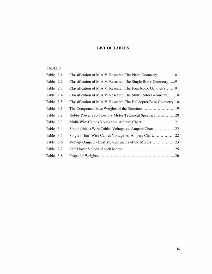
LIST OF TABLES

TABLES

Table 2.1 Classification of M.A.V. Research;The Plane Geometry………….. 8

Table 2.2 Classification of M.A.V. Research;The Single Rotor Geometry…...9

Table 2.3 Classification of M.A.V. Research;The Four Rotor Geometry……. 9

Table 2.4 Classification of M.A.V. Research;The Multi Rotor Geometry…… 10

Table 2.5 Classification of M.A.V. Research;The Helicopter Base Geometry. 10

Table 3.1 The Component base Weights of the Structure……………………. 19

Table 3.2 Robbe Power 280 Slow Fly Motor Technical Specifications……... 20

Table 3.3 Multi-Wire Cables Voltage vs. Ampere Chart…………………….. 21

Table 3.4 Single (thick) Wire Cables Voltage vs. Ampere Chart…………….. 22

Table 3.5 Single (Thin) Wire Cables Voltage vs. Ampere Chart…………….. 22

Table 3.6 Voltage-Ampere-Trust Measurements of the Motors……………… 23

Table 3.7 Self-Hover Values of each Motor………………………………….. 25

Table 3.8 Propeller Weights…………………………………………………...26

x

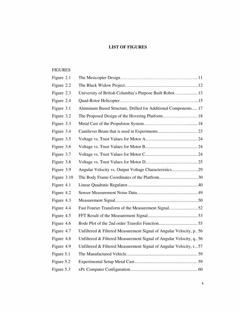
LIST OF FIGURES

FIGURES

Figure 2.1 The Mesicopter Design…………………………………………….. 11

Figure 2.2 The Black Widow Project………………………………………….. 12

Figure 2.3 University of British Columbia’s Purpose Built Robot……............. 13

Figure 2.4 Quad-Rotor Helicopter……………………………………………...15

Figure 3.1 Aluminum Based Structure, Drilled for Additional Components..... 17

Figure 3.2 The Proposed Design of the Hovering Platform…………………… 18

Figure 3.3 Metal Cast of the Propulsion System…………………………......... 18

Figure 3.4 Cantilever Beam that is used in Experiments.................................... 23

Figure 3.5 Voltage vs. Trust Values for Motor A............................................... 24

Figure 3.6 Voltage vs. Trust Values for Motor B............................................... 24

Figure 3.7 Voltage vs. Trust Values for Motor C............................................... 24

Figure 3.8 Voltage vs. Trust Values for Motor D............................................... 25

Figure 3.9 Angular Velocity vs. Output Voltage Characteristics........................ 29

Figure 3.10 The Body Frame Coordinates of the Platfrom................................... 30

Figure 4.1 Linear Quadratic Regulator................................................................ 40

Figure 4.2 Sensor Measurement Noise Data....................................................... 49

Figure 4.3 Measurement Signal...........................................................................50

Figure 4.4 Fast Fourier Transform of the Measurement Signal.......................... 52

Figure 4.5 FFT Result of the Measurement Signal............................................. 53

Figure 4.6 Bode Plot of the 2nd order Transfer Function................................... 55

Figure 4.7 Unfiltered & Filtered Measurement Signal of Angular Velocity, p.. 56

Figure 4.8 Unfiltered & Filtered Measurement Signal of Angular Velocity, q.. 56

Figure 4.9 Unfiltered & Filtered Measurement Signal of Angular Velocity, r... 57

Figure 5.1 The Manufactured Vehicle................................................................ 59

Figure 5.2 Experimental Setup Metal Cast......................................................... 59

Figure 5.3 xPc Computer Configuration............................................................. 60

xi

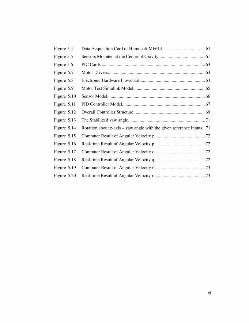
Figure 5.4 Data Acquisition Card of Humusoft MF614......................................61

Figure 5.5 Sensors Mounted at the Center of Gravity......................................... 61

Figure 5.6 PIC Cards........................................................................................... 63

Figure 5.7 Motor Drivers.....................................................................................63

Figure 5.8 Electronic Hardware Flowchart......................................................... 64

Figure 5.9 Motor Test Simulink Model...............................................................65

Figure 5.10 Sensor Model..................................................................................... 66

Figure 5.11 PID Controller Model........................................................................ 67

Figure 5.12 Overall Controller Structure.............................................................. 69

Figure 5.13 The Stabilized yaw angle................................................................... 71

Figure 5.14 Rotation about z-axis – yaw angle with the given reference inputs...71

Figure 5.15 Computer Result of Angular Velocity p............................................ 72

Figure 5.16 Real-time Result of Angular Velocity p............................................ 72

Figure 5.17 Computer Result of Angular Velocity q............................................ 72

Figure 5.18 Real-time Result of Angular Velocity q............................................ 72

Figure 5.19 Computer Result of Angular Velocity r............................................. 73

Figure 5.20 Real-time Result of Angular Velocity r............................................. 73

1

CHAPTER I

INTRODUCTION

1.1 Introduction

The flying robot is one of the emerging research topics among the unmanned

aerial vehicles. A flying robot can be defined as a hovering platform with robotic

features, which may be in different sizes and various mission capabilities. Flying

robots can be considered as sensor platforms with six-degrees of freedom. Stabilizing

and guidance of these hovering platforms are common and basic tasks that have to be

accomplished before assigning a mission to the vehicle. Several universities and

research centers have initiated flying robot projects in the level of bachelor’s, masters

and doctorate level for many years over last two decades.

Mission capability and intelligent guidance are long lasting projects in the

flying robot technology. A flying robot can have varying mission capabilities. The

major goal of this study consists of manufacturing and stabilizing of a flying robot,

which can have different capabilities for use in undergraduate laboratories. The

guidance of the vehicle along the inertial axes is not the primary concern in this

project. No other missions such as vertical take-off and landing are expected from

the hovering platform except stabilizing itself in the air with respect to its body frame

axes. The structure of the investigated aerial vehicle in this study consists of a plus

sign shape rigid geometry and four motors assembled to the end nodes of the frame.

Each motor has a gear system and a propeller to generate the required lifting force.

Three gyroscopes are used to sense the three axes rotation motions of the platform.

2

External power supplies and computer support are provided. Matlab 6.5 / Simulink

package program is used to simulate control and analyze the hovering vehicle. The

selected control algorithm is the Linear quadratic regulator and a PD controller

combined with a filter. The PD controller is used to navigate the rotation of the

vehicle about the z-axis of the body frame of the hovering vehicle. The use of low-

pass filter is investigated to eliminate the measurement noise.

1.2 What is a Flying Robot?

Before introducing the definition of a flying robot, it may be proper to first

describe and differentiate Micro Aerial Vehicles (M.A.V.) and the Unmanned Aerial

Vehicles (U.A.V.) [Michelson R. C., 2000].

A Micro Aerial Vehicle (M.A.V.) is a semiautonomous hovering vehicle, sizing less

than approximately 0.15 m in any dimension, mass about 0.115 kg, has a range of

approximately up to 10 km, and a top speed of up to 50 km/h that can accomplish an

useful military mission at an affordable cost (less than $1,000 if it is one time use

disposable system). The aerial vehicle has to be durable enough from 20 minutes to 2

hours to accomplish a given task. M.A.V. may be regarded as a sensor platform with

a "six-degrees-of-freedom" that will enable a broad spectrum of small-unit and

special operations. Missions might include video and multi-spectral (infrared)

reconnaissance and surveillance, battle-damage assessment, targeting of weapons on

key installations, placement of autonomous sensors, communication systems, or the

detection of hazardous substances or land mines. The aerial vehicle is expected to

satisfy the nominal performance goals including real-time imaging, navigation, and

communications capabilities. Other applications include monitoring hostage

situations or weapons-ban treaties, patrolling national borders, and searching for

disaster survivors. Another crucial requirement for the M.A.V. lies in its ability to

prevent itself from being seen and heard. If detected, it should not explicitly display

its presence away nor compromise the operator's location. As a result, an optimally

3

designed/configured M.A.V. has to be as close as possible to a flying sensor chip. On

the other hand, an Unmanned Aerial Vehicle (U.A.V.) can be described as a

preliminary version of a M.A.V. The above-mentioned tasks, control systems, motor

and energy unit equipments and all electronic stuff are first tested and embedded on a

U.A.V. If the requested goal is achieved in success, these new accessories and

control or design logics can be tried to be integrated on a M.A.V.

Among the specific significant engineering challenges that researchers are focusing

on for the development of successful M.A.V. and U.A.V. exist ultra-compact,

lightweight, high-power and high-energy-density propulsion and power sources;

untraditional concepts for lift generation; flight stabilization and control for

aerodynamic environments with very low Reynolds numbers; secure, low-power

onboard electronic processing and communications with sufficient bandwidth for

real-time imaging; micro-gyroscopes and inertial measurement units (I.M.U.) and

very small onboard guidance, navigation, and geo-location systems. To be really

useful, a M.A.V. needs to carry a short-range day/night area imaging system with a

sufficient resolution. The system must feature an accurate geo-location capability. A

sufficient vehicle range and real-time communications are also desired. Also, M.A.V.

has to be lightweighted and robust enough to be carried in a backpack [Keennon

M.T., 2002].

The fundamental difference between a M.A.V. and an U.A.V. is the physical size of

the vehicle. The size of all the electronic components and the overall physical

structure of a M.A.V. are smaller than the size of an U.A.V.

In general, the control architecture and core missions are similar. However, M.A.V.s

have more engineering problems because of their smaller dimensions, which can

create low-level dynamics as well as manufacturing and control problems. U.A.V.s

are being used commercially in many applications especially in military and even

also in toy industry.

4

1.3 Aim and Scope of this Research

This thesis consists of developing an U.A.V.. In 2002, the design and

manufacture of an aerial vehicle were completed as a three-month term project

within the course ME 462, at the Middle East Technical University (METU), Turkey.

Student teams in this course designed a plus sign shaped Aluminum structure with

four electrically powered, propeller based propulsion sets and a controller. The main

goal of the manufactured aerial vehicle was to stabilize itself in the hover conditions.

The structure of the U.A.V.s were around 40-45 cm in all dimensions without

propellers. An externally plugged and nearby located power source for the

mechanical system was selected for the propulsion set and the controller. The

hovering platform dynamics considered in the controller design were simplified. A

PD controller is selected to stabilize the vehicle. Maneuvering and guidance of the

aerial vehicle were not among the goals of the project. Three gyroscopes that were

located at the center of gravity sensed the mechanical structure’s rotation rates in

terms of body frame components. An off-board processor and a terminal ground

based computer communicated to process the data received by the sensors and drive

the motors. Matlab 6.5 / Simulink package program was used as the real time

controller. However, the aerial vehicle could not lift and stabilize itself.

In this thesis, a similar mechanical structure and configuration is chosen. Similar

mechanical components are used to build a more robust structure. Calculations and

tests are performed in detail to adopt the aerial vehicle to the real time environment

and to design a robust controller. A new control algorithm is chosen and applied on

the aerial vehicle. A Linear quadratic regulator (LQR) controller and a PD controller

are chosen for the considered problem. Three gyroscopes are used to sense the

system states. The six-degrees of freedom platform system that consists of inertial

measurement units can be considered as an experimental setup for undergraduate

laboratories. In laboratory, it is proposed to test the noisy environment of the plant

and sensor measurements, controllers and filter designs tools. On the other hand,

stabilizing the vehicle in the air, guidance and different mission capabilities can be

5

integrated and experimented. Such a system can assist the undergraduate students to

learn and simulate more in control systems, manufacturing and design.

During this study, it is observed that the three gyroscopic sensors are not enough for

such an unmanned aerial vehicle project. For a six-degree of freedom system, the

vehicle motion in all directions about and along the body frame axes have to be

measured for a complete navigation and guidance. An observability problem arises

when there are unmeasured states. In this study, some of the governing states of the

equations of motion can not be measured. The foregoing observability problem is

considered. The sensed plant and measurement noises of the aerial vehicle are not

omitted during computer simulations and real time experiments. The effects of the

disturbances/noises are taken into consideration. Flat earth, principal axes and rigid

vehicle frame assumptions are made to simplify the leading motion equations. A

low-pass filter is designed to reduce the system noise and adapted to the aerial

vehicle in real time. Matlab 6.5 / Simulink software is used to process the received

sensor data and simulate the aerial vehicle behavior on the computer. As a result,

stabilization of the manufactured aerial vehicle in the air is successfully

accomplished. Additionally, a PD controller navigates the yaw angle of the vertical

axis of the body frame of the hovering vehicle.

1.4 Outline

The rest of the thesis is organized as follows. Chapter II presents a literature

review of the state-of-the-art in three main subjects, namely overview, developing

technologies on M.A.V. and U.A.V. and comparison of some promising projects in

detail. In Chapter III, the physical component design, manufacture and selection

steps are outlined. The DC motor, gear and propeller selections are detailed.

Experimental tests are given. An overview of the mathematical model, governing

equations and force relations are developed. In Chapter IV, Linear quadratic

regulator controller is given in detail. The observability and controllability are

6

checked. Various filter designs are proposed to overcome the noise problem of the

plant and the sensor measurement noises. In Chapter V, the experimental setup is

defined. A computer simulation is performed and its experimental results are

investigated. In the last chapter, the results and future work are stated.

7

CHAPTER II

THE UNMANNED AERIAL VEHICLE PROJECTS

2.1 Overview

It is apparent that each discipline of engineering has different approaches to

M.A.V. and U.A.V.. Especially, mechanical engineers, electric-electronic engineers,

aerospace engineers have a great interest in manufacturing and controlling of these

aerial vehicles. Mechanical engineers focus on manufacturing of the aerial vehicle

structure, mathematical modeling and controller design. Moreover, reducing the

mass of the components, researching new power sources and manufacturing the

smallest mechanical hardware are other crucial research topics for mechanical

engineers. Electric-electronic engineers prefer to study on already-manufactured

mechanism like remote control (R/C) planes or helicopters and focus on the

controller design, inertial measurement units, new power units and power

consumption optimization. Aerospace engineers, especially consider the problem of

designing sub-power systems like propeller manufacturing, low Reynold’s number

behaviors, aerodynamic effects and flight dynamics. Other disciplines of sciences

like statistics and industrial engineering contribute to the problem in the context of

computer algorithms, mathematical modeling, controller design and logics, and

component based optimization tools.

8

2.2 Developing Technologies on M.A.V. and U.A.V.

It is possible to classify the previous researches on M.A.V and U.A.V.

according to the structural, mechanical, sensory equipment or proposed mission

goals. Every mechanical component or controller specification, which is a

distinguishable aspect for such aerial vehicles, has its own technological

development. Thus, different comparisons can be performed among each hardware

and software of the aerial vehicles. In this study, the classification is based on the

structural design and propulsion types of the vehicles that were previously studied.

The comparisons are summarized in the Tables 2.1 to 2.5. Currently, there are many

propulsion type alternatives available. Among the most widely used propulsion type

alternatives, the best ones are the propeller power, fuel power, gas power and

flapping wing power. The selection of the propulsion type is based on the structure

preferred. On the other hand, the selected comparison criteria for the aerial vehicles

affect many other specifications. As an example, the criteria based on the number of

sensors used affect the controller selection. Also, the capacity of the power source

deduces the hover time of the vehicle. The propulsion type directly affects the

structural geometry of the hovering vehicles.

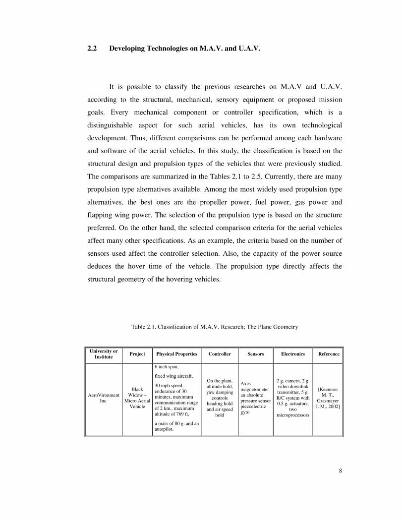
Table 2.1. Classification of M.A.V. Research; The Plane Geometry

University or Institute Project Physical Properties Controller Sensors Electronics Reference

AeroVironment Inc.

Black Widow –

Micro Aerial Vehicle

6 inch span,

fixed wing aircraft,

30 mph speed, endurance of 30 minutes, maximum communication range of 2 km., maximum altitude of 769 ft,

a mass of 80 g. and an autopilot.

On the plant, altitude hold, yaw damping

controls heading hold and air speed

hold

Axes magnetometer an absolute pressure sensor piezoelectric gyro

2 g. camera, 2 g. video downlink transmitter, 5 g. R/C system with 0.5 g. actuators,

two microprocessors

[Keennon M. T.,

Grasmayer J. M., 2002]

9

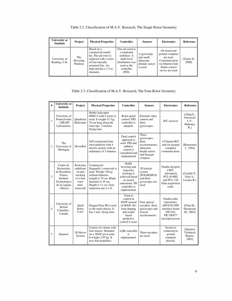
Table 2.2. Classification of M.A.V. Research; The Single Rotor Geometry


University of Reading, U.K.

The Hovering Platform

Based on a commercial model kit. The tail rotor is replaced with a series of four laterally mounted fins. 1m high and has a 1.5 m diameter.

Fins are used as a rotational stabilizer. A multi level

distribution was used as the controller

(PID).

A gyroscope and small ultrasonic altitude sensor is used.

On board and ground computer

are used. Communication via Ethernet link.

Radio control servos are used.

[Taylor D, 2000]

Table 2.3. Classification of M.A.V. Research; The Four-Rotor Geometry

# University or Institute Project Physical Properties Controller Sensors Electronics Reference

1

University of Pennsylvania

– GRASP Laboratories

Quadrotor Helicopter

Hobby helicopter HMX-4 with 4 rotors is used. It weighs 0.7 kg. 76 cm long along the rotor tips. 3 minutes flying time.

Rotor speed control. PID controller is

adopted.

External video camera and three gyroscopes.

R/C receiver

[Altu� E., Ostrowski

J. P., Mahoney

R.]

2 The

University of Michigan

HoverBot

Self constructed four-rotor platform with 4 electric motors with an endurance of 3 minutes.

Dual control approach is

used. PID and additive

control is considered and implemented

Three gyroscopes, three accelerometers, ultrasonic height sensor and fluxgate compass.

4 Channel R/C unit for ground

computer communication.

[Borenstein J., 1994]

3

Centre de Recherches

de Royallieu-France

Instituto Technologico de la Laguna

– Mexico

Real-time stabilizati

on and tracking of a four

rotor mini-

rotorcraft

Commercial Draganfly’s rotorcraft is used. Weighs 320 gr without batteries. Length is 74 cm. Blade diameter is 29 cm. Height is 11 cm. Gear reduction rate is 1:6.

Stable hovering and

trajectory tracking is

achieved based on nested

saturations. PD controller is

implemented.

3D tracker system (POLHEMUS) and three gyroscopes are used.

Fatuba skysport 4 R/C,

Advantech PCL-818HG and PCL-726

Data acquisition cards.

[Castillo P., Dzul A.,

Lozano R.]

4

University of British

Columbia - Canada

Quad Rotor UAV

Dragan Flyer III is used as the main chassis. It has 3 min. flying time.

Tried to control in

2DOF instead of 6DOF. H� loop shaping and model

based predictive

control is used.

Four optical encoders, three gyroscopes and triaxial accelerometer.

Fatuba radio transmitter,

dSPACE DSP interface board

DS1102, PIC16F877

microprocessors

[Chen M., Huzmezan M., 2003]

5 Quanser 3D Hover System

Consist of a frame with four motors. Mounted on a 3DOF pivot joint. It weighs 2.85 kg. It uses 8x6 propellers.

LQR controller is

implemented.

Three encoders are used.

System is connected to

ground computer directly.

[Quanser Technical Report, 2002]

10

Table 2.4. Classification of M.A.V. Research; The Multi-Rotor Geometry


University of British

Columbia , Canada

A Purpose Built Robot

It consists of seven propellers. One main propeller centered around six small control propellers. Powered by 17 hp engine. Belt system is used to distribute the power.

Separate PID controller for

each degree of freedom. They

have implemented a

H� on the plant.

Inertial gyroscope, differential GPS unit, fluxgate compass and a sonar is used.

High-resolution camera. On

board ad ground control stations. Communication

via wireless modem module.

[Gibb J., Jones C., Lee T., 2001]

Table 2.5. Classification of M.A.V. Research; The Helicopter Base Geometry


Circuit Cellar Internet Control

3 DOF helicopter model is used. External power system is provided.

LQR controller is implemented.

Optical encoders are used.

Data acquisition and controller board is used.

[Apkajian J., 1999]

2.3 Comparison of Some Promising Projects in Detail

Different aerial vehicle projects are being studied in many universities,

research institutes and commercial organizations. These projects differ

approximately in every mechanical component and controller design from each

other. Each research group tries to make an untraditional vehicle in some aspect. It is

possible to group these projects into categories to study in detail. The premier

categorization can be in the structural design. Each research group manufactures

their own structural design. These designs vary according to the proposed mission.

Large structures are preferred for outdoor applications while the smaller ones are

used for the spy games. The structural selection and manufacturing of the hovering

vehicle is a result of experience and aim.

11

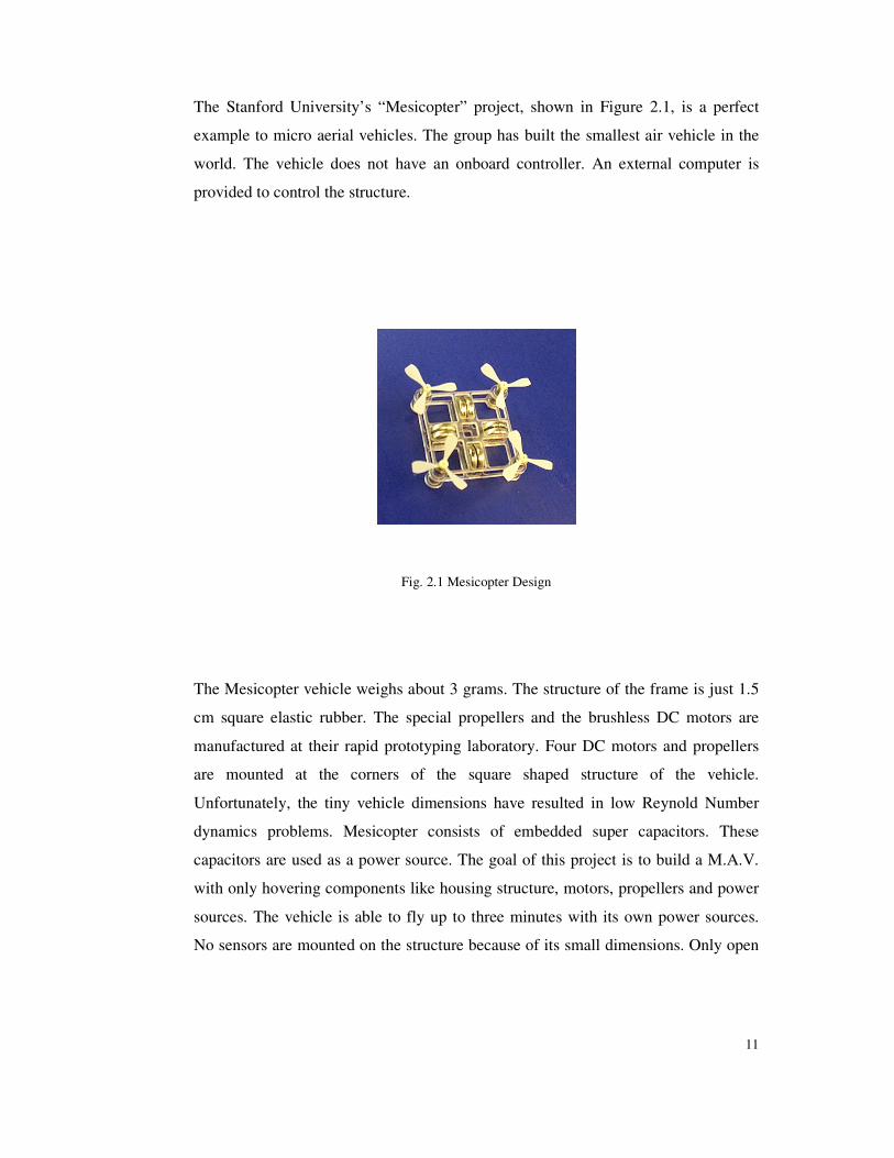
The Stanford University’s “Mesicopter” project, shown in Figure 2.1, is a perfect

example to micro aerial vehicles. The group has built the smallest air vehicle in the

world. The vehicle does not have an onboard controller. An external computer is

provided to control the structure.

Fig. 2.1 Mesicopter Design

The Mesicopter vehicle weighs about 3 grams. The structure of the frame is just 1.5

cm square elastic rubber. The special propellers and the brushless DC motors are

manufactured at their rapid prototyping laboratory. Four DC motors and propellers

are mounted at the corners of the square shaped structure of the vehicle.

Unfortunately, the tiny vehicle dimensions have resulted in low Reynold Number

dynamics problems. Mesicopter consists of embedded super capacitors. These

capacitors are used as a power source. The goal of this project is to build a M.A.V.

with only hovering components like housing structure, motors, propellers and power

sources. The vehicle is able to fly up to three minutes with its own power sources.

No sensors are mounted on the structure because of its small dimensions. Only open

12

loop control can be performed. Development of inertial measurement units for tiny

vehicle dimensions is being studied. [Kroo I., 2001]

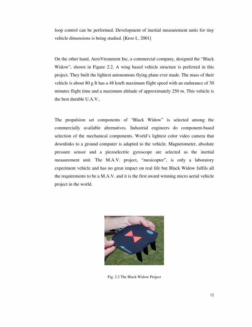
On the other hand, AeroVironment Inc, a commercial company, designed the “Black

Widow”, shown in Figure 2.2. A wing based vehicle structure is preferred in this

project. They built the lightest autonomous flying plane ever made. The mass of their

vehicle is about 80 g It has a 48 km/h maximum flight speed with an endurance of 30

minutes flight time and a maximum altitude of approximately 250 m. This vehicle is

the best durable U.A.V..

The propulsion set components of “Black Widow” is selected among the

commercially available alternatives. Industrial engineers do component-based

selection of the mechanical components. World’s lightest color video camera that

downlinks to a ground computer is adapted to the vehicle. Magnetometer, absolute

pressure sensor and a piezoelectric gyroscope are selected as the inertial

measurement unit. The M.A.V. project, “mesicopter”, is only a laboratory

experiment vehicle and has no great impact on real life but Black Widow fulfils all

the requirements to be a M.A.V. and it is the first award winning micro aerial vehicle

project in the world.

Fig. 2.2 The Black Widow Project

13

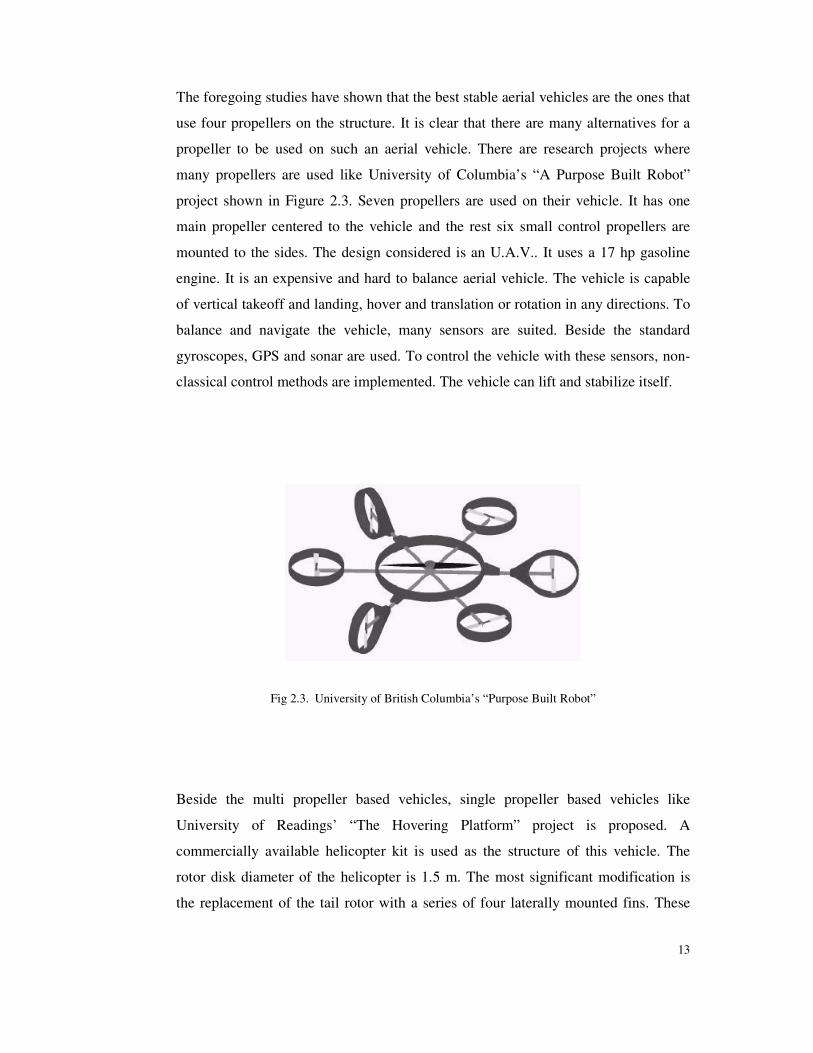
The foregoing studies have shown that the best stable aerial vehicles are the ones that

use four propellers on the structure. It is clear that there are many alternatives for a

propeller to be used on such an aerial vehicle. There are research projects where

many propellers are used like University of Columbia’s “A Purpose Built Robot”

project shown in Figure 2.3. Seven propellers are used on their vehicle. It has one

main propeller centered to the vehicle and the rest six small control propellers are

mounted to the sides. The design considered is an U.A.V.. It uses a 17 hp gasoline

engine. It is an expensive and hard to balance aerial vehicle. The vehicle is capable

of vertical takeoff and landing, hover and translation or rotation in any directions. To

balance and navigate the vehicle, many sensors are suited. Beside the standard

gyroscopes, GPS and sonar are used. To control the vehicle with these sensors, non-

classical control methods are implemented. The vehicle can lift and stabilize itself.

Fig 2.3. University of British Columbia’s “Purpose Built Robot”

Beside the multi propeller based vehicles, single propeller based vehicles like

University of Readings’ “The Hovering Platform” project is proposed. A

commercially available helicopter kit is used as the structure of this vehicle. The

rotor disk diameter of the helicopter is 1.5 m. The most significant modification is

the replacement of the tail rotor with a series of four laterally mounted fins. These

14

fins are used as a part of the rotational stability feedback loop to counteract the

rotational forces applied to the body of the aircraft during flight. The fins are

mounted on the platform at an angle directly underneath the main rotors. A small

ultrasonic altitude sensor and a small solid-state gyroscope are used to sense the

elevation and rotation rates. These fins are used to transform energy from the

downdraft produced by motor blades into a torque on the body of the hovering

platform. Two experiments are conducted on the vehicle to test if the vehicle can

hover or not resulting with a failure and a success. The clever idea of hovering

mechanism of the project needs more experiments to be more robust. Using four

propellers on an unmanned aerial vehicle is a general approach. This geometry and

rotational array of design are easy to implement, stabilize and control rather that the

other alternatives. Increasing or decreasing the motor voltages simply stabilizes and

guide the vehicles. Four-rotor rotational array geometry is simple and efficient for

propeller-based designs. University of Pennsylvania’s “Quadrotor helicopter”

project, The University of Michigan’s “HoverBot” and Centre de Recherches de

Royallieu –France’s “Rotorcraft” projects are simple examples to this claim. Plus

sign shape geometry is another common aspect for all three aerial vehicles. The DC

motors and propellers are similar, too.

All three of the projects have their own onboard power supply and have a similar

flight time of approximately three minutes. The lightest one is the “Rotorcraft”

project. Its mass is 0.5 kg while the heaviest one is the “Quadrotor” project with its

0.8 kg mass. PD controller is a common controller for three of the vehicles. The most

robust one is the “HoverBot” project. The “HoverBot” vehicle consist of three

gyroscopes, three accelerometers, ultra sonic height sensor and a flux gate compass

while the quadrotor has only an external camera and three onboard gyroscopes and

rotorcraft consists of a tracker system and three gyroscopes.

It is possible to say that, using many sensors increase the robustness of the

implemented controller to the vehicle. Increasing the number of sensors used in the

vehicle eliminates the observability problem and avoids using difficult and hard to

implement controller algorithms for the aerial vehicles. Additionally, “Rotorcraft”

15

team has reported that one cannot stabilize a hovering vehicle with only three

gyroscopes [Chen M., Huzmezan M., 2003]. Usually, hovering platforms are six

degrees of freedom motion vehicles and to control the vehicle the states have to be

observed. The number of sensors is directly related with which states can be

estimated and observed. Affordability of these sensor devices is the cost of using

many sensors. The “HoverBot” project is the most expensive system among the other

alternatives.

Fig 2.4 Quad-Rotor Helicopter

A common approach in designing aerial vehicles is to use commercially available

helicopter kit structures. Generating the required thrust force for hovering is not a

crucial task for these helicopter kit structures. Gasoline powered engines and

propellers with approximate radius of 2 m provide the necessary power for hovering

and navigating. Different competitions among these aerial vehicle developer groups

are made in every year around the world. The competitors are required to complete

the given missions.

16

CHAPTER 3

STRUCTURAL DESIGN, COMPENENT-BASED SELECTION AND

ANALYSIS

The ME 462 course project student teams built their own four-rotor hovering

vehicles, which are similar to previously mentioned four-rotor type aerial vehicles.

The ME 462 course project was the frontier model, which was examined on hovering

vehicles. In this thesis, a new and robust four-rotor structure is proposed and built.

The structural frame of the aerial vehicle is similar to its alternatives previously built

in ME 462 course project. The designed structure of the vehicle was manufactured

with the mechanical and electronical components that are already available at the

M.E.T.U. control laboratory. The power unit, which consists of a DC motor,

propeller and a gearbox was assembled. The sensory equipment was mounted. The

system was not tuned or prepared to flight in the level of manufacturing. A brief

summary is given about the manufacturing levels of the vehicle in this chapter. The

mechanical design of the vehicle is split into categories of overall structure, motor,

power system, gear, propeller and sensory equipment. The structural design and

governing mathematical equation parameter calculations were performed in

AutoCAD 2002 computer package program.

17

3.1 Structure

The previous studies in the literature and the experience on the ME 462

course project have shown that, the best geometry for such a hovering platform

project is the plus sign shape geometry. Alternative vehicle geometries are not

proposed in this thesis and it was decided to use the plus sign shape that had been

used in ME 462 projects. The stability of the plus sign frame geometry and its simple

equations of motion were an advantage during this first time hovering platform

demonstration. On the other hand, manufacturing the vehicle in plus sign shape

geometry is quite easy. Four power units that are attached to the end nodes of the

plus sign shape is the best and common array in these vehicles. Triangular array of

power units on the structure, single rotor or multi propeller power units are hard to

manufacture, balance and control. For the sake of this thesis, it is decided to build the

hovering vehicle in four-rotor type, which consist the use of Aluminum, rectangular

shell tubes in the structure given in the Figure 3.1. An overall design of the hovering

vehicle is shown in Figure 3.2. The Aluminum tubes, which are use in the structure,

have a length of 500 mm and a shell thickness of 1 mm. Also, there are other rod

material alternatives. Carbon tubes are a strong choice as a structural material. The

reason of using carbon as rod material is its super lightweight and strength against

impacts. The Aluminum-based structure has a low payload on vehicle mass and as

rigid as to carry the power and the control units. The total mass of the Aluminum

rods is 115 g.

Fig. 3.1 Aluminum based structure, drilled for additional components.

18

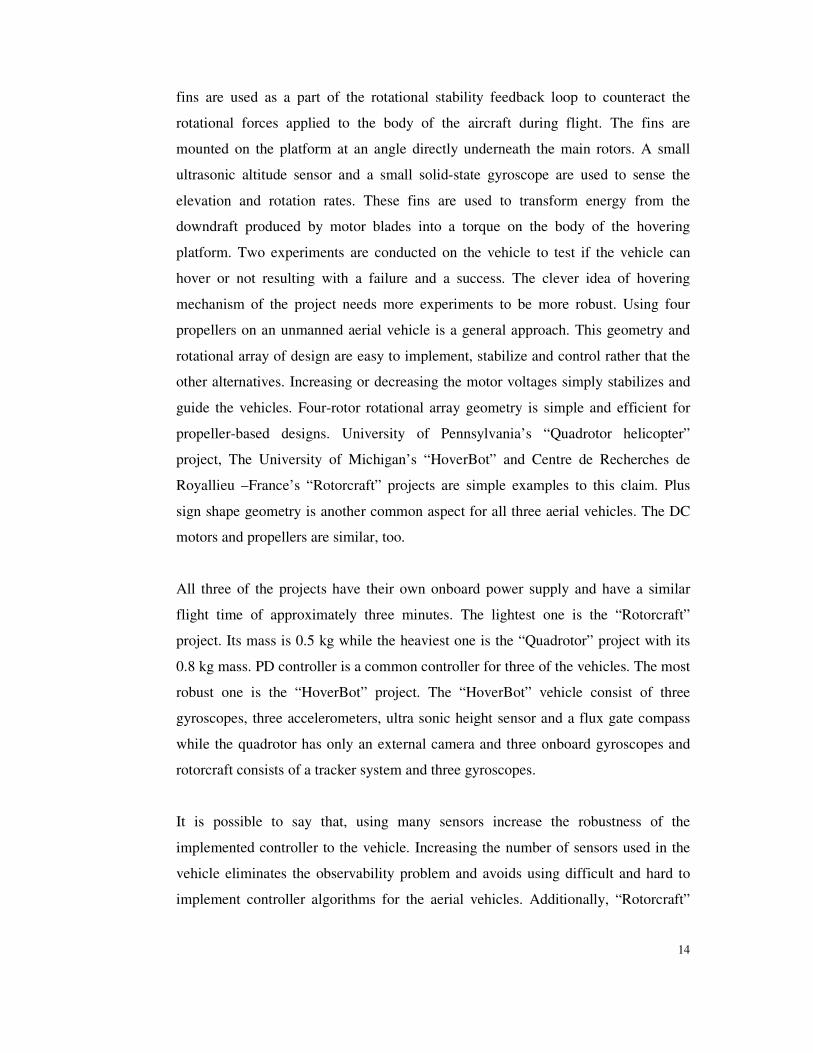
Fig 3.2.The Proposed Design of the Hovering Platform.

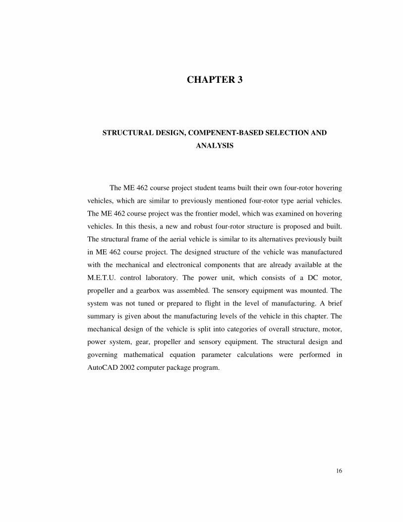
The vehicle dimensions are kept in the limits of the premier studies. The metal

housing of the motor/gear/propeller unit is heavier than other housing alternatives

such as plastic. The metal cast is preferred because of its higher rigidity and

reliability. The illustration of the metal cast is shown in Figure 3.3. A steel rod is

used to house the propeller, propeller’s metal plate and driver gear to the metal cast

by two small bearings. All the mechanical components are connected by bolts to the

metal cast. The upper part of the steel rod is toothed to hold the propeller’s

Aluminum plate. The propeller is also connected to this plate by three bolts.

Fig. 3.3 Metal Cast of the Propulsion System.

Propeller

Metal Cast

Gear

Pinion DC Motor

Bolts

Steel Rod

19

The power source for the DC motors is not placed on the vehicle because of the mass

limitations. External power supply that can provide 12 Volts supported by 12

Ampere is sufficient for such a hovering vehicle project. Placing power equipments

like cellular battery packs on the vehicle can be possible if lighter and efficient DC

motors can be used. Matlab 6.5 / Simulink package program is preferred to control

and simulate the hovering platform in real time by a data acquisition card. Motor

drivers were built to link between the DC motors and the PIC cards of the system.

These drivers were used to control the voltage inputs by computer. The control

architecture will be explained in the next chapter. Also, the following assumptions

are made for developing the mathematical equations of the hovering vehicle;

• Rigid airframe,

• Flat Earth (i.e. gravity is taken to be in the vertical z direction with

respect to world fixed frame),

• Cartesian coordinates are fixed to the vehicle’s center of gravity ,

• Earth-fixed reference frame is treated as the inertial reference frame,

• The body frame is assumed to be the principal frame thus the inertia

matrix has only the diagonal elements.

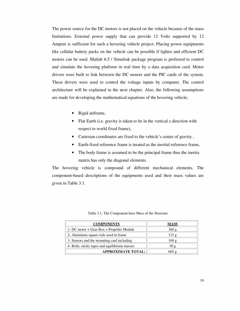
The hovering vehicle is compound of different mechanical elements. The

component-based descriptions of the equipments used and their mass values are

given in Table 3.1.

Table 3.1. The Component-base Mass of the Structure

COMPONENTS MASS 1- DC motor + Gear Box + Propeller Module 360 g 2- Aluminum square rods used in frame 115 g

3- Sensors and the mounting card including 100 g 4- Bolts, sticky tapes and equilibrium masses 30 g

APPROXIMATE TOTAL: 605 g

20

3.1.1 Motors

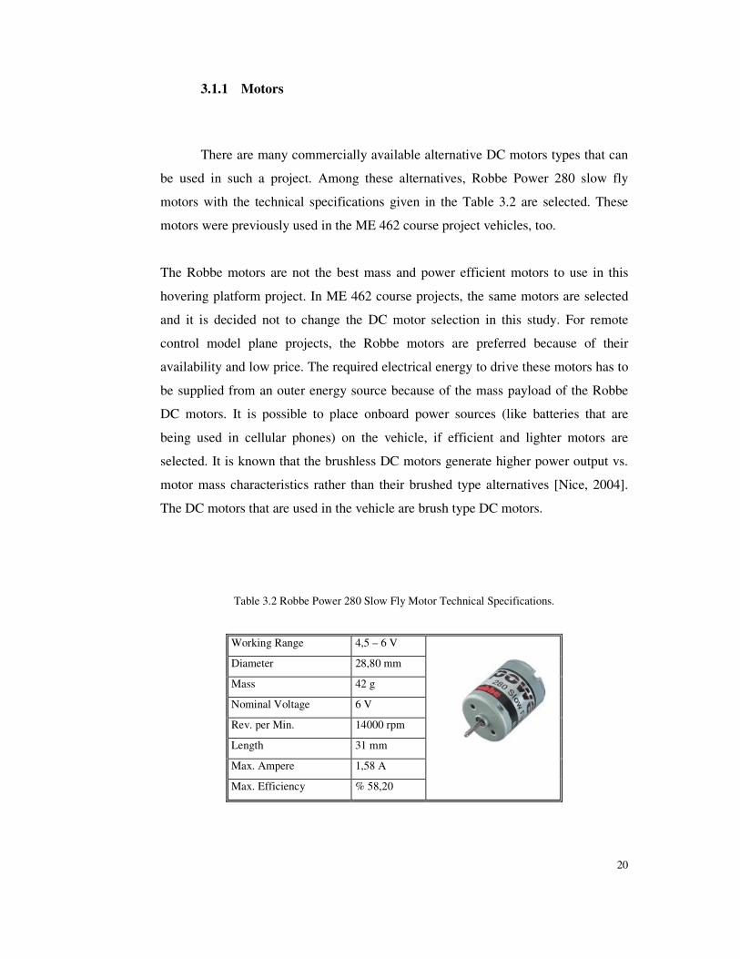
There are many commercially available alternative DC motors types that can

be used in such a project. Among these alternatives, Robbe Power 280 slow fly

motors with the technical specifications given in the Table 3.2 are selected. These

motors were previously used in the ME 462 course project vehicles, too.

The Robbe motors are not the best mass and power efficient motors to use in this

hovering platform project. In ME 462 course projects, the same motors are selected

and it is decided not to change the DC motor selection in this study. For remote

control model plane projects, the Robbe motors are preferred because of their

availability and low price. The required electrical energy to drive these motors has to

be supplied from an outer energy source because of the mass payload of the Robbe

DC motors. It is possible to place onboard power sources (like batteries that are

being used in cellular phones) on the vehicle, if efficient and lighter motors are

selected. It is known that the brushless DC motors generate higher power output vs.

motor mass characteristics rather than their brushed type alternatives [Nice, 2004].

The DC motors that are used in the vehicle are brush type DC motors.

Table 3.2 Robbe Power 280 Slow Fly Motor Technical Specifications.

Working Range 4,5 – 6 V

Diameter 28,80 mm

Mass 42 g

Nominal Voltage 6 V

Rev. per Min. 14000 rpm

Length 31 mm

Max. Ampere 1,58 A

Max. Efficiency % 58,20

21

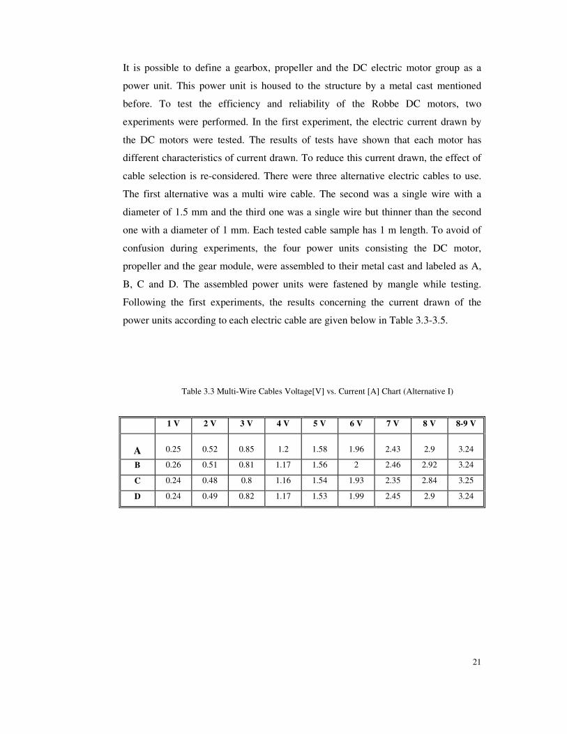
It is possible to define a gearbox, propeller and the DC electric motor group as a

power unit. This power unit is housed to the structure by a metal cast mentioned

before. To test the efficiency and reliability of the Robbe DC motors, two

experiments were performed. In the first experiment, the electric current drawn by

the DC motors were tested. The results of tests have shown that each motor has

different characteristics of current drawn. To reduce this current drawn, the effect of

cable selection is re-considered. There were three alternative electric cables to use.

The first alternative was a multi wire cable. The second was a single wire with a

diameter of 1.5 mm and the third one was a single wire but thinner than the second

one with a diameter of 1 mm. Each tested cable sample has 1 m length. To avoid of

confusion during experiments, the four power units consisting the DC motor,

propeller and the gear module, were assembled to their metal cast and labeled as A,

B, C and D. The assembled power units were fastened by mangle while testing.

Following the first experiments, the results concerning the current drawn of the

power units according to each electric cable are given below in Table 3.3-3.5.

Table 3.3 Multi-Wire Cables Voltage[V] vs. Current [A] Chart (Alternative I)

1 V 2 V 3 V 4 V 5 V 6 V 7 V 8 V 8-9 V

A 0.25 0.52 0.85 1.2 1.58 1.96 2.43 2.9 3.24

B 0.26 0.51 0.81 1.17 1.56 2 2.46 2.92 3.24

C 0.24 0.48 0.8 1.16 1.54 1.93 2.35 2.84 3.25

D 0.24 0.49 0.82 1.17 1.53 1.99 2.45 2.9 3.24

22

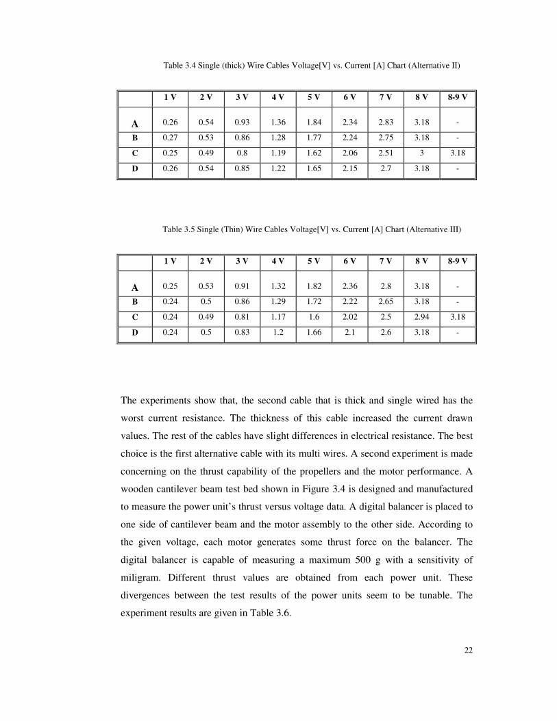
Table 3.4 Single (thick) Wire Cables Voltage[V] vs. Current [A] Chart (Alternative II)

1 V 2 V 3 V 4 V 5 V 6 V 7 V 8 V 8-9 V

A 0.26 0.54 0.93 1.36 1.84 2.34 2.83 3.18 -

B 0.27 0.53 0.86 1.28 1.77 2.24 2.75 3.18 -

C 0.25 0.49 0.8 1.19 1.62 2.06 2.51 3 3.18

D 0.26 0.54 0.85 1.22 1.65 2.15 2.7 3.18 -

Table 3.5 Single (Thin) Wire Cables Voltage[V] vs. Current [A] Chart (Alternative III)

1 V 2 V 3 V 4 V 5 V 6 V 7 V 8 V 8-9 V

A 0.25 0.53 0.91 1.32 1.82 2.36 2.8 3.18 -

B 0.24 0.5 0.86 1.29 1.72 2.22 2.65 3.18 -

C 0.24 0.49 0.81 1.17 1.6 2.02 2.5 2.94 3.18

D 0.24 0.5 0.83 1.2 1.66 2.1 2.6 3.18 -

The experiments show that, the second cable that is thick and single wired has the

worst current resistance. The thickness of this cable increased the current drawn

values. The rest of the cables have slight differences in electrical resistance. The best

choice is the first alternative cable with its multi wires. A second experiment is made

concerning on the thrust capability of the propellers and the motor performance. A

wooden cantilever beam test bed shown in Figure 3.4 is designed and manufactured

to measure the power unit’s thrust versus voltage data. A digital balancer is placed to

one side of cantilever beam and the motor assembly to the other side. According to

the given voltage, each motor generates some thrust force on the balancer. The

digital balancer is capable of measuring a maximum 500 g with a sensitivity of

miligram. Different thrust values are obtained from each power unit. These

divergences between the test results of the power units seem to be tunable. The

experiment results are given in Table 3.6.

23

Fig. 3.4 The cantilever beam used in experiments.

Table 3.6 Voltage[V]- Current[A]-Thrust Measurements of the Power Units.

1 2 3 4 5 6 7 8 >8

T A T A T A T A T A T A T A T A T A

A 4.5-

4.8 0.25

21.5-

22 0.53

45.4-

46 0.91

75.8-

76.2 1.32

109.5-

111 1.82

142-

145 2.36

177-

178 2.8

200-

201

3.18

(7.8

V)

B 4.8-

5.3 0.24

20.9-

21.4 0.5

45.2-

45.5 0.86

77.7-

78.3 1.29

109-

111.9 1.72

145-

146 2.22

176.7-

177.5 2.65

209-

211 3.18

C 3.9-

4.2 0.24

21-

21.5 0.49

44-

45 0.81

74-

75 1.17

108.5-

109 1.6

142-

143 2.02

180-

181 2.5

212-

214 2.94

230-

231

3.18

(8.7

V)

D 4.1-

4.6 0.24

20.5-

21.3 0.51

44-

45 0.82

75.3-

76.7 1.23

110-

111 1.74

143-

145 2.12

179-

181 2.6

206-

209 3.18

T: All thrust values are in 310− Newton [N] .

A: Ampere value.

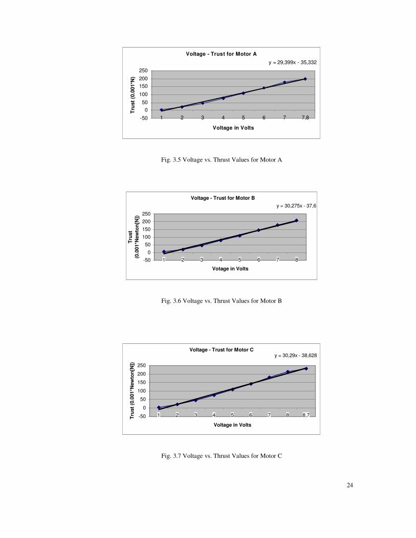
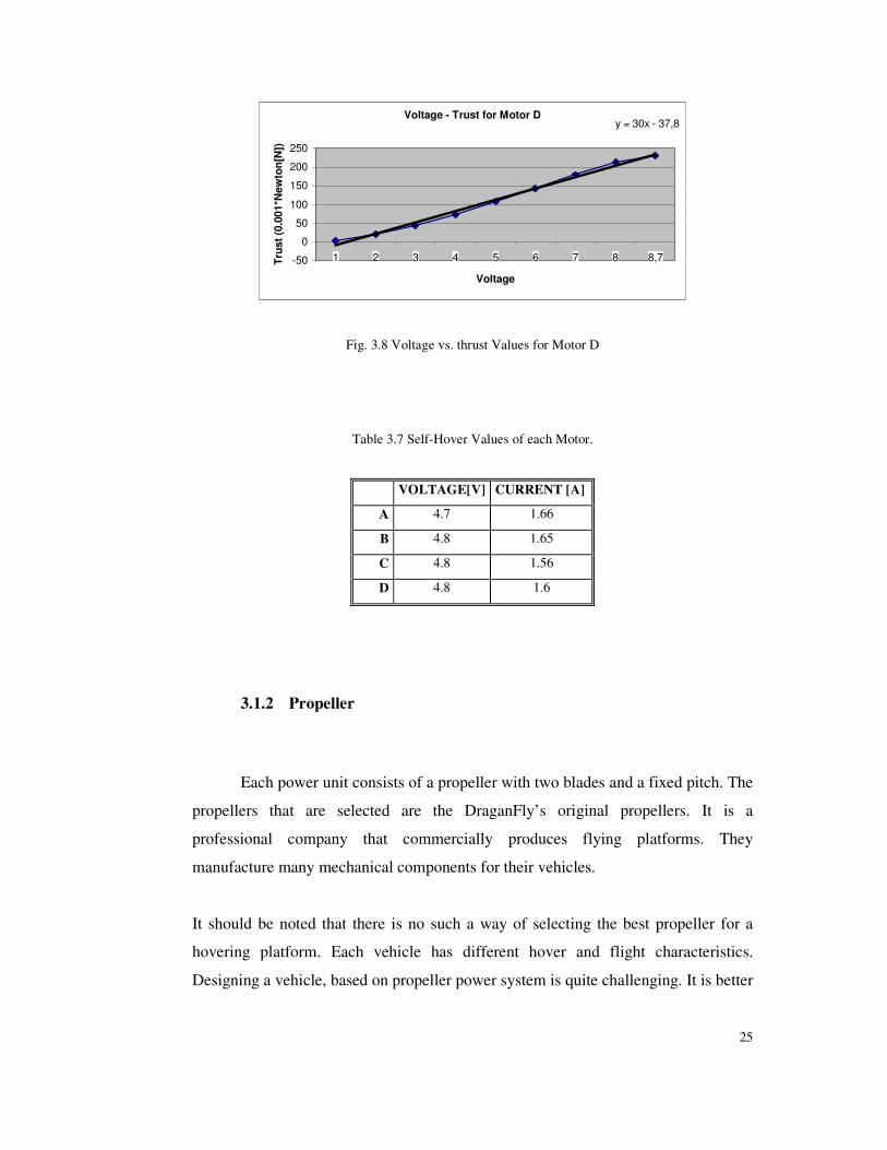
It should be noted that without counter balancing mass, the power units can balance

themselves at specific voltage values given in Table 3.7. The voltages vs. thrust

values of the motors are converted to linear equations to use in computer simulations

given in Figure 3.5-3.8.

24

Voltage - Trust for Motor A

y = 29,399x - 35,332

-50

050

100

150200250

1 2 3 4 5 6 7 7,8

Voltage in VoltsT

rust

(0.

001*

N)

Fig. 3.5 Voltage vs. Thrust Values for Motor A

Voltage - Trust for Motor By = 30,275x - 37,6

-500

50100150

200250

1 2 3 4 5 6 7 8

Votage in Volts

Trus

t (0

.001

*New

ton[

N])

Fig. 3.6 Voltage vs. Thrust Values for Motor B

Voltage - Trust for Motor Cy = 30,29x - 38,628

-50

0

50

100

150

200

250

1 2 3 4 5 6 7 8 8,7

Voltage in Volts

Trus

t (0.

001*

New

ton[

N])

Fig. 3.7 Voltage vs. Thrust Values for Motor C

25

Voltage - Trust for Motor Dy = 30x - 37,8

-50

0

50

100

150

200

250

1 2 3 4 5 6 7 8 8,7

VoltageTr

ust (

0.00

1*N

ewto

n[N

])

Fig. 3.8 Voltage vs. thrust Values for Motor D

Table 3.7 Self-Hover Values of each Motor.

VOLTAGE[V] CURRENT [A]

A 4.7 1.66

B 4.8 1.65

C 4.8 1.56

D 4.8 1.6

3.1.2 Propeller

Each power unit consists of a propeller with two blades and a fixed pitch. The

propellers that are selected are the DraganFly’s original propellers. It is a

professional company that commercially produces flying platforms. They

manufacture many mechanical components for their vehicles.

It should be noted that there is no such a way of selecting the best propeller for a

hovering platform. Each vehicle has different hover and flight characteristics.

Designing a vehicle, based on propeller power system is quite challenging. It is better

26

and convenient to make the propeller selection based on testing the propeller. In

many applications, the propeller manufacturer’s data did not match to the one that is

obtained in the laboratory experiments. As a result, one who wants to build such a

hovering platform has to make his own propeller tests. There are also many different

alternative propellers commercially available. Remote control model planes use

different types of propellers. These propellers are plastic and brittle. They are all

rigid with their fixed pitch but using rigid propellers is not effective. Stiffness of the

propellers does not let the vehicle to take off itself. On the other hand, Draganfly’s

propellers are carbon leaf based and very flexible. For this type of propellers, it is

possible to change the pitch angle even by hand. The flexibility of the propeller

results in a high thrust generation. DraganFly’s propellers have a large diameter to

accelerate the air. The alternative propellers have smaller diameters.

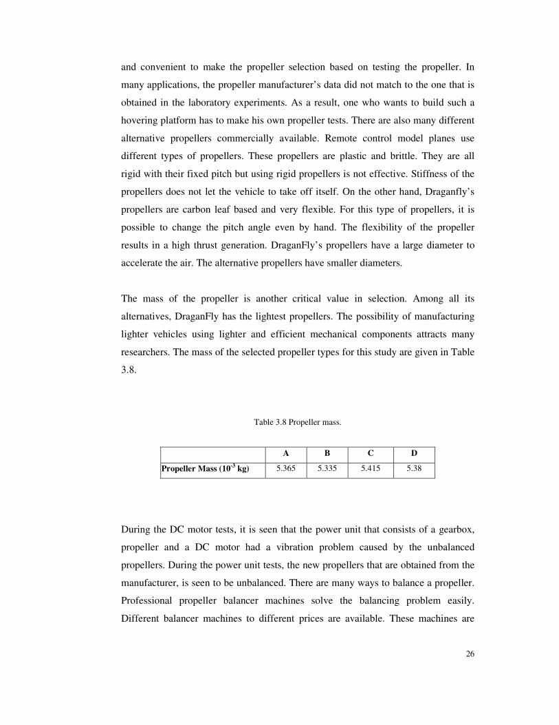
The mass of the propeller is another critical value in selection. Among all its

alternatives, DraganFly has the lightest propellers. The possibility of manufacturing

lighter vehicles using lighter and efficient mechanical components attracts many

researchers. The mass of the selected propeller types for this study are given in Table

3.8.

Table 3.8 Propeller mass.

A B C D

Propeller Mass (10-3 kg) 5.365 5.335 5.415 5.38

During the DC motor tests, it is seen that the power unit that consists of a gearbox,

propeller and a DC motor had a vibration problem caused by the unbalanced

propellers. During the power unit tests, the new propellers that are obtained from the

manufacturer, is seen to be unbalanced. There are many ways to balance a propeller.

Professional propeller balancer machines solve the balancing problem easily.

Different balancer machines to different prices are available. These machines are

27

preferred to use in sensitive applications. In this study, there is no need to use a

balancer.

The balancing of the propellers is made by hand in this project. To balance the

propellers, axial moment generation due to mass of each blade has to be considered.

A needle is mounted on a mangle horizontally. It is convenient to model the propeller

axes as the x-axis lies along the right blade, y-axis lies along the centrifugal line and

the z-axis is directed upward. Each propeller is placed on the needle at their proposed

center of gravity where it is fastened to the DC motors.

The balancing of the propellers is nothing more then removing some particles over

the blade surface. The removing of the particles is made using emery paper. The

propeller is placed perpendicular to the needle and horizontal to the ground.

According to the heaviest blade, the propeller starts to rotate with respect to the

needle. It stops rotating when the moment generated by each blade is equal with

respect to the needle. This is a balancing technique according to the z-axis of the

propellers. When this step completed, another balancing has to be considered. Next is

the balancing according to the y-axis of the propeller. If a satisfactory equilibrium is

observed, it is possible to say that the propeller is balanced according to human eye.

More sensitive balance can be made, but the balancer machines have to be preferred.

One should keep in mind that while emerying such a blade; he has to pay attention

not to change the blade’s pitch angle. The pitch angle can be changed if emerying is

applied to the bottom of the propeller blade. As a summary, balancing the propeller

from its z-axis tells which blade has a mass additive and balancing the y-axis tells

which part of the blade you have to emery. Another important part is the attack angle

side of the propeller blades has to emeried, smoothly. This will affect the lifting

capability of the propellers.

28

3.1.3 Gear System

A gear module is used to accelerate the air efficiently in the vehicle. If no

gear module is used then power unit do not provide the required thrust force. It

should be noted that increasing the motor speed reduces the torque generated. To

accelerate the air particles over the propeller blades, one has to generate higher

torques rather than speed. The magnitude of the blade diameter is related to the

volume of air accelerated. Researchers examined that the best gear reduction ratio for

such a system to generate the required or the necessary torque is greater than 6.5:1.

[Nice, 2004] Using a greater ratio than 6.5:1 would provide slight higher efficiencies

to the vehicle. The gear system that is used in this study provides a 4.8:1

transmission ratio, which is sufficient for the purpose. The gear elements have plastic

material. The selected gear system has two components with a common module of

0.5 and teeth numbers of N1=10 and N2=48. In this project, the gear parts were

already available. It should be noted that, lower transmission ratio effects could be

eliminated by speeding up the DC motor.

The gress lubricant is applied to decrease the friction effect where it is strongly

related with the current drawn of the DC motors. When the gear, propeller and DC

motor system is assembled, the power unit is operated more than 10 days to decrease

that friction effect. At the end, smooth working and lower friction are observed.

3.1.4 Sensors

As an Inertial Measurement Unit (IMU), three gyroscopic sensors are used.

These are 241 Murata Env-05 F 03 sensors where the operating characteristic is

shown in Figure 3.9 [Technology Focus, 2002]. Different sensors are also available

to use on such a vehicle. It is clear that any information about the motion of the

vehicle is valuable while controlling such a vehicle. On the other hand, receiving

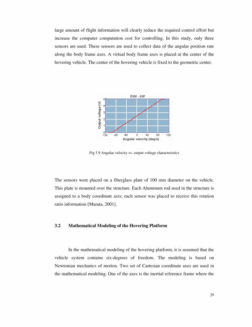
29

large amount of flight information will clearly reduce the required control effort but

increase the computer computation cost for controlling. In this study, only three

sensors are used. These sensors are used to collect data of the angular position rate

along the body frame axes. A virtual body frame axes is placed at the center of the

hovering vehicle. The center of the hovering vehicle is fixed to the geometric center.

Fig 3.9 Angular velocity vs. output voltage characteristics

The sensors were placed on a fiberglass plate of 100 mm diameter on the vehicle.

This plate is mounted over the structure. Each Aluminum rod used in the structure is

assigned to a body coordinate axis; each sensor was placed to receive this rotation

ratio information [Murata, 2001].

3.2 Mathematical Modeling of the Hovering Platform

In the mathematical modeling of the hovering platform, it is assumed that the

vehicle system contains six-degrees of freedom. The modeling is based on

Newtonian mechanics of motion. Two set of Cartesian coordinate axes are used in

the mathematical modeling. One of the axes is the inertial reference frame where the

30

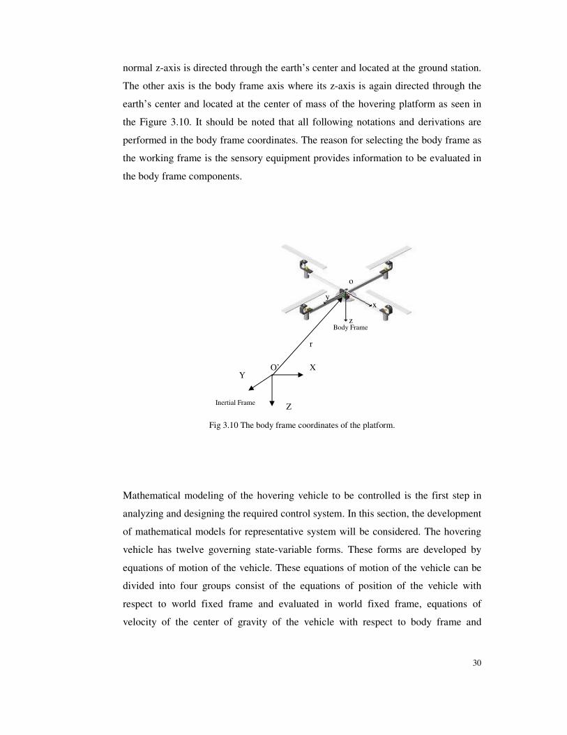
normal z-axis is directed through the earth’s center and located at the ground station.

The other axis is the body frame axis where its z-axis is again directed through the

earth’s center and located at the center of mass of the hovering platform as seen in

the Figure 3.10. It should be noted that all following notations and derivations are

performed in the body frame coordinates. The reason for selecting the body frame as

the working frame is the sensory equipment provides information to be evaluated in

the body frame components.

Fig 3.10 The body frame coordinates of the platform.

Mathematical modeling of the hovering vehicle to be controlled is the first step in

analyzing and designing the required control system. In this section, the development

of mathematical models for representative system will be considered. The hovering

vehicle has twelve governing state-variable forms. These forms are developed by

equations of motion of the vehicle. These equations of motion of the vehicle can be

divided into four groups consist of the equations of position of the vehicle with

respect to world fixed frame and evaluated in world fixed frame, equations of

velocity of the center of gravity of the vehicle with respect to body frame and

z

x y

X

Z

Y O’

o

r

Inertial Frame

Body Frame

31

evaluated in body frame, equations of motion of the angular velocity of the vehicle

about its principal axes with respect to body frame and evaluated in body frame and

the equations of angles of the vehicle with respect to body frame and evaluated in

body frame. Each group of equations represents the motion of the hovering vehicle

partially. Each group of equations consists of three state-variables that are the ( )kji��

,,

components of the related vectors namely the position, velocity, angular velocity and

the body frame angle. These differential equations can be expressed as a set of

simultaneous first-order differential equations and solved by a computer package

program. The solution of the state variables will be used in the controller design.

The first set of variables is the components of the position vector of the center of

mass of the vehicle with respect to world fixed inertial frame. The components of

position vector can be evaluated in terms of absolute velocity of the center of mass of

the platform with respect to world fixed inertial frame. The position vector of the

center of mass of the vehicle with respect to the inertial frame is defined as;

kzjyixr�� ++= (3.1)

which gives the absolute velocity vector as;

kzjyixr��

��

�� ++= (3.2)

Note that, in the equations “ �” represents the derivative with respect to time and yx ��,

and z� are the components of velocity along the x, y, z directions, respectively. The

components of the absolute velocity term in inertial frame can be written in body

frame with the form;

��

�

�

��

�

�

=��

�

�

��

�

�

w

v

u

R

z

y

x

IB

�

�

�

(3.3)

32

with u , v and w being the absolute velocity components in the body frame. BIR is

the rotation matrix from inertial frame to body frame components and can be given

by;

��

�

�

��

�

�

+−++−

−=

φθψφθψφψφφθψφθψφθψφψφφθψ

θψθψθ

coscossincossincossinsinsincossincossincossinsinsincoscossincossinsincos

sinsincoscoscos

BIR (3.4)

Note that, BIR has the following property

TBIBIIB RRR == −1

(3.5)

In the above equations, the angles represent the rotations around the three axes that

is;

φ : Roll Angle (phi) = Rotation about the body fixed x axis

θ : Pitch Angle (tetha) = Rotation about the body fixed y axis

ψ : Yaw Angle (psi) = Rotation about the body fixed z axis

The order of these angles is →→→ Θ ψφ toto . Using these definitions together

with equations (3.3), (3.4) and (3.5), it is possible to write;

( ) ( ) ( )wvux ψφφθψψφφθψψθ sinsincossincossincossinsincoscoscos ++−+=� (3.6)

( ) ( ) ( )wvuy ψφθψφψφθψφψθ sincossincossinsinsinsincoscossincos +−+++=� (3.7)

( ) ( ) ( )wvuz φθφθθ coscossincossin ++−=� (3.8)

In the derivations, vertical altitude can be expressed as zh −= where;

( ) ( ) ( )wvuh φθφθθ coscossincossin −−=� (3.9)

From the equations given in (3.6)-(3.8), it can be seen that the first set of variables

( )zyx ,, to be solved is the velocity component rates of the hovering platform.

33

Evaluating these variables give the coordinates of the hovering platform ( )zyx ,,

with respect to the inertial frame.

The second set of variables ( )wvu ,, are the velocity components of the hovering

platform with respect to inertial frame expressed in body frame. The difference

between the first set of variables and the second set of variables is the coordinate

axes of resolution. Three gyroscopes were used to sense the rotation rates about their

related axis on the body frame axes. Sensor data gives these velocity components

directly.

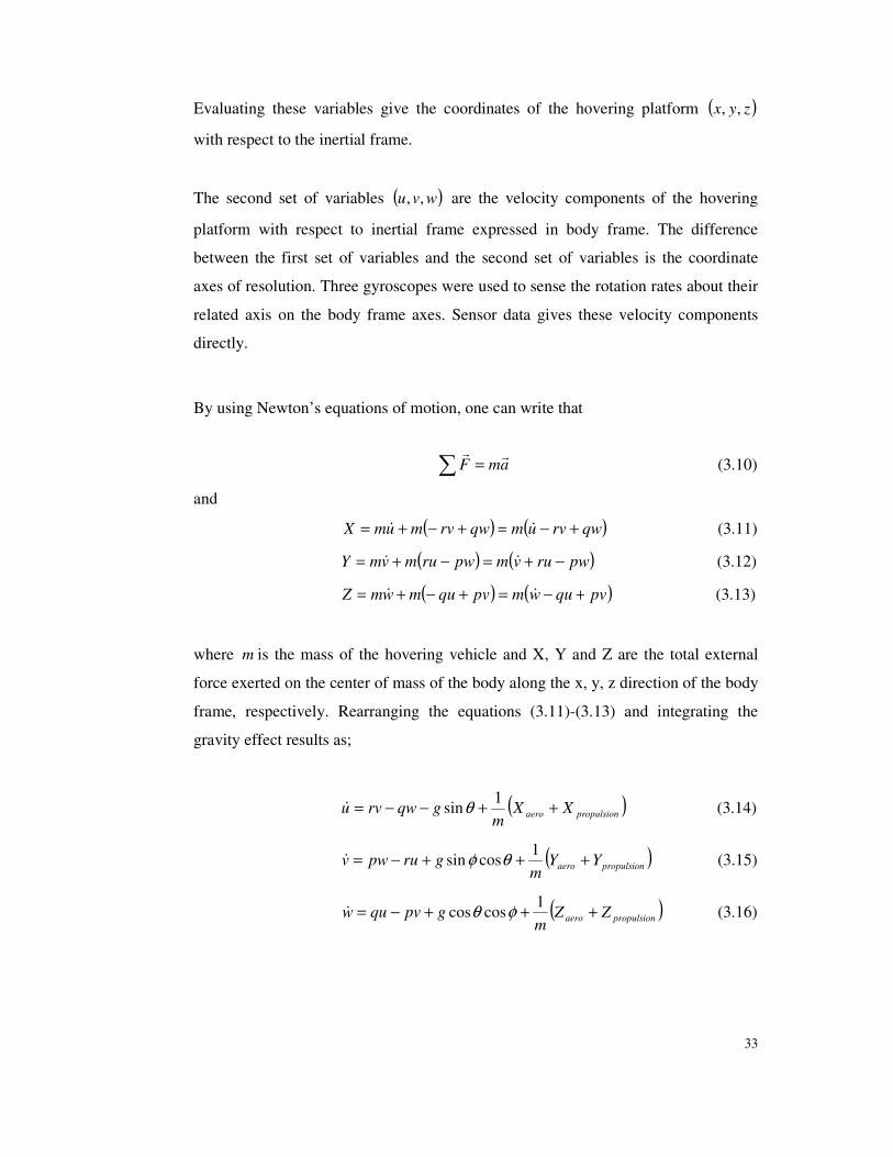
By using Newton’s equations of motion, one can write that

� = amF��

(3.10)

and

( ) ( )qwrvumqwrvmumX +−=+−+= �� (3.11)

( ) ( )pwruvmpwrumvmY −+=−+= �� (3.12)

( ) ( )pvquwmpvqumwmZ +−=+−+= �� (3.13)

where m is the mass of the hovering vehicle and X, Y and Z are the total external

force exerted on the center of mass of the body along the x, y, z direction of the body

frame, respectively. Rearranging the equations (3.11)-(3.13) and integrating the

gravity effect results as;

( )propulsionaero XXm

gqwrvu ++−−= 1sinθ� (3.14)

( )propulsionaero YYm

grupwv +++−= 1cossin θφ� (3.15)

( )propulsionaero ZZm

gpvquw +++−= 1coscos φθ� (3.16)

34

with note that, in the above equations, the terms p, q, r are the rate of rotation about

the x, y, z axis of the body fixed frame.

The third set of variables is the angular velocity components (p, q, r) of the hovering

platform with respect to inertial frame expressed in body frame. Sensor data

measures these velocity components in a noisy form.

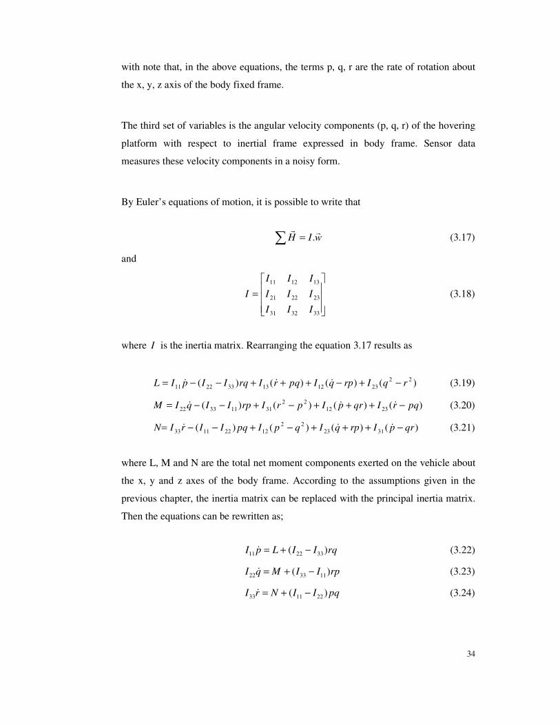
By Euler’s equations of motion, it is possible to write that

wIH��

.=� (3.17)

and

��

��

�

=

333231

232221

131211

III

III

III

I (3.18)

where I is the inertia matrix. Rearranging the equation 3.17 results as

)()()()( 22231213332211 rqIrpqIpqrIrqIIpIL −+−+++−−= �� (3.19)

)()()()( 231222

31113322 pqrIqrpIprIrpIIqIM −+++−+−−= �� (3.20)

)()()()( 312322

12221133 qrpIrpqIqpIpqIIrIN −+++−+−−= �� (3.21)

where L, M and N are the total net moment components exerted on the vehicle about

the x, y and z axes of the body frame. According to the assumptions given in the

previous chapter, the inertia matrix can be replaced with the principal inertia matrix.

Then the equations can be rewritten as;

rqIILpI )( 332211 −+=� (3.22)

rpIIMqI )( 113322 −+=� (3.23)

pqIINrI )( 221133 −+=� (3.24)

35

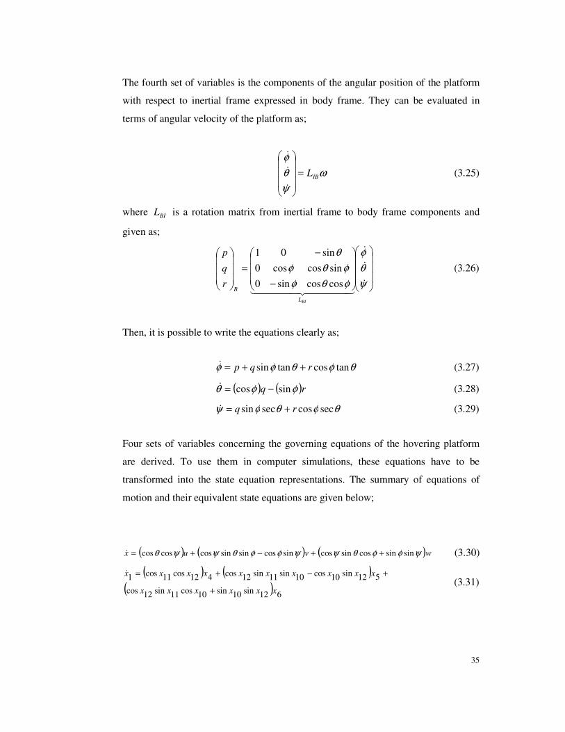
The fourth set of variables is the components of the angular position of the platform

with respect to inertial frame expressed in body frame. They can be evaluated in

terms of angular velocity of the platform as;

ωψθφ

IBL=��

�

�

��

�

�

�

�

�

(3.25)

where BIL is a rotation matrix from inertial frame to body frame components and

given as;

��

�

�

��

�

�

��

�

�

��

�

�

−

−=

��

�

�

��

�

�

ψθφ

φθφφθφ

θ

�

�

�

�� BIL

Br

q

p

coscossin0sincoscos0

sin01 (3.26)

Then, it is possible to write the equations clearly as;

θφθφφ tancostansin rqp ++=� (3.27)

( ) ( )rq φφθ sincos −=� (3.28)

θφθφψ seccossecsin rq +=� (3.29)

Four sets of variables concerning the governing equations of the hovering platform

are derived. To use them in computer simulations, these equations have to be

transformed into the state equation representations. The summary of equations of

motion and their equivalent state equations are given below;

( ) ( ) ( )wvux ψφφθψψφφθψψθ sinsincossincossincossinsincoscoscos ++−+=� (3.30)

( ) ( )( ) 612sin10sin10cos11sin12cos

512sin10cos10sin11sin12cos412cos11cos1

xxxxxx

xxxxxxxxxx

+

+−+=� (3.31)

36

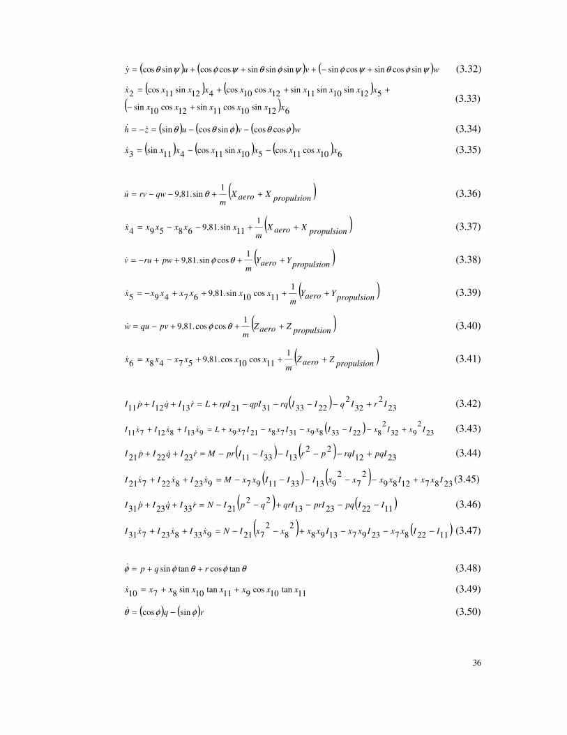
( ) ( ) ( )wvuy ψφθψφψφθψφψθ sincossincossinsinsinsincoscossincos +−+++=� (3.32) ( ) ( )

( ) 612sin10cos11sin12cos10sin

512sin10sin11sin12cos10cos412sin11cos2

xxxxxx

xxxxxxxxxx

+−

+++=� (3.33)

( ) ( ) ( )wvuzh φθφθθ coscossincossin −−=−= �� (3.34)

( ) ( ) ( ) 610cos11cos510sin11cos411sin3 xxxxxxxxx −−=� (3.35)

( )propulsionXaeroXm

qwrvu ++−−=1

sin.81,9 θ� (3.36)

( )propulsionXaeroXm

xxxxxx ++−−=1

11sin.81,968594� (3.37)

( )propulsionYaeroYm

pwruv ++++−=1

cossin.81,9 θφ� (3.38)

( )propulsionYaeroYm

xxxxxxx ++++−=1

11cos10sin.81,967495� (3.39)

( )propulsionZaeroZm

pvquw +++−=1

coscos.81,9 θφ� (3.40)

( )propulsionZaeroZm

xxxxxxx +++−=1

11cos10cos.81,957486� (3.41)

( ) 232

322

22333121131211 IrIqIIrqqpIrpILrIqIpI +−−−−+=++ �� (3.42)

( ) 232

9322

822338931782179913812711 IxIxIIxxIxxIxxLxIxIxI +−−−−+=++ �� (3.43)

( ) ( ) 231222

133311232221 pqIrqIprIIIprMrIqIpI +−−−−−=++ �� (3.44)

( ) ( ) 238712892

72

913331197923822721 IxxIxxxxIIIxxMxIxIxI +−−−−−=++ �� (3.45)

( ) ( )1122231322

21332331 IIpqprIqrIqpINrIqIpI −−−+−−=++ �� (3.46)

( ) ( )112287239713982

82

721933823731 IIxxIxxIxxxxINxIxIxI −−−+−−=++ �� (3.47)

θφθφφ tancostansin rqp ++=� (3.48)

11tan10cos911tan10sin8710 xxxxxxxx ++=� (3.49)

( ) ( )rq φφθ sincos −=� (3.50)

37

( ) ( ) 910sin810cos11 xxxxx −=� (3.51)

θφθφψ seccossecsin rq +=� (3.52)

11sec10cos911sec10sin812 xxxxxxx +=� (3.53)

In the above equations, the predetermined assumptions are applied. The mass

moment of inertia is in 2.mkg and found to be in AutoCad 2002 Mechanical Desktop

and evaluated in the body frame as;

��

��

�

=−

−

−

3

3

3

102.3000106.1000106.1

xx

x

I

It is assumed that there is no x or y directional forces exerted on the vehicle, except

some small disturbances occurred by the irregularities during manufacturing. The z

directional force is just the sum of the thrusts generated by each propeller.

�=

=

≅≅

4

1iiz

y

x

FF

0F0F

(3.54)

The given moment forces are the generated moments in the x and y axes. In this

study, the 1st and 3rd propellers rotate in clockwise and the other 2nd and 4th ones

rotates in the counter clockwise. All four DC motors generate axial moments. At the

mean while, each motor generates counter torques. These torques cannot be

eliminated.

( )( )

( )4321z

42y

31x

FFFF-CM

FFM

FFM

+−+=

−=−=

l

l

(3.55)

38

In the above equations, l is the bird eye moment arm length between the center of

mass of the vehicle and the propeller’s geometrical center. iF represents the thrust

force exerted by each power unit/propeller. All iF is in the vertical axis. iF values of

each motor are calculated for each power unit using the experiments mentioned

before. The resultant z-axis moment, zM , value can be estimated as given in the

equation (3.31). This estimation neglects the effect of DC motor modeling [Altu� E.,

Ostrowski J.P., Mahony R., 2003]. The coefficient C is a small number and

experimentally deduced. For the C value, 0.1, 0.01 and 0.001 values are tested in real

time experiments. It is decided to use C=0.1 at the end of these tests.

39

CHAPTER IV

CONTROLLER DESIGN

In this study, the goal is to stabilize the hovering vehicle in the air, with the

given inertial measurement units. To stabilize the vehicle, a control system has to be

considered. Without a control effort, irregularities and the working conditions of the

manufactured vehicle will cause unstable motions. Linear quadratic regulator (LQR)

controller is selected to stabilize the vehicle. On the other hand, LQR can only be

applied to a full rank observable system. To apply the LQR, the equations of motion

of the vehicle have to be represented in state-space form. A measurement noise

problem is detected and a second order transfer function with a low-pass filter is used

to solve the noise elimination problem. The following sections detail the theoretical

and experimental efforts and their comparison on the hovering vehicle.

4.1 Linear quadratic regulator

Linear quadratic regulator is one of the most effective and widely used

modern control technique, partially due to the ease of implementation and its

optimality to linear time invariant systems. It is an optimal and robust technique for

Multi Input Multi Output (MIMO) control. This method allows finding the optimal

control feedback coefficients that result in some balance between system errors and

control effort. This method simply drives the outputs to zero during the process.

40

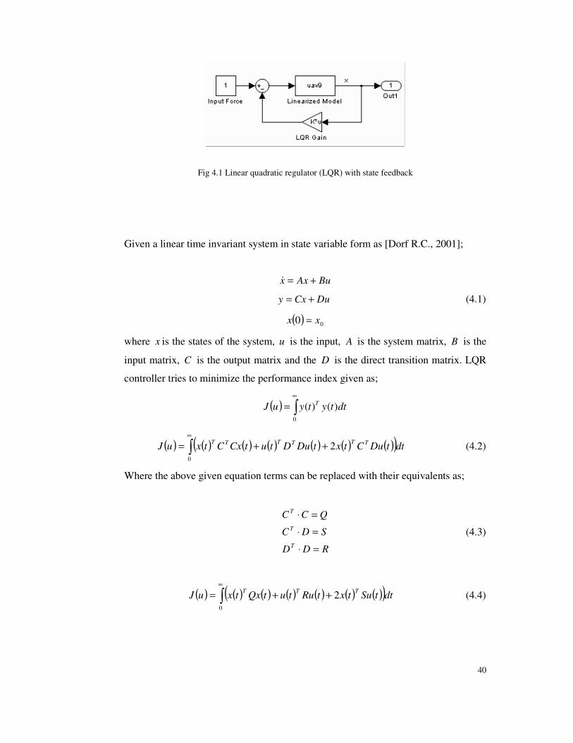
Fig 4.1 Linear quadratic regulator (LQR) with state feedback

Given a linear time invariant system in state variable form as [Dorf R.C., 2001];

BuAxx +=�

DuCxy += (4.1)

( ) 00 xx =

where x is the states of the system, u is the input, A is the system matrix, B is the

input matrix, C is the output matrix and the D is the direct transition matrix. LQR

controller tries to minimize the performance index given as;

( ) �∞

=0

)()( dttytyuJ T

( ) ( ) ( ) ( ) ( ) ( ) ( )( )�∞

++=0

2 dttDuCtxtDuDtutCxCtxuJ TTTTTT (4.2)

Where the above given equation terms can be replaced with their equivalents as;

RDD

SDC

QCC

T

T

T

=⋅

=⋅

=⋅

(4.3)

( ) ( ) ( ) ( ) ( ) ( ) ( )( )�∞

++=0

2 dttSutxtRututQxtxuJ TTT (4.4)

41

The linear solution that minimizes this index is given by some linear function of

states;

Kxu −= (4.5)

and the feedback gain is given as;

( )TT SPBRK +−= −1 (4.6)

Linear quadratic regulator solves also a Ricatti equation given as;

( ) ( ) 01 =+++−+ − QSPBRSPBPAPA TTT (4.7)

where P is the stabilizing solution to the Ricatti equation [Lewis F.L., 1999].

( ) ( ) 000

PxxdttytyJ TT == �∞

(4.8)

Linear quadratic regulator assumes that all the states are measurable and the system

is observable and linear. Non-linear equations of motion have to be linearized to use

the Linear quadratic regulator controller. In the above equation (4.3), Q is the state

control matrix and it is important when defining which states are more important and

which are less important. It means that, larger values of Q generally results in the

poles of the closed loop system being left in the s-plane so that the states decay faster

to zero. On the other hand, R is the performance index matrix also referred as the

cost of inputs. Experiments are used to get the fastest response depending on

different Q and R matrices [Hespanha J. P., 2004].

4.2 Linearization of the equations

When the equations of motion of the hovering vehicle are considered, it is

seen that the governing motion equations are non-linear. These equations have to be

linearized about the stable hovering conditions,

[ ]0 00 0000000000 =x , to represent the system in state-space

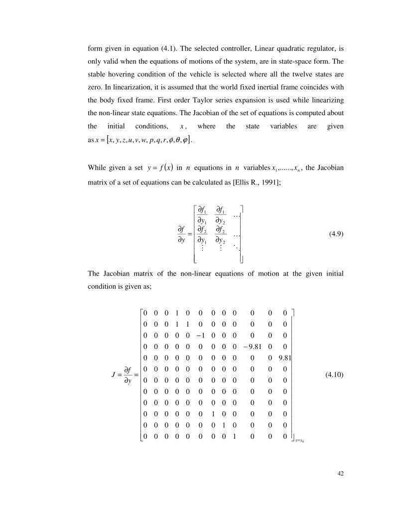
42

form given in equation (4.1). The selected controller, Linear quadratic regulator, is

only valid when the equations of motions of the system, are in state-space form. The

stable hovering condition of the vehicle is selected where all the twelve states are

zero. In linearization, it is assumed that the world fixed inertial frame coincides with

the body fixed frame. First order Taylor series expansion is used while linearizing

the non-linear state equations. The Jacobian of the set of equations is computed about

the initial conditions, x , where the state variables are given

as [ ]ϕθφ ,,,,,,,,,,, rqpwvuzyxx = .

While given a set ( )xfy = in n equations in n variables nxx ,......,1 , the Jacobian

matrix of a set of equations can be calculated as [Ellis R., 1991];

��

��

�

∂∂

∂∂

∂∂

∂∂

=∂∂

��

2

2

1

2

2

1

1

1

yf

yf

yf

yf

yf

(4.9)

The Jacobian matrix of the non-linear equations of motion at the given initial

condition is given as;

000010000000000001000000000000100000000000000000000000000000000000000000000000000000081.9000000000000081.9000000000000000100000000000011000000000001000

xx

yf

J

=��

��

�

−−

=∂∂= (4.10)

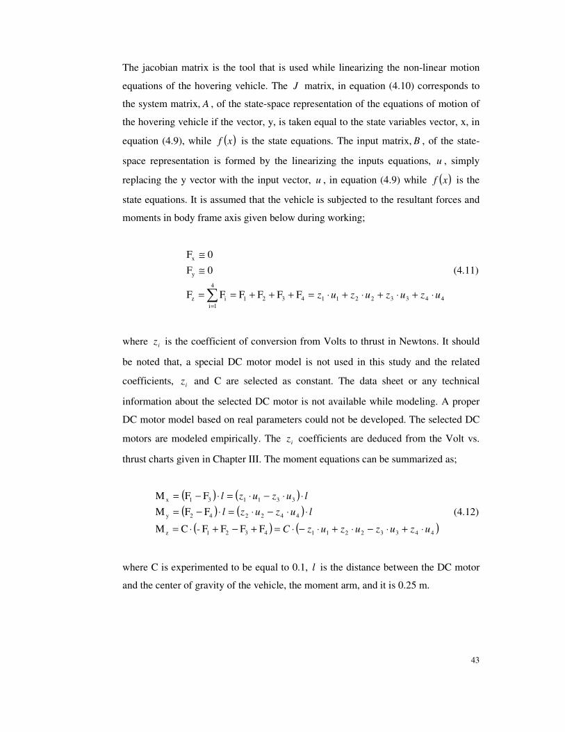
43

The jacobian matrix is the tool that is used while linearizing the non-linear motion

equations of the hovering vehicle. The J matrix, in equation (4.10) corresponds to

the system matrix, A , of the state-space representation of the equations of motion of

the hovering vehicle if the vector, y, is taken equal to the state variables vector, x, in

equation (4.9), while ( )xf is the state equations. The input matrix, B , of the state-

space representation is formed by the linearizing the inputs equations, u , simply

replacing the y vector with the input vector, u , in equation (4.9) while ( )xf is the

state equations. It is assumed that the vehicle is subjected to the resultant forces and

moments in body frame axis given below during working;

443322114321

4

1iiz

y

x

FFFFFF

0F0F

uzuzuzuz ⋅+⋅+⋅+⋅=+++==

≅≅

�=

(4.11)

where iz is the coefficient of conversion from Volts to thrust in Newtons. It should

be noted that, a special DC motor model is not used in this study and the related

coefficients, iz and C are selected as constant. The data sheet or any technical

information about the selected DC motor is not available while modeling. A proper

DC motor model based on real parameters could not be developed. The selected DC

motors are modeled empirically. The iz coefficients are deduced from the Volt vs.

thrust charts given in Chapter III. The moment equations can be summarized as;

( ) ( )( ) ( )

( ) ( )443322114321z

442242y

331131x

FFFF-CM

FFM

FFM

uzuzuzuzC

luzuzl

luzuzl

⋅+⋅−⋅+⋅−⋅=+−+⋅=

⋅⋅−⋅=⋅−=⋅⋅−⋅=⋅−=

(4.12)

where C is experimented to be equal to 0.1, l is the distance between the DC motor

and the center of gravity of the vehicle, the moment arm, and it is 0.25 m.

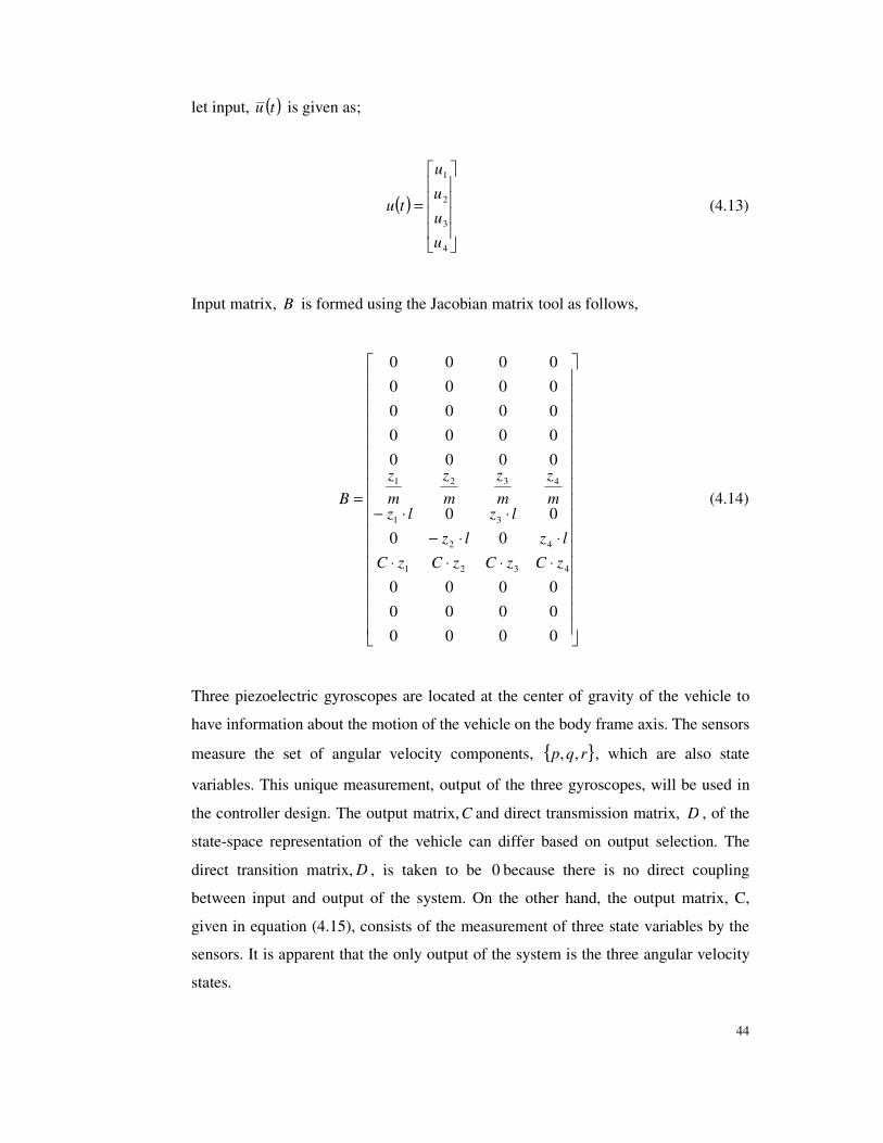
44

let input, ( )tu is given as;

( )��

��

�

=

4

3

2

1

u

u

u

u

tu (4.13)

Input matrix, B is formed using the Jacobian matrix tool as follows,

��

��

�

⋅⋅⋅⋅⋅⋅−

⋅⋅−=

000000000000

0000

00000000000000000000

4321

42

31

4321

zCzCzCzC

lzlz

lzlzmz

mz

mz

mz

B (4.14)

Three piezoelectric gyroscopes are located at the center of gravity of the vehicle to

have information about the motion of the vehicle on the body frame axis. The sensors

measure the set of angular velocity components, { }rqp ,, , which are also state

variables. This unique measurement, output of the three gyroscopes, will be used in

the controller design. The output matrix,C and direct transmission matrix, D , of the

state-space representation of the vehicle can differ based on output selection. The

direct transition matrix, D , is taken to be 0 because there is no direct coupling

between input and output of the system. On the other hand, the output matrix, C,

given in equation (4.15), consists of the measurement of three state variables by the

sensors. It is apparent that the only output of the system is the three angular velocity

states.

45

��

��

�

=

000000000000000000000000000000000000000100000000000010000000000001000000000000000000000000000000000000000000000000000000000000000000000000000000

C (4.15)

Selecting the output matrix, C , given in equation (4.15), the output of the system

turns out to be as;

��

��

�

=��

��

�

=+=r

q

p

x

x

x

DuCxy

9

8

7

(4.16)

4.3 Controllability

A system is completely controllable if there exists an unconstrained control

( )tu that can transfer any initial state ( )0tx to any other desired location ( )tx in a

finite time, Ttt ≤≤0 [D. Goshen-Meskin, 1992]. When a nonlinear system is

linearized about an initial point, ( )0x , there exits a set of equations given in equation

(4.1). The controllability of a linear system can be stated according to the rank of

controllability matrix, Co , given in equation (4.17). The rank of the controllability

matrix,Co , determines the number of controllable states in the system. In this

46

application, the number of states, n , and the controllability matrix is full rank. It

means that the system is completely state controllable.

[ ]BA.....BAABBCo )(n-12= (4.17)

where, A is the system matrix, B is the input matrix and n is the number of states.

Co matrix is given in Appendix II.

4.4 Observability

A system is said to be observable at time 0t if its state vector at time 0t , ( )0tx ,

can be determined from the output function [ ]10 ,tty where 1t , 10 tt ≤ is some finite time.

If this is true for all 0t and ( )0tx the system is said to be completely observable [D.

Goshen-Meskin, 1992]. For a given linear time invariant system, state space

representation is given in equation (4.1).

For a linear time invariant system to be completely state observable, the observability

matrix given in equation (4.18) must have a rank of n . Otherwise, the rank of

observability matrix indicates the number of states that are observable.

��

��

�

=

1

2

n-CA

.

.

CA

CA

C

O (4.18)

where, A is the system matrix, C is the output matrix and n is the number of states.

O matrix is given in Appendix II.

When the twelve non-linear state-variable equations of motion of the hovering

vehicle are linearized about the stable hovering conditions, 0x , and the state

47

equations are represented in state-space form, the state-space representation of the

equations of motions of the vehicle can be used to calculate the rank of the

observability matrix of the plant. The rank of the observability matrix of the hovering

platform dealt in this project is computed to be three (3). The rank of the

observability matrix is a measure of the number of states that are observed /

monitored. The hovering vehicle system is unobservable because the observability

matrix is not full rank. It is apparent that only the three states { }rqp ,, can be

observed by the three gyros. The rest of nine states could not be monitored.

If a state-variable is measured and fed back for use in control computations, the

system is called closed-loop or feedback control [Franklin G. F., 2002]. For a given

plant and state equations;

BuAxx +=� (4.19)

the objective is to find a state feedback control law as;

Kxu −= (4.20)

The selected controller for this application is the Linear quadratic regulator and its

feedback gain K is computed as given in equation (4.6). The gain matrix, K , is a

4x12 dimensional matrix. Computationally, such a gain, K , is possible to find for

twelve state-variables. To control and stabilize the overall plant with proper feedback

signal u , the 12x1 state vector, x has to be known, too. The state vector, x , has to

be numerically calculated as the feedback gain, K . These numerical values are the

sensor measurements of the system. Unfortunatelly, because there are only three

gyroscopic sensors, it is not possible to observe the twelve states as stated before.

Therefore, there are some numerically undetermined missing/unknown states-

variables in the hovering platform state vector, x .

When it is not possible to observe all the system states-variables by some inertial

measurement units or estimate somehow, an applicable Linear quadratic regulator

control signal,u , can not be used in the linear system as a controller. To able to use

48

the Linear quadratic regulator, a state estimator to observe all the twelve states will

be needed or controlling of observable states will be considered. A linear state

estimator cannot be used because the states are unobservable and the use of a non-

linear state estimator is not proposed to use in this study

On the other hand, the controlling of the observed states can be applied to the system

while considering the Linear quadratic regulator. By controlling of the observed

states, it is assumed that the system does not lose its original governing twelve states

but the Linear quadratic regulator feedback gain, K is applied to the observed states

rather than the total number of states. In this case, a 4x3 gain matrix K is

reconstructed for the observed states by the observed state-variable equations. If the

Linear quadratic regulator feedback gain coefficient is only computed considering

the observed states, the controlling and stabilizing of the observed states will be

possible. Only the observed rotational states-variables, p,q,r, are possible to control

[Chen M., Huzmezan M., 2003]. At the initial conditions, straightforward

mathematical relationships can be derived between the rotational rates and the

rotation angles. At the end, it should be clarified that, in this study, only the

controlling of the six states of rotation is achieved but the position and velocity

control of the hovering vehicle is not possible to control.

4.5 Noise Filtering

The three sensors provide information about the angular rotation rates of the

hovering vehicle. When the sensor measurements are corrupted by random

variations, it is possible to say that they are affected by noise. Since the standard

deviation is a measure of spread in data distribution, these random variations can be

characterized by the standard deviation of measured signals. It is possible to say that

when the standard deviation gets larger, the noise effect increases. [Opphenheim A.

V. 1999]

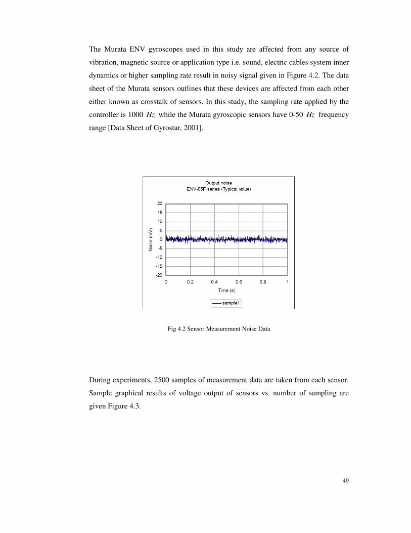
49

The Murata ENV gyroscopes used in this study are affected from any source of

vibration, magnetic source or application type i.e. sound, electric cables system inner

dynamics or higher sampling rate result in noisy signal given in Figure 4.2. The data

sheet of the Murata sensors outlines that these devices are affected from each other

either known as crosstalk of sensors. In this study, the sampling rate applied by the

controller is 1000 Hz while the Murata gyroscopic sensors have 0-50 Hz frequency

range [Data Sheet of Gyrostar, 2001].

Fig 4.2 Sensor Measurement Noise Data

During experiments, 2500 samples of measurement data are taken from each sensor.

Sample graphical results of voltage output of sensors vs. number of sampling are

given Figure 4.3.

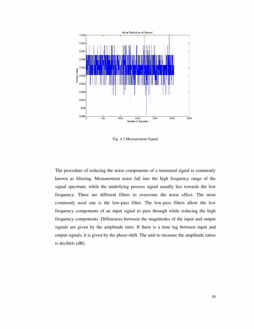
50

Fig. 4.3 Measurement Signal

The procedure of reducing the noise components of a measured signal is commonly

known as filtering. Measurement noise fall into the high frequency range of the

signal spectrum, while the underlying process signal usually lies towards the low

frequency. There are different filters to overcome the noise effect. The most

commonly used one is the low-pass filter. The low-pass filters allow the low

frequency components of an input signal to pass through while reducing the high

frequency components. Differences between the magnitudes of the input and output

signals are given by the amplitude ratio. If there is a time lag between input and

output signals, it is given by the phase-shift. The unit to measure the amplitude ratios

is decibels (dB).

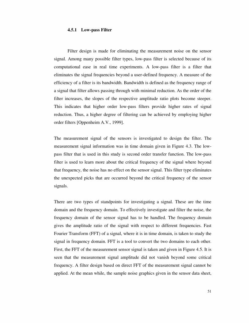
51

4.5.1 Low-pass Filter

Filter design is made for eliminating the measurement noise on the sensor

signal. Among many possible filter types, low-pass filter is selected because of its

computational ease in real time experiments. A low-pass filter is a filter that

eliminates the signal frequencies beyond a user-defined frequency. A measure of the

efficiency of a filter is its bandwidth. Bandwidth is defined as the frequency range of

a signal that filter allows passing through with minimal reduction. As the order of the

filter increases, the slopes of the respective amplitude ratio plots become steeper.

This indicates that higher order low-pass filters provide higher rates of signal

reduction. Thus, a higher degree of filtering can be achieved by employing higher

order filters [Oppenheim A.V., 1999].

The measurement signal of the sensors is investigated to design the filter. The

measurement signal information was in time domain given in Figure 4.3. The low-

pass filter that is used in this study is second order transfer function. The low-pass

filter is used to learn more about the critical frequency of the signal where beyond

that frequency, the noise has no effect on the sensor signal. This filter type eliminates

the unexpected picks that are occurred beyond the critical frequency of the sensor

signals.

There are two types of standpoints for investigating a signal. These are the time

domain and the frequency domain. To effectively investigate and filter the noise, the

frequency domain of the sensor signal has to be handled. The frequency domain

gives the amplitude ratio of the signal with respect to different frequencies. Fast

Fourier Transform (FFT) of a signal, where it is in time domain, is taken to study the

signal in frequency domain. FFT is a tool to convert the two domains to each other.

First, the FFT of the measurement sensor signal is taken and given in Figure 4.5. It is

seen that the measurement signal amplitude did not vanish beyond some critical

frequency. A filter design based on direct FFT of the measurement signal cannot be

applied. At the mean while, the sample noise graphics given in the sensor data sheet,

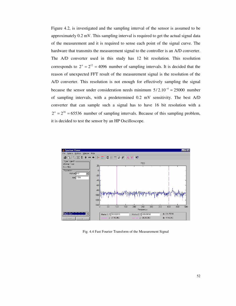
52

Figure 4.2, is investigated and the sampling interval of the sensor is assumed to be

approximately 0.2 mV. This sampling interval is required to get the actual signal data

of the measurement and it is required to sense each point of the signal curve. The

hardware that transmits the measurement signal to the controller is an A/D converter.

The A/D converter used in this study has 12 bit resolution. This resolution

corresponds to 409622 12 ==n number of sampling intervals. It is decided that the

reason of unexpected FFT result of the measurement signal is the resolution of the

A/D converter. This resolution is not enough for effectively sampling the signal

because the sensor under consideration needs minimum 2500010.2/5 4 =− number

of sampling intervals, with a predetermined 0.2 mV sensitivity. The best A/D

converter that can sample such a signal has to have 16 bit resolution with a

6553622 16 ==n number of sampling intervals. Because of this sampling problem,

it is decided to test the sensor by an HP Oscilloscope.

Fig. 4.4 Fast Fourier Transform of the Measurement Signal

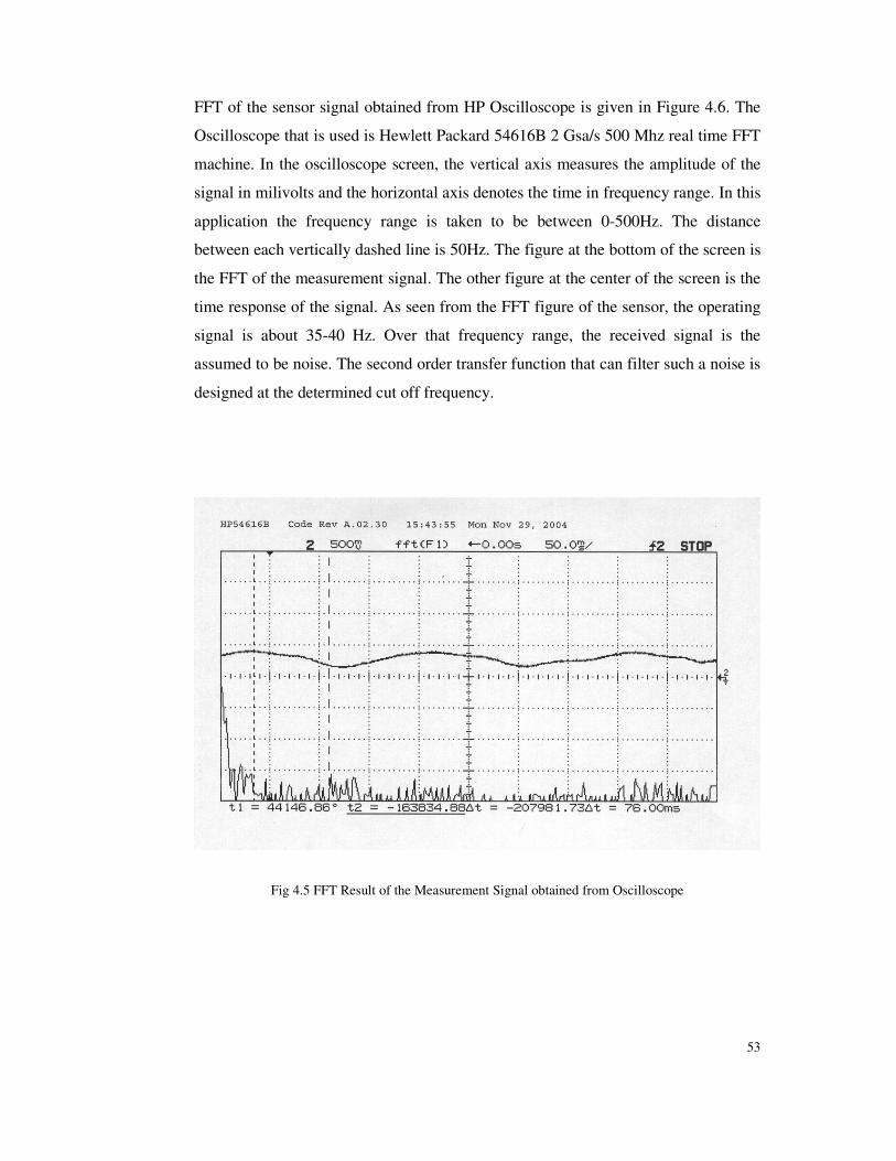
53

FFT of the sensor signal obtained from HP Oscilloscope is given in Figure 4.6. The

Oscilloscope that is used is Hewlett Packard 54616B 2 Gsa/s 500 Mhz real time FFT

machine. In the oscilloscope screen, the vertical axis measures the amplitude of the

signal in milivolts and the horizontal axis denotes the time in frequency range. In this

application the frequency range is taken to be between 0-500Hz. The distance

between each vertically dashed line is 50Hz. The figure at the bottom of the screen is

the FFT of the measurement signal. The other figure at the center of the screen is the

time response of the signal. As seen from the FFT figure of the sensor, the operating

signal is about 35-40 Hz. Over that frequency range, the received signal is the

assumed to be noise. The second order transfer function that can filter such a noise is

designed at the determined cut off frequency.

Fig 4.5 FFT Result of the Measurement Signal obtained from Oscilloscope

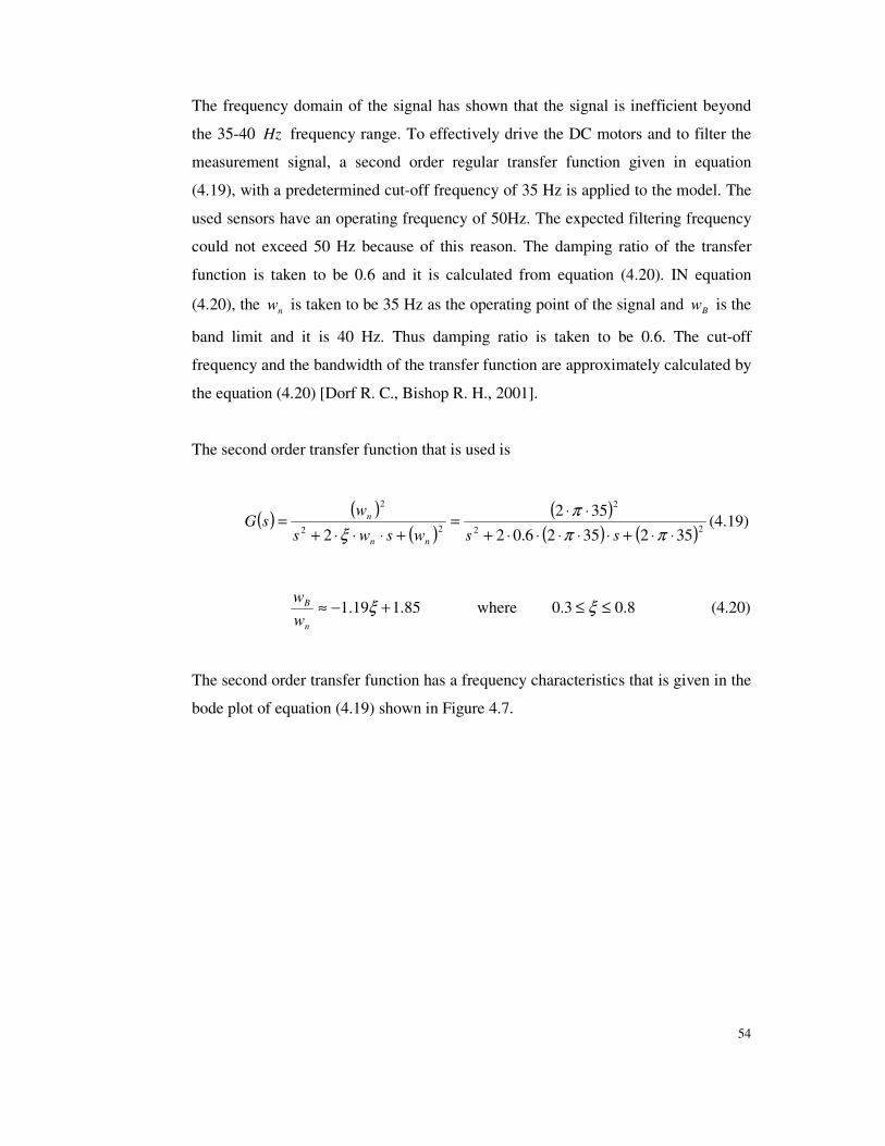
54

The frequency domain of the signal has shown that the signal is inefficient beyond

the 35-40 Hz frequency range. To effectively drive the DC motors and to filter the

measurement signal, a second order regular transfer function given in equation

(4.19), with a predetermined cut-off frequency of 35 Hz is applied to the model. The

used sensors have an operating frequency of 50Hz. The expected filtering frequency

could not exceed 50 Hz because of this reason. The damping ratio of the transfer

function is taken to be 0.6 and it is calculated from equation (4.20). IN equation

(4.20), the nw is taken to be 35 Hz as the operating point of the signal and Bw is the

band limit and it is 40 Hz. Thus damping ratio is taken to be 0.6. The cut-off

frequency and the bandwidth of the transfer function are approximately calculated by

the equation (4.20) [Dorf R. C., Bishop R. H., 2001].

The second order transfer function that is used is

( ) ( )( )

( )( ) ( )22

2

22

2

3523526.02352

2 ⋅⋅+⋅⋅⋅⋅⋅+⋅⋅=

+⋅⋅⋅+=

πππ

ξ sswsws

wsG

nn

n (4.19)

8.03.0 where 85.119.1 ≤≤+−≈ ξξn

B

ww

(4.20)

The second order transfer function has a frequency characteristics that is given in the

bode plot of equation (4.19) shown in Figure 4.7.

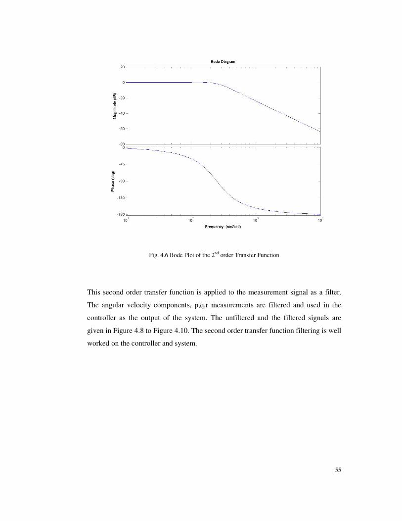
55

Fig. 4.6 Bode Plot of the 2nd order Transfer Function

This second order transfer function is applied to the measurement signal as a filter.

The angular velocity components, p,q,r measurements are filtered and used in the

controller as the output of the system. The unfiltered and the filtered signals are

given in Figure 4.8 to Figure 4.10. The second order transfer function filtering is well

worked on the controller and system.

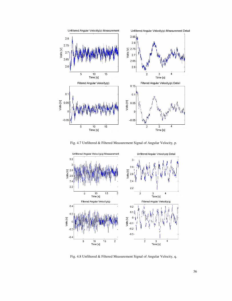
56

Fig. 4.7 Unfiltered & Filtered Measurement Signal of Angular Velocity, p.

Fig. 4.8 Unfiltered & Filtered Measurement Signal of Angular Velocity, q.

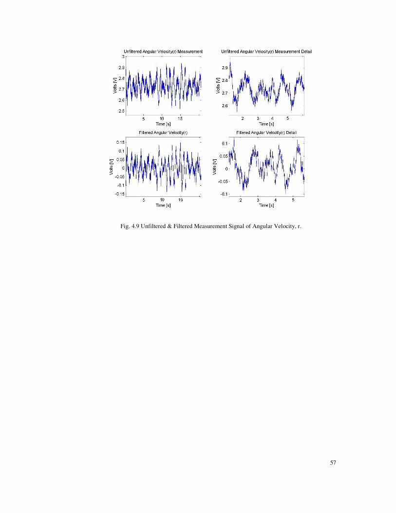
57

Fig. 4.9 Unfiltered & Filtered Measurement Signal of Angular Velocity, r.

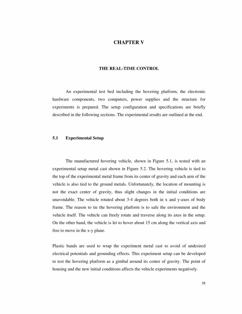
58

CHAPTER V

THE REAL-TIME CONTROL

An experimental test bed including the hovering platform, the electronic

hardware components, two computers, power supplies and the structure for

experiments is prepared. The setup configuration and specifications are briefly

described in the following sections. The experimental results are outlined at the end.

5.1 Experimental Setup

The manufactured hovering vehicle, shown in Figure 5.1, is tested with an

experimental setup metal cast shown in Figure 5.2. The hovering vehicle is tied to

the top of the experimental metal frame from its center of gravity and each arm of the

vehicle is also tied to the ground metals. Unfortunately, the location of mounting is

not the exact center of gravity, thus slight changes in the initial conditions are

unavoidable. The vehicle rotated about 3-4 degrees both in x and y-axes of body

frame. The reason to tie the hovering platform is to safe the environment and the

vehicle itself. The vehicle can freely rotate and traverse along its axes in the setup.

On the other hand, the vehicle is let to hover about 15 cm along the vertical axis and

free to move in the x-y plane.

Plastic bands are used to wrap the experiment metal cast to avoid of undesired

electrical potentials and grounding effects. This experiment setup can be developed

to test the hovering platform as a gimbal around its center of gravity. The point of

housing and the new initial conditions affects the vehicle experiments negatively.

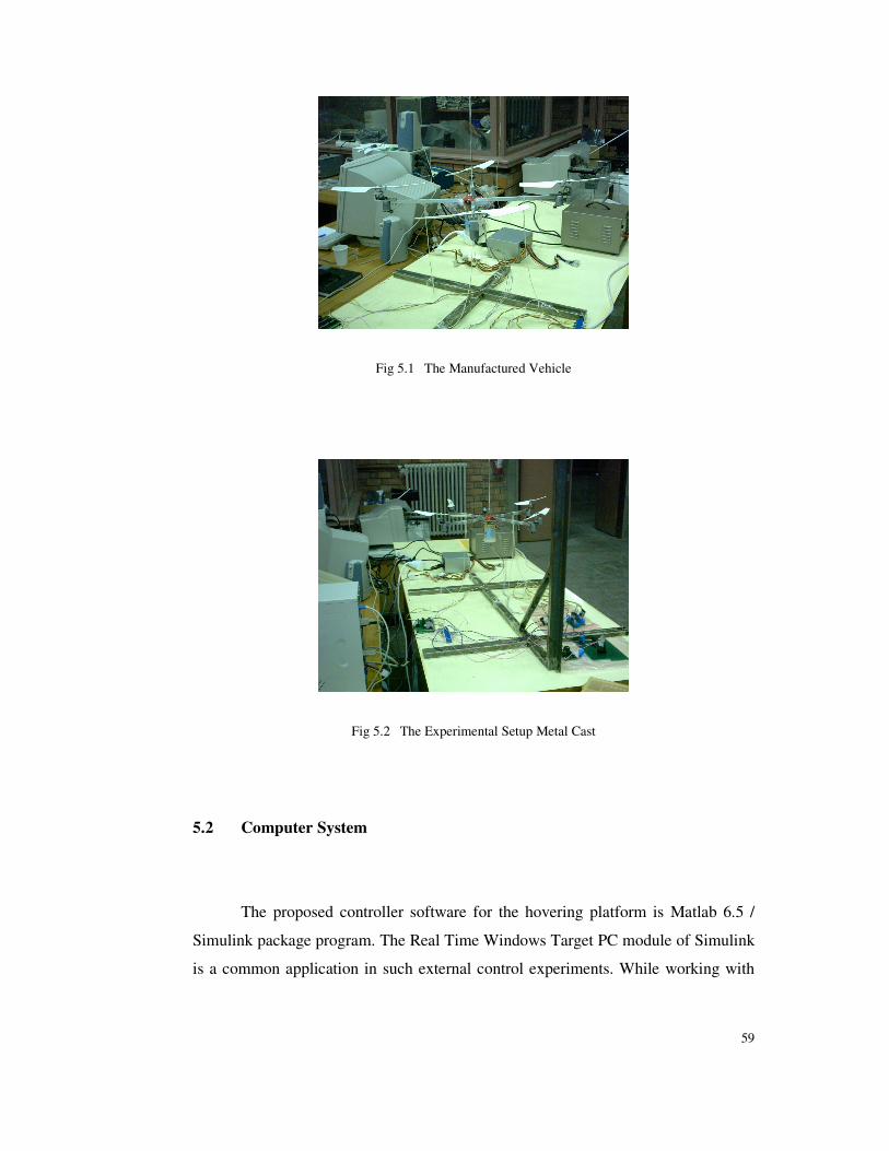
59

Fig 5.1 The Manufactured Vehicle

Fig 5.2 The Experimental Setup Metal Cast

5.2 Computer System

The proposed controller software for the hovering platform is Matlab 6.5 /

Simulink package program. The Real Time Windows Target PC module of Simulink

is a common application in such external control experiments. While working with

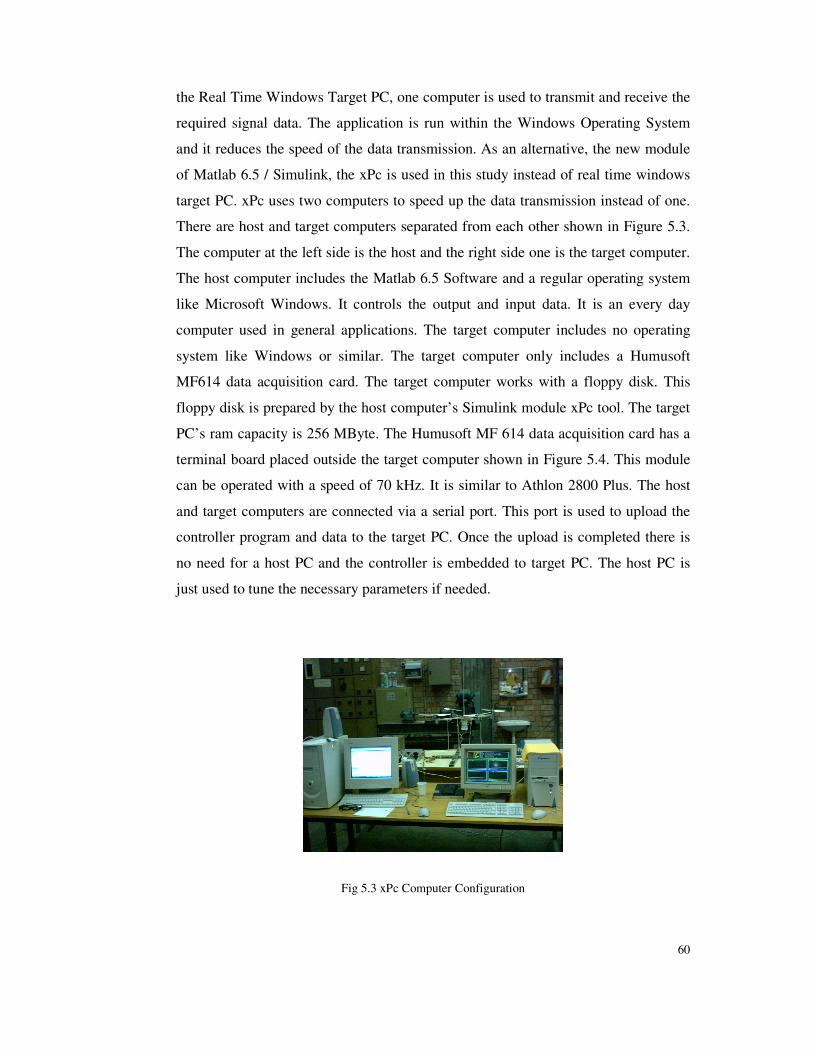
60

the Real Time Windows Target PC, one computer is used to transmit and receive the

required signal data. The application is run within the Windows Operating System

and it reduces the speed of the data transmission. As an alternative, the new module

of Matlab 6.5 / Simulink, the xPc is used in this study instead of real time windows

target PC. xPc uses two computers to speed up the data transmission instead of one.

There are host and target computers separated from each other shown in Figure 5.3.

The computer at the left side is the host and the right side one is the target computer.

The host computer includes the Matlab 6.5 Software and a regular operating system

like Microsoft Windows. It controls the output and input data. It is an every day

computer used in general applications. The target computer includes no operating

system like Windows or similar. The target computer only includes a Humusoft

MF614 data acquisition card. The target computer works with a floppy disk. This

floppy disk is prepared by the host computer’s Simulink module xPc tool. The target

PC’s ram capacity is 256 MByte. The Humusoft MF 614 data acquisition card has a

terminal board placed outside the target computer shown in Figure 5.4. This module

can be operated with a speed of 70 kHz. It is similar to Athlon 2800 Plus. The host

and target computers are connected via a serial port. This port is used to upload the

controller program and data to the target PC. Once the upload is completed there is

no need for a host PC and the controller is embedded to target PC. The host PC is

just used to tune the necessary parameters if needed.

Fig 5.3 xPc Computer Configuration

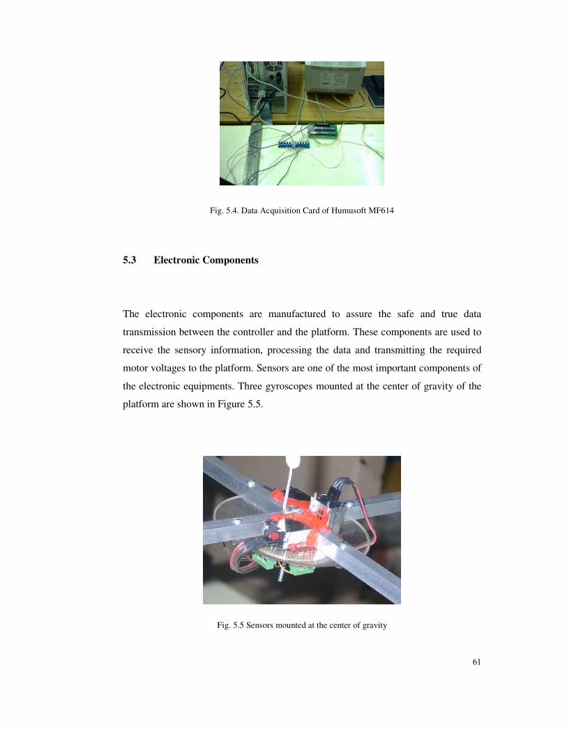
61

Fig. 5.4. Data Acquisition Card of Humusoft MF614

5.3 Electronic Components

The electronic components are manufactured to assure the safe and true data

transmission between the controller and the platform. These components are used to

receive the sensory information, processing the data and transmitting the required

motor voltages to the platform. Sensors are one of the most important components of

the electronic equipments. Three gyroscopes mounted at the center of gravity of the

platform are shown in Figure 5.5.

Fig. 5.5 Sensors mounted at the center of gravity

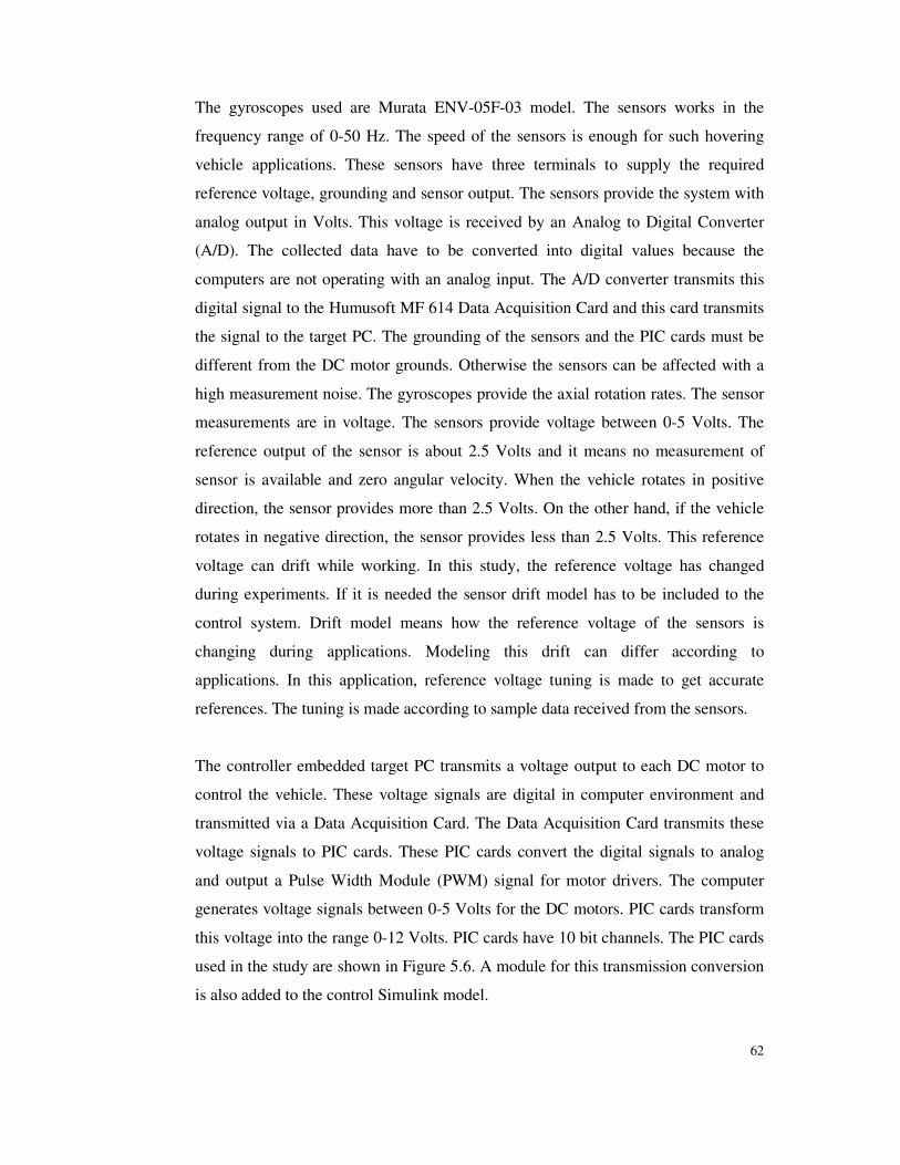
62

The gyroscopes used are Murata ENV-05F-03 model. The sensors works in the

frequency range of 0-50 Hz. The speed of the sensors is enough for such hovering

vehicle applications. These sensors have three terminals to supply the required

reference voltage, grounding and sensor output. The sensors provide the system with

analog output in Volts. This voltage is received by an Analog to Digital Converter

(A/D). The collected data have to be converted into digital values because the

computers are not operating with an analog input. The A/D converter transmits this

digital signal to the Humusoft MF 614 Data Acquisition Card and this card transmits

the signal to the target PC. The grounding of the sensors and the PIC cards must be

different from the DC motor grounds. Otherwise the sensors can be affected with a

high measurement noise. The gyroscopes provide the axial rotation rates. The sensor

measurements are in voltage. The sensors provide voltage between 0-5 Volts. The

reference output of the sensor is about 2.5 Volts and it means no measurement of

sensor is available and zero angular velocity. When the vehicle rotates in positive

direction, the sensor provides more than 2.5 Volts. On the other hand, if the vehicle

rotates in negative direction, the sensor provides less than 2.5 Volts. This reference

voltage can drift while working. In this study, the reference voltage has changed

during experiments. If it is needed the sensor drift model has to be included to the

control system. Drift model means how the reference voltage of the sensors is

changing during applications. Modeling this drift can differ according to

applications. In this application, reference voltage tuning is made to get accurate

references. The tuning is made according to sample data received from the sensors.

The controller embedded target PC transmits a voltage output to each DC motor to

control the vehicle. These voltage signals are digital in computer environment and

transmitted via a Data Acquisition Card. The Data Acquisition Card transmits these

voltage signals to PIC cards. These PIC cards convert the digital signals to analog

and output a Pulse Width Module (PWM) signal for motor drivers. The computer

generates voltage signals between 0-5 Volts for the DC motors. PIC cards transform

this voltage into the range 0-12 Volts. PIC cards have 10 bit channels. The PIC cards

used in the study are shown in Figure 5.6. A module for this transmission conversion

is also added to the control Simulink model.

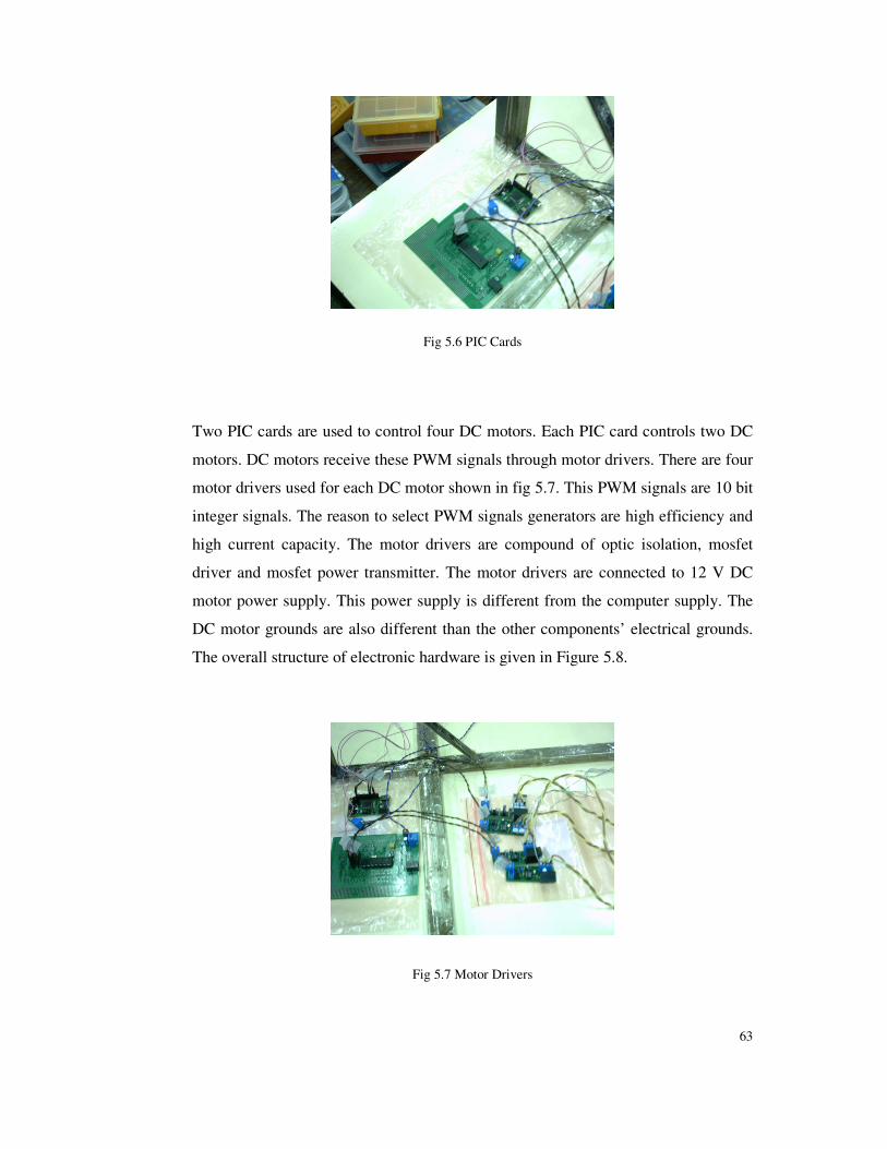
63

Fig 5.6 PIC Cards

Two PIC cards are used to control four DC motors. Each PIC card controls two DC

motors. DC motors receive these PWM signals through motor drivers. There are four

motor drivers used for each DC motor shown in fig 5.7. This PWM signals are 10 bit

integer signals. The reason to select PWM signals generators are high efficiency and

high current capacity. The motor drivers are compound of optic isolation, mosfet

driver and mosfet power transmitter. The motor drivers are connected to 12 V DC

motor power supply. This power supply is different from the computer supply. The

DC motor grounds are also different than the other components’ electrical grounds.

The overall structure of electronic hardware is given in Figure 5.8.

Fig 5.7 Motor Drivers

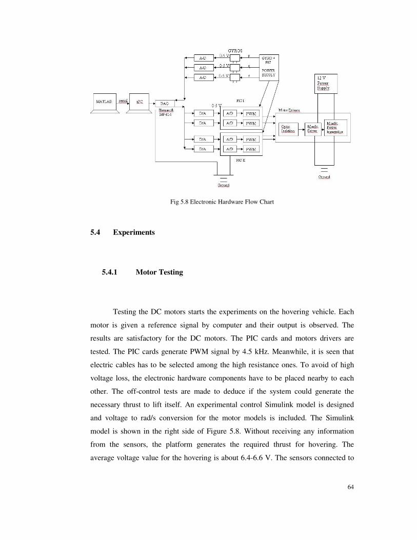
64

Fig 5.8 Electronic Hardware Flow Chart

5.4 Experiments

5.4.1 Motor Testing

Testing the DC motors starts the experiments on the hovering vehicle. Each

motor is given a reference signal by computer and their output is observed. The

results are satisfactory for the DC motors. The PIC cards and motors drivers are

tested. The PIC cards generate PWM signal by 4.5 kHz. Meanwhile, it is seen that

electric cables has to be selected among the high resistance ones. To avoid of high

voltage loss, the electronic hardware components have to be placed nearby to each

other. The off-control tests are made to deduce if the system could generate the

necessary thrust to lift itself. An experimental control Simulink model is designed

and voltage to rad/s conversion for the motor models is included. The Simulink

model is shown in the right side of Figure 5.8. Without receiving any information

from the sensors, the platform generates the required thrust for hovering. The

average voltage value for the hovering is about 6.4-6.6 V. The sensors connected to

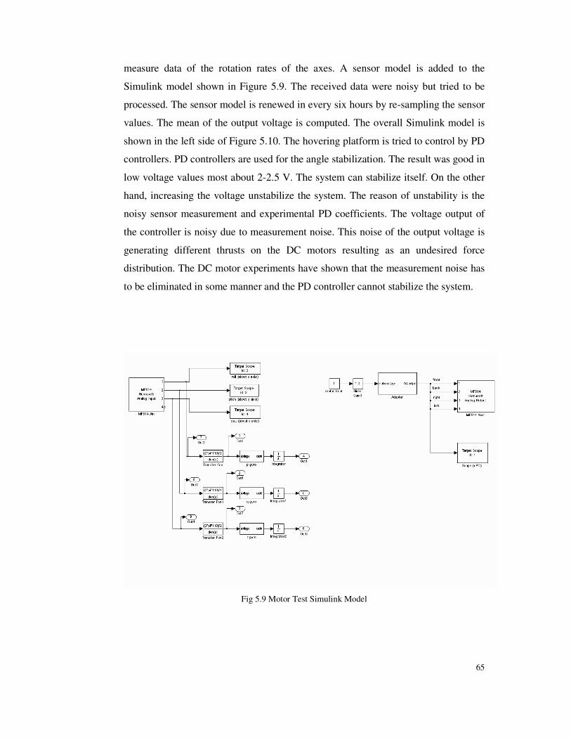
65

measure data of the rotation rates of the axes. A sensor model is added to the

Simulink model shown in Figure 5.9. The received data were noisy but tried to be

processed. The sensor model is renewed in every six hours by re-sampling the sensor

values. The mean of the output voltage is computed. The overall Simulink model is

shown in the left side of Figure 5.10. The hovering platform is tried to control by PD

controllers. PD controllers are used for the angle stabilization. The result was good in

low voltage values most about 2-2.5 V. The system can stabilize itself. On the other

hand, increasing the voltage unstabilize the system. The reason of unstability is the

noisy sensor measurement and experimental PD coefficients. The voltage output of

the controller is noisy due to measurement noise. This noise of the output voltage is

generating different thrusts on the DC motors resulting as an undesired force

distribution. The DC motor experiments have shown that the measurement noise has

to be eliminated in some manner and the PD controller cannot stabilize the system.

Fig 5.9 Motor Test Simulink Model

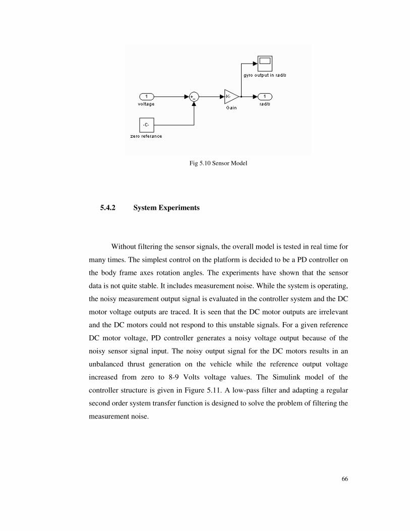
66

Fig 5.10 Sensor Model

5.4.2 System Experiments

Without filtering the sensor signals, the overall model is tested in real time for

many times. The simplest control on the platform is decided to be a PD controller on

the body frame axes rotation angles. The experiments have shown that the sensor

data is not quite stable. It includes measurement noise. While the system is operating,

the noisy measurement output signal is evaluated in the controller system and the DC

motor voltage outputs are traced. It is seen that the DC motor outputs are irrelevant

and the DC motors could not respond to this unstable signals. For a given reference

DC motor voltage, PD controller generates a noisy voltage output because of the

noisy sensor signal input. The noisy output signal for the DC motors results in an

unbalanced thrust generation on the vehicle while the reference output voltage

increased from zero to 8-9 Volts voltage values. The Simulink model of the

controller structure is given in Figure 5.11. A low-pass filter and adapting a regular

second order system transfer function is designed to solve the problem of filtering the

measurement noise.

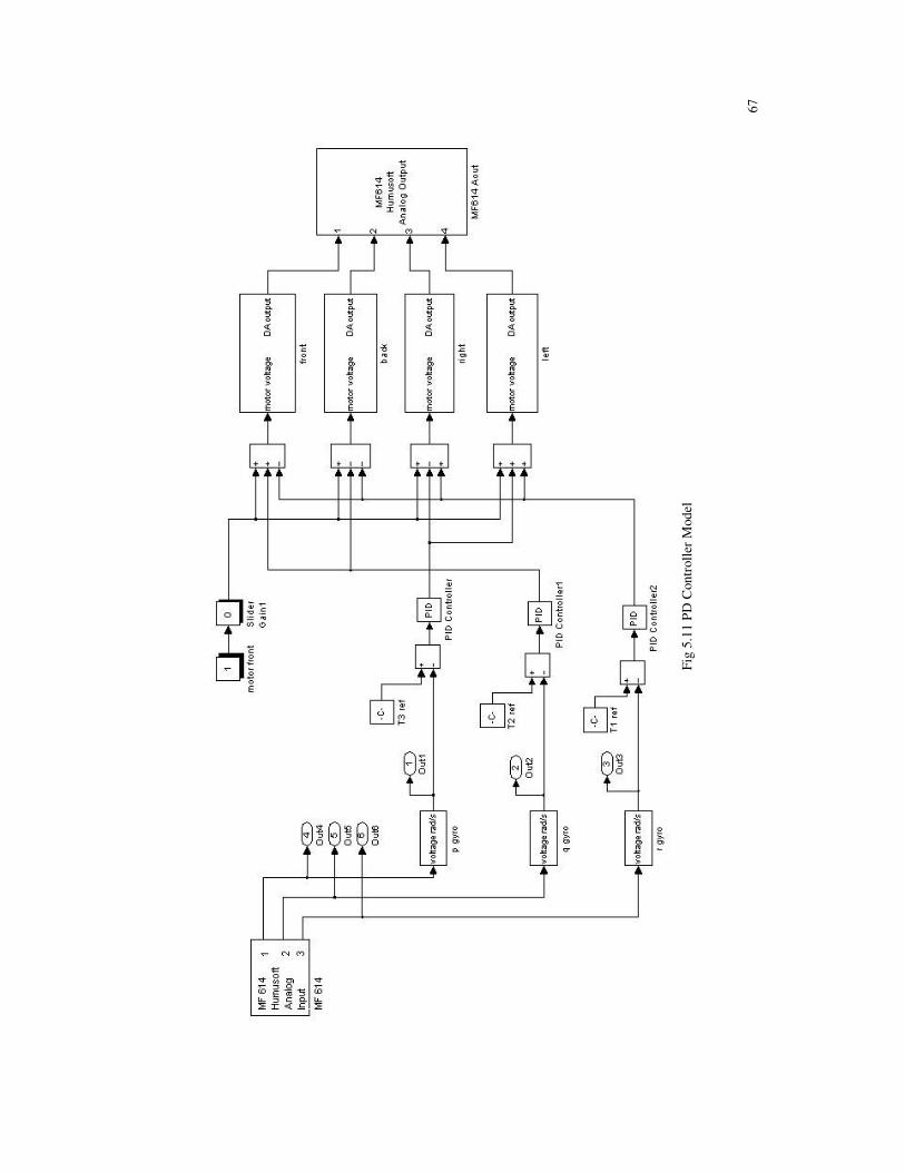
67

Fi

g 5.

11 P

D C

ontr

olle

r M

odel

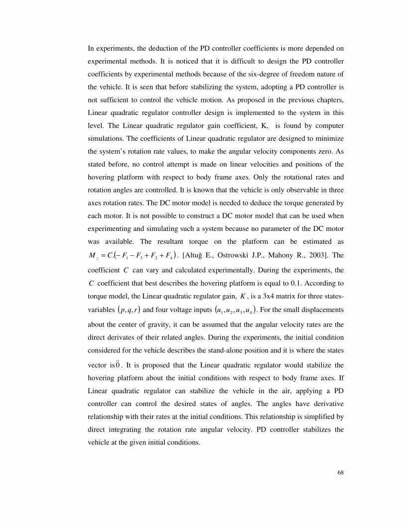
68

In experiments, the deduction of the PD controller coefficients is more depended on

experimental methods. It is noticed that it is difficult to design the PD controller

coefficients by experimental methods because of the six-degree of freedom nature of

the vehicle. It is seen that before stabilizing the system, adopting a PD controller is

not sufficient to control the vehicle motion. As proposed in the previous chapters,

Linear quadratic regulator controller design is implemented to the system in this

level. The Linear quadratic regulator gain coefficient, K, is found by computer

simulations. The coefficients of Linear quadratic regulator are designed to minimize

the system’s rotation rate values, to make the angular velocity components zero. As

stated before, no control attempt is made on linear velocities and positions of the

hovering platform with respect to body frame axes. Only the rotational rates and

rotation angles are controlled. It is known that the vehicle is only observable in three

axes rotation rates. The DC motor model is needed to deduce the torque generated by

each motor. It is not possible to construct a DC motor model that can be used when

experimenting and simulating such a system because no parameter of the DC motor

was available. The resultant torque on the platform can be estimated as

( )4231. FFFFCM z ++−−= . [Altu� E., Ostrowski J.P., Mahony R., 2003]. The

coefficient C can vary and calculated experimentally. During the experiments, the

C coefficient that best describes the hovering platform is equal to 0.1. According to

torque model, the Linear quadratic regulator gain, K , is a 3x4 matrix for three states-

variables ( )rqp ,, and four voltage inputs ( )4321 ,,, uuuu . For the small displacements

about the center of gravity, it can be assumed that the angular velocity rates are the

direct derivates of their related angles. During the experiments, the initial condition

considered for the vehicle describes the stand-alone position and it is where the states

vector is 0�

. It is proposed that the Linear quadratic regulator would stabilize the

hovering platform about the initial conditions with respect to body frame axes. If

Linear quadratic regulator can stabilize the vehicle in the air, applying a PD

controller can control the desired states of angles. The angles have derivative

relationship with their rates at the initial conditions. This relationship is simplified by

direct integrating the rotation rate angular velocity. PD controller stabilizes the

vehicle at the given initial conditions.

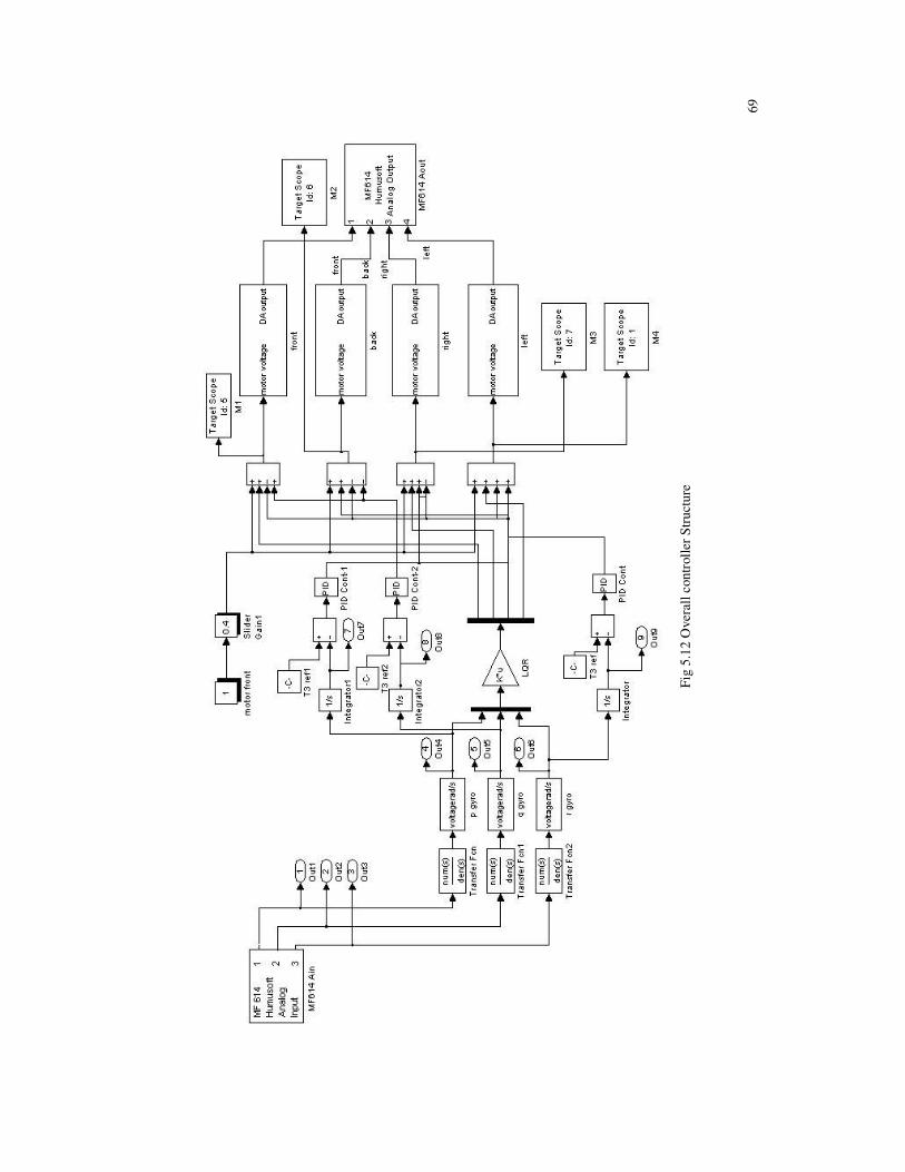
69

Fi

g 5.

12 O

vera

ll co

ntro

ller S

truc

ture

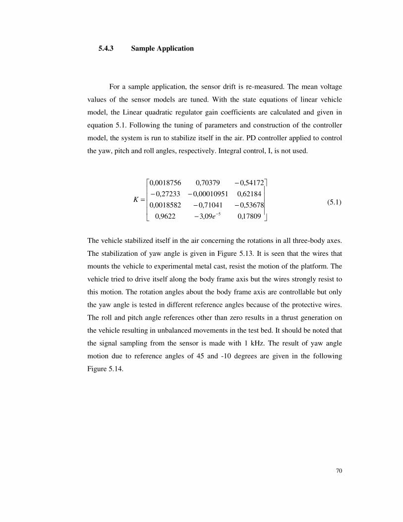
70

5.4.3 Sample Application

For a sample application, the sensor drift is re-measured. The mean voltage

values of the sensor models are tuned. With the state equations of linear vehicle

model, the Linear quadratic regulator gain coefficients are calculated and given in

equation 5.1. Following the tuning of parameters and construction of the controller

model, the system is run to stabilize itself in the air. PD controller applied to control

the yaw, pitch and roll angles, respectively. Integral control, I, is not used.

(5.1)

The vehicle stabilized itself in the air concerning the rotations in all three-body axes.

The stabilization of yaw angle is given in Figure 5.13. It is seen that the wires that

mounts the vehicle to experimental metal cast, resist the motion of the platform. The

vehicle tried to drive itself along the body frame axis but the wires strongly resist to

this motion. The rotation angles about the body frame axis are controllable but only

the yaw angle is tested in different reference angles because of the protective wires.

The roll and pitch angle references other than zero results in a thrust generation on

the vehicle resulting in unbalanced movements in the test bed. It should be noted that

the signal sampling from the sensor is made with 1 kHz. The result of yaw angle

motion due to reference angles of 45 and -10 degrees are given in the following

Figure 5.14.

��

��

�

−−−

−−−

=

− 17809,009,39622,053678,071041,00018582,0

62184,000010951,027233,054172,070379,00018756,0

5e

K

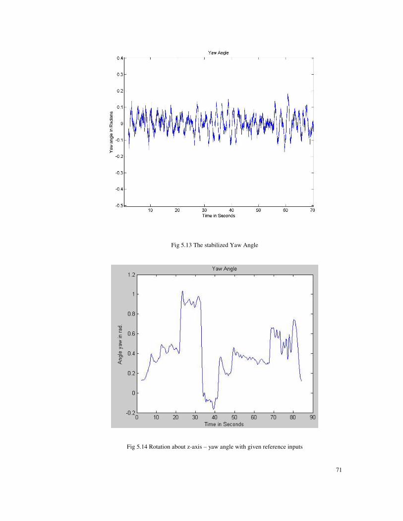
71

Fig 5.13 The stabilized Yaw Angle

Fig 5.14 Rotation about z-axis – yaw angle with given reference inputs

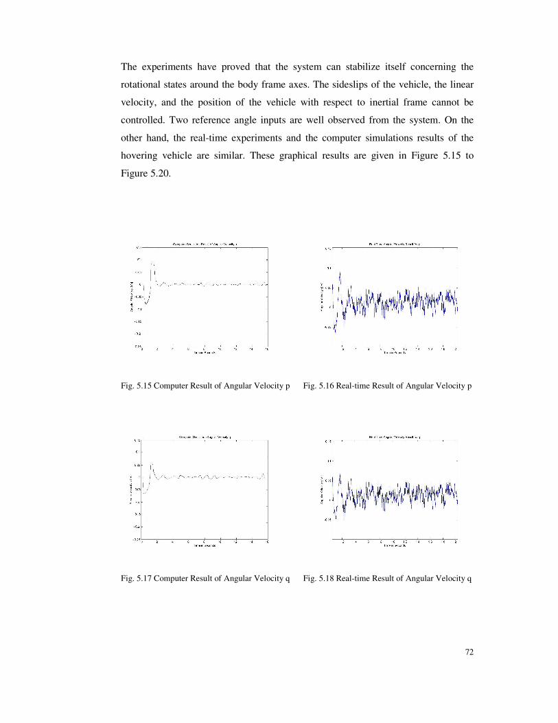
72

The experiments have proved that the system can stabilize itself concerning the

rotational states around the body frame axes. The sideslips of the vehicle, the linear

velocity, and the position of the vehicle with respect to inertial frame cannot be

controlled. Two reference angle inputs are well observed from the system. On the

other hand, the real-time experiments and the computer simulations results of the

hovering vehicle are similar. These graphical results are given in Figure 5.15 to

Figure 5.20.

Fig. 5.15 Computer Result of Angular Velocity p Fig. 5.16 Real-time Result of Angular Velocity p

Fig. 5.17 Computer Result of Angular Velocity q Fig. 5.18 Real-time Result of Angular Velocity q

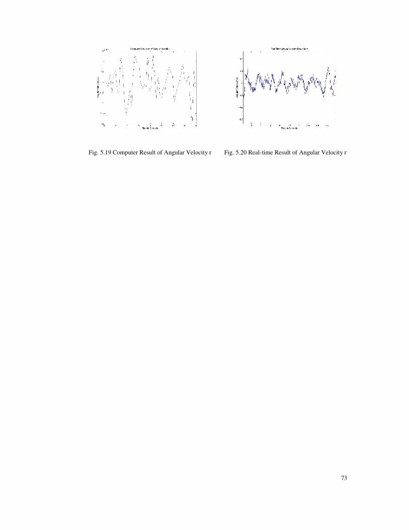
73

Fig. 5.19 Computer Result of Angular Velocity r Fig. 5.20 Real-time Result of Angular Velocity r

74

CHAPTER VI

CONCLUSIONS AND DISCUSSIONS

The system considered in this project is a four rotor hovering platform. The

manufacturing of the system is made using standard Aluminum structure and DC

motors. The propellers are commercially available hovering platform propellers. The

mass of the structure is 0.605 kg. The mass of the system is slightly heavy for such

an application. The possible mass reduction can be accomplished by using carbon

structure rather than Aluminum. This choice will result in 0.1-0.11 kg mass reduction

within the structure. Also, DC motor selection may be changed. The DC motors used

are not effective due to current drawn vs. thrust generation. The new choice of DC

motors can be mini brush-less motors. The DC motors used are 45 g each. The new

motor selections will result in approximately 30 g mass reduction. The

manufacturing of the structure directly affects the behavior of the system. In this

application, the manufacturing of the system was well suited and balanced.

Three gyroscopic sensors are used. These gyroscopes are not enough to control the

hovering vehicle, completely. With the given inertial measurement units, only the

rotational states can be controlled. The drift effect of the sensors is not modeled in

this study. For future studies, the drift effect can to be mathematically modeled.

Accelerometers are needed to sense the motion the linear velocity components along

the body axes. Increasing the number of sensors will result in more robust control.

The test bed used is sufficient in this application but can be renewed. The vehicle is

tied to the test bed. The wires cannot be mounted to the exact center of gravity. This

shifting resulted in undesired initial condition changes. Also, in simulation and

mathematical modeling, the effect of the wires can be re-considered. The upper and

75

lower wires can be omitted when linear velocities of the vehicle are controlled. The

electronic components are well designed for this application. During the

experiments, the electronic components had no problem. Only the A/D converters

have to be more sensitive. The tuning of the electronic components has to be well

suited to the structure manufactured. The PIC cards and motor drivers can be

dimensionally miniaturized for the future works and embedded on the vehicle. The

power source for the system is provided externally. The DC motors current drawn is

high. If the motors can be replaced with the mini brush-less ones and the mass can be

reduced, the system can be operated with onboard power sources.

The controller design for the system starts with the mathematical modeling. The

mathematical modeling and assumptions must be well suited to the manufactured

vehicle. The use of Matlab 6.5 / Simulink is efficient. Rather than using Real Time

Windows Target Pc module of Simulink, the use of xPc is a strong alternative tool.

Using PD controller is useless if the overall system is not stable. The PD controller

coefficients cannot be determined experimentally in six degree of freedom systems.

The coefficients needed to be selected after the overall structure stability is observed.

The Linear quadratic regulator design is a well choice for rotational stability. The

mathematical modeling and its linearized approximations are required to deduce the

feedback gain coefficients. Also, to use the Linear quadratic regulator more

effectively, the states of vehicle position and velocity have to be observed. The states

considered have to be observed using more sensors. The experiments have shown

that such a system with three gyroscopes cannot be fully controlled in the open air. It

is proposed that the future work can be focused on building lighter hovering

platforms and solving the obsevervability problems, the estimation problems, if it is

not possible to have information about all the system state-variables. The filtering

problem needed to be well design for real time applications.

76

REFERENCES

Altu� E., Mahony R., Ostrowski J. P., ”Control of a Quadrotor Helicopter Using Visual Feedback”, Robotics and Automation 2002 Proceedings, ICRA 02 IEEE International Conference, Volume 1, pages 72-77, May 2002,

Apkarian J., “Internet Control“, Circuit Cellar-The Magazine for Computer Applications, Issue 110, September 1999, Future Article, Retrieved October 2003, from http://www.circuitcellar.com/library/print/0999/Apkar110,

Borenstein, J. and Koren, Y., "Motion Control Analysis of a Mobile Robot" Transactions of ASME, Journal of Dynamics, Measurement and Control, Vol. 109, No. 2, pp. 73-79., October 1987,

Brogan W. L., “Modern Control Theory”, New Jersey, Prentice Hall, 1991,675-684,

Castillo P., Dzul A., Lozano R., “Real-time Stabilization and Tracking of a Four Rotor Mini-Rotorcraft”, IEEE Transactions on Control System Technology, Volume:12, Issue: 4 , Pages:510 – 516, July 2004,

Cheng M., Huzmezan M., "A Simulation Model and Hinf Loop shaping Control of a Quad Rotor Unmanned Air Vehicle”, Proceedings of MS’03 Conference, Palm Springs,CA, USA, February 2003, Retvied December 2003, from http://www.ece.ubc.ca/~huzmezan/pcopies.html,

D. Goshen-Meskin, “Observability Analysis of Piece-Wise Constant Systems-Part I: Theory”, IEEE Transactions in Aerospace and Electronic Systems, Vol. 28, No:4, October 1992, Dorf. R.C., Bishop R. H., “Modern Control Systems-Tenth Edition“, Prentice Hall, 2001, 110-123, Ellis R., Gulick D., “Calculus I and several variables”, Saunders, 1991, 714-716,

Gibb J., Jones C., Lee T., “A purpose Built Robot for Aerial Surveillance”. The University of British Columbia, 2001, Retrieved July 2002, from controls.ae.gatech.edu/gtar/ iarcpapers/british_columbia2000.pdf,

Hamel T., Mahony R., Lozano R., Ostrwski J., ”Dynamic Modeling and Configuration Stabilization for an X-4 Flyer ”, 15th Triennial World Congress-Spain, 2002, Retrieved August 2003, from http://www.hds.utc.fr/~helico/publications.html,

77

Hespanha J. P., “Optimal Control; LQR/LQG Controller Design“, Lecture Notes, May 1 2004, Retrieved May 2004, from http://www.ece.ucsb.edu/~hespanha/,

Judd K., “Nonlinear State Estimation, Indistinguishable States and Extended Kalman Filter”, Physica D 183, p:273-281, 2003.

Keennon M. T., Grasmayer J. M., “Development of Black Widow Micro Air Vehicle”. AeroVironment Inc., U.S., 2002, Retrieved January 2003, from www.aerovironment.com/ area-aircraft/prod-serv/bwidpap.pdf,

Kroo I., “Mesicopter Interim Reports”, Stanford University, 2001, Retrieved May 2002, from adg.stanford.edu/mesicopter/ProgressReports/,

Lewis F.L., “Control System Design Project Lecture Notes”, 1999, Retrieved February 2002, from http://arri.uta.edu/acs/ee4343/lectures99/rlocus2.pdf,

Marti S., ”The zero G eye: towards a free hovering camera” Technical report of final project, M.I.T. 2000, Retrieved June 2003, from http://web.media.mit.edu/- ~stefanm/HowTo/ZeroGEye.html, Michelson R.C., “Update on Flapping Wing Micro Air Vehicle Research”, Georgia Tech Research Institute, 2000, Retrieved May 2002, from http://avdil.gtri.- gatech.edu/RCM/RCM/Entomopter/EntomopterProject.html, Musial M., Hommel G., Brandenburg U. W., “Technische Universtat Berlin’s Flying Robot Competition at the IARC’99“, Technische Universitat Berlin, 1999, Retrieved May 2002, from http://pdv.cs.tu-berlin.de/leute/musial.html,

Nice E. B., “Design of a Four Rotor Hovering Vehicle”, Master Thesis in Cornell University, May 2004, Retrieved July 2004, from dspace.library.cornell.edu/ -bitstream/1813/93/2/Designof4RotHoverVehicle.pdf,

Oppenheim A.V., Schafer R. W., “Discrete-time Signal Processing“, Prentice Hall, 1999,

Yavrucuk, I.;Kannan, S.; Restrepo, C.; Wills, L.; Schrage, D.; Prasad, J.V.R.; “Control Algorithm and Flight Simulation Integration Using the Open Control Platform for Unmanned Aerial Vehicles” Digital Avionics Systems Conference, Proceedings. 18th, Volume: 2, 24-29 Pages:6.A.3-1 - 6.A.3-10 vol.2, Oct. 1999, Quanser Technical Report, 2002, Retrieved May 2003, from http://echo.ryerson.ca/flashcom/applications/controlsys/,

78

Saripalli S., Roberts J. M., Corke P. I., Buskey G., “A Tale Of Two Helicopters“, Proceedings of IEEE/RSJ International Conference on Intelligent Robots and Systems, pp: 805-810, October 2003,

Scala B. F. L., Bitmead R. R., James M. R., “Conditions for Stability of Extended Kalman Filter and their Application to the Frequency Tracking Problem”,�Signal Processing, IEEE Transactions on, Volume:44, Issue:3, Pages:739 – 742, March 1996, Taylor D., “The Hovering Platform” Department of Cybernetics, University of Reading,U.K., 2000, Retrieved September 2002, from http://logicalgenetics.com/hp/,

Technology Focus, “Murata Offers Advanced Electronic Components for robots”, Dempa Publications, Inc., 2002, Retrieved May 2004, from http://www.murata.com/articles/ta0255.pdf, Welch G., Bishop G. “An introduction to Kalman Filter”, University of North Carolina, 1997, Retrieved May 2002, from http://www.cs.unc.edu/~tracker/media/pdf/SIGGRAPH2001_CoursePack_08.pdf,

Zywno M. S., Pereira, D.; “Innovative Initiatives in Control Education at Ryerson Polytechnic University-Fuzzy-Logic Control of the 3D Helicopter Simulator”, American Control Conference, 2000. Proceedings of the 2000, Volume:6, Pages:3991 – 3995, 28-30, June 2000,

79

APPENDIX I

USER’S MANUAL

The user’s manual of the hovering vehicle can be split into two major categories.

First one is the hardware of the hovering vehicle. This part includes the electronic

equipments and their connections with each other including the hovering vehicle

itself. The second part is the software of the controller. Second part includes the

controller design on computer and Matlab Software communication of each device.

PART I:

THE ELECTRONIC EQUIPMENTS AND THEIR CONNECTIONS

The electronic and mechanical hardware used to operate the hovering vehicle are

as follows;

• 1 x Humusoft Data Acquisition Card

• 2 x PIC Card

• 4 x Motor Drivers

• 2 x Power Supply

• 1 x The Hovering Vehicle

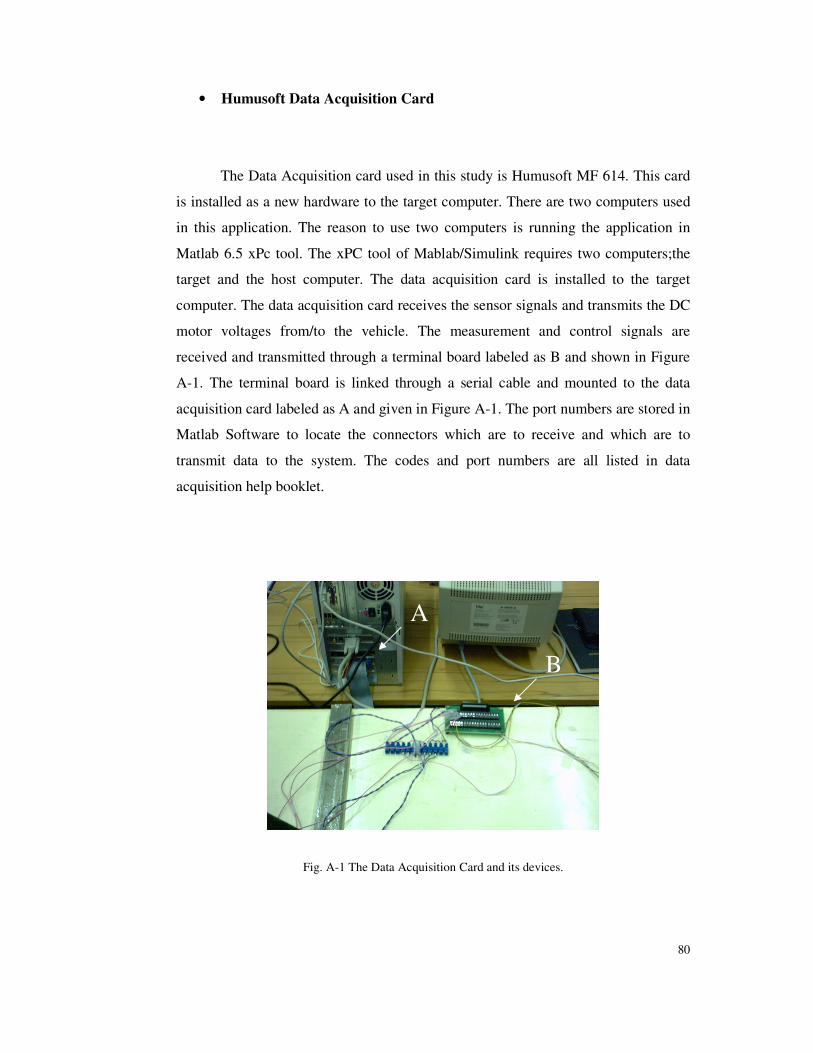
80

• Humusoft Data Acquisition Card

The Data Acquisition card used in this study is Humusoft MF 614. This card

is installed as a new hardware to the target computer. There are two computers used

in this application. The reason to use two computers is running the application in

Matlab 6.5 xPc tool. The xPC tool of Mablab/Simulink requires two computers;the

target and the host computer. The data acquisition card is installed to the target

computer. The data acquisition card receives the sensor signals and transmits the DC

motor voltages from/to the vehicle. The measurement and control signals are

received and transmitted through a terminal board labeled as B and shown in Figure

A-1. The terminal board is linked through a serial cable and mounted to the data

acquisition card labeled as A and given in Figure A-1. The port numbers are stored in

Matlab Software to locate the connectors which are to receive and which are to

transmit data to the system. The codes and port numbers are all listed in data

acquisition help booklet.

Fig. A-1 The Data Acquisition Card and its devices.

A

B

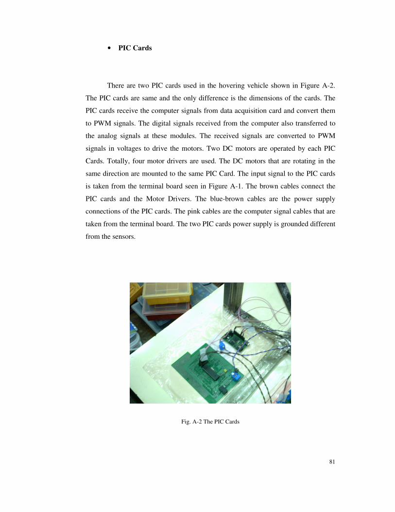
81

• PIC Cards

There are two PIC cards used in the hovering vehicle shown in Figure A-2.

The PIC cards are same and the only difference is the dimensions of the cards. The

PIC cards receive the computer signals from data acquisition card and convert them

to PWM signals. The digital signals received from the computer also transferred to

the analog signals at these modules. The received signals are converted to PWM

signals in voltages to drive the motors. Two DC motors are operated by each PIC

Cards. Totally, four motor drivers are used. The DC motors that are rotating in the

same direction are mounted to the same PIC Card. The input signal to the PIC cards

is taken from the terminal board seen in Figure A-1. The brown cables connect the

PIC cards and the Motor Drivers. The blue-brown cables are the power supply

connections of the PIC cards. The pink cables are the computer signal cables that are

taken from the terminal board. The two PIC cards power supply is grounded different

from the sensors.

Fig. A-2 The PIC Cards

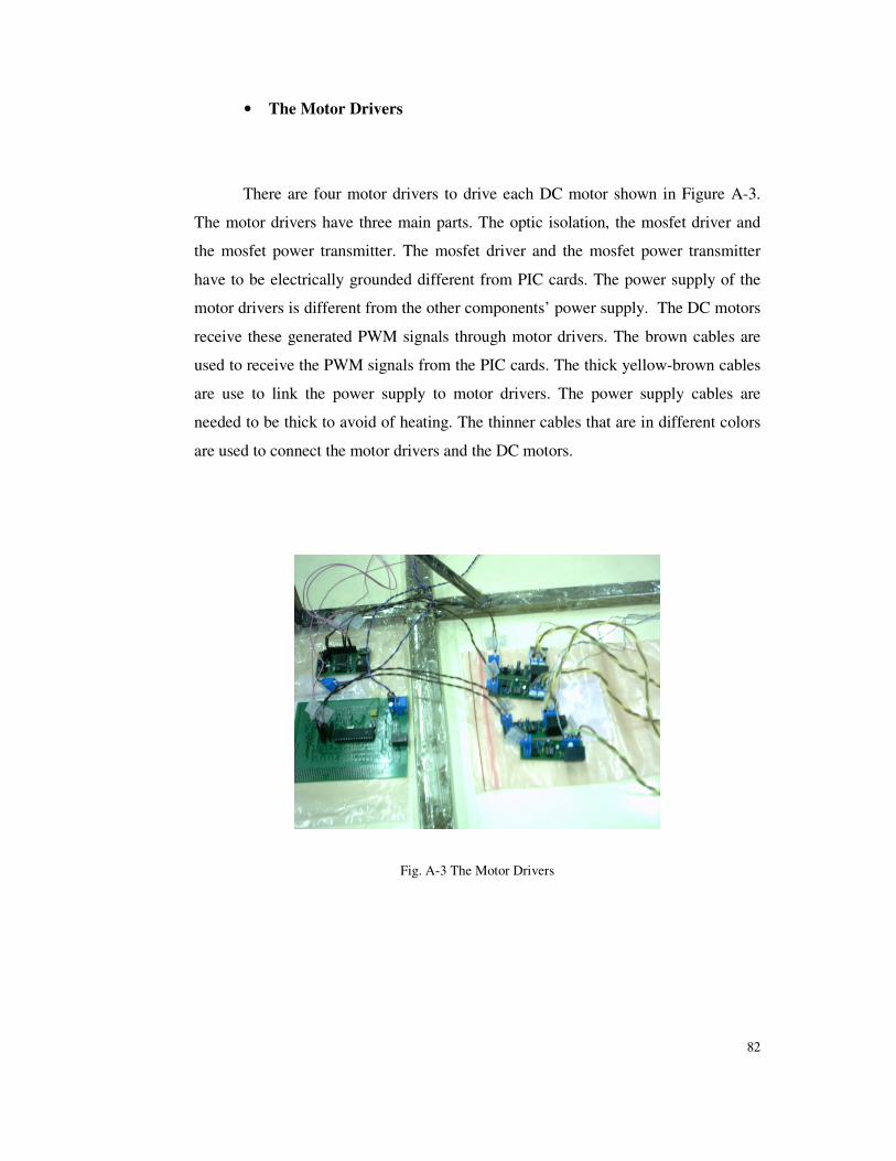
82

• The Motor Drivers

There are four motor drivers to drive each DC motor shown in Figure A-3.

The motor drivers have three main parts. The optic isolation, the mosfet driver and

the mosfet power transmitter. The mosfet driver and the mosfet power transmitter

have to be electrically grounded different from PIC cards. The power supply of the

motor drivers is different from the other components’ power supply. The DC motors

receive these generated PWM signals through motor drivers. The brown cables are

used to receive the PWM signals from the PIC cards. The thick yellow-brown cables

are use to link the power supply to motor drivers. The power supply cables are

needed to be thick to avoid of heating. The thinner cables that are in different colors

are used to connect the motor drivers and the DC motors.

Fig. A-3 The Motor Drivers

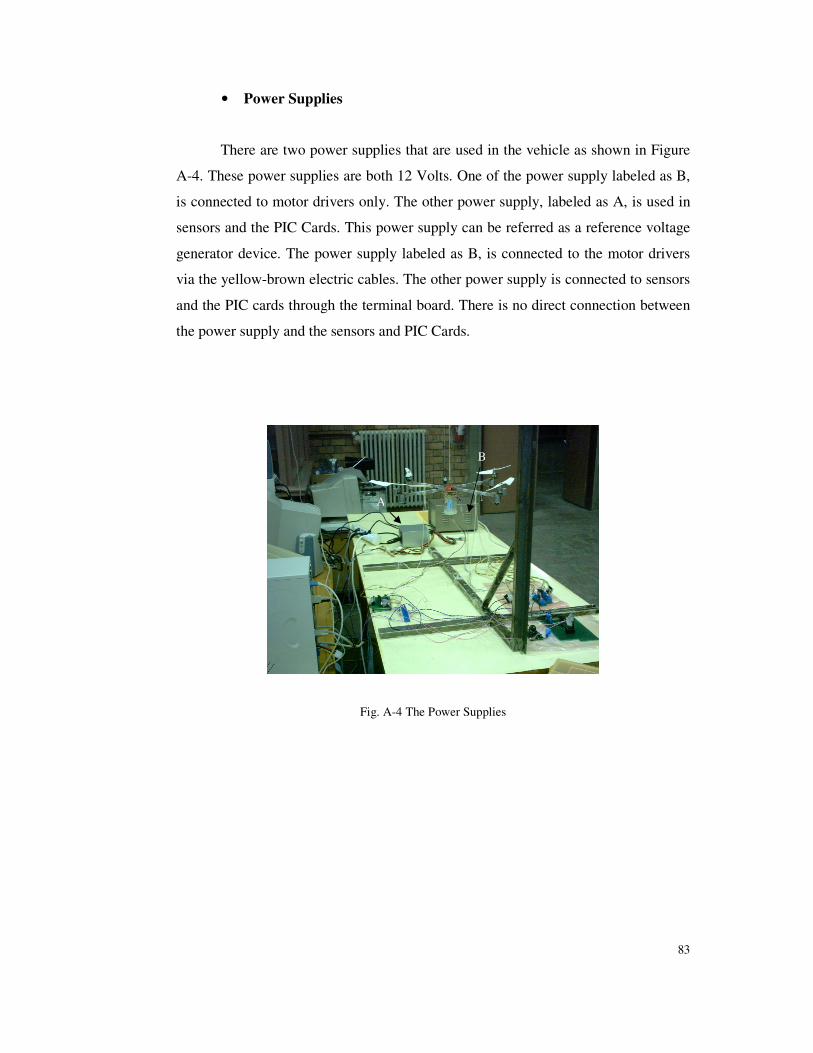
83

• Power Supplies

There are two power supplies that are used in the vehicle as shown in Figure

A-4. These power supplies are both 12 Volts. One of the power supply labeled as B,

is connected to motor drivers only. The other power supply, labeled as A, is used in

sensors and the PIC Cards. This power supply can be referred as a reference voltage

generator device. The power supply labeled as B, is connected to the motor drivers

via the yellow-brown electric cables. The other power supply is connected to sensors

and the PIC cards through the terminal board. There is no direct connection between

the power supply and the sensors and PIC Cards.

Fig. A-4 The Power Supplies

A

B

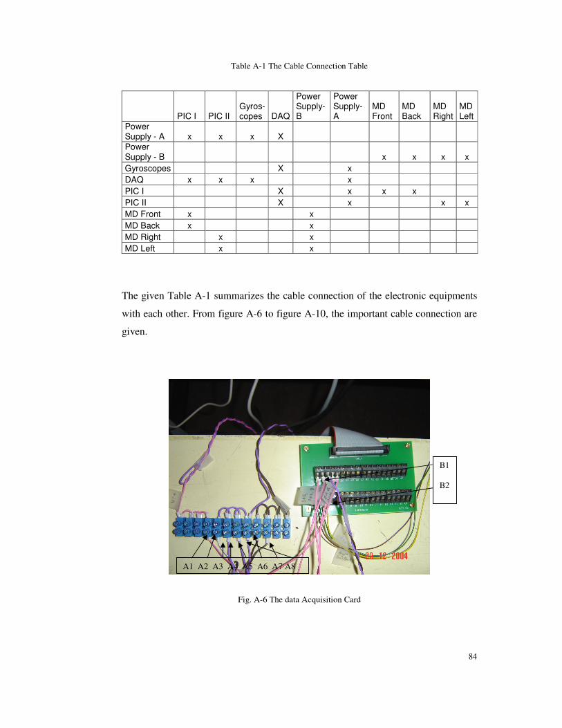
84

Table A-1 The Cable Connection Table

PIC I PIC II Gyros-copes DAQ

Power Supply-B

Power Supply-A

MD Front

MD Back

MD Right

MD Left

Power Supply - A x x x X Power Supply - B x x x x Gyroscopes X x DAQ x x x x PIC I X x x x PIC II X x x x MD Front x x MD Back x x MD Right x x MD Left x x

The given Table A-1 summarizes the cable connection of the electronic equipments

with each other. From figure A-6 to figure A-10, the important cable connection are

given.

Fig. A-6 The data Acquisition Card

A1 A2 A3 A4 A5 A6 A7 A8

B1 B2

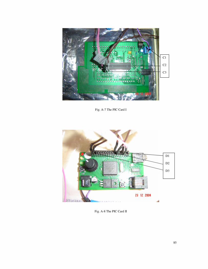
85

Fig. A-7 The PIC Card I

Fig. A-8 The PIC Card II

C1 C2 C3

D1 D2 D3

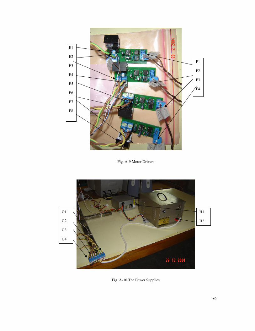
86

Fig. A-9 Motor Drivers

Fig. A-10 The Power Supplies

E1 E2 E3 E4 E5 E6 E7 E8

F1 F2 F3 F4

G1 G2 G3 G4

H1 H2

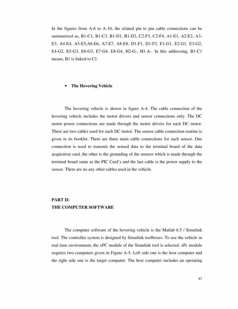
87

In the figures from A-6 to A-10, the related pin to pin cable connections can be

summarized as, B1-C1, B1-C3, B1-D1, B1-D2, C2-F3, C2-F4, A1-E1, A2-E2, A3-

E3, A4-E4, A5-E5,A6-E6, A7-E7, A8-E8, D1-F1, D1-F2, E1-G1, E2-G1, E3-G2,

E4-G2, E5-G3, E6-G3, E7-G4, E8-G4, H2-G-, H1-A-. In this addressing, B1-C1

means, B1 is linked to C1.

• The Hovering Vehicle

The hovering vehicle is shown in figure A-4. The cable connection of the

hovering vehicle includes the motor drivers and sensor connections only. The DC

motor power connections are made through the motor drivers for each DC motor.

There are two cables used for each DC motor. The sensor cable connection routine is

given in its booklet. There are three main cable connections for each sensor. One

connection is used to transmit the sensed data to the terminal board of the data

acquisition card, the other is the grounding of the sensors which is made through the

terminal board same as the PIC Card’s and the last cable is the power supply to the

sensor. There are no any other cables used in the vehicle.

PART II:

THE COMPUTER SOFTWARE

The computer software of the hovering vehicle is the Matlab 6.5 / Simulink

tool. The controller system is designed by Simulink toolboxes. To use the vehicle in

real time environment, the xPC module of the Simulink tool is selected. xPc module

requires two computers given in Figure A-5. Left side one is the host computer and

the right side one is the target computer. The host computer includes an operating

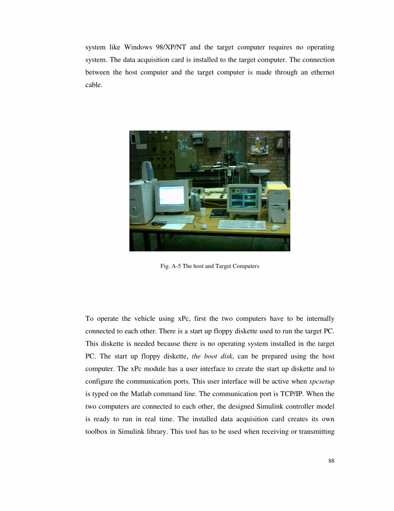
88

system like Windows 98/XP/NT and the target computer requires no operating

system. The data acquisition card is installed to the target computer. The connection

between the host computer and the target computer is made through an ethernet

cable.

Fig. A-5 The host and Target Computers

To operate the vehicle using xPc, first the two computers have to be internally

connected to each other. There is a start up floppy diskette used to run the target PC.

This diskette is needed because there is no operating system installed in the target

PC. The start up floppy diskette, the boot disk, can be prepared using the host

computer. The xPc module has a user interface to create the start up diskette and to

configure the communication ports. This user interface will be active when xpcsetup

is typed on the Matlab command line. The communication port is TCP/IP. When the

two computers are connected to each other, the designed Simulink controller model

is ready to run in real time. The installed data acquisition card creates its own

toolbox in Simulink library. This tool has to be used when receiving or transmitting

89

signal from or to vehicle. User can define many screens to follow the signals

received or transmitted in the target computer’s screen. Before starting the

application, some guidelines have to be outlined;

1- Make a new measurement of sensors drift values and re-new them in the controller

design. All the controller coefficients have to be checked. The building of the model

has to be made after this tuning is completed.

2- Built the controller model who ever wants to start a new controller test. The model

building operation can be made following tools � Real Time Workshop � Built

Model. If there is no error or warning prompt by Matlab, third step can be applied.

When the model is built, the target computer screen refreshes, too.

3- After the second step, the connect to target icon can be clicked on Simulink

window. At this step, it is advised that, someone should be ready to switch on/off the

power supplies due to an emergency.

4- Click on play icon.

5- Be sure that the voltage transmitted to the DC motors from controller is tuned to

zero or given a small value of 2 - 3 V. Switch on the power supply.

6- As the controller transmits voltage to the DC motors and receives the

measurement signal, the operation can be screened by target computer. During

operation, one can chance any reference value of voltage or angles.

7- To hover the vehicle, just increase the reference voltage values rapidly to 8-9 V.

8- To terminate the application, decrease the voltage value to zero and type stop in

the target computer command line and press disconnect from target icon in host

computer.

9- If the application is not stopped in the target computer, the data evaluation in the

host computer will not be possible.

10- In the host computer, type tg in the Matlab command screen. There are two

important points that have to be outlined in the tg menu. The time log and the output

log. The time log, stores the time and the output log stores the output results that are

defined before the application. An output can be defined using standard Simulink

output ports If the time and output logs are desired to be viewed, one should type

tg.OutputLog or tg.TimeLog in the command screen of Matlab.

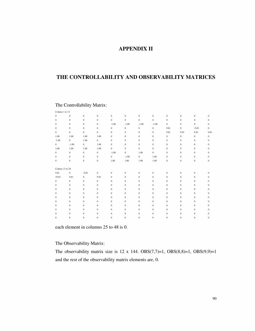
90

APPENDIX II

THE CONTROLLABILITY AND OBSERVABILITY MATRICES

The Controllability Matrix: Colums 1 to 12

0 0 0 0 0 0 0 0 0 0 0 0

0 0 0 0 0 0 0 0 0 0 0 0

0 0 0 0 -1.00 -1.00 -1.00 -1.00 0 0 0 0

0 0 0 0 0 0 0 0 9.81 0 -9.81 0

0 0 0 0 0 0 0 0 9.81 9.81 9.81 9.81

1.00 1.00 1.00 1.00 0 0 0 0 0 0 0 0

-1.00 0 1.00 0 0 0 0 0 0 0 0 0

0 -1.00 0 1.00 0 0 0 0 0 0 0 0

1.00 1.00 1.00 1.00 0 0 0 0 0 0 0 0

0 0 0 0 -1.00 0 1.00 0 0 0 0 0

0 0 0 0 0 -1.00 0 1.00 0 0 0 0

0 0 0 0 1.00 1.00 1.00 1.00 0 0 0 0

Colums 13 to 24

9.81 0 -9.81 0 0 0 0 0 0 0 0 0

19.62 9.81 0 9.81 0 0 0 0 0 0 0 0

0 0 0 0 0 0 0 0 0 0 0 0

0 0 0 0 0 0 0 0 0 0 0 0

0 0 0 0 0 0 0 0 0 0 0 0

0 0 0 0 0 0 0 0 0 0 0 0

0 0 0 0 0 0 0 0 0 0 0 0

0 0 0 0 0 0 0 0 0 0 0 0

0 0 0 0 0 0 0 0 0 0 0 0

0 0 0 0 0 0 0 0 0 0 0 0

0 0 0 0 0 0 0 0 0 0 0 0

0 0 0 0 0 0 0 0 0 0 0 0

each element in columns 25 to 48 is 0.

The Observability Matrix:

The observability matrix size is 12 x 144. OBS(7,7)=1, OBS(8,8)=1, OBS(9,9)=1

and the rest of the observability matrix elements are, 0.

DEMONSTRATION OF A STABILIZED HOVERING PLATFORM …etd.lib.metu.edu.tr/upload/12605772/index.pdf ·...

Documents

Transcript of DEMONSTRATION OF A STABILIZED HOVERING PLATFORM …etd.lib.metu.edu.tr/upload/12605772/index.pdf ·...