BEC 30325: MANAGERIAL ECONOMICS

DEMAND FORECASTING (PART – II)

Session 06

Dr. Sumudu Perera

• Smoothing Techniques-

• Example- Moving Average

• Limitations of Qualitative Demand

Forecasting

• Limitations of Quantitative Demand

Forecasting

Session Outline

Dr.Sumudu Perera 19/10/2017

2

Example- Moving Average

The following table shows the actual sales of

shoes of Boots Inc. from February 2016 to

August 2016

a) Compute 3 month moving average

forecasts

b) Compute 5 month moving average

forecasts

19/10/2017Dr.Sumudu Perera

3

Time (t) Month Sales (1000)

1 Feb 19

2 Mar 18

3 Apr 15

4 May 20

5 Jun 18

6 Jul 22

7 Aug 20

Limitations of Qualitative Forecasting

Techniques

Provides estimates that are dependent on the market skills of experts and their experience.

These skills differ from individual to individual.

Involves subjective judgment of the assessor, which may lead to over or under-estimation.

Depends on data provided by sales representatives who may have inadequate information

about the market.

Ignores factors, such as change in Gross National Product, availability of credit, and future

prospects of the industry, which may prove helpful in demand forecasting.

Most of the qualitative methods are expensive 19/10/2017Dr.Sumudu Perera

4

Limitations of Quantitative Forecasting

Techniques

There are many assumptions used in these statistical and mathematical models

Assumes that the past rate of changes in variables will remain same in future too,

which is not applicable in the practical situations.

Some techniques are quite complicated, managers may not be able to easily

understand

19/10/2017Dr.Sumudu Perera

5

BEC 30325: MANAGERIAL ECONOMICS

APPLICATION OF THEORY OF PRODUCTION

AND COST ANALYSIS (PART – I)

Session 07

Dr. Sumudu Perera

• Introduction

• The Production Function with one variable

input

• Optimal usage of the variable input

• The production with two variable inputs

• Optimal combination of two inputs

Session Outline

Dr.Sumudu Perera 19/10/2017

7

Theory of Production

Production - a process through which factor inputs are made into output that directly or indirectly satisfy consumer demand

PRODUCTION

SHORT RUN:

AT LEAST ONE

FIXED FACTOR &

GIVEN TECHNOLOGY

LONG RUN:

ALL FACTOR INPUTS

VARIABLE BUT NOT

technology

VERY LONG RUN:

ALL FACTOR INPUTS

AS WELL AS

TECHNOLOGY VARY

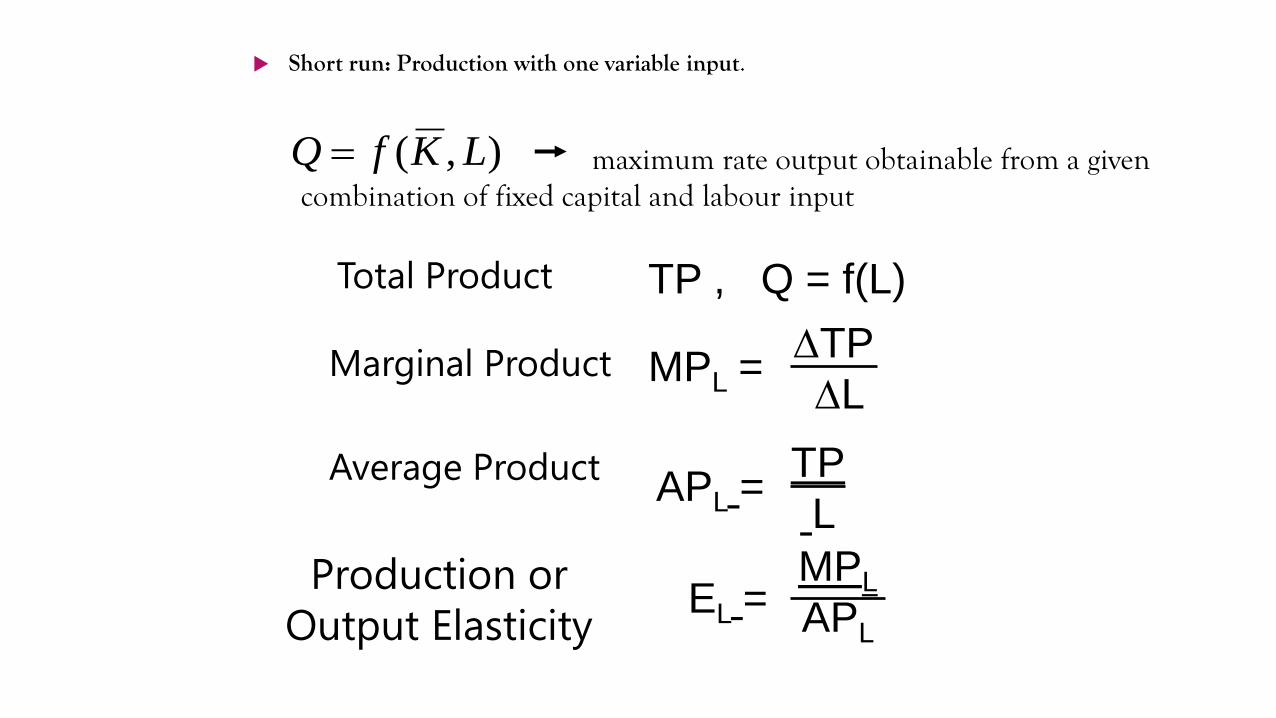
Short run: Production with one variable input.

maximum rate output obtainable from a given combination of fixed capital and labour input

),( LKfQ

Total Product

Marginal Product

Average Product

Production or

Output Elasticity

TP , Q = f(L)

MPL =TP

L

APL =TP

L

EL =MPL

APL

Output elasticity

It represents the change in the quantity produced as the change in with respect to the inputs

Eo = % change in output (ΔQ%)

% change in inputs (ΔX%)

or

= ΔQ x X

ΔX Q

Decision criteria: when Eo > 1 it reflects an increasing returns to scale, where Eo < 1 it reflects a

decreasing returns to scale and

Eo = 1 constant returns to scale.

Production Function with One

Variable Input

L Q MPL APL EL

0 0

1 3

2 8

3 12

4 14

5 14

Short Run Production Function

Short Run: Optimal Use of the Variable

Input

Marginal Revenue

Product of LaborMRPL = (MPL)(MR)

Marginal Resource

Cost of LaborMRCL =

TC

L

Optimal Use of Labor MRPL = MRCL

Optimal Use of the Variable Input

Optimal Use of the Variable Input

L MPL MR = P MRPL MRCL

2.50 4 $10 $40 $20

3.00 3 10 30 20

3.50 2 10 20 20

4.00 1 10 10 20

4.50 0 10 0 20

Use of Labor is Optimal When L = 3.50

Exercise : Optimal Variable Input Use

Labour Units Total Product Marginal

Product

Marginal

Revenue

Prodcut

Marginal

Resource Cost

0 0

1 5

2 15

3 45

4 55

5 60

6 68

7 55

Fill in the blanks.

Assume that the price of the product is Rs. 12 and wage cost is Rs. 360

Long run: Production with Two variable

inputs

Maximum rate output obtainable from a given combination of capital and labour input

which are variable

A firm faces with the problem of efficient allocation of resource in production, i.e., produce

output that maximizes profits.

Isoquants and Isocost

19/10/2017Dr.Sumudu Perera

17

),( LKfQ

Long Run: Production With Two Variable

Inputs

Firms will only use combinations of two

inputs that are in the economic region of

production, which is defined by the portion

of each iso-quant that is negatively sloped.

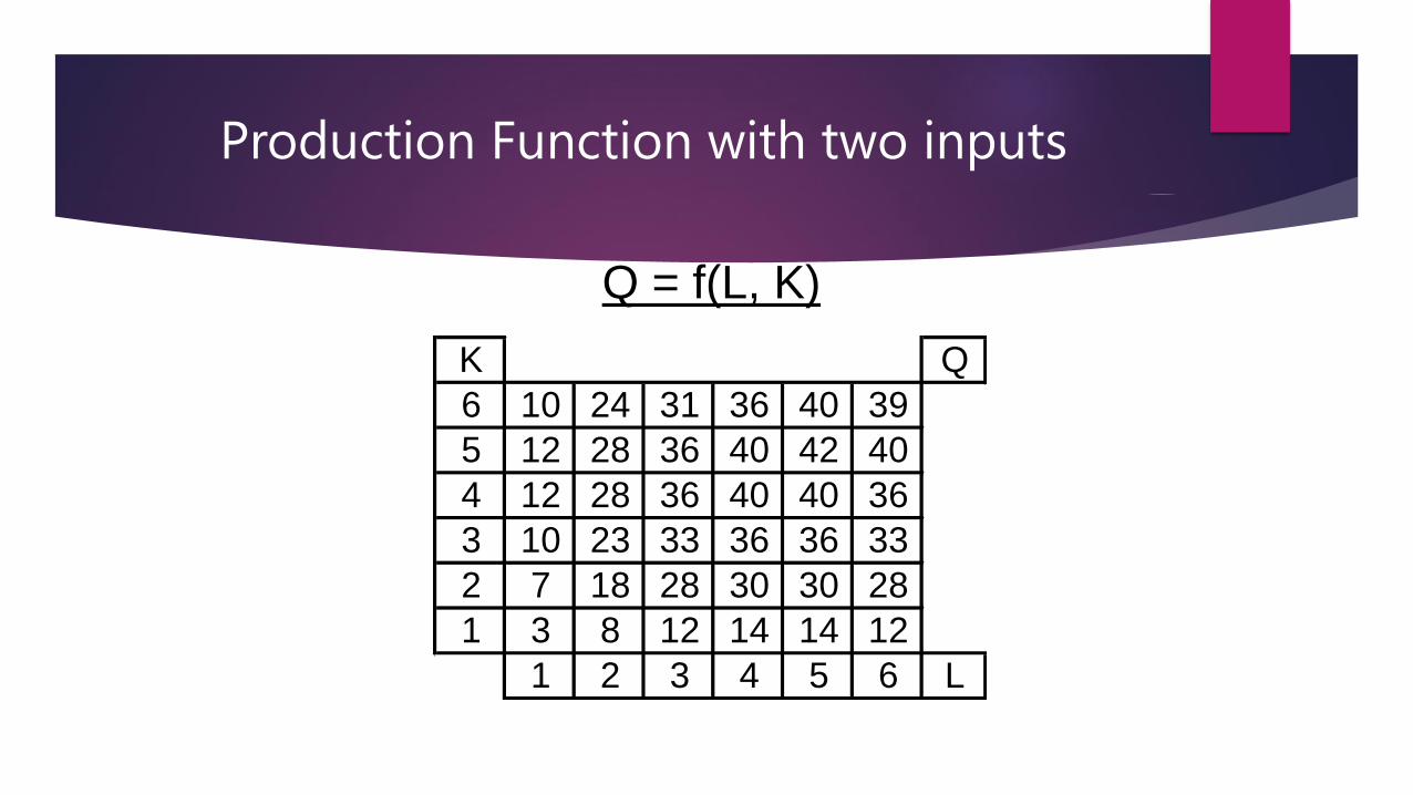
Production Function with two inputs

K Q

6 10 24 31 36 40 39

5 12 28 36 40 42 40

4 12 28 36 40 40 36

3 10 23 33 36 36 33

2 7 18 28 30 30 28

1 3 8 12 14 14 12

1 2 3 4 5 6 L

Q = f(L, K)

Production with two variable Inputs

Isoquants

Isocost

Ridge lines

MRTS and long run equilibrium

Production expansion path

Production with two variable inputs

Marginal Rate of Technical Substitution

MRTS = -K/L = MPL/MPK

Production With Two Variable Inputs

Substitute and Complementary inputs

Perfect

Substitutes

Perfect

Complements