Demand for Crash Insurance, Intermediary Constraints, and ... · on how the intermediaries manage...
68
Demand for Crash Insurance, Intermediary Constraints, and Risk Premia in Financial Markets Hui Chen Scott Joslin Sophie Ni * June 4, 2016 Abstract We propose a new measure of financial intermediary constraints based on how the intermediaries manage their tail risk exposures. Using a unique dataset for the trading activities in the market of deep out-of-the-money S&P 500 put options, we identify periods when the variations in the net amount of trading between financial intermediaries and public investors are likely to be mainly driven by shocks to intermediary constraints. We then infer tightness of intermediary constraints from the quantities of option trading during such periods. We show that a tightening of intermediary constraint according to our measure is associated with increasing option expensiveness, higher risk premia for a wide range of financial assets, deterioration in funding liquidity, and deleveraging of broker-dealers. * Chen: MIT Sloan and NBER ([email protected]). Joslin: USC Marshall ([email protected]). Ni: Hong Kong University of Science and Technology ([email protected]). We thank Tobias Adrian, David Bates, Robert Battalio, Geert Bekaert, Harjoat Bhamra, Ken French, Nicolae Garleanu, Zhiguo He, Bryan Kelly, Lei Lian, Andrew Lo, Dmitriy Muravyev, Jun Pan, Lasse Pedersen, Steve Ross, Ken Singleton, Moto Yogo, Hao Zhou, and seminar participants at USC, MIT Sloan, HKUST, Notre Dame, Washington University in St. Louis, New York Fed, Boston Fed, Copenhagen Business School, Dartmouth, AFA, the Consortium of Systemic Risk Analytics Meeting, CICF, SITE, the OptionMetrics Research Conference, and the Risk Management Conference at Mont Tremblant for comments, and Ernest Liu for excellent research assistance. We also thank Paul Stephens at CBOE, Gary Katz and Boris Ilyevsky at ISE for information on the option markets, and funding from Hong Kong RGC (644311).
Transcript of Demand for Crash Insurance, Intermediary Constraints, and ... · on how the intermediaries manage...

Demand for Crash Insurance, Intermediary Constraints,
and Risk Premia in Financial Markets
Hui Chen Scott Joslin Sophie Ni∗
June 4, 2016
Abstract
We propose a new measure of financial intermediary constraints based on how
the intermediaries manage their tail risk exposures. Using a unique dataset for the
trading activities in the market of deep out-of-the-money S&P 500 put options, we
identify periods when the variations in the net amount of trading between financial
intermediaries and public investors are likely to be mainly driven by shocks to
intermediary constraints. We then infer tightness of intermediary constraints from
the quantities of option trading during such periods. We show that a tightening of
intermediary constraint according to our measure is associated with increasing option
expensiveness, higher risk premia for a wide range of financial assets, deterioration
in funding liquidity, and deleveraging of broker-dealers.
∗Chen: MIT Sloan and NBER ([email protected]). Joslin: USC Marshall ([email protected]). Ni: HongKong University of Science and Technology ([email protected]). We thank Tobias Adrian, David Bates,Robert Battalio, Geert Bekaert, Harjoat Bhamra, Ken French, Nicolae Garleanu, Zhiguo He, BryanKelly, Lei Lian, Andrew Lo, Dmitriy Muravyev, Jun Pan, Lasse Pedersen, Steve Ross, Ken Singleton,Moto Yogo, Hao Zhou, and seminar participants at USC, MIT Sloan, HKUST, Notre Dame, WashingtonUniversity in St. Louis, New York Fed, Boston Fed, Copenhagen Business School, Dartmouth, AFA, theConsortium of Systemic Risk Analytics Meeting, CICF, SITE, the OptionMetrics Research Conference,and the Risk Management Conference at Mont Tremblant for comments, and Ernest Liu for excellentresearch assistance. We also thank Paul Stephens at CBOE, Gary Katz and Boris Ilyevsky at ISE forinformation on the option markets, and funding from Hong Kong RGC (644311).
1 Introduction
In this paper, we present new evidence connecting financial intermediary constraints to
asset prices. We propose to measure the tightness of intermediary constraints based
on how the intermediaries manage their aggregate tail risk exposures. Using a unique
dataset on the trading activities between public investors and financial intermediaries in
the market of deep out-of-the-money put options on the S&P 500 index (abbreviated as
DOTM SPX puts, which are insurance against market crashes), we identify periods when
shocks to intermediary constraints are likely to be the main driver of the variations in the
quantities of trading between public investors and financial intermediaries. This enables
us to infer tightness of intermediary constraints from the quantity of trading. We then
show that a tightening of intermediary constraint according to our measure is associated
with increasing option expensiveness, rising risk premia for a wide range of financial assets,
deterioration in funding liquidity, as well as deleveraging of broker-dealers.
To construct our measure, we start with the net amount of DOTM SPX puts that
public investors in aggregate acquire each month (henceforth referred to as PNBO), which
also reflects the net amount of the same options that broker-dealers and market-makers
sell in that month. While it is well known that financial intermediaries are net sellers of
these types of options during normal times, we find that PNBO varies significantly over
time and tends to turn negative during times of market distress.
Periods when PNBO is low could be periods of weak supply by intermediaries (due
to tight constraints) or weak demand by public investors. One needs to separate these
two effects before linking PNBO to intermediary constraints. We propose to exploit the
relation between the quantities of trading, measured by PNBO, and prices (expensiveness
of SPX options), as measured by the variance premium. Positive comovements in price and
quantity are consistent with the presence of demand shocks, while negative comovements
are consistent with the presence of supply shocks.1 We summarize the daily price-quantity
1We assume public investors’ demand curve is downward sloping, and financial intermediaries’ supplycurve is upward sloping. These assumptions apply when both groups are (effectively) risk averse andcannot fully unload the inventory risks through hedging. Notice that the presence of one type of shocksdoes not rule out the presence of the other.
1

relations into a monthly measure. Those months with negative price-quantity relations on
average are likely to be the periods when supply shocks are the main driver of the quantity
of trading. Then, we take low PNBO in a month with negative price-quantity relation as
indicative of tight intermediary constraints.
In monthly data from January 1991 to December 2012, PNBO is significantly negatively
related to the option expensiveness, and this negative relation becomes stronger when
jump risk in the market is higher. The correlation between PNBO and our measure of
option expensiveness in daily data is negative in 159 out of 264 months. These results
highlight the significant role that supply shocks play in the market of DOTM SPX puts.
During periods of negative price-quantity relation, PNBO significantly predicts future
market excess returns. A one-standard deviation decrease in PNBO (normalized PNBO)
in a month with negative price-quantity relation is on average associated with a 4.1% (3%)
increase in the subsequent 3-month log market excess return. The R2 of the regression
is 24.7% (12.3%). The predictive power of PNBO is even stronger in the months when
market jump risk is above the median level (in addition to the negative price-quantity
relation), but becomes much weaker in the months when the price-quantity relations are
positive. Besides equity, a lower PNBO also predicts higher future excess returns for
high-yield corporate bonds, an aggregate hedge fund portfolio, a carry trade portfolio, and
a commodity index, and it predicts lower future excess returns on long-term Treasuries
and (pay-fix) SPX variance swap.
The predictability results survive an extensive list of robustness checks. They include
different statistical methods for determining the significance of the predictive power,
exclusion of the 2008-09 financial crisis and extreme observations of PNBO, different ways
to define option moneyness, and an alternative quantity measure based on end-of-period
open interest instead of trading volume, etc. In addition, we consider an alternative
method for identifying periods of weak supply based on Rigobon (2003) (see also Sentana
and Fiorentini (2001)). Using the reduced-form econometric assumptions of this method,
we extract supply shocks and confirm the ability of the inferred supply shocks to predict
future stock returns.
2

The return predictability results are consistent with the intermediary asset pricing
theories, where a drop in the risk-sharing capacity of the financial intermediaries causes
the aggregate risk premium in the economy to rise. An alternative explanation of the
predictability results is that PNBO is merely a proxy for standard macro/financial factors
that simultaneously drive the aggregate risk premium and intermediary constraints. If
this alternative explanation is true, then the inclusion of proper risk factors into the
predictability regression should drive away the predictive power of our constraint measure.
We find that the predictive power of our measure is unaffected by the inclusion of a long list
of return predictors in the literature, including various price ratios, consumption-wealth
ratio, variance risk premium, default spread, term spread, and several tail risk measures.
While these results do not lead to the rejection of the alternative explanation (there can
always be omitted risk factors), they are at least consistent with intermediary constraints
having a unique effect on the aggregate risk premium.
Our intermediary constraint measure is significantly related to the funding liquidity
measure of Fontaine and Garcia (2012) and the measure of Adrian and Shin (2010) and
Adrian, Moench, and Shin (2010) based on the growth rate of broker-dealer leverage. We
also find that our constraint measure provides unique information about the aggregate
risk premium not contained in the other funding liquidity measures.
Our results suggest that when financial intermediaries switch from sellers of DOTM SPX
puts to buyers (e.g., in the months following the Lehman Brothers bankruptcy in 2008), it
is likely that the tightening of constraints are forcing the intermediaries to aggressively
hedge their tail risk exposures, rather than the intermediaries accommodating an increase
in public investors’ demand to sell crash insurance. Examples of shocks to intermediary
constraints include stricter regulatory requirements on banks’ tail risk exposures (e.g.,
due to the Dodd-Frank Act or Basel III), or losses incurred by the intermediaries. To
further understand the risk sharing mechanism, we try to identify who among the public
investors (retail or institutional) are the “liquidity providers” during times of distress:
reducing the net amount of crash insurance acquired from financial intermediaries or even
providing insurance to the latter group. We answer this question by comparing public
investors’ demand in the markets of SPX vs. SPY options. SPY options are options on the
3

SPDR S&P 500 ETF Trust, which has a significantly higher percentage of retail customers
than SPX options. Our results suggest that institutional public investors are the liquidity
providers during periods of distress.
Our paper builds on and extends the work of Garleanu, Pedersen, and Poteshman
(2009) (henceforth GPP) to incorporate supply shocks into the options market. In a
partial equilibrium setting, GPP demonstrate how exogenous public demand shocks affect
option prices when risk-averse dealers have to bear the inventory risks. In their model,
the dealers’ intermediation capacity is fixed, and the model implies a positive relation
between the public demand for options and the option premium. Like GPP, the limited
intermediation capacity of the dealers is a key assumption of ours, but we introduce shocks
to the intermediary risk-sharing capacity and then consider the endogenous relations
among public demand for options, option pricing, and aggregate market risk premium. In
the empirical analysis, we try to separate the effects of public demand shocks and shocks to
intermediary constraints, and show that the latter is linked to the time-varying risk premia
for a wide range of financial assets. Our empirical strategy based on the price-quantity
dynamics is motivated by Cohen, Diether, and Malloy (2007), who use a similar strategy
to identify demand and supply shocks in the equity shorting market.
The recent financial crisis has highlighted the importance of understanding the potential
impact of intermediary constraints on the financial markets and the real economy. Following
the seminal contributions by Bernanke and Gertler (1989), Kiyotaki and Moore (1997), and
Bernanke, Gertler, and Gilchrist (1999), recent theoretical developments include Gromb
and Vayanos (2002), Brunnermeier and Pedersen (2009), Geanakoplos (2009), He and
Krishnamurhty (2012), Adrian and Boyarchenko (2012), Brunnermeier and Sannikov (2013),
among others. We provide a reduced-form approach to model intermediary constraint,
which helps us derive quantitative predictions on the effects of time-varying intermediary
constraints in a tractable way.
In contrast to the fast growing body of theoretical work, there is relatively little
empirical work on measuring intermediary constraints and studying their aggregate effects
on asset prices. The notable exceptions include Adrian, Moench, and Shin (2010) and
4

Adrian, Etula, and Muir (2012), who show that changes in aggregate broker-dealer leverage
is linked to the time series and cross section of asset returns. Our paper demonstrates a
new venue (the crash insurance market) to capture intermediary constraint variations and
study their effects on asset prices. Moreover, compared to intermediary leverage changes,
our measure has the advantage of being forward-looking and available at higher (daily and
monthly instead of quarterly) frequency.
The ability of option volume to predict returns has been examined in other contexts.
Pan and Poteshman (2006) show that option volume predicts near future individual stock
returns (up to 2 weeks). They find the source of this predictability to be the nonpublic
information possessed by option traders. Our evidence of return predictability applies to
the market index and to longer horizons (up to 4 months), and we argue that the source
of this predictability is time-varying intermediary constraints.
Finally, several studies have examined the role that derivatives markets play in the
aggregate economy. Buraschi and Jiltsov (2006) study option pricing and trading volume
when investors have incomplete and heterogeneous information. Bates (2008) shows how
options can be used to complete the markets in the presence of crash risk. Longstaff and
Wang (2012) show that the credit market plays an important role in facilitating risk sharing
among heterogeneous investors. Chen, Joslin, and Tran (2012) show that the market risk
premium is highly sensitive to the amount of sharing of tail risks in equilibrium.
2 Research Design
Our goal is to measure how constrained financial intermediaries are through the ways they
manage the exposures to aggregate tail risks. The market of DOTM SPX put options
are well-suited for this purpose. First, this market is large in terms of the economic
exposures it provides for aggregate tail risks.2 Second, compared to other over-the-counter
derivatives that also provide exposures to aggregate tail risks, the exchange-traded SPX
2For example, based on data in December 2012, Johnson, Liang, and Liu (2014) estimate that thechange in total index option value is on the order of trillions of dollars following a severe market crash,the majority of which contributed by out-of-money SPX puts.
5
options have the advantages of better liquidity and removing counterparty risk (other than
exchange failure). Third, the Options Clearing Corporation (OCC) classifies exchange
option transactions by investor types, which is essential for measuring the net exposures
of the financial intermediaries.
Specifically, the OCC classifies each option transaction into one of three categories
based on who initiates the trade. They include public investors, firm investors, and
market-makers. Transactions initiated by public investors include those initiated by retail
investors and those by institutional investors such as hedge funds. Trades initiated by firm
investors are those that securities broker-dealers (who are not designated market-makers)
make for their own accounts or for another broker-dealer. Since we focus on financial
intermediaries as a whole, it is natural to merge firm investors and market-makers as one
group and observe how they trade against public investors.
We classify DOTM puts as those with strike-to-price ratio K/S ≤ 0.85. For robustness,
we also consider different strike-to-price cutoffs, as well as cutoffs that adjust for option
maturity and the volatility of the S&P 500 index (which is similar to cutoffs based on
option delta). Another feature of option transaction is that an order can either be an
open order (to open new positions) or a close order (to close existing positions). We will
focus on open orders, because they are less likely to be mechanically influenced by existing
positions (see Pan and Poteshman, 2006).
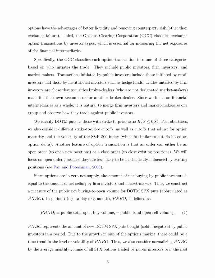
Since options are in zero net supply, the amount of net buying by public investors is
equal to the amount of net selling by firm investors and market-makers. Thus, we construct
a measure of the public net buying-to-open volume for DOTM SPX puts (abbreviated as
PNBO). In period t (e.g., a day or a month), PNBOt is defined as
PBNOt ≡ public total open-buy volumet − public total open-sell volumet. (1)
PNBO represents the amount of new DOTM SPX puts bought (sold if negative) by public
investors in a period. Due to the growth in size of the options market, there could be a
time trend in the level or volatility of PNBO. Thus, we also consider normalizing PNBO
by the average monthly volume of all SPX options traded by public investors over the past
6

three months,3
PNBONt ≡PNBOt
Average monthly public SPX volume over past 3 months. (2)
While PNBON helps address the potential issue with growth in the size of market,
PNBO has the advantage in that it better captures the actual magnitude of the tail risk
exposures being transferred between public investors and intermediaries, which matters for
measuring the degree of intermediary constraints. Considering this tradeoff, we conduct
all of our main analyses using both PNBO and PNBON .
It is well documented (see e.g., Bollen and Whaley, 2004) that public investors are net
buyers of index puts while financial intermediaries are net sellers during normal times.
All else equal, when financial intermediaries become more constrained, their willingness
to supply crash insurance to the market will be reduced. It is thus tempting to infer
how constrained financial intermediaries are based on the net amount of crash insurance
they sell to public investors each period, as captured by PNBO. However, besides weak
supply from constrained intermediaries, weak public demand can also cause the equilibrium
amount of crash insurance traded between public investors and intermediaries to be low.
The challenge is to separate the effects of supply from demand.
We address this problem by exploiting the price-quantity relation to identify periods of
“supply environments,” when variations in PNBO are likely to be mainly driven by shocks
to intermediary constraints.
Our quantity measure is PNBO. To measure the “price”, i.e., the expensiveness of
SPX options, one would ideally like to calculate the difference between the market price
of an option and its hypothetical price without any market frictions. The latter is not
observable and can only be approximated by adopting a specific structural model. For
simplicity and robustness, we use the variance premium (V P ) in Bekaert and Hoerova
(2014) as a proxy for overall expensiveness of SPX options, which is the difference between
VIX2 and the expected physical variance of the return of the S&P 500 index.4
3For robustness check, we also define PNBON using past 12-month average public trading volume inthe denominator, which generates similar results.
4The expected physical variance one month ahead (22 trading days) is computed using Model 8 in
7

Our empirical strategy is motivated by Cohen, Diether, and Malloy (2007) (CDM),
who identify shifts in demand vs. supply in the securities shorting market by examining the
relation between the changes in the loan fee (price) and the changes in the percentage of
outstanding shares on loan (quantity). In their setting, a simultaneous increase (decrease)
in the price and quantity indicates at least an increase (decrease) in shorting demand,
whereas an increase (decrease) in price coupled with a decrease (increase) in quantity
indicates at least a decrease (increase) in shorting supply.
The same logic applies to the options market. The demand pressure theory of GPP
predicts that a positive and exogenous shock to the public demand for DOTM SPX puts
forces risk-averse dealers to bear more inventory risks. As a result, the dealers will raise
the price of the option (a move along the upward-sloping supply curve). Thus, demand
shocks generate a positive relation between changes in prices and quantities. Alternatively,
if there are intermediation shocks that raise the degree of constraints facing financial
intermediaries (e.g., due to loss of capital or tightened capital requirements), they will
become less willing to provide crash insurance to public investors. Then, the premium for
the DOTM SPX puts rises while the equilibrium quantity of such options traded falls (a
move along the downward-sloping demand curve).
Different from CDM, we would like to identify periods of weak and strong supply
(level), instead of negative or positive supply shocks (changes). For this reason, we cannot
directly apply their identification strategy. However, the ability to identify supply and
demand shocks is still useful for our setting. Consider a month with low PNBO. If the
price-quantity relation suggests mainly supply shocks in that month, then the low PNBO
is more likely to be driven by weak supply instead of weak demand.
Based on this idea, we run the following regression using daily data in each month t:
V Pi(t) = aV P,t + bV P,t PNBOi(t) + dV P,t Ji(t) + εvi(t), (3)
Bekaert and Hoerova (2014): Ed
[RV
(22)d+1
]= 3.730 + 0.108
V IX2d
12 + 0.199RV(−22)d + 0.33 22
5 RV(−5)d + 0.107 ·
22RV(−1)d , where RV
(−j)d is the sum of daily realized variances from day d− j + 1 to day d. The daily
realized variance sums squared 5-minute intraday S&P500 returns and the squared close-to-open return.
8

where i(t) denotes day i in month t. The presence of jumps in the underlying stock index
can affect V P even when markets are frictionless. Thus, when examining the relation
between V P and PBNO, we control for the level of jump risk J in the S&P 500 index
based on the measure of Andersen, Bollerslev, and Diebold (2007).
A negative coefficient bV P,t < 0 in month t suggests that supply shocks are the dominant
driver of price-quantity relations in that month, and we expect PNBO to be informative
about the variation in intermediary constraints during such times. A negative coefficient
bV P,t < 0 does not identify any particular supply shock, nor does it rule out the presence
of demand shocks in the same month. It does indicate that supply shocks are likely to
be more significant relative to demand shocks. Similarly, bV P,t > 0 does not rule out the
presence of supply shocks in a month, but demand shocks are likely to be more significant.
During such periods, we do not expect PNBO to be informative about supply conditions.
Furthermore, we expect high jump risk to amplify the effect of shocks to intermediary
constraints on the equilibrium quantity of options traded. This is because a main reason
that intermediary constraint matters for their supply of DOTM index puts is the difficulty
to hedge the market jump risk embedded in their inventory positions. As long as public
demand does not become more volatile during such times (in fact, it seems reasonable
to assume that public demand will remain strong), variations in PNBO will be more
informative about shocks to intermediary constraints when jump risk is high. Thus, the
level of jump risk can further aid our identification of supply environments.
In summary, in a month when the price-quantity relation is on average negative
(bV P,t < 0), we expect small (or negative) value for PNBOt (cumulative net-buying by
public investors for the month) to indicate tight intermediary constraints.
Intermediary constraints and risk premia According to the theory of financial
intermediary constraints (see e.g., Gromb and Vayanos (2002) and He and Krishnamurhty
(2012)), variations in the aggregate intermediary constraints not only affect option prices,
but also drive the risk premia of other financial assets. This theory implies that low
PNBOt, when occurring in a period dominated by supply shocks, should imply high
future expected excess returns on the market portfolio. That is, we expect b−r < 0 in the
9

following predictive regression:
rt+j→t+k = ar + b−r I{bV P,t<0} PNBOt + b+r I{bV P,t≥0} PNBOt + cr I{bV P,t<0} + εt+j→t+k (4)
where r denotes log market excess return, and the notation t+ j → t+ k indicates the
leading period from t + j to t + k (k > j ≥ 0). Besides the market portfolio, the
predictability should apply to other risky assets as well.
The empirical strategy and testable hypotheses above are mainly based on economic
intuition. In Appendix A, we present a dynamic general equilibrium model featuring
time-varying intermediary constraints. The model not only helps formalize the main
intuition, but generates more rigorous predictions about how intermediary constraints
affect the equilibrium price-quantity dynamics in the crash insurance market, the aggregate
risk premium, and intermediary leverage. Moreover, we can use the calibrated model to
examine the quantitative effects of intermediary constraints on asset prices.
3 Empirical Results
We now present the empirical evidence connecting the option trading activities to the
constraints of the financial intermediaries, the pricing of index options, and the risk premia
in financial markets.
3.1 Data
Figure 1 plots the monthly time series of PNBO and its normalized version PNBON .
Consistent with the finding of Pan and Poteshman (2006) and GPP, the net public purchase
of DOTM SPX puts was positive for the majority of the months prior to the financial
crisis in 2008, suggesting that broker-dealers and market-makers were mainly supplying
crash insurance to public investors. A few notable exceptions include the period around
the Asian financial crisis (December 1997), Russian default and the financial crisis in Latin
America (November 1998 to January 1999), the Iraq War (April 2003), and two months in
10

2005 (March and November 2005).5
However, starting in 2007, PNBO became significantly more volatile. It turned
negative during the quant crisis in August 2007, when a host of quant-driven hedge
funds experienced significant losses. It then rose significantly and peaked in October
2008, following the Lehman Brothers bankruptcy. As market conditions continued to
deteriorate, PNBO plunged rapidly and turned significantly negative in the following
months. Following a series of government interventions, PNBO bottomed in April 2009,
rebounded briefly, and then dropped again in December 2009 when the Greek debt crisis
escalated. During the period from November 2008 to December 2012, public investors on
average sold 44,000 DOTM SPX puts to open new positions each month. In contrast, they
bought on average 17,000 DOTM SPX puts each month in the period from 1991 to 2007.
One reason that the PNBO series appears more volatile in the latter part of the sample
is that the options market (e.g., in terms of total trading volume) has grown significantly
over time. As the bottom panel of Figure 1 shows, after normalizing PNBO with the
total SPX volume (see the definition in (2)), the PNBON series no longer demonstrates
visible trend in volatility.
Table 1 reports the summary statistics of the option volume and pricing variables
and their correlation coefficients. From January 1991 to December 2012, the public net
buying-to-open volume of DOTM SPX puts (PNBO) is close to 10,000 contracts per
month on average (each contract has a notional size of 100 times the index). In comparison,
the average total open interest for all DOTM SPX puts is around 0.9 million contracts
during the period from January 1996 to December 2012, which highlights the significant
difference between PNBO and open interest. The option volume measures have relatively
modest autocorrelations at monthly frequency (0.61 for PNBO and 0.48 for PNBON)
compared to standard return predictors such as dividend yield and term spread. The
correlation matrix in Panel B shows that the various quantity measures are negatively
related to variance premium (V P ). In addition, both PNBO and PNBON are negatively
correlated with the unemployment rate (see Table IA1 in the Internet Appendix).
5The GM and Ford downgrades in May 2005 might be related to the negative PNBO in 2005.
11

Figure 2 provides information about the trading volume of SPX options at different
moneyness. Over our entire sample, put options account for 63% of the total trading
volume of SPX options. Among put options, out-of-the-money puts account for over 75%
of the total trading volume; in particular, DOTM puts (with K/S < 0.85) account for
23% of the total volume. These statistics demonstrate the importance of the market for
DOTM SPX puts.
While financial intermediaries can partially hedge the risks of their option inventories
through dynamic hedging, the hedge is imperfect and costly. This is especially true for
DOTM SPX puts, because they are highly sensitive to jump risk that are difficult to
hedge. To demonstrate this point, we regress put option returns on the returns of the
corresponding hedging portfolios at both weekly and daily horizons. We consider both
delta hedging (using the S&P 500 index) and delta-gamma hedging.6 The R2 of these
regressions demonstrate how effective the hedging methods are.
As Table 2 shows, with daily (weekly) rebalancing, delta hedging can capture around
72% (76%) of the return variation of ATM SPX puts, but only 41% (34%) of the return
variation of DOTM puts. With delta-gamma hedging, the R2 for ATM puts can exceed
90%, but it is still below 60% for DOTM puts. These results imply that when holding
non-zero inventories of DOTM SPX puts, financial intermediaries will be exposed to
significant inventory risks even after dynamically hedging these positions. It is because of
such inventory risks that financial intermediaries become more reluctant to supply crash
insurance to the public investors when they are more constrained.
3.2 Option volume and the expensiveness of SPX options
We start by investigating the link between PNBO and the expensiveness of SPX options as
proxied by the variance premium (V P ) in Bekaert and Hoerova (2014). Before constructing
the measure bV P,t in Equation (3) for the price-quantity relation based on daily data, we
first examine the relation between PNBO and V P at monthly frequency.
6We restrict the options to be between 15 and 90 days to maturity to ensure liquidity. For delta-gammahedging, we use at-the-money puts expiring in the following month in addition to the S&P500 index.
12

Table 3 reports the results. In both the cases of PNBO and PNBON , the coefficient
bV P is negative and statistically significant, consistent with the hypothesis that shocks to
intermediary constraints generate a negative relation between the equilibrium quantities
of DOTM SPX puts that public investors purchase and the expensiveness of SPX options.
After adding the interaction between PNBOt and the jump risk measure Jt into the
regression, the coefficient cV P of the interaction term is significantly negative, which
implies that PNBO and V P are more likely to be negatively related during times of high
jump risk, and that their relation can turn positive when jump risk is sufficiently low. This
result is also consistent with the intermediary constraint theory, as the effects of shocks to
intermediary constraints on the supply of DOTM SPX puts by financial intermediaries
tend to strengthen when the aggregate tail risk is high.
In contrast, when we replace PNBO with the public net buying volume for all other
SPX options excluding DOTM puts (PNBOND), not only are the R2 of the regressions
smaller, but the regression coefficients bV P and cV P are no longer significantly different
from zero. As we have demonstrated in Table 2, DOTM SPX puts are more difficult
to hedge and hence expose intermediaries to higher inventory risks. Thus, the trading
activities of DOTM SPX puts are likely to be more informative about the fluctuations in
intermediary constraints compared to those for other options.
Garleanu, Pedersen, and Poteshman (2009) shows that exogenous public demand
shocks can generate a positive relation between net public demand for index options and
measures of option expensiveness. They find support for this prediction using data from
October 1997 to December 2001. Bollen and Whaley (2004) also find evidence of the
effects of public demand pressure on option pricing in daily data.
Our results above are not a rejection of the effect of demand shocks on option prices.
In Section 4.4, we replicate the results of Table 2 in GPP and show that the different time
periods is the main reason for the opposite signs of the price-quantity relation in the two
papers. Conceptually, the demand pressure theory and the intermediary constraint theory
share the common assumption of constrained intermediaries, and both can be at work in
the data. For instance, our results in Table 3 show that the price-quantity relation is more
13

likely to be negative (positive) when the jump risk in the market is high (low), indicating
that the supply (demand) effects tend to become dominant under such conditions.
Next, we estimate the monthly price-quantity relation measure bV P,t from regression
(3) using daily data. The fact that demand effects and supply effects are both present
in the data is again evident. Out of 264 months, the coefficient bV P,t is negative in 159
(significant at 5% level in 44 of them), and positive in 105 (significant at 5% level in 24
of them). These statistics suggest that, according to the price-quantity relation, shocks
to intermediary constraints are present in a significant part of our sample period. The
months that have significantly negative price-quantity relations include periods in the
Asian financial crisis, Russian default, the 2008 financial crisis, and several episodes during
the European debt crisis. See Table A3 for details.7
3.3 Option volume and risk premia
We now examine the predictions from Section 2 linking PNBO and risk premia in the
financial markets.
For initial exploration, we run the basic univariate return-forecasting regression using
PNBO and PNBON . Table 4 shows that PNBO has strong predictive power for future
market excess returns up to 4 months ahead. The coefficient estimate br for predicting
one-month ahead market excess returns is −24.26 (t-stat of -3.45),8 with R2 of 7.7%.
For 4-month ahead returns (rt+3→t+4), the coefficient estimate is −18.05 and statistically
significant (t-stat of -2.36), and R2 drops to 4.3%. From 5 months out, the predictive
coefficient is no longer statistically significant. When we aggregate the effect for the
cumulative market excess returns in the next 3 months, the coefficient br is −67.16 (t-
stat of -3.54) and R2 is 18.0%. The economic significance that this coefficient estimate
implies is striking. A one-standard deviation decrease in PNBO is associated with a 3.4%
7Table A3 also provides a comparison between our strategy and a direct application of the CDMmethod to identify supply environments.
8All the standard errors for the return-forecasting regressions are based on Hodrick (1992). We provideadditional results on statistical inference in Table IA2 in the Internet Appendix, including Newey andWest (1987) standard errors with long lags, bootstrapped confidence intervals, and the test statistic ofMuller (2014). See Ang and Bekaert (2007) for further discussion on long-horizon statistical inference.
14

(non-annualized) increase in the future 3-month market excess return.
Figure 1 indicates that non-stationarity might be a potential concern for PNBO. The
autocorrelation of PNBO is only 0.61 and a Phillips-Perron test strongly rejects the
null of a unit root (see Table 1). However, non-stationarity may arise elsewhere, e.g.,
through the 2nd moment. For this reason, we also use the normalized PNBO to predict
market excess returns. Table 4 shows that, like PNBO, PNBON also predicts future
market returns negatively. The coefficient estimate br remains statistically significant
up to 4 months ahead, but with lower R2 than PNBO at all horizons. The difference
in R2 between PNBON and PNBO shows that we should interpret the high R2 for
PNBO with caution, which could partially be due to its volatility trend. As for economic
significance, a one-standard deviation decrease in PNBON is associated with a 2.5%
increase in the future 3-month market excess return.
While PNBO shows predictive power for market risk premia in the full sample, theories
of intermediary constraints imply that the predictive power should be concentrated in
periods when variations in PNBO are mainly driven by changes in supply conditions.
In Section 2, we have proposed to identify supply environments based on the negative
price-quantity relation (bV P,t < 0), and we expect high level of jump risks (Jt) to also
help with identifying such environments. Next, we examine how the predictive power of
PNBO changes in the sub-samples identified by bV P,t and Jt.
Table 5 shows that the predictive power of both PNBO and PNBON are indeed
stronger (in terms of both economic and statistical significance) during the periods of
negative price-quantity relation and during periods of high jump risks.9 For example,
when bV P,t < 0, a one-standard deviation decrease in PNBO (PNBON) is associated
with a 4.1% (3.0%) increase in the future 3-month market excess return. The coefficient
for PNBO becomes considerably smaller in the sub-sample when bV P,t is positive, and it
becomes insignificant for PNBON .
We then further split the full sample into 4 sub-sample periods based on the two
9We set J to the median for Jt in the full sample. This potentially introduces future information intothe return-forecasting regression. Our results are robust to changing J to only using past information.
15

criteria (bV P,t < (≥)0, Jt < (≥)J).10 Table 5 shows that for both PNBO and PNBON ,
the predictive power is the strongest when bV P,t < 0 and the level of jump risk is high. If
bV P ≥ 0 and jump risk is low, then the coefficient br becomes positive and insignificant for
both measures, and the R2 drops to near zero.
In summary, the sub-sample results suggest that our strategy based on the price-
quantity relation does a good job identifying those periods when PNBO are connected to
variations in intermediary constraints and in turn the conditional market risk premia. For
the remainder of the paper, we use the regression specification (4), which summarizes the
sub-sample results succinctly.
To investigate whether the predictability results above are useful in forming real-
time forecasts, we follow Welch and Goyal (2008) and compute the out-of-sample R2
for PNBO and PNBON based on various sample-split dates, starting in January 1996
(implying a minimum estimation period of 5 years) and ending in December 2007 (with
a minimum evaluation period of 5 years). We consider the wide range of sample-split
dates because recent studies suggest that sample splits themselves can be data-mined
(Hansen and Timmermann (2012)). In forming the return forecasts, we first estimate the
predictability regression (4) during the estimation period (from date 1 to t), and then use
the estimated coefficients to forecast the 3-month future market excess return for t+ 1.
After obtaining all the return forecasts, we then compute the mean squared forecast errors
for the predictability model (MSEA) and the historical mean model (MSEN) in various
evaluation periods that begin at the sample-split dates and end at the end of the full
sample. The out-of-sample R2 is given by
R2 = 1− MSEAMSEN
.
Panel A of Figure 3 shows the results. PNBO achieves an out-of-sample R2 above
10% for all the sample splits and remains above 20% from 2003 onward. PNBON has
10While using the level of jump risk to split the sample is motivated by the difficulty to hedge tail risk,the correlation between the two dummy variables of whether Jt and V Pt are above their respective samplemedians is 0.97 (the correlation between Jt and V Pt is 0.54), meaning we will obtain essentially the sameresults if we split the samples based on V Pt.
16

an an out-of-sample R2 above 5% for all the sample splits and remains above 10% in the
later period. All of the out-of-sample R2 are significant at the 5% level (1% level since
2000) based on the MSE-F statistic by McCracken (2007).
Panel B of Figure 3 plots the in-sample R2 from the predictive regressions of PNBO
and PNBON using 5-year moving windows. The two R2s vary significantly over time.
They are low at the beginning of the sample. Both R2 rise to near 18% in the period around
the Asian financial crisis and Russian default in 1997-98. During the 2008-9 financial crisis
period, the R2 rise above 40%. These high R2 for the return-forecasting regressions would
translate into striking Sharpe ratios for investment strategies that try to exploit such
predictability. For example, Cochrane (1999) shows that the best unconditional Sharpe
ratio s∗ for a market timing strategy is related to the predictability regression R2 by
s∗ =
√s2
0 +R2
√1−R2
,
where s0 is the unconditional Sharpe ratio of a buy-and-hold strategy. Assuming the
Sharpe ratio of the market portfolio is 0.5, then an R2 of 40% implies a Sharpe ratio for
the market timing strategy that exceeds 1. Such high Sharpe ratios could persist during
the financial crisis because of the presence of severe financial constraints that prevent
arbitrageurs from taking advantage of the investment opportunities.
Theories of intermediary constraints argue that variations in the constraints not only
will affect the risk premium of the market portfolio, but also the risk premia on any
financial assets for which the financial intermediaries are the marginal investor. Having
examined the ability of PNBO to predict future market excess returns, we now apply the
predictability regressions to other asset classes.
Among the assets we consider are (1) high-yield corporate bonds (based on the Barclays
U.S. Corporate High Yield total return index), (2) hedge funds (based on the HFRI fund-
weighted average return index), (3) carry trade (constructed by Lustig, Roussanov, and
Verdelhan, 2011, using the exchange rates of 15 developed countries), (4) commodity
(based on the Goldman Sachs commodity index excess return series), (5) the 10-year US
Treasury, and (6) variance swap for the S&P 500 index returns (with the excess return
17
defined as the log ratio of the realized annualized return variance over the swap rate; see
e.g., Carr and Wu, 2009).11
As benchmark, the first row of Table 6 restates the predictability results for equity
(market excess returns). It then shows that, our constraint measures predict the future
excess returns for a variety of assets besides equity. In periods with bV P,t < 0, PNBO
predicts negatively and statistically significantly (at least at the 10% level) the future 3-
month returns of high yield bonds, hedge funds, carry trade, and commodity (for PNBON ,
the coefficient b−r for carry trade and commodity returns are still negative but insignificant).
Thus, like the market portfolio, the risk premia on these assets tend to rise when the
intermediary constraints tighten.
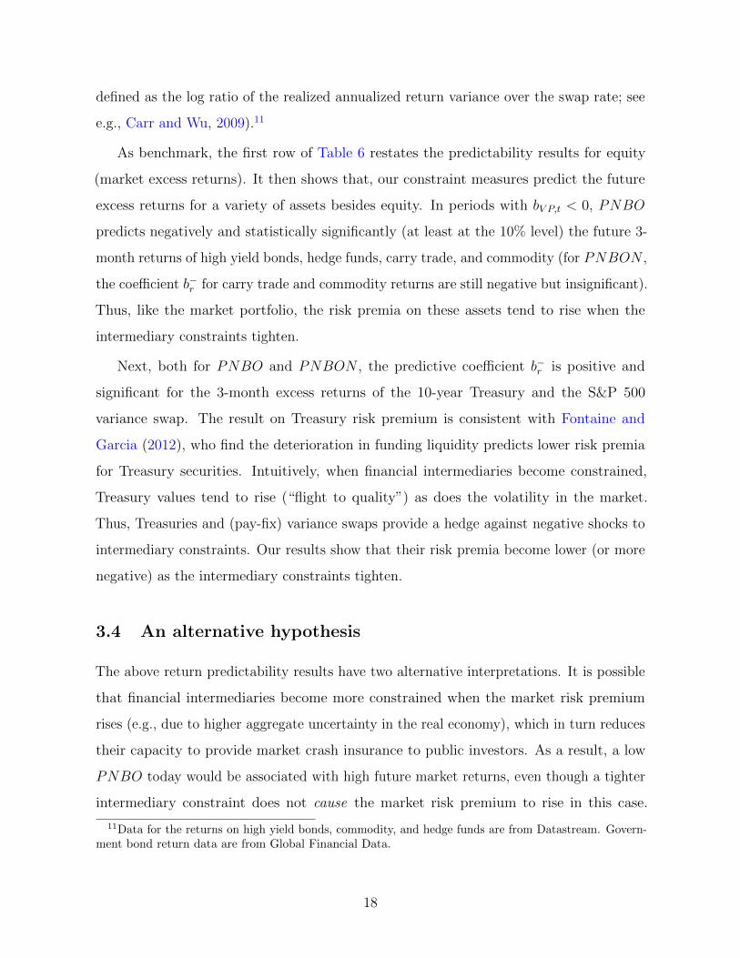
Next, both for PNBO and PNBON , the predictive coefficient b−r is positive and
significant for the 3-month excess returns of the 10-year Treasury and the S&P 500
variance swap. The result on Treasury risk premium is consistent with Fontaine and
Garcia (2012), who find the deterioration in funding liquidity predicts lower risk premia
for Treasury securities. Intuitively, when financial intermediaries become constrained,
Treasury values tend to rise (“flight to quality”) as does the volatility in the market.
Thus, Treasuries and (pay-fix) variance swaps provide a hedge against negative shocks to
intermediary constraints. Our results show that their risk premia become lower (or more
negative) as the intermediary constraints tighten.
3.4 An alternative hypothesis
The above return predictability results have two alternative interpretations. It is possible
that financial intermediaries become more constrained when the market risk premium
rises (e.g., due to higher aggregate uncertainty in the real economy), which in turn reduces
their capacity to provide market crash insurance to public investors. As a result, a low
PNBO today would be associated with high future market returns, even though a tighter
intermediary constraint does not cause the market risk premium to rise in this case.
11Data for the returns on high yield bonds, commodity, and hedge funds are from Datastream. Govern-ment bond return data are from Global Financial Data.
18
Alternatively, it is possible that intermediary constraints directly affect the aggregate
market risk premium, which is a central prediction in intermediary asset pricing theories.
To distinguish between these two interpretations, we compare PNBO against a number
of financial and macro variables that have been shown to predict market returns. If PNBO
is merely correlated with the standard risk factors and does not directly affect the risk
premium, then the inclusion of the proper risk factors into the predictability regression
should drive away the predictive power of PNBO. The variables we consider include the
difference between implied and historical volatility used in Bollerslev, Tauchen, and Zhou
(2009) (IV RV ), the log dividend yield (d− p) of the market portfolio, the log net payout
yield (lcrspnpy) by Boudoukh, Michaely, Richardson, and Roberts (2007), the Baa-Aaa
credit spread (DEF), the 10-year minus 3-month Treasury term spread (TERM), the tail
risk measure (Tail) by Kelly (2012), the slope of the implied volatility curve (IVSlope),
and the consumption-wealth ratio measure (cay) by Lettau and Ludvigson (2001). All the
variables are available monthly except for cay, which is at quarterly frequency.
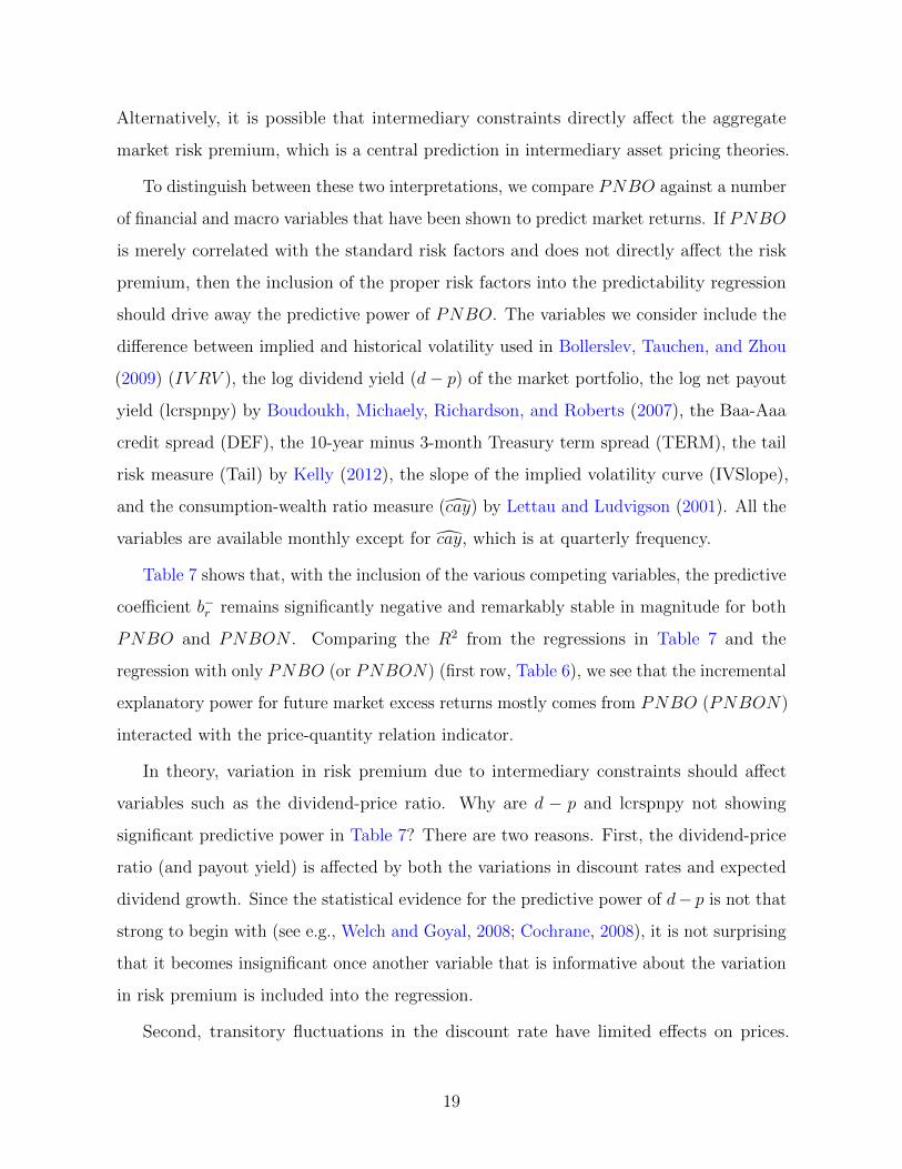
Table 7 shows that, with the inclusion of the various competing variables, the predictive
coefficient b−r remains significantly negative and remarkably stable in magnitude for both
PNBO and PNBON . Comparing the R2 from the regressions in Table 7 and the
regression with only PNBO (or PNBON) (first row, Table 6), we see that the incremental
explanatory power for future market excess returns mostly comes from PNBO (PNBON)
interacted with the price-quantity relation indicator.
In theory, variation in risk premium due to intermediary constraints should affect
variables such as the dividend-price ratio. Why are d − p and lcrspnpy not showing
significant predictive power in Table 7? There are two reasons. First, the dividend-price
ratio (and payout yield) is affected by both the variations in discount rates and expected
dividend growth. Since the statistical evidence for the predictive power of d− p is not that
strong to begin with (see e.g., Welch and Goyal, 2008; Cochrane, 2008), it is not surprising
that it becomes insignificant once another variable that is informative about the variation
in risk premium is included into the regression.
Second, transitory fluctuations in the discount rate have limited effects on prices.
19

Instead, the dividend-price ratio should be more sensitive to changes in longer-term
discount rates. We find that the predictive power of PNBO lasts only for up to 4 months
into the future, which is consistent with the intuition that episodes of tight intermediary
constraints are likely to have temporary effects on the risk premium. In comparison,
evidence on the predictive power for dividend-price ratio and related measures in the
literature are typically at longer horizons.
In summary, the results from Table 7 show that the option trading activities of public
investors and financial intermediaries contain unique information about the market risk
premium that is not captured by the standard macro and financial factors. This result is
consistent with the theories of intermediary constraints driving asset prices. Of course,
the evidence above does not prove that intermediary constraints actually drive aggregate
risk premia. It is possible that PNBO is correlated with other risk factors not considered
in our specifications.
3.5 Option volume and measures of funding constraints
We have presented evidence linking PNBO negatively with option expensiveness and
market risk premium when IbV P,t<0, which is consistent with the interpretation that low
PNBO is a sign of tight intermediary constraints. Thus, IbV P,t<0 × PNBONt can be
viewed as a measure of intermediary constraint. We now compare this measure to several
measures of financial intermediary funding constraints proposed in the literature.
These measures include the year-over-year change in broker-dealer leverage advocated
by Adrian, Moench, and Shin (2010) (∆lev), the fixed-income market based funding
liquidity measure by Fontaine and Garcia (2012) (FG), the TED spread (TED, the
difference between 3-month LIBOR and 3-month T-bill rate), and the LIBOR-OIS spread
(LIBOR-OIS, the difference between 3-month LIBOR and 3-month overnight indexed swap
rate).12 TED spread and LIBOR-OIS spread measure the credit risk of banks.
We first run OLS regressions of our constraint measure on the funding constraint
12We also examine the funding constraint measure by Hu, Pan, and Wang (2013) and the CBOE VIXindex (VIX). Neither of them is statistically significantly related to PNBO.
20

measures in the literature. As Panel A of Table 8 shows, TED spread is significantly
positively related to IbV P,t<0 × PNBOt, but insignificantly related to IbV P,t<0 × PNBONt.
The positive relation between TED spread and IbV P,t<0 × PNBOt is mainly due to the
fact that PNBO rose significantly along with the TED spread during the early part of
the financial crisis. Subsequently, while PNBO becomes lower (and turned significantly
negative), the TED spread also fell and then remained at low levels. This result points
out a potential weakness of the TED spread (and LIBOR-OIS) as a measure of funding
constraint. The TED spread could become lower because of the cautionary measures
banks take to reduce their own credit risk, which includes aggressive deleveraging and
buying crash insurance, but they do not necessarily imply that banks are less constrained
(it could in fact be just the opposite).
Next, our constraint measure is significantly negatively related to the measure FG. This
is consistent with FG’s interpretation that financial intermediaries are more constrained
(low PNBO) in periods when the value of funding liquidity is high (high FG).
In the quarterly regression, IbV P,t<0 × PNBOt is significantly positively related to the
growth rate in broker-dealer leverage ∆lev. That is, intermediary constraint tends to
be tight (low PNBO) when broker-dealers are de-leveraging (low ∆lev). This finding is
consistent with models of pro-cyclical leverage (e.g., Adrian and Shin (2010)) but not for
models of counter-cyclical leverage (e.g., He and Krishnamurhty (2012)). The different
forces behind the changes in leverage could reconcile these two predictions. If a bank’s
leverage falls due to a positive shock to its asset value (as in He and Krishnamurhty
(2012)), then lower leverage will indeed indicate relaxation of funding constraints. However,
if a bank is forced to delever due to stricter banking regulation, then lower leverage could
indicate tightening of constraints.
In Panel B of Table 8, we further examine the ability of the various funding constraint
measures to predict aggregate market returns. Adrian, Moench, and Shin (2010) show
that ∆lev has strong predictive power for excess returns on stocks, corporate bonds, and
treasuries. In a univariate regression (unreported) with ∆lev, we find similar results in our
sample period. When joint with our constraint measure, the coefficient on ∆lev becomes
21

insignificant in the case of PNBO and marginally significant in the case of PNBON ,
while b−r remains significant. Similarly, when the other funding constraint measures are
used in place of ∆lev, the coefficient b−r is always highly significant. These results suggest
that relative to other funding constraint measures, our intermediary constraint measure
contains unique information about conditional market risk premia.
3.6 Econometric identification of supply shocks
Besides the identification of “supply environments” based on the price-quantity relation,
an alternative method to identify supply shocks would be econometric identification.
One method suited for our study is identification through heteroskedasticity of Rigobon
(2003).13 In this section, we first briefly review the methodology of Rigobon (2003). Then,
we apply it to our setting to econometrically extract supply shocks and investigate the
relationship between supply shocks and risk premia.
Rigobon (2003) considers a standard linear supply-demand relationship between prices
(pt) and quantities (qt):
pt = b+ βqt + εt, (demand equation) (5)
qt = a+ αpt + ηt, (supply equation) (6)
where the volatilities of the supply and demand shocks are σε and ση, respectively. In
general, the residuals will be correlated with the independent variables in each equation
and the parameters will not be identified. Rigobon (2003) solves this identification problem
by considering regime-dependent heteroskadasticty of (ε, η). Supposing that there are
two regimes and the relative volatilities of the supply and demand shocks vary across the
regimes, the supply and demand equations can be identified.
We implement this method using V P as the price variable and PNBO as the quantity
variable. Following Rigobon (2003) (who uses crisis periods in debt markets to identify
movement in bond markets in Latin America), we consider two regimes for our identification:
13We thank an anonymous referee for this suggestion.
22

the crisis period (December 2007 to May 2009) and non-crisis periods.14 From the estimated
parameters, we then extract a time series of supply shocks (η). The extracted supply
shock is strongly related to PNBO with a correlation of 0.80. As with PNBON , we also
form normalized supply shocks by deflating by 3-month trailing average SPX volume.
Table 9 reproduces the predictability results of Table 4 replacing PNBO and PNBON
with the extracted supply shocks and normalized supply shocks.15 Overall, the predictability
with the extracted shocks is very similar to what we found with PNBO and PNBON ,
which reinforces our interpretation of the results.
However, we temper this evidence with several caveats based on the assumptions of
the methodology and its application to our setting. The method used here to identify
supply shocks assumes purely linear and stationary supply/demand relationships, and
zero correlation between supply and demand shocks. One could easily imagine non-linear
relationships (such as a dependency on the level of jump risk) or slope coefficients that
vary with the volatility regime, as well as non-zero correlation between supply and demand
shocks due to exogenous factors simultaneously driving supply and demand. By imposing
additional assumptions, one could incorporate some of these factors into the estimation,
but such choices may be difficult to make.
3.7 Public investors: retail vs. institutional
As Figure 1 shows, while financial intermediaries typically sell DOTM SPX puts to public
investors during normal times, the roles are often reversed during crisis times, most notably
during the 2008-09 financial crisis. To understand the risk sharing mechanism between
financial intermediaries and public investors, it is informative to find out who among the
public investors are the “liquidity providers,” reducing the demand for crash insurance
14The estimation results are reported in Table IA3 of the Internet Appendix. In our estimation, wedeleted December 2012, which has a variance premium of 221, 9.3 standard deviations above the average;including this data point would result in an almost certainly counterfactual negative (though insignificantlydifferent from zero) supply slope. Extracting supply shocks with the full sample resulted in supply shocksthat were nearly perfectly correlated with PNBO.
15In the regression, we use the Hodrick (1992) standard errors to be consistent with the remainder ofthe paper, which do not correct for the error in variables associated with uncertainty in the parametersused to extract the supply shocks.
23

or even providing insurance to the intermediaries when the latter become constrained.
The SPX volume data from CBOE do not provide further information about the types of
public investors behind a given transaction (e.g., retail vs. institutional investors). We
tackle this question by comparing the trading activities of the public investors in SPX
options with those in SPY options.
While SPX and SPY options have essentially identical underlying asset, it is well
known among practitioners that institutional investors account for a significantly higher
percentage of the trading volume of SPX options than do SPY options. Compared to
retail investors, institutional investors prefer SPX options due to a larger contract size (10
times as large as SPY), cash settlement, more favorable tax treatment, as well as being
more capable of trading in between the relatively wide bid-ask spreads of SPX options
due to stronger bargaining power. We construct PNBOSPY for SPY options using the
same procedure as PNBO, which covers the period from 2005/05 to 2012/12. While SPX
options trade exclusively on the CBOE, SPY options are cross-listed at several option
exchanges. PNBOSPY aggregates the volume from the CBOE and International Securities
Exchange (ISE), which account for about half of the total trading volume for SPY options.
Figure 6 compares the PNBOSPY and PNBOSPX (equivalent to PNBO) series.
During the period of 2005/05 to 2012/01, PNBOSPY is positive in the majority of the
months. From 2008/09 to 2010/12, PNBOSPX is negative in 22 out of 28 months, whereas
PNBOSPY is negative in just 7 of the 28 months.
A systematic way to examine the difference in how the equilibrium quantities of
trading in the two markets are connected to the intermediary constraints and market risk
premium is through the regressions of (3) and (4). These results are reported in Table A2
in Appendix B. To summarize, unlike PNBOSPX , PNBOSPY is insignificantly (and
positively) related to the variance premium on average, and the predictive coefficient b−r
for PNBOSPY is insignificant in the period of 2005/05 to 2012/12 (with much smaller R2).
The fact that PNBOSPX and PNBOSPY behave so differently in relation to variations
in V P and market risk premium suggests that institutional investors and retail investors
respond differently to the changes in intermediary constraints.16 In particular, when
16This difference in public investor trading behaviors between the two markets does not necessarily
24
constrained financial intermediaries start buying crash insurance, they appear to be buying
the insurance from the public (institutional) investors in the SPX market and not from
the public (retail) investors in the SPY market.
4 Robustness Checks
In this section, we report the results of several robustness checks for our main results.
4.1 Financial crisis and outliers
One potential concern regarding the predictive power of PNBO is that it might be driven
by a small number of outliers, in particular those observations during the 2008-09 financial
crisis. To address this concern, we re-estimate the predictive regressions for 3-month
market excess returns after removing a certain number of the most extreme observations of
PNBO and PNBON (in terms of the absolute value). Figure 4 shows the 95% confidence
intervals of the b−r coefficient after the removal of the extreme observations. The predictive
coefficients have relatively stable point estimates and remain significantly negative even
after deleting up to 50 extreme observations (19% of the sample).
Table 10 reports the results of the return-forecasting regressions in two sub-samples:
pre-crisis (1991/01-2007/11) and post-crisis (2009/06-2012/12). The predictive powers of
PNBO and PNBON remain statistically significant in both sub-samples. The economic
significance of the predictive power is weaker in the pre-crisis period than in the full sample
(in terms of smaller magnitude of b−r and lower R2) than the full sample, but it is quite
strong in the post-crisis period. Thus, the predictive power of our measure of intermediary
constraint is not just a crisis phenomenon. The weaker predictive power for PNBO in the
earlier sample period could be due to the fact that intermediary constraints are not as
significant and volatile in the first half of the sample. Another reason might be that the
SPX options market was less developed in the early periods and did not play as important
a role in facilitating risk sharing as it does today.
imply arbitrage, since the same financial intermediaries are present in both markets.
25

4.2 Moneyness
Next, we examine how the predictive power of PNBO changes based on option moneyness.
Our baseline definition of DOTM puts uses a simple cutoff rule K/S ≤ 0.85. Panel A
of Figure 5 plots the coefficient b−r and the confidence intervals as we change this cutoff
value for SPX puts. The coefficient b−r in the return forecast regression is significantly
negative for a wide range of moneyness cutoffs. The point estimate of b−r does become
more negative as the cutoff becomes smaller. Because DOTM puts are more difficult to
hedge than ATM puts, they expose financial intermediaries to more inventory risks. Hence,
PNBO measure based on DOTM puts should be more informative about intermediary
constraints and in turn the aggregate risk premium than PNBO based on ATM puts. At
the same time, because far out-of-money options are less liquid, the PNBO series becomes
more noisy when we further reduce the cutoff, which widens the confidence interval on b−r .
In contrast, Panel B shows that for essentially all moneyness cutoffs, PNBO based on
SPX call options does not predict market returns.
A feature of our definition of DOTM puts above is that a constant strike-to-price cutoff
implies different actual moneyness (e.g., as measured by option delta) for options with
different maturities. A 15% drop in price over one month might seem very extreme in
calm periods, but it is more likely when market volatility is high. For this reason, we
also examine a maturity-adjusted moneyness definition. Specifically, we classify a put
option as DOTM when K/S ≤ 1 + kσt√T , where k is a constant, σt is the daily S&P
return volatility in the previous 30 trading days, and T is the days to maturity for the
option. This is similar to using option delta to define moneyness, but does not require
a particular pricing model to compute the delta. Panel C of Figure 5 shows that this
alternative classification of DOTM puts produces qualitatively similar results as our simple
cutoff rule. Panel D shows again that PNBO based on SPX calls and this alternative
moneyness cutoff does not predict returns.
26

4.3 Volume vs. open interest
In our construction of PNBO, we focus on the net amount of new DOTM index puts
that public investors buy in a period. An alternative way to gauge the economic exposure
for public investors and financial intermediaries is to examine the net open interest for
the two groups. Between new volume and open interest, which one better represents the
degree of intermediary constraints?
We use the volume-based measure in our main analysis for two reasons. First, when
financial intermediaries become constrained, it is easier (e.g., due to transaction costs) to
adjust the quantity of new DOTM puts traded than to make significant changes in their
established positions. That makes the volume-based measure potentially more sensitive
to changes in intermediary constraints than open interest-based measure. Second, taking
on an option position that is originally near the money but later becomes DOTM due to
market movements is different from taking on a new DOTM option. In the former case,
the intermediaries can put on hedges against tail risk over time (via OTC options, VIX
options etc.), which means these positions are less sensitive to changes in intermediary
constraints.
Nonetheless, we provide two robustness checks. First, we examine an alternative
measure based on the end-of-month public net open interest for DOTM SPX puts (PNOI).
The results are discussed below. Second, we construct a PNBO measure using only one-
month options, for which the monthly measures of net volume and open interest are
equivalent. We find that the main results hold for the measure based on short-dated
options (see Table IA4 in the Internet Appendix).
For the period of 1991 to 2001, we use daily long and short open interest provided by
CBOE to compute PNOI. CBOE stopped providing the open interest data after 2001.
Thus, from 2001 onward, we compute daily net open interest from the volume information
as follows:
NOIK,Td = NOIK,Td−1 + openBuyK,Td − openSellK,Td + closeBuyK,T
d − closeSellK,Td , (7)
27

where NOIK,Td is the public investor net open interest of options with strike price K and
maturity T on day d, openBuy is the public investor buying volume from initiating long
positions, openSell is the selling volume from initiating short, closeBuy is the buying
volume from closing existing short positions, and closeSell is the selling volume from closing
existing long positions. We then aggregate NOIK,Td to compute daily net open interest of
DOTM puts (PNOI). We also consider a normalized version of PNOI (PNOIN), which
is PNOI divided by the sum of public long and short open interest for all SPX options.
Table 1 shows that the end-of-month PNOI is around 29,000 contracts on average,
and PNOI has higher autocorrelation than PNBO. Table 11 shows that, like PNBO,
PNOI predicts future market excess returns negatively in the periods with bV P,t < 0, with
significant coefficient b−r up to 3 months in the future. The R2 of the regressions are also
similar to PNBO. Additional sub-sample results for PNOI are provided in Table IA5.
4.4 Comparison with GPP
Our results on the price-quantity relation in the DOTM SPX puts market is related to
Garleanu, Pedersen, and Poteshman (2009). However, our results differ from GPP in
several aspects. First, we have a longer sample period, from 1991 to 2012, while theirs is
from 1996 to 2001. Second, our PNBO measure uses contemporaneous public net-buying
volume, while GPP use public net open interest,17 which is the accumulation of past
net-buying volumes. Third, our PNBO measure focuses on DOTM SPX puts, whereas
GPP use options of all moneyness (which is similar to the sum of PNBO and PNBOND
in this regard). In this section, we first replicate the main results of GPP (in Table 2,
p4287), and then examine the differences between the two studies.
The dependent variable in Table 12, option expensiveness, is the same as the one used
in GPP Table 2, i.e., the average implied volatility of ATM options minus a reference
model-implied volatility used in Bates (2006).18 GPP regress the option expensiveness
on several measures of SPX non-market-maker demand pressure, including the equal-
17GPP aggregate the net demand of both public investors and firm investors, and refer to it as thenon-market-maker demand.
18We thank David Bates for sharing the data on this measure.
28

weighted public open interest (NetDemand), and public open interest weighted by jump
risk (JumpRisk). They find the regression coefficients to be positive in the period from
1997/10 to 2001/12.
In Table 12, we obtain very similar results to GPP for the two sub-samples 1996/01-
1996/10 and 1997/10-2001/12 for the open interest-based measures. We also construct
two net volume-based measures and again find that they are positively related to option
expensiveness in the period from 1997/10 to 2001/12.
Next, for the period 2002-2012, we use daily volume data to extend the net open
interest measures (constructed using the procedure described in Section 4.3). In this
subsample, We find that the coefficients on both the open interest and volume-based
measures become negative and statistically significant. This finding is consistent with our
finding of a negative price-quantity relation in the full sample (see Table 3). The changing
signs of the price-quantity relation in different sub-samples suggest that the effects of
demand shocks and supply shocks are both present in the SPX option market.
5 Conclusion
We provide evidence that the trading activities of financial intermediaries in the market
of DOTM SPX put options are informative about the degree of intermediary constraints.
In periods when supply shocks are likely to be the main force behind the variations in
the price-quantity relation in the DOTM SPX put market, our public investor net-buying
volume measure, PNBO, has strong predictive power for future market excess returns
and the returns for a range of other financial assets. The predictive power of PNBO is
stronger during periods when the market jump risk is high, and it is stronger for DOTM
puts. PNBO is also associated with several funding liquidity measures in the literature.
Moreover, the information that PNBO contains about the market risk premium is not
captured by the standard financial and macro variables. These results suggest that time-
varying intermediary constraints are driving the supply of crash insurance by financial
intermediaries and the risk premia in financial markets.
29

To explain these findings, we build a general equilibrium model of the crash insurance
market, which captures the time-varying intermediary constraints in reduced form. For
future work, further investigation of the sources of the variation in intermediary constraints,
both theoretically and empirically, will help us better understand how intermediary
constraints affect the financial markets.
30
Appendix
A A Dynamic Model
In Section 3, we present empirical evidence connecting the trading activities in the market
for DOTM SPX puts to option pricing, market risk premium, and various measures of
intermediary constraints. In particular, there is time-varying equilibrium demand for crash
insurance from public investors. The equilibrium demand is inversely related to the relative
price of DOTM put options—times in which the equilibrium demand is low are generally
times when the protection is very expensive. The demand for crash insurance is also
informative about future stock market returns over and above the information in standard
macro and financial variables. Finally, the demand for crash insurance is positively related
to the changes in broker-dealer leverage. We now examine an equilibrium model consistent
with these empirical facts.
A.1 Model setup
We consider an aggregate endowment in the economy which follows a jump diffusion
process where the endowment is subject to both a diffusive risk and a jump risk. In
particular, sudden severe drops in the aggregate endowment are a source of disaster risk
in this economy. There are two types of agents in the economy: small public investors
and competitive dealers. We assume there exists a representative public investor, who
is denoted by agent P , and a representative dealer, denoted by agent D. To induce
the two types of agents to trade, we assume that they have different beliefs about the
probability of disasters. Such differences in beliefs capture in reduced form the advantages
that dealers have in bearing disaster risk, whether it is due to differences in technology,
agency problems, or behavioral biases.19
Specifically, we assume that both agents believe that the log aggregate endowment,
ct = logCt, follows the process
dct = gdt+ σcdWct − d dNt, (A1)
where g and σc are the expected growth rate and volatility of consumption without jumps,
W ct is a standard Brownian motion under both agents’ beliefs, and d is the constant size
19Examples include government guarantees to large financial institutions and compensation schemesthat encourages managers to take on tail risk. See e.g., Lo (2001) and Malliaris and Yan (2010).
31

of consumption drop in a diaster20. Nt is a counting process whose jumps arrive with
stochastic intensity λt under the public investors’ beliefs, and λt follows
dλt = κ(λ− λt)dt+ σλ√λtdW
λt , (A2)
where λ is the long-run average jump intensity under P ’s beliefs, and W λt is a standard
Brownian motion independent of W ct . In general, the dealers are more willing to bear
the disaster risk because (they act as if) they are more optimistic about disaster risk.
We assume that they believe that the disaster intensity is given by ρλt with ρ < 1. We
summarize the public investors’ beliefs with the probability measure PP , and the dealers’
beliefs with the probability measure PD.
Public investors have standard constant relative risk aversion (CRRA) utility:
UP = EP0
[∫ ∞0
e−δtC1−γP,t
1− γdt
], (A3)
where we focus on the cases where γ > 1. The superscript P reflects that the expectations
are taken under the public investors’ beliefs.
The utility function of the dealers are different. We assume that the dealers face an
intermediation constraint that we model in a reduced form directly in terms of their utility.
Specifically, we suppose that
UD = ED0
[∫ ∞0
e−δtC1−γD,t
1− γe−
∑Ntn=1(ατ(n)−α)dt
], (A4)
where αt is a stochastic variable representing the ability of the dealer to intermediate
disaster risk. Limited ability to intermediate risk is modeled as increased risk aversion
against market crashes. This specification generalizes the state-dependent preferences
proposed by Bates (2008) in that it allows the dealers’ risk aversion against crashes to rise
with the probability of disasters.
Specifically, τ(n) is the time of the nth disaster since t = 0, τ(n) ≡ inf{s : Ns = n}Thus, this crash-aversion term remains constant in between disasters. Suppose the dealer’s
log consumption drops by dD,τ(n) at the time of the nth disaster. Then, at the same time,
the marginal utility of the dealer jumps up by
eγdD,τ(n)−(ατ(n)−α) = e
(γ−
ατ(n)−α)
dD,τ(n)
)dD,τ(n)
, (A5)
20As in Chen, Joslin, and Tran (2012), one could generalize the model by allowing disaster size to havea time-invariant distribution.
32

which implies that the dealer’s effective relative risk aversion against the disaster is
γD,τ(n) = γ −ατ(n) − αdD,τ(n)
. (A6)
Thus, when αt > α, the dealer will have lower aversion to disaster risk than the public
investor. As αt falls, the dealer’s effective risk aversion rises.
The intermediation capacity of the dealer may be related to the disaster intensity.
We model the intermediation as being driven jointly by the disaster intensity, λt, and an
independent factor, xt, so that αt = −aλt + bxt. Thus when a > 0, the intermediation
capacity goes down as the intensity rises and the dealer becomes more averse to disaster
risk.
Any jointly affine process for (ct, λt, xt) would be suitable for a tractable specification.
For example, we could suppose that xt follows an independent CIR process:
dxt = κx(x− xt)dt+ σx√xtdW
xt . (A7)
In our calibrations, we will choose the simple specification with b = 0 so that the
intermediation capacity is perfectly correlated with the disaster intensity.
The main motivation for the dealer’s time-varying aversion to crash risk is the time-
varying constraint faced by financial intermediaries. Rising crash risk in the economy
raises the intermediaries’ capital/collateral requirements and tightens their constraints
on tail risk exposures (e.g., Value-at-Risk constraints), which make them more reluctant
to provide insurance against disaster risk. For example, see Adrian and Shin (2010) and
He and Krishnamurhty (2012). In this sense, the shocks to the disaster intensity in the
model also serve the purpose of generating time variation in the intermediation capacity
of the dealer. We can further generalize the specification by making the dealer’s aversion
to crash risk driven by adding independent variations in the intermediation shocks.
We also assume that markets are complete and agents are endowed with some fixed
share of aggregate consumption (θP , θD = 1 − θP ). The equilibrium allocations can
be characterized as the solution of the following planner’s problem, specified under the
probability measure PP ,
maxCPt , C
Pt
EP0
[∫ ∞0
e−δt(CP
t )1−γ
1− γ+ ζηte
−δt (CDt )1−γea
∑Ntn=1(λτ(n)−λ)
1− γdt
], (A8)
subject to the resource constraint CPt + CD
t = Ct. Here, ζ is the the Pareto weight for the
33

dealers and
ηt ≡dPDdPP
= ρNte(1−ρ)∫ t0 λsds. (A9)
where ρ = λD/λ, the relative likelihood of a jump under the two beliefs. From the
first order condition and the resource constraint, we obtain the equilibrium consumption
allocations CPt = fP (ζt)Ct and CD
t = (1− fP (ζt))Ct, where
ζt = ρNt e(1−ρ)
∫ t0 λsds+α
∑Ntn=1(λτ(n)−λ)ζ (A10)
and
fP (ζ) =1
1 + ζ1γ
. (A11)
The stochastic discount factor under P ’s beliefs, MPt , is given by
MPt = e−ρt(CP
t )−γ = e−δtfP (ζt)−γC−γt . (A12)
We can solve for the Pareto weight ζ through the lifetime budget constraint for one of the
agents (Cox and Huang (1989)), which is linked to the initial allocation of endowments.
Our key focus will be on risk premiums and on the net public purchase of crash
insurance which we relate to the market for deep out of the money puts in our empirical
analysis. The risk premium for any security under each agent’s beliefs is the difference
between the expected return under Pi and under the risk-neutral measure Q.
Eit [R
e] = γσc∂BP + (λit − λQt )Ed
t [R], i = D,P, (A13)
where we use the shorthand that ∂BP denotes the sensitivity of the security to Brownian
shocks and Edt [R] is the expected return of the security conditional on a disaster. Since
consumption will be relatively smooth in our calibration, the return of securities which
are not highly levered on the Brownian risk will be dominated by the jump risk term.
Moreover, agents agree about the Brownian risk and have the same risk aversion with
respect to these shocks so there will be no variation in the Sharpe ratio for Brownian risk.
In light of these facts, we focus on the variation in the jump risk premium, as measured
by λQ/λPP .
The stochastic discount factor characterizes the unique risk neutral probability measure
Q. The risk-neutral disaster intensity, λQt ≡ Edt [M i
t ]/Mitλ
it, is determined by the expected
jump size of the stochastic discount factor at the time of a disaster. When the risk-free
rate and disaster intensity are close to zero, the risk-neutral disaster intensity has the
nice interpretation of (approximately) the value of a one-year crash insurance contract
34

that pays one at t + 1 when a disaster occurs between t and t + 1. In our setting, the
risk-neutral jump intensity is given by
λQt = eγd(1 + (ρζt)
1γ)γ
(1 + ζ1γ
t )γλt. (A14)
In order to define the market size, we must consider how the Pareto efficient allocation
is obtained. The equilibrium allocations can be implemented through competitive trading
in a sequential-trade economy. Extending the analysis of Bates (2008), we can consider
four types of traded securities: (i) a risk-free money market account, (ii) a claim to
aggregate consumption, and (iii) a crash insurance contracts which pays one dollar in the
event of a disaster in exchange for a continuous premium, and (iv) a separate instrument
sensitive only to shocks in the disaster intensity. As in Chen, Joslin, and Tran (2012),
since agents agree about the Brownian risk and have identical aversion to the risk, they
will proportionally hold the Brownian risk according to their consumption share. With the
instruments we have specified, this means they will proportionally hold the consumption
claim. Thus, the agents will hold proportional exposure to the disaster risk from their
exposure to the consumption claim. Motivated by these facts, we define the net public
purchase for crash insurance as the (scaled) difference between the consumption loss
the public bears in equilibrium minus the consumption loss that the public would bear
without insurance. That is, the public purchase for insurance is the difference between
e−d(fP (ζdt ) − fP (ζt−)) (where ζdt is the value of ζt conditional on a disaster occurring
at time t: ζdt = ρeα(λt−−λ)ζt−) and e−d(fP (ζdt )− fP (ζt−). Thus we define the net public
purchase for insurance as
net public purchase for crash insurance = e−d(fP (ζtρe
α(λt−−λ))− fP (ζt)). (A15)
A.2 Net public purchase and risk premia in the dynamic model
We now study the relationship between public purchase and risk premia in the context
of our dynamic model. We calibrate our model as in Chen, Joslin, and Tran (2012)
and Wachter (2013). The key new parameter that we introduce is the time-variation in
aversion to jump risk. We parameterize this by setting a = αd/σSS(λ), where σSS(λ) is
the volatility of the stationary distribution of λ. We choose α = 1, which together with
the other parameters implies that when λ = 2.35% (one standard deviation from the
steady state volatility (65 bp) above the long run mean (1.7%)), an economy populated
by only the dealer will behave as an economy with a representative agent with relative
risk aversion of 5 with respect to jumps (one higher than if he had standard CRRA utility
35

with γ = 4). As a baseline comparison, we also consider the parameterization with α = 0,
which corresponds to the stochastic intensity model of Chen, Joslin, and Tran (2012).
In our model, there are two state variable: λt, the likelihood of a disaster, and ft, the
public investors consumption share. Figure A1 plots the net public purchase of crash
insurance as a function of the public consumption share and the jump intensity. When
α = 0 (panel B), the amount of risk sharing does not depend on λ as the motivation to
share risk depends only on the size of the jump in consumption. The equilibrium public
purchase is close to zero when either the public has a low consumption share (the public
has limited resources to buy insurance) or when the public has high consumption share
(the dealers have limited ability to provide insurance) with a peak in the middle where the
public and dealers share a lot of risk. In contrasts, Panel B shows that when the dealers
have time-varying aversion to jump risk, the relationship is much more complex. For low
levels of the intensity the patterns is the same as before since the dealers are as willing (or
even more willing) to sell crash insurance. However, as λ rises, the dealer becomes more
averse to jump risk and is less willing to provide insurance. When the intensity becomes
high enough, the dealers become so averse to jump risk that they even begin to become
buyers of insurance rather than sellers.
Figure A2 plots the jump risk premium, as measured by λQ/λ, as a function of the
public consumption share and the jump intensity. In the case of α = 0, the jump risk
premium rises as there are fewer dealers to hold the jump risk. When α = 1 and λ is
low, the jump risk premium falls as the dealer’s consumption share increases. When
λ is high enough, this relationship reverses and the premium rises as the dealer gains
consumption share. The reason for this is that as λ rises, the dealer becomes more risk
averse and eventually demands a higher premium than the public; this relation can be
seen be following the curve with ft = 0, corresponding to the case where there is only the
dealer.
Next, we examine the relation between the net public purchase of crash insurance
and the disaster risk premium in equilibrium. We do so by first holding constant the
consumption share of the public investors (ft) while letting the disaster intensity (λt) vary
over time. The results are in Figure A3. When α = 1, for each of the consumption shares
considered (ft = 0.9, 0.8, 0.5), the model predicts a negative relation between the net
public purchase for crash insurance and risk premium. This negative relation is consistent
with our empirical finding of bV P < 0 in Equation (3) and br < 0 in Equation (4).
In contrast, when α = 0, i.e., when the dealer has constant risk aversion for disaster
risk, both the net public purchase and the disaster risk premium remain constant as the
disaster intensity changes. This comparison again highlights the key role played by the
dealer’s time-varying aversion to disaster risk in our model.
36

When we fix the disaster intensity and let the consumption share vary over time, the
relation between the net public purchase of crash insurance and the disaster risk premium
is no longer monotonic. Consider first the case with α = 0, i.e., the case where the dealer
has constant relative risk aversion (see Panel B of Figure A4). In this case, regardless of the
disaster intensity, there is a unique relation between the two quantities: as consumption
share of the public investors changes from 0 to 1, the net public purchase, as defined
in (A15), starts at 0, reaches its peak at 11%, and then falls back to 0 eventually. The
limiting case where the public investor own all the aggregate endowment is marked by the
red circle on the y-axis. In this process, because the relative amount of risk sharing by the
public investor falls as he gains a larger share of consumption, the disaster risk premium
in equilibrium rises monotonically until it reaches the limit of eγd = 7.7.
Consider now the case where the dealer has time-varying risk aversion (α = 1). When
α = 1, (Panel A of Figure A4) the relation between the net public purchase of crash
insurance and the disaster risk premium is qualitatively similar to that in Panel B (where
α = 0) when the disaster intensity is not too high. The equilibrium where public investors
own all the endowment is still identical regardless of the level of disaster intensity (again
marked by the red circle), but the other extreme where the dealer owns all the endowment
has different risk premiums for different disaster intensities. This result is simply due to
the dealer’s time-varying risk aversion. When λt is sufficiently high, the dealer can become
so averse to disaster risk that, despite his optimist beliefs about the chances of disasters,
the dealer still demands a higher premium than the public investors would. For this reason,
when λt is sufficiently high, the net public purchase of crash insurance turns negative,
i.e., the public investor is now insuring the dealer against disasters, and the disaster risk
premium in the economy exceeds the highest level in the case with constant risk aversion.
Panel A of Figure A4 also illustrate that, as the level of disaster intensity λt rises, the
relation between the disaster risk premium and the net public purchase of crash insurance
becomes more negative in the region near the red circle. That is, when public investors
own the majority of the wealth in the economy, changes in the public demand for crash
insurance are accompanied by larger swings in aggregate risk premium when the level of
crash risk is higher. This prediction is confirmed by our empirical finding of cV P < 0 in
Equation (3).
Figure A5 examines the relationship between the dealer leverage and the consumption
share of the public investor and the disaster intensity. Here, we measure the leverage of
the dealers as the ratio of the equilibrium consumption loss of the dealers (which includes
losses from selling disaster insurance and their equity position) to their consumption loss
they would bear without selling any insurance. When the disaster probability is low, so
that the dealers are relatively unconstrained and aggressively sell insurance, the dealer
37

leverage increases to a maximum of around two when public investors own the majority of
the wealth. For a given level of disaster probability, the dealer leverage decreases as public
investors’ wealth (consumption) share becomes smaller. As the disaster probability rises,
the dealers become more constrained and begin to deleverage. In some cases, the dealer
leverage as we define may even fall below one, indicating that the dealers are acquiring
insurance to reduce their exposures to disaster risks.
Taken together, the results from Figure A1 and Figure A5 show that our model is
able to capture the negative relation between intermediary leverage growth and the net
quantity of trading in disaster insurance in the data, as documented in Table 8.
B Additional Empirical Results
Additional empirical results and robustness checks are provided in the Internet Appendix.
They include (1) a table of correlations between PNBO and various macroeconomic and
financial variables (Table IA1); (2) systematic analysis of the statistical significance for
the return-forecasting regressions using PBNO and PNBON (Table IA2); (3) parameter
estimates from estimation of the supply-demand system using the method of Rigobon (2003)
(Table IA3); (4) return-forecasting regression with PNBO1month (and PNBON1month),
which is PNBO constructed using only options with one month or less to maturity (Table
IA4); (5) sub-sample return-forecasting regressions with PNOI (Table IA5); (6) return-
forecasting regression with PNB (and PNBN), which is the public net buy volume for
DOTM SPX puts including both open and close transactions (Table IA6); (7) return-
forecasting regression using a modified CDM method (Table IA7); (8) return-forecasting
regression using bV P + cV PJt as indicator (Table IA8); (9) sub-sample return-forecasting
regressions with the log dividend-price ratio (Table IA9).
38

References
Adrian, Tobias, and Nina Boyarchenko, 2012, Intermediary leverage cycles and financialstability, Staff reports, Federal Reserve Bank of New York.
Adrian, Tobias, Erkko Etula, and Tyler Muir, 2012, Financial intermediaries and thecross-section of asset returns, Working Paper.
Adrian, Tobias, Emanuel Moench, and Hyun Song Shin, 2010, Financial intermediation,asset prices, and macroeconomic dynamics, Staff Reports 422 Federal Reserve Bank ofNew York.
Adrian, Tobias, and Hyun Song Shin, 2010, Liquidity and leverage, Journal of FinancialIntermediation 19, 418–437.
Andersen, T. G., T. Bollerslev, and F. X. Diebold, 2007, Roughing it up: Including jumpcomponents in the measurement, modeling, and forecasting of return volatility, Reviewof Economics and Statistics 89, 701–720.
Ang, Andrew, and Geert Bekaert, 2007, Stock return predictability: Is it there?, Reviewof Financial Studies 20, 651–707.
Bates, David S., 2006, Maximum Likelihood Estimation of Latent Affine Processes, Reviewof Financial Studies 19, 909–965.
, 2008, The market for crash risk, Journal of Economic Dynamics and Control 32.
Bekaert, Geert, and Marie Hoerova, 2014, The VIX, the variance premium and stockmarket volatility, Journal of Econometrics 183, 181–192.
Bernanke, Ben, and Mark Gertler, 1989, Agency Costs, Net Worth, and Business Fluctua-tions, American Economic Review 79, 14–31.
Bernanke, Ben S., Mark Gertler, and Simon Gilchrist, 1999, The financial accelerator in aquantitative business cycle framework, in J. B. Taylor, and M. Woodford, ed.: Handbookof Macroeconomics, vol. 1 of Handbook of Macroeconomics . chap. 21, pp. 1341–1393(Elsevier).
Bollen, Nicolas, and Robert Whaley, 2004, Does net buying pressure affect the shape ofimplied volatility functions?, Journal of Finance 59, 711–753.
Bollerslev, Tim, George Tauchen, and Hao Zhou, 2009, Expected stock returns and variancerisk premia, Review of Financial Studies 22, 4463–4492.
Boudoukh, Jacob, Roni Michaely, Matthew Richardson, and Michael R. Roberts, 2007, Onthe Importance of Measuring Payout Yield: Implications for Empirical Asset Pricing,Journal of Finance 62, 877–915.
Brunnermeier, Markus K., and Lasse Heje Pedersen, 2009, Market liquidity and fundingliquidity, Review of Financial Studies 22, 2201–2238.
39

Brunnermeier, Markus K., and Yuliy Sannikov, 2013, A macroeconomic model with afinancial sector, Working Paper, Princeton University.
Buraschi, Andrea, and Alexei Jiltsov, 2006, Model uncertainty and option markets withheterogeneous beliefs, Journal of Finance 61, 2841–2897.
Carr, Peter, and Liuren Wu, 2009, Variance risk premiums, Review of Financial Studies22, 1311–1341.
Chen, Hui, Scott Joslin, and Ngoc-Khanh Tran, 2012, Rare disasters and risk sharing withheterogeneous beliefs, Review of Financial Studies 25, 2189–2224.
Cochrane, John H., 1999, Portfolio advice of a multifactor world, Economic Perspectivespp. 59–78.
, 2008, The Dog That Did Not Bark: A Defense of Return Predictability, Reviewof Financial Studies 21, 1533–1575.
Cohen, Lauren, Karl B. Diether, and Christopher J. Malloy, 2007, Supply and DemandShifts in the Shorting Market, Journal of Finance 62, 2061–2096.
Cox, John C., and Chifu Huang, 1989, Optimum consumption and portfolio policies whenasset prices follow a diffusion process, Journal of Economic Theory 49, 33–83.
Fontaine, Jean-Sebastien, and Rene Garcia, 2012, Bond Liquidity Premia, Review ofFinancial Studies 25, 1207–1254.
Garleanu, Nicolae, Lasse Heje Pedersen, and Allen M. Poteshman, 2009, Demand-basedoption pricing, Review of Financial Studies 22, 4259–4299.
Geanakoplos, John, 2009, The leverage cycle, Cowles Foundation Discussion Papers 1715Cowles Foundation for Research in Economics, Yale University.
Gromb, Denis, and Dimitri Vayanos, 2002, Equilibrium and welfare in markets withfinancially constrained arbitrageurs, Journal of Financial Economics 66, 361–407.
Hansen, P.R., and A. Timmermann, 2012, Choice of sample split in out-of-sample forecastevaluation, Working Paper, Stanford University.
He, Zhiguo, and Arvind Krishnamurhty, 2012, Intermediary asset pricing, Forthcoming,American Economic Review.
Hodrick, RJ, 1992, Dividend yields and expected stock returns: alternative procedures forinference and measurement, Review of Financial Studies 5, 357–386.
Hu, Grace Xing, Jun Pan, and Jiang Wang, 2013, Noise as Information for Illiquidity,Journal of Finance 68, 2341–2382.
Johnson, Timothy C., Mo Liang, and Yun Liu, 2014, What drives index options exposure?,Working Paper.
40
Kelly, Bryan, 2012, Tail risk and asset prices, Working Paper, University of Chicago BoothSchool of Business.
Kiyotaki, Nobuhiro, and John Moore, 1997, Credit Cycles, Journal of Political Economy105, 211–48.
Lettau, Martin, and Sydney Ludvigson, 2001, Resurrecting the (C)CAPM: a cross-sectionaltest when risk premia are time-varying, Journal of Political Economy 109, 1238–1287.
Lo, Andrew, 2001, Risk management for hedge funds: Introduction and overview, FinancialAnalysts Journal 57, 16–33.
Longstaff, Francis A., and Jiang Wang, 2012, Asset pricing and the credit market, Reviewof Financial Studies 25, 3169–3215.
Lustig, Hanno, Nikolai Roussanov, and Adrien Verdelhan, 2011, Common Risk Factors inCurrency Markets, Review of Financial Studies 24, 3731–3777.
Malliaris, Steven, and Hongjun Yan, 2010, Reputation Concerns and Slow-Moving Capital,Working Paper, Yale University.
McCracken, Michael W., 2007, Asymptotics for out of sample tests of Granger causality,Journal of Econometrics 140, 719–752.
Muller, Ulrich K., 2014, Hac corrections for strongly autocorrelated time series, Journalof Business & Economic Statistics 32, 311–322.
Newey, W. K., and K. D. West, 1987, A simple positive semi-definite, heteroskedasticityand autocorrelation consistent covariance matrix estimator, Econometrica 55, 703–708.
Pan, Jun, and Allen Poteshman, 2006, The information in option volume for future stockprices, Review of Financial Studies 19, 871–908.
Rigobon, R, 2003, Identification through heteroskedasticity, Review of Economics andStatistics 85, 777–792.
Sentana, Enrique, and Gabriele Fiorentini, 2001, Identification, estimation and testing ofconditionally heteroskedastic factor models, Journal of Econometrics 102, 143–164.
Wachter, Jessica A., 2013, Can Time-Varying Risk of Rare Disasters Explain AggregateStock Market Volatility?, Journal of Finance 68, 987–1035.
Welch, Ivo, and Amit Goyal, 2008, A comprehensive look at the empirical performance ofequity premium prediction, Review of Financial Studies 21, 1455–1508.
41

Jan1995 Jan2000 Jan2005 Jan2010−3
−2
−1
0
1
2
3x 10
5 PNBO
Number
ofcontracts
Jan1995 Jan2000 Jan2005 Jan2010−0.03
−0.02
−0.01
0
0.01
0.02
0.03
0.04PNBON
Asian
Russian
Iraq War QuantBear Sterns
Lehman
TARP
TALF1
BoA
TALF2
Euro
GB1
EFSF
GB2
Voluntary
Referendum
AsianRussian
Iraq War
QuantBear Sterns
Lehman
TARP
TALF1
BoA
TALF2Euro
GB1
EFSF
GB2
Voluntary
Referendum
Figure 1: Time Series of net public purchase for DOTM SPX puts. PNBO is the netamount of deep-out-of-the-money (DOTM )(with K/S ≤ 0.85) SPX puts public investors buying-to-openeach month. PNBON is PNBO normalized by average of previous 3-month total volume from publicinvestors.“Asian” (1997/10): period around the Asian financial crisis. “Russian” (1998/11): period aroundRussian default. “Iraq” (2003/04): start of the Iraq War. “Quant” (2007/08): the crisis of quant-strategyhedge funds. “Bear Sterns” (2008/03): acquisition of Bear Sterns by JPMorgan. “Lehman” (2008/09):Lehman bankruptcy. “TARP” (2008/10): establishment of TARP. “TALF1” (2008/11): creation ofTALF. “BoA” (2009/01): Treasury, Fed, and FDIC assistance to Bank of America. “TALF2” (2009/02):increase of TALF to $1 trillion. “Euro” (2009/12): escalation of Greek debt crisis. “GB1” (2010/04):Greece seeks financial support from euro and IMF. “EFSF” (2010/05): establishment of EFSM and EFSF;110 billion bailout package to Greece agreed. “GB2” (2010/09): a second Greek bailout installment.“Voluntary” (2011/06): Merkel agrees to voluntary Greece bondholder role. “Referendum” (2011/10):further escalation of Euro debt crisis with the call for a Greek referendum.
42

below 0.85 [0.85 0.95] [0.95 0.99] [0.99 1.01] [1.01 1.05] [1.05 1.10] above 1.100
5
10
15
20
25
30
K/S
%
Percentage of Puts Volumes
below 0.85 [0.85 0.95] [0.95 0.99] [0.99 1.01] [1.01 1.05] [1.05 1.10] above 1.100
5
10
15
20
25
30
35
K/S
%
Percentage of Call Volumes
publicfirm
publicfirm
Figure 2: Percentage of total put and call volumes at different moneyness. Thisfigure plots the total fraction of volume for calls and puts at different levels of moneyness(measure by strike price, K, divided by spot price S). The height of each bar indicatesthe fraction of the total market volume at that moneyness level, while the colors indicatethe breakdown within the strike between public (blue) and private (red) orders.
43

Start of Evaluation Period1996 1998 2000 2002 2004 2006 2008
R2(%
)
0
5
10
15
20
25
30A. Out-of-Sample R2
PNBOPNBON
End of 5-year Window1996 2000 2004 2008 2012
R2(%
)
0
10
20
30
40
50
60B. 5-Year Moving-Window R2
PNBOPNBON
Figure 3: Out-of-sample R2 and R2 from 5-year moving-window regressions.This figures plots the out-of-sample R2 and R2 of 5-year moving windows from forecasting3-month market excess returns based on the specification of (4). Panel A plots the out-of-sample R2 as a function of the sample split date. Panel B plots the in-sample R2 as afunction of the end of 5-year moving windows.
44

No. of extreme obs deleted0 10 20 30 40 50
b! r
-200
-150
-100
-50
0A. PNBO
No. of extreme obs deleted0 10 20 30 40 50
b! r
-7
-6
-5
-4
-3
-2
-1
0B. PNBON
Figure 4: Predictability of PNBO and PNBON after deleting extreme observa-tions. This figures plots point estimates and 95% confidence intervals (based on Hodrick (1992)
standard errors) for the coefficient b−r from regression (4) forecasting 3-month market excess
returns, after removing various numbers of extreme PNBO observations.
45

K/S ≤ k0.75 0.8 0.85 0.9 0.95 1 1.05
b− r
-300
-250
-200
-150
-100
-50
0A. Puts
b−r95% C.I.
K/S ≤ k0.75 0.8 0.85 0.9 0.95 1 1.05
-300
-200
-100
0
100
200
300B. Calls
K/S ≤ 1 + kσ-2 -1.5 -1 -0.5 0 0.5
b− r
-80
-60
-40
-20
0C. Puts
K/S ≤ 1 + kσ-2 -1.5 -1 -0.5 0 0.5
-200
-100
0
100
200D. Calls
Figure 5: Predictive power of PNBO at different moneyness. This figure plots thepoint estimate and 95% confidence interval (based on Hodrick (1992) standard errors)for the coefficient b−r from regression (4) forecasting 3-month market excess returns. InPanels A and B, option moneyness is measured by the level of strike-to-price ratio K/S.In Panels C and D, option moneyness is measured by K/S relative to daily volatility ofS&P returns scaled by the square root of days to maturity (see Section 4.2).
46

2005 2006 2007 2008 2009 2010 2011 2012 2013
Num
ber
ofco
ntra
cts
#105
-3
-2
-1
0
1
2
3
4
PNBOSPX
PNBOSPY
Figure 6: Comparing PNBO for SPX and SPY options. This figure plots the publicnet buying-to-open volume for deep-out-of-the-money (with K/S ≤ 0.85) puts in themarket for SPX options and SPY options for the period of 2005/05 to 2012/12.
47

00.03
0.060
0.51
−0.05
0
0.05
0.1
0.15
λt
A. α = 1
ft
net
publicdem
and
00.03
0.060
0.51
−0.05
0
0.05
0.1
0.15
λt
B. α = 0
ft
net
publicdem
and
Figure A1: Net Public Purchase for Crash Insurance. The two panels plot the
net public purchase for crash insurance as a function of the public investor P’s consumption
share (ft) and the disaster intensity under P’s beliefs (λt). Panel A considers the case when
α = 1, which implies that a 1-standard deviation increase in the disaster intensity from its
long-run mean effectively increases the dealers’ relative risk aversion against disasters by 1 in the
homogeneous-agent economy. Panel B considers the case when α = 0.
48

0
0.03
0.06
0
0.5
10
10
20
30
λt
A. α = 1
ft
λQ t/λ
t
0
0.03
0.06
0
0.5
10
2
4
6
8
λt
B. α = 0
ft
λQ t/λ
t
Figure A2: Disaster Risk Premium. The two panels plot the conditional disaster risk
premium as a function of the public investor P’s consumption share (ft) and the disaster intensity
under P’s beliefs (λt). Panel A considers the case when α = 1. Panel B considers the case when
α = 0. Again, α = 1 means that a 1-standard deviation increase in the disaster intensity from its
long-run mean effectively increases the dealers’ relative risk aversion against disasters by 1 in the
homogeneous-agent economy.
49

−0.05 0 0.05 0.1 0.150
2
4
6
8
10
12
14
16
net public demand
λQ t/λ
t
A. α = 1
ft = 0.9ft = 0.8ft = 0.5
0.02 0.04 0.06 0.08 0.1 0.122
2.5
3
3.5
4
4.5
5
5.5
6
6.5
net public demand
λQ t/λ
t
B. α = 0
ft = 0.9ft = 0.8ft = 0.5
Figure A3: Net Public Purchase for Crash Insurance and Risk Premium: FixedConsumption Share. The two panels plot the conditional disaster risk premium against the
net public purchase for crash insurance while holding the public investors’ consumption share ftconstant. Panel A considers the case when α = 1. Panel B considers the case when α = 0.
50

−0.05 0 0.05 0.1 0.150
2
4
6
8
10
12
14
net public demand
λQ t/λ
t
A. α = 1
λ = 1.0%λ = 1.7%λ = 4.0%λ = 6.0%
0 0.05 0.1 0.150
1
2
3
4
5
6
7
8
net public demand
λQ t/λ
t
B. α = 0
λ = 1.0%λ = 1.7%λ = 4.0%λ = 6.0%
Figure A4: Net Public Purchase for Crash Insurance and Risk Premium: FixedDisaster Intensity. The two panels plot the conditional disaster risk premium against the
net public purchase for crash insurance while holding the disaster intensity λt constant. Panel A
considers the case when α = 1. Panel B considers the case when α = 0. The red circles mark the
limiting cases in the two economies where public investors own all the aggregate endowment.
51

00.01
0.020.03
0.040.05
0.060.07
0
0.2
0.4
0.6
0.8
1
0.4
0.6
0.8
1
1.2
1.4
1.6
1.8
2
λpublic consumption fraction
De
ale
r L
eve
rag
e
Figure A5: Dealer leverage. This figure plots the dealer leverage as a function of the public
consumption fraction and the disaster probability.
52
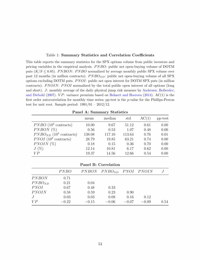
Table 1: Summary Statistics and Correlation Coefficients
This table reports the summary statistics for the SPX options volume from public investors and
pricing variables in the empirical analysis. PNBO: public net open-buying volume of DOTM
puts (K/S ≤ 0.85). PNBON : PNBO normalized by average monthly public SPX volume over
past 12 months (in million contracts). PNBOND: public net open-buying volume of all SPX
options excluding DOTM puts. PNOI: public net open interest for DOTM SPX puts (in million
contracts). PNOIN : PNOI normalized by the total public open interest of all options (long
and short). J : monthly average of the daily physical jump risk measure by Andersen, Bollerslev,
and Diebold (2007). V P : variance premium based on Bekaert and Hoerova (2014). AC(1) is the
first order autocorrelation for monthly time series; pp-test is the p-value for the Phillips-Perron
test for unit root. Sample period: 1991/01 – 2012/12.
Panel A: Summary Statistics
mean median std AC(1) pp-test
PNBO (103 contracts) 10.00 9.67 51.12 0.61 0.00PNBON (%) 0.56 0.53 1.07 0.48 0.00PNBOND (103 contracts) 138.08 117.10 113.64 0.76 0.01PNOI (103 contracts) 28.79 19.85 63.21 0.74 0.00PNOIN (%) 0.18 0.15 0.36 0.70 0.00J (%) 12.14 10.81 6.17 0.62 0.00V P 19.37 14.56 12.66 0.54 0.00
Panel B: Correlation
PNBO PNBON PNBOND PNOI PNOIN J
PNBON 0.71PNBOND 0.21 0.04PNOI 0.67 0.48 0.33PNOIN 0.58 0.59 0.23 0.90J 0.03 0.03 0.08 0.16 0.12V P −0.22 −0.15 −0.06 −0.07 −0.09 0.54
53

Table 2: Explaining Options Returns with Hedging Portfolios
This table shows the R2 from regressing option returns on hedging portfolios returns. The
dependent variables are the returns of put options with different moneyness. delta denotes the
returns on the delta hedging portfolio for the corresponding put option. delt+gam denotes the
returns on the delta-gamma hedging portfolio. Sample period: 1996 – 2012.
KS< 0.85 0.85 < K
S< 0.95 0.95 < K
S< 0.99 0.99 < K
S< 1.01
delta delt+gam delta delt+gam delta delt+gam delta delt+gamWeekly R2 0.34 0.54 0.45 0.75 0.59 0.86 0.76 0.91Daily R2 0.41 0.59 0.46 0.74 0.56 0.82 0.72 0.87
54

Table 3: PNBO and SPX Option Expensiveness
The dependent variable is V P : the variance premium in Bekaert and Hoerova (2014). We use
three different measures of the public net-buying volumes: PNBO (public net buying-to-open
volume for deep-out-of-the-money (with K/S ≤ 0.85) puts), PNBON (PNBO normalized by
past 3-month average public volume), and PNBOND (public net buying volume of all SPX
options excluding deep-out-of-the-money puts). J is the average of daily physical jump of S&P
500 in Andersen, Bollerslev, and Diebold (2007). Standard errors in parentheses are computed
based on Newey and West (1987) with 6 lags. (∗∗∗,∗∗ ,∗ ) denote significance at 1%, 5%, and 10%,
respectively. Sample period: 1991/01 – 2012/12.
V Pt = aV P + bV P PNBOt + cV P Jt × PNBOt + dV P Jt + εvt
PNBO PNBON PNBOND
aV P 20.32∗∗∗ -2.83 -4.80 21.05∗∗∗ -1.88 -5.92 20.96∗∗∗ -1.13 -7.08(2.60) (3.05) (3.17) (3.32) (3.35) (3.45) (3.35) (4.23) (7.40)
bV P -94.60∗∗ -101.57∗∗∗ 13.16 -2.94∗∗ -3.24∗∗∗ 4.51 -11.48 -20.22 11.43(40.18) (24.13) (27.09) (1.39) (1.40) (2.80) (18.16) (13.73) (29.18)
cV P -6.83∗∗∗ -0.57∗∗ -2.33(1.81) (0.24) (2.85)
dV P 1.91∗∗∗ 2.05∗∗∗ 1.90∗∗∗ 2.20∗∗∗ 1.92∗∗∗ 2.38∗∗∗
(0.31) (0.32) (0.35) (0.34) (0.38) (0.75)R2 4.6 34.1 36.8 1.7 30.9 34.5 0.0 29.5 30.1
55

Table 4: Return Forecasts with PNBO
This table reports the results of the return forecasting regressions using PNBO and PNBON .
rt+j→t+k represents log market excess return from month t + j to t + k (k > j ≥ 0). PNBO
is the net amount of deep-out-of-the-money (with K/S ≤ 0.85) SPX puts public investors
buying-to-open each month. PNBON is PNBO normalized by average of previous 3-month
total volume from public investors. Standard errors in parentheses are computed based on
Hodrick (1992). (∗∗∗,∗∗ ,∗ ) denote significance at 1%, 5%, and 10%, respectively. Sample period:
1991/01 – 2012/12.
rt+j→t+k = ar + br PNBOt + εt+j→t+k
Horizon br σ(br) R2 br σ(br) R2
PNBO PNBON
rt→t+1 -24.26∗∗∗ (7.04) 7.7 -0.92∗∗∗ (0.32) 4.8rt+1→t+2 -19.03∗∗∗ (6.79) 4.8 -0.65∗∗ (0.28) 2.5rt+2→t+3 -23.86∗∗∗ (7.64) 7.5 -0.75∗∗∗ (0.29) 3.2rt+3→t+4 -18.05∗∗ (7.65) 4.3 -0.62∗∗ (0.29) 2.2rt→t+3 -67.16∗∗∗ (18.96) 18.0 -2.32∗∗∗ (0.75) 9.4
56

Table 5: Return Forecasts with PNBO: Sub-sample Results
This table reports the sub-sample results of the return forecasting regressions using PNBO and
PNBON . rt+j→t+k represents log market excess return from month t+ j to t+ k (k > j ≥ 0).
PNBO is the net amount of deep-out-of-the-money (with K/S ≤ 0.85) SPX puts public
investors buying-to-open each month. PNBON is PNBO normalized by average of previous
3-month total volume from public investors. bV P is the coefficient on daily PNBO regressing
on V P . V P is the variance premium based on Bekaert and Hoerova (2014). J is the monthly
average of the daily physical jump risk measure by Andersen, Bollerslev, and Diebold (2007). J
is the median of monthly Jt for the full sample. Standard errors (σ) in parentheses are computed
based on Hodrick (1992). (∗∗∗,∗∗ ,∗ ) denote significance at 1%, 5%, and 10%, respectively.
Sample period: 1991/01 – 2012/12.
rt→t+3 = ar + br PNBOt + εt+j→t+k
Sub-sample br σ(br) R2 br σ(br) R2 obs
PNBO PNBON
bV P,t < 0 -84.75∗∗∗ (26.16) 24.7 -2.67∗∗∗ (0.85) 12.3 159bV P,t ≥ 0 -42.46∗∗ (19.65) 9.2 -1.58 (1.01) 4.3 105
Jt ≥ J -87.49∗∗∗ (26.26) 26.8 -3.08∗∗∗ (0.98) 13.0 132Jt < J -33.80∗ (17.93) 6.0 -1.47∗ (0.81) 5.6 132
bV P,t < 0, Jt ≥ J -114.11∗∗∗ (42.65) 32.4 -3.55∗∗∗ (1.19) 14.2 80bV P,t < 0, Jt < J -53.19∗∗∗ (18.61) 16.3 -1.95∗∗ (0.91) 12.1 79bV P,t ≥ 0, Jt ≥ J -60.98∗∗∗ (22.39) 20.8 -2.36∗∗ (1.16) 10.5 52bV P,t ≥ 0, Jt < J 17.53 (37.12) 1.3 0.50 (1.74) 0.4 53
57
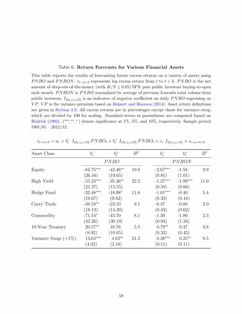
Table 6: Return Forecasts for Various Financial Assets
This table reports the results of forecasting future excess returns on a variety of assets using
PNBO and PNBON . rt→t+3 represents log excess return from t to t+ 3. PNBO is the net
amount of deep-out-of-the-money (with K/S ≤ 0.85) SPX puts public investors buying-to-open
each month. PNBON is PNBO normalized by average of previous 3-month total volume from
public investors. I{bV P,t<0} is an indicator of negative coefficient on daily PNBO regressing on
V P . V P is the variance premium based on Bekaert and Hoerova (2014). Asset return definitions
are given in Section 3.3. All excess returns are in percentages except those for variance swap,
which are divided by 100 for scaling. Standard errors in parentheses are computed based on
Hodrick (1992). (∗∗∗,∗∗ ,∗ ) denote significance at 1%, 5%, and 10%, respectively. Sample period:
1991/01 – 2012/12.
rt→t+3 = ar + b−r I{bV P,t<0} PNBOt + b+r I{bV P,t≥0} PNBOt + cr I{bV P,t<0} + εt+j→t+k
Asset Class b−r b+r R2 b−r b+
r R2
PNBO PNBON
Equity -84.75∗∗∗ -42.46∗∗ 19.8 -2.67∗∗∗ -1.58 9.9(26.16) (19.65) (0.85) (1.01)
High Yield -55.23∗∗∗ -35.26∗∗ 22.2 -1.37∗∗∗ -1.99∗∗∗ 11.0(21.37) (15.55) (0.50) (0.66)
Hedge Fund -32.48∗∗∗ -18.98∗ 11.6 -1.01∗∗∗ -0.40 5.4(10.67) (9.82) (0.33) (0.44)
Carry Trade -38.34∗∗ -23.10 9.1 -0.47 -0.88 2.0(18.13) (14.20) (0.43) (0.62)
Commodity -71.54∗ -43.70 8.1 -1.30 -1.80 2.3(42.26) (30.19) (0.94) (1.34)
10-Year Treasury 20.57∗∗ 10.76 5.5 0.79∗∗ 0.37 3.8(8.92) (10.65) (0.33) (0.45)
Variance Swap (×1%) 13.64∗∗∗ 4.82∗∗ 21.2 0.38∗∗∗ 0.25∗∗ 9.5(4.02) (2.16) (0.11) (0.11)
58
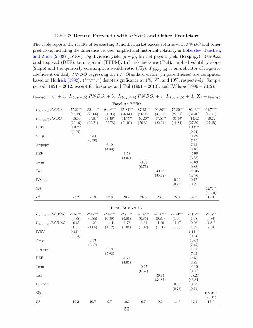
Table 7: Return Forecasts with PNBO and Other Predictors
The table reports the results of forecasting 3-month market excess returns with PNBO and other
predictors, including the difference between implied and historical volatility in Bollerslev, Tauchen,
and Zhou (2009) (IVRV), log dividend yield (d− p), log net payout yield (lcrspnpy), Baa-Aaa
credit spread (DEF), term spread (TERM), tail risk measure (Tail), implied volatility slope
(Slope) and the quarterly consumption-wealth ratio (cay). I{bV P,t<0} is an indicator of negative
coefficient on daily PNBO regressing on V P . Standard errors (in parentheses) are computed
based on Hodrick (1992). (∗∗∗,∗∗ ,∗ ) denote significance at 1%, 5%, and 10%, respectively. Sample
period: 1991 – 2012, except for lcrspnpy and Tail (1991 – 2010), and IVSlope (1996 – 2012).
rt→t+3 = ar + b−r I{bV P,t<0} PNBOt + b+r I{bV P,t≥0} PNBOt + cr I{bV P,t<0} + dr Xt + εt→t+3
Panel A: PNBO
I{bV P,t<0} PNBOt -77.22∗∗∗ -82.44∗∗∗ -94.46∗∗∗ -85.81∗∗∗ -87.33∗∗∗ -90.86∗∗∗ -75.80∗∗∗ -80.13∗∗∗ -62.70∗∗∗
(26.09) (26.66) (30.95) (26.61) (26.96) (31.35) (24.59) (31.40) (22.71)I{bV P,t≥0} PNBOt -18.50 -37.81∗ -47.38∗∗ -44.73∗∗ -46.26∗∗ -47.54∗∗ -36.40∗ -14.42 -59.22
(20.16) (20.21) (22.76) (21.02) (20.32) (22.94) (19.84) (27.59) (37.45)IVRV 0.10∗∗∗ 0.13∗∗∗
(0.04) (0.04)d− p 3.54 11.39
(3.20) (7.75)lcrspnpy 6.19 7.75
(4.89) (8.10)DEF -1.58 -5.96
(3.03) (3.83)Term -0.63 -0.63
(0.71) (0.83)Tail 30.56 -52.06
(35.02) (47.76)IVSlope 0.29 0.17
(0.26) (0.29)cay 92.71∗∗
(46.30)R2 25.2 21.3 22.9 20.4 20.6 20.8 22.4 39.2 19.9
Panel B: PNBON
I{bV P,t<0} PNBONt -2.50∗∗∗ -2.42∗∗∗ -2.47∗∗∗ -2.70∗∗∗ -2.65∗∗∗ -2.56∗∗∗ -2.63∗∗∗ -2.06∗∗∗ -2.07∗∗
(0.85) (0.85) (0.89) (0.86) (0.85) (0.89) (1.00) (1.08) (0.86)I{bV P,t≥0} PNBONt -0.85 -1.20 -1.41 -1.78 -1.61 -1.60 -1.17 0.06 -4.81∗
(1.01) (1.05) (1.12) (1.08) (1.02) (1.11) (1.08) (1.32) (2.60)IVRV 0.13∗∗∗ 0.15∗∗∗
(0.04) (0.04)d− p 3.13 13.63
(3.17) (7.42)lcrspnpy 3.13 1.51
(5.02) (7.92)DEF -1.71 -5.57
(3.03) (3.89)Term -0.27 -0.10
(0.67) (0.85)Tail 26.94 -38.27
(34.87) (46.84)IVSlope 0.36 0.33
(0.28) (0.31)cay 108.03∗∗
(46.11)R2 19.2 10.7 9.7 10.3 9.7 9.7 14.5 32.5 17.7
59

Table 8: PNBO and Measures of Funding Constraints
Panel A reports the results of the OLS regressions of IbV P,t<0 × PNBOt on measures of funding
constraints. Panel B reports the results of return predictability regressions with PNBO and
funding constraint measures. PNBO is the net amount of deep-out-of-the-money (with K/S ≤0.85) SPX puts public investors buying-to-open each month. PNBON is PNBO normalized
by average of previous 3-month total volume from public investors. I{bV P,t<0} is an indicator of
negative coefficient on daily PNBO regressing on V P . V P is the variance premium based on
Bekaert and Hoerova (2014). TED is the TED spread; LIBOR-OIS is the spread between 3-month
LIBOR and overnight indexed swap rates; FG is the funding liquidity measure by Fontaine and
Garcia (2012); ∆lev is the broker-dealer balance sheet growth measure by Adrian, Moench, and
Shin (2010). Standard errors (in parentheses) are computed based on Newey and West (1987)
with 3 lags. (∗∗∗,∗∗ ,∗ ) denote significance at 1%, 5%, and 10%, respectively. Sample period: 1991
– 2012, except for the regressions with LIBOR-OIS (2002 – 2012).
Panel A: IbV P,t<0 × PNBOt = a+ b Xt + et
PNBO PNBON
TED 22.04∗∗ 0.56(10.57) (147.30)
LIBOR-OIS 0.25 -0.17(0.16) (2.04)
FG -4.89∗∗ -200.65∗∗∗
(2.32) (77.30)∆lev 42.59∗∗ 50.86∗∗
(16.68) (23.18)R2 4.3 2.9 1.5 8.9 0.0 0.0 4.4 3.4
Panel B: rt→t+3 = ar + b−r I{bV P,t<0} PNBOt + b+r I{bV P,t≥0} PNBOt + cr IbV P,t<0 + dr Xt + εt→t+3
PNBO PNBON
I{bV P,t<0} PNBOt -79.97∗∗∗ -75.91∗∗∗ -83.52∗∗∗ -53.78∗∗ -2.62∗∗∗ -3.81∗∗∗ -2.57∗∗∗ -1.63∗∗
(24.66) (23.94) (26.65) (22.47) (0.84) (1.23) (0.85) (0.83)I{bV P,t≥0} PNBOt -34.84∗ -38.41∗∗ -42.00∗∗ -37.02 -1.38 -3.07∗∗ -1.50 -3.69
(19.34) (19.37) (19.65) (40.89) (1.02) (1.27) (1.01) (2.79)TED -2.44 -4.83
(3.19) (3.25)LIBOR-OIS -0.05 -0.08
(0.05) (0.05)FG 0.50 0.24
(0.88) (0.86)∆Lev -4.76 -5.82∗
(3.51) (3.41)R2 20.4 34.9 19.6 19.9 14.4 33.1 9.6 18.9
60

Table 9: Return Forecasts with supply shocks
This table reports the results of the return forecasting regressions using supply shocks extracted
using the econometric identification of Rigobon (2003). Normalized supply shocks are formed by
deflating by 3-month trailing average SPX volume. rt+j→t+k represents log market excess return
from month t+ j to t+ k (k > j ≥ 0). Standard errors (in parentheses) are computed based on
Hodrick (1992). (∗∗∗,∗∗ ,∗ ) denote significance at 1%, 5%, and 10%, respectively. Sample period:
1991/01 – 2012/12.
rt+j→t+k = ar + br (supply shock)t + εt+j→t+k
Horizon br σ(br) R2 br σ(br) R2
supply normalized supply
rt→t+1 -12.69∗∗ (4.96) 4.9 -0.48∗∗∗ (0.16) 4.7rt+1→t+2 -10.69∗∗ (4.86) 3.5 -0.37∗∗∗ (0.14) 2.7rt+2→t+3 -15.07∗∗∗ (4.58) 7.0 -0.23∗ (0.13) 1.0rt+3→t+4 -11.71∗∗ (4.75) 4.2 -0.14 (0.13) 0.4rt→t+3 -38.03∗∗∗ (11.76) 13.6 -1.06∗∗∗ (0.32) 7.0
61

Table 10: Return Forecasting Outside the Financial Crisis
This table reports the results of the return forecasting regressions in pre- and post-crisis
subsamples. rt→t+3 indicate market excess return one- and three- month ahead, respectively.
PNBO is the net amount of deep-out-of-the-money (with K/S ≤ 0.85) SPX puts public
investors buying-to-open each month. PNBON is PNBO normalized by average of previous
3-month total volume from public investors. I{bV P,t<0} is an indicator of negative coefficient on
daily PNBO regressing on V P . V P is the variance premium based on Bekaert and Hoerova
(2014). Standard errors (in parentheses) are computed based on Hodrick (1992). (∗∗∗,∗∗ ,∗ )
denote significance at 1%, 5%, and 10%, respectively. Pre-crisis: 1991/01 - 2007/11. Post-crisis:
2009/06 - 2012/12.
rt→t+3 = ar + b−r I{bV P,t<0} PNBOt + b+r I{bV P,t≥0} PNBOt + cr I{bV P,t<0} + εt+j→t+k
b−r b+r R2 b−r b+
r R2
PNBO PNBON
Pre-crisis -66.50∗∗ 21.91 3.8 -1.85∗∗ -0.12 5.3(27.53) (22.90) (0.92) (1.12)
Post-crisis -50.88∗∗ -15.73 17.4 -4.87∗∗ -1.02 19.6(25.72) (33.42) (2.39) (3.61)
62

Table 11: Return Forecasts with PNOI
This table reports the results of the return forecasting regressions using PNOI and PNOIN .
rt+j→t+k represents log market excess return from t + j to t + k (k > j ≥ 0). PNOI is the
end-of-month public net open interest for deep-out-of-the-money (K/S ≤ 0.85) puts. PNOIN
is PNOI normalized by the sum of public long and short open interest. V P is the variance
premium based on Bekaert and Hoerova (2014). I{bV P,t<0} is an indicator of negative coefficient
on daily PNBO regressing on V P . Standard errors (in parentheses) are computed based on
Hodrick (1992). (∗∗∗,∗∗ ,∗ ) denote significance at 1%, 5%, and 10%, respectively. Sample period:
1991/01 – 2012/12.
rt+j→t+k = ar + b−r I{bV P,t<0} PNOIt + b+r I{bV P,t≥0} PNOIt + crI{bV P,t<0} + εt+j→t+k
Horizon b−r b+r R2 b−r b+
r R2
PNOI PNOIN
rt→t+1 -25.10∗∗∗ -11.72 8.1 -3.71∗∗∗ -1.23 5.6(8.65) (7.93) (1.11) (1.17)
rt+1→t+2 -19.79∗∗ -1.65 5.3 -2.11∗ -0.25 2.7(9.59) (4.72) (1.17) (0.99)
rt+2→t+3 -19.34∗∗ -4.67 4.5 -2.21∗∗ -0.26 2.0(7.73) (7.66) (0.97) (1.19)
rt+3→t+4 -9.75 -17.17∗ 4.2 -1.32 -2.32∗ 2.4(6.85) (9.18) (0.96) (1.29)
rt→t+3 -64.22∗∗∗ -18.05 14.7 -8.03∗∗∗ -1.74 7.8(23.47) (13.50) (2.68) (2.28)
63

Table 12: Comparison with GPP Table 2
This table replicates results in Garleanu, Pedersen, and Poteshman (2009). The table reports
regression coefficients from regressing option expensiveness, measured by the average implied
volatility of ATM options minus a reference model-implied volatility used in Bates (2006), on
measures of option demand. NetDemand and JumpRisk are the equal- and vega-weighted public
net open interest (or net volume) for all SPX options. t-stats are computed based on Newey and
West (1987) standard errors with 10 lags. (∗∗∗,∗∗ ,∗ ) denote significance at 1%, 5%, and 10%,
respectively.
Net Open Interest Net Volume
Replicated Results GPP ResultsNetDemand JumpRisk NetDemand JumpRisk NetDemand JumpRisk
1996/01-1996/10 2.1×10⁻⁷ 4.5×10⁻⁶ 2.1×10⁻⁷ 6.4×10⁻⁶ 1.6×10⁻⁸ -5.1×10⁻⁶
t-stat (0.72) (0.49) (0.87) (0.79) (0.10) (-0.23)
1997/10-2001/12 3.8×10⁻⁷∗∗ 2.6×10⁻⁵∗∗∗ 3.8×10⁻⁷ 3.2×10⁻⁵∗∗∗ 4.7×10⁻⁶∗∗ 4.9×10⁻⁵∗∗
t-stat (2.17) (2.80) (1.55) (3.68) (2.25) (2.57)
2002/01-2012/12 -9.9×10⁻⁸∗∗∗ -7.8×10⁻⁶∗∗ -6.7×10⁻⁷∗∗ -5.2×10⁻⁵∗∗∗
t-stat (-3.13) (-2.40) (-2.35) (-3.32)
64

Table A1: Model Parameters
risk aversion: γ 4time preference: δ 0.03mean growth of endowment: g 0.025volatility of endowment growth: σc 0.02mean intensity of disaster: λ 1.7%speed of mean reversion for disaster intensity: κ 0.142disaster intensity volatility parameter: σ 0.05dealer risk aversion parameter: α 1.0
65

Table A2: Comparing SPX vs. SPY Trades
This table reports the results of the return forecasting regressions based on two measures of public
net buying-to-open volume: public net buying to open for SPX options (PNBOSPX , denoted
elsewhere as simply PNBO) and public net buying to open for SPY options (PNBOSPY ).
PNBONSPX and PNBONSPY are PNBOSPX and PNBOSPY normalized by average of
previous three month total volume of all options. I{bV P,t<0} is an indicator of negative coefficient
on daily PNBO regressing on V P . All options in computing PNBO are DOTM, as defined by
K/S ≤ 0.85. Standard errors (σ) in parentheses are computed based on Hodrick (1992). (∗∗∗,∗∗ ,∗ )
denote significance at 1%, 5%, and 10%, respectively. Sample period: 2005/05 – 2012/12.
A: V Pt = aV P + bV P PNBOt + cV P Jt × PNBOt + dV P Jt + εvtB: rt+j→t+k = ar + b−r I{bV P,t<0} PNBOt + b+r I{bV P,t≥0} PNBOt + crI{bV P,t<0} + εt→t+3
Panel A
bV P cV P R2 bV P cV P R2
PNBOSPX PNBOSPY
V P 18.41 -7.09∗∗∗ 35.5 29.13 5.20 23.4(35.51) (2.31) (80.82) (4.82)
PNBONSPX PNBONSPY
V P 2.60 -0.77∗∗∗ 36.7 -92.61 25.12 23.2(2.94) (0.20) (245.43) (50.04)
Panel B
Return b−r b+r R2 b−r b+
r R2
PNBOSPX PNBOSPY
rt→t+1 -19.10∗∗∗ -30.85∗∗∗ 18.0 -8.46 11.39 2.4(8.70) (12.99) (15.22) (9.34)
rt→t+3 -84.07∗∗∗ -45.16∗∗∗ 39.4 -20.95 15.00 3.8(25.41) (21.42) (29.43) (15.79)
PNBONSPX PNBONSPY
rt→t+1 -1.55∗∗∗ -2.48∗∗∗ 15.0 -130.46 119.74 3.2(0.68) (1.05) (137.04) (101.04)
rt→t+3 -7.04∗∗∗ -3.64∗∗∗ 35.3 -370.76 117.24 5.4(2.07) (1.71) (279.40) (166.30)
66

Table A3: Indicators of Supply Environment
This table reports the indicators of supply environment based on the sign of bV P,t and based on
the Cohen, Diether, and Malloy (2007) (CDM) method. The months listed include those
associated with major events in the global financial markets. They also include the pe-
riod of 2007/11 to 2009/06, the period of the 2008 financial crisis. For more details of the
events during the 2008 financial crisis, see the Federal Reserve Bank of St. Louis webpage
(https://www.stlouisfed.org/financial-crisis/full-timeline).
Month IbV P,t<0 CDM Events
1997/10 0 0 Asian financial crisis1998/11 1 0 Russian financial crisis2003/04 1 0 Start of the Iraq War2007/08 0 1 Quant crisis
2007/11 1 1 Liquidity deterioration in interbank funding market2007/12 1 0 Creation of TAF2008/01 1 0 Bank of America acquisition of Countrywide2008/02 0 0 Northern Rock taken into state ownership2008/03 0 1 Sale of Bear Sterns to JPMorgan2008/04 1 1 FOMC rate cut2008/05 0 1 FOMC expands the list of eligible collateral for TSLF2008/06 1 0 S&P downgrade of AMBAC and MBIA2008/07 1 1 Failure of IndyMac2008/08 1 1 FOMC maintains federal funds rate target2008/09 1 1 Lehman Bankruptcy2008/10 0 0 Establishment of TARP2008/11 1 0 Creation of TALF2008/12 1 1 Fed extension of liquidity facility2009/01 0 1 Treasury, Fed, FDIC assistance to BofA2009/02 1 1 Increase of TALF to $1 trillion2009/03 0 12009/04 0 02009/05 1 12009/06 0 0 Large banks’ repayments of bailout funds
2009/12 1 0 Escalation of Greek debt crisis2010/04 0 0 Greece seeks financial support2010/05 1 0 Establishment of EFSM and EFSF2010/09 1 1 Second Greek bailout installment2011/06 1 0 Merkel agrees to Greece bondholder role2011/10 1 0 Call for a Greek referendum
67