Proc. Schl. ITE Tokai Univ. Vol. ,No. ,2010,pp. -

Vol. XXXI, 2009

―1―

*1 Graduate student, Department of management systemsengineering

*2 Professor, Department of management systems engineering

Demand and Price Forecasting Models for Strategic and Planning

Decisions in a Supply Chain

by

Vichuda WATTANARAT*1, Phounsakda PHIMPHAVONG*1 and Masanobu MATSUMARU*2

(Received on October 30, 2010 and Accepted on January 25, 2011)

Abstract Procurement and sales forecasting are a fundamental approach to the estimation of inventory. The accuracy is an

essential factor for a firm on cost of manufacturing. Forecasting is an important for all strategic and planning decisions in a supply chain. Forecasts of product demand, materials, labor, financing are useful inputs to scheduling, acquiring resources, and determining resource requirement. However, highly volatile and correlated demand caused inaccuracy. This paper aims to compare real option method and ARIMA model method to be able to predict a precise future procurement and sales. To validate the forecasting model, we use the real world data which are demand obtained from one die casting company and copper price. The result shows that real option model is outperforming ARIMA model quite significantly in case the data has high volatility.

Keywords: Forecast, Volatile, Demand, Geometric Brownian motion, ARIMA methodology

1. Introduction

Smoothing the demand and supply is the main problem in supply chain management. Under supply leads to the loss of potential revenue, over supply incurs extra carrying cost of the excess product. Procurement and inventory control are of active area of research to gain the competitiveness for the company. The optimal quantity can enable the company to achieve the cost reduction. To obtain the optimality in supply chain, we have to deal with making the decision about the future event, produce to secure the future sale. This involves with forecasting the unforeseen data for example demand and price. The less deviation from the real value the less risk we have from doing the operation. Demand forecasting plays a very crucial role in production planning of the manufacturing. It is the main input for the capacity planning which links to various chain of supply including inventory, logistic and service level. Demand and price is usually difficult to forecast due to their uncertainty nature. Basically demand should show an increasing trend over the long term period. When we look at the short term period, we often see the unexpected move either going up or down. If we include more realistic possibility of the economic factor to try to understand and

predict movement of the demand, we can clearly see from the history that will not always suppose to have an upward trend even in the long term demand. This case is clearly noticed in the time of economic crisis. Besides, competition and advancement of technology also erode the demand of one company to another. Taking the example of mobile music industry like Sony that loses the market share to Apple product. In this paper we compare the new forecasting method that is apply to the forecast of demand and price. There are many ways that we can adopt for forecasting for example linear regression, moving average, ARMA, ARIMA. Here we compare the real option approach with the ARIMA model and conclude what kind of data is best suited for these kind of forecasting. Real option approach is originated from the finance study. It is used to value the value of uncertainty in an investment. Real option is different from traditional investment criteria like Net Present Value (NPV) in that unexercised choices have also future value and should contribute the evaluation.

2. Literature review

Real option approaches which is based on the diffusion process of the variable for doing the forecast is quite a new field of study. The most common diffusion process that is used in real option study is Geometric Brownian Motion

－ 36－ － 37－

東海大学紀要情報通信学部vol.3,No2,2010,pp.37-42

Paper

Times, Times and Times

Proc. Sch. ITE Tokai University

―2―

(GBM). GBM is used to replicate the movement or character of the object of study in many fields of study e.g. particle movement in physic, the price of the underlying asset in the financial study, water level in reservoir etc. Huang [1] applies real option in forecasting the demand of products that has correlated to one another and that have high volatility. The kind of product that has such kind of nature is referred to IT product. In their research they forecast the demands of 4 products that relate to one another. If one product changes, the volume of other products also changes. The GBM model is used to replicate the future demand in capacity studies [2]. They studied capacity utilization over time assuming that demand followed a GBM. Yon [3] also studied about the capacity planning. They analyzed in case of demand has high volatility and machine and process technology are advanced at a rapid pace, making it difficult to do the capacity planning in the semiconductor industry. They assume the demand to follow the GMB. They simulate and compare the result of the profit in two difference scenarios. Real option by mean of GBM has also been used extensively in making investment decision as in Dixit and Pindyck [4]. It can be used to find the optimal time to invest, evaluate option to postpone investment, option to shut down the business, option to expand business etc. in which the traditional investment criteria cannot handle with well. An autoregressive integrated moving average (ARIMA) is one of well known model in statatistic and econometrics. It is used to study the behavior of time series and predict the future out of the time series. The simple way to think about the ARIMA model is that it is the combination of random walk and trend model. This characteristic is very similar to the GBM and it is a good candidate for the comparison.

For a high volatile demand product, Makridakis and Wheelwright [5] extended the time series analysis by including moving average, regression, exponential smoothing, and seasonal exponential smoothing. The ARIMA methodology is developed by Box and Jenkins [6]. It is a mathematical model for forecasting a time series by fitting it with the data and using the fitted model for forecasting. R.J. Hyndman [7], Pankratz [8] and Martin, R.D., Samarov, A. and W. Vandaele [9] study ARIMA model in application. Metcalf & Hasset [10] study the mean reversion format equation, and it has more economic logic than the geometric Brownian model. Carlos and David [11] explore the main stochastic price processes used to model energy spot and forward prices for derivatives valuation and risk management. They apply a Geometric Brownian motion to be a random walk with mean reversion. In our research we compare the forecasting methods which are real option method, ARIMA

model for the estimation of procurement and sales. We compare our study with the previous study in Table 1.

Table 1 Previous study comparison

Previous Study Details

Makridakis and Wheelwright (1985)

Time series analysis by including moving average, regression, exponential smoothing, and seasonal exponential smoothing

Ming-Guan Huang (2008) Real option approach-based demand forecasting method for a range of products with highly volatile and correlated demand

James D. Hamilton ( Book,1994)

Analyze vector auto regressions, generalized method of moments, the economic and statistical consequences of unit roots, time-varying variances, and nonlinear time series models

The outline of this study is as follow: In section 2 we explain the methodologies and how to estimate the future value. We set a numerical simulation and illustrate results in section 3. We prefer to use MATLAB to simulate the simulation of real option method, Eviews for ARIMA model. Finally, we conclude a summary of our findings.

3. Forecasting Methodology 3.1 Geometric Brownian motion Geometric Brownian motion is originated in physics as a diffusion process used to describe the partial motion when it falls. Let Xt be the value of the data at time t and assume it to follow the Geometric Brownian Motion, we have the diffusion specify in equation (1). In this equation there are two parts. The first part on the right hand side is the mean growth of the diffusion and the second part on the right hand side of the equation is the volatility.

tttt dzXdtXdX σμ += (1)

Where dtdz tt ε= is the standard increment of Wiener process or the white noise, μ and σ are drift and variance terms respectively. zt has the following 2 properties: Property 1: The change in the value of z, dz, over a time internal of length Δt is proportional to the square root of Δt

Demand and Price Forecasting Models for Strategic and Planning Decisions in a Supply Chain

－ 38－ － 39－

Times Times Times Times Times

Vol. XXXI, 2009

―3―

where the multiplier is random. In specific dz=z(t+ Δt)-z(t)=εΔt, where ε is a standard normal random variable. Hence values of dz follow a normal distribution with mean 0 and variance equal to the change in time (Δt) over which dz is measured. Property 2: The changes in the value of zt for any non-overlapping intervals of time are independent. Let f=ln Xt and expand f according to the Taylor series we have

......)(21)( 2

2

2++= t

tt

tdX

dXfddX

dXdfdf (2)

Then apply Ito lemma to (2), we have that Δt that has power greater than 2 will approach to zeros quicker when Δt is small. We have

22

2)(

21)( t

tt

tdX

dXfddX

dXdfdf += (3)

Substitute (1) into (3) and rearrange we have

ttXX tt Δ+Δ⎟⎠⎞

⎜⎝⎛ −=−+ σεσμ 2

1 21lnln (4)

⎥⎦

⎤⎢⎣

⎡Δ+Δ⎟

⎠⎞

⎜⎝⎛ −=+ ttXX tt σεσμ 2

1 21exp (5)

Equation (5) is the discrete version of Geometric Brownian Motion that we will use to simulate the forecast of demand and price in this study. 3.2 Calibrate the parameter The Geometric Brownian Motion process can formally be defined as Xt ,0≤ t ≤∞, the random variable of Xt/Xt+1 is independent of all values of the variable up to the time t and if in addition ln(Xt/Xt+1) has a normal distribution with mean μt and variance σ2t. Let rt be the difference between logarithm Xt and Xt-1 we have

tt

t rXX

=⎟⎟⎠

⎞⎜⎜⎝

⎛

−1ln (6)

In finance, (6) represent the logarithm of the return which is necessary assumption because the value of the underlying asset that is assumed to follow Geometric Brownian Motion should have a value greater or equal to zero. rt also implies the growth rate of the observed data in each period. In order to estimate the parameter to use in the forecast model as specified by equation (5) we following equations

trE t Δ−= )2()( 2σμ (7)

trV r Δ= 2)( σ (8)

n

r

r

n

tt∑

== 1 (9)

∑=

−−

=n

ttr rr

ns

1

)()1(

1 (10)

t

sr

Δ=σ (11)

t

st

rt

r r

Δ+

Δ=+

Δ=

22ˆ 22σμ (12)

3.3 ARIMA Model In supply chain management, An autoregressive integrated moving average has been used to in many problems ranging from finding optimal order policy, predicting customer demand, predicting the price movement, inventory management etc. The autoregressive moving average (ARMA) model was introduced by Box and Jenkins (1976). It consists of two parts, an autoregressive (AR) part and a moving average (MA) part. Specifically, the three types of parameters in the model are: the autoregressive parameters (p), the number of differencing passes (d), and moving average parameters (q). Models are summarized as ARIMA (p, d, q). ARIMA combines auto regression-which fits the current data point to a linear function of some prior data points and moving averages adding together several consecutive data points and getting their mean, and then using that to compute estimations of the next value. With enough elements regressed and averaged, we can fit an approximation too many time series and with low discrepancy. We find the best ARIMA (p,d,q) model condition by comparing the Akaike information criterion (AIC). The smallest AIC is the most suitable condition. An ARIMA (p,d,q) model contains three different kinds of parameters: (1) the p AR-parameters; (2) the q MA-parameters the number of lagged forecast errors in the prediction equation. (3) d the number of differences. This amounts to a total of (p,d,q) parameters to be estimated. These parameters are always estimated on using the stationary time series which is stationary with respect to its variance and mean. To identify the appropriate ARIMA model for a time series, we have to identifying the order(s) of differencing needing to stationary the series and remove the gross features of seasonality, perhaps in conjunction with a variance-stabilizing transformation such as logging or

－ 38－

Vichuda WATTANARAT・Phounsakda PHIMPHAVONG・Masanobu MATSUMARU

－ 39－

Times, Times and Times

Proc. Sch. ITE Tokai University

―4―

deflating. An notation AR(p) refers to the autoregressive model of order p. An AR(p) model is defined as (13)

where are the parameters of the model, c is a constant and tε is white noise. An MA model is a common approach for modeling univariate time series models. (14) where μ is the mean of the series, the θ1, ..., θq are the parameters of the model and the εt, εt−1,... are white noise error terms. The value of q is called the order of the MA model. An ARMA consists of two parts, an autoregressive (AR) part and a moving average (MA) part. The model is usually then referred to as the ARMA(p,q) model where p is the order of the autoregressive part and q is the order of the moving average part.

(15)

An ARIMA model is a generalization of an ARMA model. The model is generally referred to as an ARIMA(p,d,q) model where p, d, and q are non-negative integers that refer to the order of the autoregressive, integrated, and moving average parts of the model.

4. Empirical analysis

Decisions make in advance of uncertain events. And forecasting is an important for all strategic and planning decisions in a supply chain. Especially, forecasts of product demand, materials are important inputs to scheduling, acquiring resources, and determining resource requirement.

We use the data of the medium and small-sized business in real world and check the effectiveness of a suggested model. This company accepts an order from the upstream company. Because there is a change in this order, this company must have many stocks to avoid lack. As a result, this company must risk a burden for a cost to maintain a stock. Therefore, it is important that the company predicts quantity of order from the upstream company. If we predict the volume precisely, this company reduces the inventory cost. The reduction of the inventory cost in the model that we suggested had a big influence on the improvement of corporate earnings.

4.1 Data It assumes that the forces which influenced past value will continue to exist in the future. In this section, we follow the forecast methodology to calculate the numerical value of demand and price. We follow the forecast methodology to calculate the numerical value of demand and price. For the

numerical experiment, we use 122 weeks of data (from November, 2004 to December, 2008) for estimation by using Geometric Brownian motion, ARIMA model and mean Reversion. 4.2 Empirical results of Geometric Brownian motion In this research, we apply to both forecasting models to the forecast the demand of one die casting company and the price of copper. We use the data from November 2004 to December 2008. The actual demand shows the seasonality in the data series. For the actual price of copper, the data set shows high volatility and covers the period of the financial crisis. (1)Results of demand For the illustrative purpose, we simulate demand 1000 rounds for each period by using MATLAB. Figure 1 is a result from real option method. Real option method provides the forecasting value along with actual value as well. This method can capture demand changes quite accurately.

All the data were acquired on statistical software for economic analysis, called EViews, which is developed by Quantitative Micro Software (QMS). We analyze demand and price data which are separated to be 122 numbers of data. We follow the parameter setting from November 2004 to December 2008.

Total Deamnd forecast

0

20000

40000

60000

80000

100000

120000

140000

1 12 23 34 45 56 67 78 89 100 111 122 133 144 155 166 177 188 199 210

Time (Week)

Dem

and

(kg)

Total Demand

Total Demand Forecast

Figure 1 Demand forecast

(2)Results of price We try to find the simulation result of mean reversion in price with 1000 times estimation.

Figure 2 Price forecast

Actual Price

0

200

400

600

800

1000

1 12 23 34 45 56 67 78 89 100 111 122 133 144 155 166 177 188 199 210

Time (Week)

Price (

Yen)

Actual Price Forecasting Price

tptpttt XXXcX εφφφ +++++= −−− ...2211 1

pφφφ ,,, 21 LL

qtqtttx −− ++++= εθεθεμ L11

tqtqt

ptptt XXcX

εεφεφ

φφ

++++

+++=

−−

−−

...

...

11

11

Demand and Price Forecasting Models for Strategic and Planning Decisions in a Supply Chain

－ 40－ － 41－

Times Times Times Times Times

Vol. XXXI, 2009

―5―

4.3 Empirical results of ARIMA model 4.3.1 Numerical experiment of Demand following real option method We demonstrate a result of AIC in Table 2 with the different value of d in ARIMA (p,d,q) model. The best ARIMA (p,d,q) parameters for ARIMA model for demand is computed as ARIMA (9,1,9) that AIC is 22.4. We assume to use ARIMA (9,1,9) which offers the best Akaike information criterion for our simulation.

We demonstrate our forecasting result by using ARIMA (9,1,9) in Figure 3 as below. In the beginning ARMA model can produce demand forecast quite well but in the long run the forecast accuracy is getting lower.

Table 2 ARIMA parameter for total demand

1.1.X 2.1.X 3.1.X 4.1.X 5.1.X 6.1.X 7.1X 8.1.X 9.1.X 10.1.X

X.1.1 22.53 22.54 22.55 22.44 22.52 22.52 22.55 22.54 22.55 22.55

X.1.2 22.52 22.46 22.55 22.45 22.52 22.49 22.56 22.55 22.51 22.54

X.1.3 22.53 22.53 22.56 22.54 22.53 22.49 22.48 22.49 22.51 22.52

X.1.4 22.55 22.51 22.42 22.44 22.43 22.47 22.46 22.51 22.51 22.51

X.1.5 22.54 22.52 22.43 22.45 22.42 22.41 22.4 22.41 22.44 22.41

X.1.6 22.51 22.52 22.44 22.41 22.43 22.4 22.38 22.43 22.52 22.41

X.1.7 22.52 22.5 22.46 22.41 22.41 22.44 22.44 22.46 22.53 22.46

X.1.8 22.53 22.52 22.46 22.41 22.46 22.42 22.48 22.46 22.42 22.43

X.1.9 22.54 22.52 22.45 22.42 22.43 22.43 22.43 22.45 22.4 22.4

X.1.10 22.52 22.5 22.52 22.43 22.49 22.5 22.48 22.51 22.43 22.41

Total Demand Forecast (ARIMA Model)

0

20000

40000

60000

80000

100000

120000

1 13 25 37 49 61 73 85 97 109 121 133 145 157 169 181 193 205

Time (Week)

Dem

and

(Kg)

Actual Demand

Forecast Demand

Figure 3 Price forecast (ARIMA (9,1,9)) The first step to simulate the forecasting price by using ARIMA model is to find the best AIC as shown in Table 3. We use ARIMA (6,1,3) model which provides the best AIC, 8.72. The 1000 round simulation result is shown in Figure 4. We can use ARIMA model to forecast the low volatility price accurately through all period. 4.3.2 Comparison of demand forecasting When we compare the result of forecasting between real option method and ARIMA model, we see that both method give quite similar degree of accuracy.

Table 3 ARIMA parameter for total price 1.1.X 2.1.X 3.1.X 4.1.X 51.X 6.1.X 7.1X 8.1.X 9.1.X 10.1.X

X.1.1 8.902 8.898 8.898 8.911 8.926 8.939 8.9503 8.9581 8.970 8.980

X.1.2 8.892 8.901 8.907 8.921 8.934 8.904 8.9572 8.9713 8.943 8.973

X.1.3 8.897 8.904 8.916 8.93 8.907 8.72 8.9324 8.9479 8.949 8.955

X.1.4 8.9 8.913 8.922 8.936 8.912 8.917 8.8992 8.9239 8.906 8.937

X.1.5 8.908 8.919 8.931 8.91 8.913 8.747 8.7236 8.925 8.927 8.943

X.1.6 8.918 8.928 8.939 8.904 8.919 8.94 8.9138 8.9272 8.948 8.941

X.1.7 8.928 8.938 8.912 8.891 8.938 8.933 8.8775 8.9365 8.96 8.95

X.1.8 8.938 8.903 8.92 8.92 8.929 8.927 8.932 8.9493 8.9462 8.91656

X.1.9 8.927 8.918 8.924 8.919 8.919 8.911 8.9324 8.9511 8.9506 8.93665

X.1.10 8.926 8.938 8.93 8.906 8.922 8.935 8.9436 8.8277 8.9519 8.94281

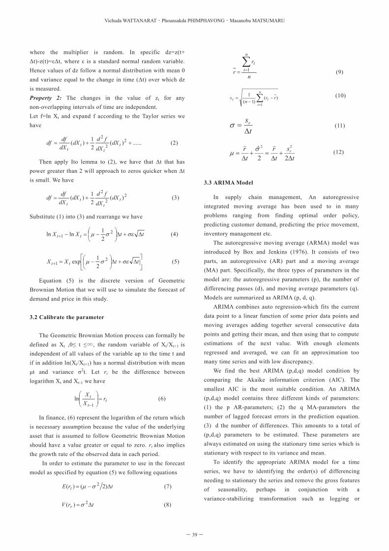
However real option approaches does a slightly better

performance than ARIMA model. Demand data does not show high degree of fluctuation. This is an important condition that is contributed to the level of accuracy of in each method. To verify the precision of forecasting model, we compare the actual and forecast result again. From Figure 4 and Figure 5, the real option method presents the best forecast accuracy.

Total Demand Forecast

0

20000

40000

60000

80000

100000

120000

140000

1 13 25 37 49 61 73 85 97 109 121 133 145 157 169 181 193 205

Time (Week)

De

man

d (K

g)

Actual Demand Real Option

ARIMA Mean Reversion

Figure 4 Demand forecasting result

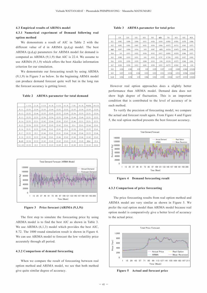
4.3.3 Comparison of price forecasting

The price forecasting results from real option method and ARIMA model are very similar as shown in Figure 5. We prefer the real option model than ARIMA model because real option model is comparatively give a better level of accuracy to the actual price.

Total Price Forecast

0

200

400

600

800

1,000

1 15 29 43 57 71 85 99 113 127 141 155 169 183 197 211

Time (Week)

Price (

Yen)

Actual Price Real Option

ARIMA Mean Reversion

Figure 5 Actual and forecast price

－ 40－

Vichuda WATTANARAT・Phounsakda PHIMPHAVONG・Masanobu MATSUMARU

－ 41－

Times, Times and Times

Proc. Sch. ITE Tokai University

―6―

This can be explained by the name of the change in price data. The price data has a higher level of volatility comparing the level of volatility of demand. This explains why Real options approach outperforms ARIMA. In short, we can say that in case of high volatility data Real options approach is preferred over ARIMA.

We show the comparison of the absolute deviation of demand and price in table 4 and table 5.

Table 4 Absolute deviation of demand

Real Option% AD

ARIMA Model%AD

0.182

0.168

Table 5 Absolute deviation of price

Real Option% AD ARIMA Model%AD

0.06 0.6

5. Conclusion

In this study we compare the forecasting methods that are

used to forecast demand and price. We use real option approach forecasting method that is based on Geometric Brownian motion for the prediction. This model is good in capturing the trend and the volatility of the data, which are the common characteristic of many data type especially in finance and supply chain management. The model is used to predict in a short term period. We highlight and compare the result with ARIMA method that is one of the famous models used to forecast time series. The result shows that real options approach perform better in both sets of data that we used to test. Especially when the data has a high volatility, real options shows less deviation than ARIMA model. Besides that the time interval and availability of data set also have a crucial impact on the accuracy of the forecast. Deseasonality of data and data segmentation would probably improve the performance of the forecast and still remain an interest of our future research.

Reference

[1] Ming-Guan Huang (2008), Real options approach-based demand forecasting method for a range of profits with highly volatile and correlated demand, European journal of operational research [2] Yon-Chun Chou, C.-T Cheng, Feng-Cheng Yang, Yi-Yu Liang, Evaluation alternative capacity strategies in semiconductor manufacturing under uncertain demand and price scenarios", International journal of production

economics, 2006. [3] Carlos and David, “Mean Reverting Processes-Energy Price Processes Used For Derivatives Pricing & Risk Management”, Commodities Now, June 2001. [4] Dixit and Pindyck, Investment under uncertainly,1994 [5] Makridakis,S.,Wheelwright,S.C.,1995, Forecasting methods for Management, John Wiley & Sons, New York [6] Box George and Jenkins Gwilym (1970), Time series analysis: Forecasting and control, San Francisco, Holden- Day. [7] Makridikis, S., S.C. Wheelwright, and R.J. Hyndman (1998), Forecasting: methods and applications, New York, John Wiley & Sons [8] Pankratz, A. (1983), Forecasting with univariate Box–Jenkins models: concepts and cases, New York, John Wiley & Sons [9] Martin, R.D., Samarov, A. and W. Vandaele, "Robust Methods for ARIMA Models", In Time Series Analysis: Theory and Practice 1, Proceedings of the International Conference held at Valencia, Spain, June 1981, Anderson, O. D. (Ed.) (1982), Amsterdam: North-Holland Publishing Company, pp.755-756. [10] Metcalf & Hasset (1995), "Investment under Alternative Return Assumptions Comparing Random Walks and Mean Reversion", Journal of Economic Dynamics and Control, vol.19, November 1995, pp.1471-1488 [11] Whitt, W., “The stationary Distribution of a Stochastic Clearing Process,” Operations Research 29(2), pp.249-308 (1981)

Demand and Price Forecasting Models for Strategic and Planning Decisions in a Supply Chain

－ 42－ － 43－