
Deliverable2.3 Draft v0 5.2
68
Case Studies for testing the digitisation process 1| Page DELIVERABLE Project Acronym: 3D-ICONS Grant Agreement number: 297194 Project Title: 3D Digitisation of Icons of European Architectural and Archaeological Heritage Case Studies for Testing the Digitisation Process Interim report Revision: interim 0.5.2 Authors: Anestis Koutsoudis, CETI; Blaz Vidmar, CETI; Fotis Arnaoutoglou, CETI; Fabio Remondino, FBK; Contributors: Sheena Bassett, MDR Partners; Christos Chamzas, CETI; Project co-funded by the European Commission within the ICT Policy Support Programme Dissemination Level P Public X C Confidential, only for members of the consortium and the Commission Services
Transcript of Deliverable2.3 Draft v0 5.2

Case Studies for testing the digitisation process 1| P a g e
DELIVERABLE
Project Acronym: 3D-ICONS
Grant Agreement number: 297194
Project Title: 3D Digitisation of Icons of European Architectural and Archaeological Heritage
Case Studies for Testing the Digitisation Process
Interim report
Revision: interim 0.5.2
Authors: Anestis Koutsoudis, CETI; Blaz Vidmar, CETI; Fotis Arnaoutoglou, CETI; Fabio Remondino, FBK; Contributors: Sheena Bassett, MDR Partners; Christos Chamzas, CETI;
Project co-funded by the European Commission within the ICT Policy Support Programme Dissemination Level
P Public X C Confidential, only for members of the consortium and the Commission Services
Case Studies for testing the digitisation process 2| P a g e
Revision History
Revision Date Author Organisation Description 0.2 1/12/12 A. Koutsoudis,
B. Vidmar, F. Arnaoutoglou
CETI Initial draft document discussion
0.4 7/1/13 A. Koutsoudis, B. Vidmar, F. Arnaoutoglou, F. Remondino
CETI, FBK Draft integrating feedback from F. Remondino, Sheena Bassett, Christos Chamzas
0.5 5/3/13 A. Koutsoudis, F. Remondino
CETI, FBK Draft integrating case 4, from F. Remondino,
0.5.1 5/3/13 A. Koutsoudis, F. Remondino
CETI, FBK Draft integrating case 2, from F. Remondino,
0.5.2 21/3/13 A.Koutsoudis, F. Remondino
CETI,FBK Relocate, extend and update content based on partners comments, renumber figures and tables
Statement of originality: This deliverable contains original unpublished work except where clearly indicated otherwise. Acknowledgement of previously published material and of the work of others has been made through appropriate citation, quotation or both.

Case Studies for testing the digitisation process 3| P a g e
Contents
Revision History 2
1 EXECUTIVE SUMMARY 5
2 3D DIGITISATION METHODOLOGIES 6
3 SELECTING AN APPROPRIATE 3D ACQUISITION METHODOLOGY 10
4 3D DATA POST-PROCESSING 12 4.1 An Overview 12 4.2 On 3D point cloud processing 13 4.3 On 3D mesh processing 13 4.4 An overview of some popular 3D file formats 14
5 3D DIGITISATION CASE STUDIES 17
5.1 Case Study 1 – The Kioutouklou Baba Bekctashic Tekke 18 Possible 3D Digitisation Solutions ............................................................................................. 18 5.1.1 Purpose behind the specific case study ...................................................................................... 18 5.1.2 Collecting Data ........................................................................................................................... 18 5.1.3 3D Model Generation based on SFM-DMVR ........................................................................... 20 5.1.4 Different Methodologies Data Comparison and Results Evaluation ......................................... 22 5.1.5 3D Data Post Processing ............................................................................................................ 24 5.1.6 Metadata Creation ...................................................................................................................... 25 5.1.7 3D Data Formats for Publication ................................................................................................ 25 5.1.8 Conclusions ................................................................................................................................ 26 5.1.9
5.2 Case Study 2 – Etruscan tomb 28 The heritage and the selected 3D recording technique ............................................................... 28 5.2.1 3D surveying and modelling ...................................................................................................... 29 5.2.2 Metadata Creation ...................................................................................................................... 32 5.2.3 3D Data Formats for Publication ................................................................................................ 32 5.2.4
5.3 Case Study 3 -‐ A marble fragment 33 The heritage and the selected 3D recording technique ............................................................... 33 5.3.1 3D surveying and modelling ...................................................................................................... 33 5.3.2 Metadata Creation ...................................................................................................................... 35 5.3.3 3D Data Formats for Publication ................................................................................................ 35 5.3.4
5.4 A funerary ash urn 36 The heritage and the selected 3D recording technique ............................................................... 36 5.4.1 3D surveying and modelling ...................................................................................................... 36 5.4.2 Metadata Creation ...................................................................................................................... 37 5.4.3 3D Data Formats for Publication ................................................................................................ 37 5.4.4
5.5 Case Study 5 – A Cycladic Female Figurine 38 Possible 3D Digitisation Solutions ............................................................................................. 39 5.5.1 Purpose behind the specific case study ...................................................................................... 39 5.5.2 Collecting data ............................................................................................................................ 40 5.5.3

Case Studies for testing the digitisation process 4| P a g e
3D Model Generation based on SFM-DMVR ........................................................................... 42 5.5.4 Data Comparison and Results Evaluation .................................................................................. 43 5.5.5 3D Data Post-Processing ............................................................................................................ 45 5.5.6 Metadata Creation ...................................................................................................................... 48 5.5.7 3D Data Formats for Publication ................................................................................................ 48 5.5.8 Conclusions ................................................................................................................................ 48 5.5.9
6 CONCLUSIONS 50
7 REFERENCES 51
8 APPENDICES 55
8.1 Appendix 1 – Case Study 1: Data Accuracy Comparison 55
8.2 Appendix 2 – Case Study 2: Image scale and Ground Sample Distance (GSD) 62
8.3 Appendix 3 – Case Study 5: Data Accuracy Comparison 65
Disclaimer
Any mention of commercial products or reference to commercial organisations is for information only; it does not imply recommendation or endorsement by the authors nor does it imply that the products mentioned are necessarily the best available for the purpose.

Case Studies for testing the digitisation process 5| P a g e
1 Executive Summary
This interim report and the accompanying case studies are being developed as part of 3D ICONS work package 2. The aim of this work is to perform evaluation tests on specific parts of the 3D data collection and 3D data post-‐processing pipeline that will be set in use in order to prepare the 3D content by the partners. The evaluation is based on the implementation of five 3D digitisation case studies followed by a critical assessment and analysis of important properties and key factors of each 3D digitisation project. A number of key 3D digitisation methodologies are applied in each case study and their advantages and disadvantages are discussed in detail. The report and case studies will be updated as the project work progresses. This report composes a set of guidelines that provide vital information when designing a 3D digitisation plan.

Case Studies for testing the digitisation process 6| P a g e
2 3D Digitisation Methodologies
For more than a decade now 3D digitisation has been applied in many fields. Apart from entertainment, industrial design, prototyping and medicine, high accuracy 3D digitisation is considered a common practice in the cultural heritage (CH) domain. This is due to the fact that 3D digitisation is able to provide solutions to divergent necessities such as the importance to preserve our cultural thesaurus and the dissemination to the broad public [1]. CH 3D digitisation projects that involved the use of different digitisation methods have been crowded with success and produced photorealistic, dense and of high accuracy 3D replicas of artefacts, monuments, architecturals and archaeological sites. Actually the financial plan of a digitisation project always defines its breadth and scope and thus it is sometimes prohibitive for low budget projects even to lease a high-‐end 3D digitisation system. At present there is a significant variety of 3D acquisition methodologies. Those can be classified to contact and non-‐contact 3D scanners [2]. Contact systems are not popular in the CH domain due to the fragile nature of artefacts. In contrast, non-‐contact systems have been used during the last decade in many CH digitisation projects with success [3]. According to bibliography, non-‐contact systems are divided into active and passive. Active scanners are based on the detection of emitted light or radiation while passive scanners rely on detecting reflected visible light [2][4]. One of the most widely used active acquisition methods is Laser Triangulation (LT). The method is based on a system with a laser source and an optical detector. The laser source emits light in the form of a spot, a line or a pattern on the surface of the object while the optical detector captures the deformations occurred due to the object’s morphological features. The depth is computed by using the triangulation principle. Laser scanners are known for their high accuracy in geometry measurements (<50μm) and dense sampling (<100μm) [4]-‐[6]. Current LT systems are able to offer perfect match between distance measurements and colour information. The method being used proposes the combination of three laser beams (each with a wavelength close to one of the three primary colours) into an optical fibber. The acquisition system is able to capture both geometry and colour using the same composite laser beam while being unaffected by both ambient light and shadows [7][8]. One of the most important challenges introduced by CH digitisation projects is the need for a portable digitisation system. Some of the most broadly used LT systems are [9] and [10]. The latter offers a USB powered colour multi-‐laser solution with an integrated lighting system. Furthermore, the Time-‐Of-‐Flight (TOF) active method is commonly used for the 3D digitisation of architectural ensembles (e.g. an urban area of cultural importance, a monument, an excavation, etc.). The method relies on a laser rangefinder which is used to detect the distance of a surface by timing the round-‐trip time of a light pulse. The accuracy of such systems is related to the precision of its timer. For large measuring ranges (Modern systems allow the measurement of ranges up to 6Km) [11]-‐[14], TOF systems provide excellent results. On the other hand, for closer range distance measurements systems that are based on the Phase-‐Shift (PS) active method are preferred due to higher accuracy results and high acquisition rates [15][16]. The Structured Light (SL) is another popular active method that is based on projecting a sequence of different density bi-‐dimensional patterns of non-‐coherent light on the surface of an object and extracting the 3D geometry by monitoring the deformations of each pattern [4]. Particular research has been carried out on the projection of fringe patterns that are suitable for maximizing the

Case Studies for testing the digitisation process 7| P a g e
measurement resolution. Current research is focused on developing SL systems that are able to capture 3D surfaces in real-‐time; this is achieved by increasing the speed of projection patterns and capturing algorithms [2]. Wenguo et al. [16] have proposed an enhanced SL system implementation that is able to extract depth without the need of knowing the relative positions of the camera, the projector and theirs lenses characteristics. On the other hand, Image-‐Based methods can be considered as the passive version of SL. In principle, Image-‐Based methods involve stereo calibration, feature extraction, feature correspondence analysis and depth computation based on corresponding points. It is a simple and of low cost, in terms of equipment, approach but it involves the challenging task of correctly identifying common points between images [2][3]. Photogrammetry is the primary image-‐based method that is used to determine the 2D and 3D geometric properties of the objects that are visible in an image set. The determination of the attitude, the position and the intrinsic geometric characteristics of the camera is known as the fundamental photogrammetric problem. It can be described as the determination of camera interior and exterior orientation parameters, as well as the determination of the 3D coordinates of points on the content of the images [17]. Photogrammetry can be divided into two categories. These are the aerial and the terrestrial photogrammetry. In aerial photogrammetry, images are acquired via overhead shots from an aircraft or an UAV while in terrestrial photogrammetry images are captured from locations near or on the surface of the earth. Additionally, when the object size and the distance between the camera and object are both less than 100 m then terrestrial photogrammetry is also defined as close-‐range photogrammetry [18]. The accuracy of photogrammetry measurements is largely a function of camera quality and resolution. Current commercial and open photogrammetric software solutions are able to perform quickly tasks such as camera calibration, epipolar geometry computations and textured map 3D mesh extraction. Common digital images can be used and under suitable conditions high accuracy measurements can be obtained. The method can be considered objective and reliable. Using modern software solutions it can be applied relatively simple and has low cost. When combined with accurate measurements derived from a total station for example it can produce models of high accuracy for scales of 1:100 and even higher [4]. Relatively recently, the increase of the computation power allowed the introduction of semi-‐automated image-‐based methods. Such an example is the combination of Structure-‐From-‐Motion (SFM) and Dense Multi-‐View 3D Reconstruction (DMVR) methods. They can be considered as the current extension of image-‐based methods. A number of software solutions, implementing the SFM-‐DMVR algorithms from unordered image collections, have been made available to the broad public over the last years. The SFM is considered as an extension of stereo vision where instead of image pairs, the method attempts to reconstruct depth from a number of unordered images that depict a static scene or an object from arbitrary viewpoints. Thus, apart from the feature extraction phase, the trajectories of corresponding features over the image collection are also computed [20]. The method mainly1 uses the corresponding features, which are shared between different images that depict overlapping areas, to calculate the intrinsic and extrinsic parameters of the camera. These parameters are related to the focal length, the image format, the principal point, the lens distortion coefficients, the location of the projection centre and the image orientation in 3D space [20]. Many systems involve the bundle adjustment method in order to improve the accuracy of
1 There are SFM methods in the literature which do not rely on the corresponding information [19]

Case Studies for testing the digitisation process 8| P a g e
calculating the camera trajectory within the image collection, to minimize the projection error and also to prevent the error-‐built up of the camera tracking [21]. Snavely et al. proposed a method that allows the exploration of images that have been organised in 3D space by using an open source SFM system named Bundler [22][23]. A similar Web-‐based system is being currently offered by Microsoft [24]. Furthermore, Wu et al. have recently developed a version of bundle adjustment that uses hardware parallelism [24]. This implementation takes advantage of the multi-‐core technology available in modern CPUs and GPUs for efficiently solving large scale 3D scene reconstruction problems. Additionally, Wu has designed a user friendly graphical front-‐end for their open source SFM-‐DMVR system that also exploits multi-‐core acceleration in the time consuming processing sessions (e.g. feature detection, matching and bundle adjustment) [26]. Their software integrates also the work presented by Furukawa et al. that is able to ignore non-‐rigid objects (e.g. pedestrians passing in front of a building) [27]. Moreover, the currently EU funded project 3D-‐COFORM [28] focuses on evolving a similar system. They have presented the Automatic Reconstruction Conduit (ARC 3D), a Web-‐service where the user uploads an image collection and the system returns a dense 3D reconstruction of the scene [28]. The resulting 3D reconstruction is created using cloud computing technology and can be parsed by Meshlab, an open source 3D mesh processing software [30]. A comparable system has been created by Autodesk. The 123D Catch service is a part of a set of tools offered freely by the company that aim towards the efficient creation and publishing of 3D content on the Web [31]. Their service can be accessed by a dedicated 3D data viewing-‐processing software tool that recently has been made available for the iOS mobile platform. Likewise, Viztu Technologies present Hypr3D [32]. This is another Web-‐based 3D reconstruction from images service. The user can upload the images through the Websites interface without the need of downloading any software. Additionally, Insight3D is another open source solution to create 3D models from photographs [33]. The software doesn’t provide a DMVR mechanism, but allows the user to manually create low complexity 3D meshes that can be textured automatically (image back projection) by the software. In addition, SFM-‐DMVR systems are also offered as standalone applications. Eos Systems Inc. offers PhotoModeler Scanner [34]. The software is able to reconstruct the content of an image collection as a 3D dense point cloud but it requires the positioning of specific photogrammetric targets around the scene in order to calibrate the camera. Towards the same direction, Agisoft offers PhotoScan [35]. This SFM-‐DMVR software solution can merge the independent depth maps of all images and then produce a single vertex painted point cloud that can be converted to a triangulated 3D mesh of different densities. The professional edition of the software is able to provide apart from high quality 3D reconstructions, orthophotographs, digital elevation models and georeferenced 3D models. Moreover, Pix4D developed the Pix4UAV software that is able to created 3D digital elevation models from image collections captured by UAVs [36]. The software is being offered as a Web-‐service that is supported by cloud computing technology and as a standalone application. Additionally as surface colour, reflectivity and transparency are factors that affect the ability of an acquisition system to capture the shape of an object; current research has been performed towards the development of methodologies that are able to capture challenging objects with metallic specular or transparent surfaces. Bajard et al. [37] described a method where classic laser triangulation approaches fail. The proposed method is based on the emission of a heated pattern
Case Studies for testing the digitisation process 9| P a g e
on the surface of the object. The heated zone emits an infrared radiation which is observed by an infrared camera and hence used to determine the distance between the system and a point on the surface. As each method exhibits both advantages and disadvantages, research has been performed towards the combination of two methods in order to improve the quality of the data being captured. Although, such combinations are not always possible, works found in the international bibliography prove the opposite [38][39]. Apart from high accuracy geometry capturing, research efforts have been primarily directed towards the accurate acquisition of surface properties. The main scope is to determine the behaviour of a surface (e.g. reflection) caused by an incident light, its illumination and viewpoint positions. Müller et al. [40] described a method that faithfully reconstructs the look-‐and-‐feel of an object’s material by using Bidirectional Texture Functions (BTF) to encode material properties. Holroyd et al. [41] presented an active multiview stereo 3D acquisition system that performs light de-‐scattering analysis in order to achieve accurate visualisation of the surface properties under different synthetic lighting conditions. Schwartz et al. [42] have worked towards the same direction and with the application of data clustering and compression have managed to achieve high quality material properties while significantly reducing the amount of data required for their realistic visualisation.

Case Studies for testing the digitisation process 10| P a g e
3 Selecting an appropriate 3D acquisition methodology
The complete 3D recording of objects derived from our cultural thesaurus is a multidimensional process. It highly depends on the nature of the subject of recording as well as the purpose of its recording. The whole process involves the data collection, the data processing and storage, archival and management, representation and reproduction. The utilisation of 3D computer graphics technologies in the cultural heritage domain enhances archaeological research in terms of data management, indexing, visualisation and dissemination. It is obvious that a lot of research has been motivated by the challenges that arise from such applications. The 3D digitisation can be considered as one of the initial steps of the recording process. It consists of multiple processes and exhibits variations in relation to an application’s specific requirements. Due to the complexity of the digitisation needs that emerge from the objects themselves, there is currently a plethora of methods and technologies available. The target of every such digitisation methodology is to address successfully a particular type of object or a class of objects or a monument [4]. Many times the digitisation methods need to comply with the particular demands of a digital recording project (i.e. complete recording for archiving, digitisation for presentation, digitisation for commercial exploitation, etc.). One can identify three main factors that are those that greatly influence the suitability and applicability of a digitisation method. These are:
i. Size variation (movable/unmovable, artefact up to monument or architectural sets) ii. Shape-‐Morphological complexity (level of detail required, concave areas, etc.) iii. Diversity of raw materials (e.g. ceramic, metal, glass, etc.)
Some of the available methodologies have been identified as more appropriate to handle the morphological complexity of movable artefacts while others provide efficient mechanisms for digitising larger areas such as monuments or even complete urban areas. Additionally, there are techniques that able to cope with challenging surface features like those found on metallic and glass objects. A number of criteria (parameters) that summarise the probable choices for choosing a 3D digitisation method for cultural heritage applications are organised below:
i. 3D acquisition equipment leasing cost ii. Materials of the digitisation subject iii. Dimensions-‐size of the digitisation subject iv. Portability of 3D acquisition equipment v. Sampling Rate and Accuracy of the 3D acquisition equipment vi. Acquisition of colour Information – quality, resolution vii. Productivity of the technique – (Objects per day, num. of personnel required) viii. Skill requirements – Knowledge overhead ix. Compliance of the raw data with project requirements and standards
It is for certain that each technology has its advantages and disadvantages. Thus, the different 3D acquisition technologies can still be considered as supplemental [4].

Case Studies for testing the digitisation process 11| P a g e
The 3D digitisation pipeline usually involves a number of procedures that can be followed sequentially. These are the following:
i. 3D digitisation planning ii. Data acquisition phase iii. Raw data of partial scans editing and cleaning, hole filling iv. Partial scans registration-‐alignment v. Merging of partial scans vi. Data Simplification based on requirements, noise filtering, smoothing vii. Texturing viii. Publication -‐ Dissemination
Some of the above procedures can be considered as the bottlenecks of the pipeline due to the intensive participation of the digitisation crew. Digitisation planning is one of them. It is a complex and difficult task to perform a complete scan of a morphologically complex object. According to Callieri et al. [43] an 80% of the total data is acquired in 20% of the total digitisation time. On the other hand, the remaining 80% of the total digitisation time is spent on acquiring the challenging missing data. A complete 100% sampling is in most case impossible. Furthermore, the person who performs the hole filling and the registration phase is also involved in a time-‐consuming step of identifying overlapping partial scans and detecting common points in between their overlapping areas. Nevertheless, there are solutions available that attempt to perform an automated rough alignment step based on residual points or other computer vision derived algorithms. An arsenal of both commercial and open source software tools provide the user with algorithmic solutions to perform the data processing procedures. The 3D data processing tools are required to be able to handle the large amount of data produced by the acquisition systems in order to provide the user with an efficient in terms of interaction and stability processing procedure. Thus, their selection is also a crucial part of the digitisation pipeline. More practical information and critical analysis about the procedures included in the 3D digitisation pipeline can be found in the following chapters of this report.

Case Studies for testing the digitisation process 12| P a g e
4 3D Data Post-‐Processing
This section is related with an important phase of the 3D digitisation pipeline. The 3D data processing is an important step that is required to be followed in order to achieve an efficient dissemination of the 3D data. In section a brief overview of the most popular 3D data processing methods is given and it followed by examples.
4.1 An Overview 3D digitisation denotes the process of describing a part of our physical word through finite measurements that can be apprehended by a computer system. The fundamental characteristics of all data produced by the process of digitisation are the sampling rate and the sampling resolution. Sampling rate defines the minimum distance between two consecutive measurements, while resolution sets the minimum quantitative difference between those two. Therefore, the 3D shape of a physical object is digitally defined using a discreet number of points in 3D space. This point cloud is a common format of the raw data that produced by a 3D acquisition system. However, point cloud data exhibit some limitations. One of the major limitations is that of data density, which is determined by the sampling rate and becomes obvious when visualising such datasets in great magnification. As a result, the point spatial distribution becomes so sparse that the human mind cannot apprehend what the data are describing. A workaround on this problem is to use special rendering technologies like that of surface splatting [61][62] or to create in-‐between points using interpolation methods. However, adding more points raises the issue of efficiency in terms of data storage and interactive visualisation. Other 3D data visualisation methodologies such as triangular meshes are used to cope with the above limitations. This triangulation of a point cloud can be done using various algorithms such as Delaunay, Poisson, Marching Cubes and others. A triangulated point cloud cannot be considered as a more accurate surface description. Nevertheless, it is able to visualise the digitised surfaces in a more efficient in terms of continuity way due to the fact that there is no spatial distance between the digitisation samples (vertices). In addition, a triangulated description of a surface can be optimised, by discarding all the superfluous parts from it, using surface curvature aware polygon reduction algorithms. These algorithms attempt to identify vertices that lie on the same plane and merge them together to triangles of bigger area, exploiting in that way the advantages of triangular representation. However, a complex surface cannot be optimised with such techniques without sacrificing fine details, yet preserving those details is possible, by expressing them as a 2D depth map bitmap image. This technique is known as displacement mapping and it is implemented on the GPUs [63]. Furthermore, there are methodologies for describing 3D surface data in a more efficiently way, like for example using the coefficients of a mathematical model that generates surfaces. The most common methodology for generating parametric surfaces is that of Non-‐Uniform Rational B-‐Splines (NURBS), which are able to describe smooth surfaces with infinite resolution. Parametric surfaces can approximate smooth manmade and natural forms with great efficiency. Still though, a complex surface with random varying characteristics such as a stone wall, or a natural rocky façade, cannot be efficiently described using parametric surfaces. In order to efficiently describe such complex structures with the use of parametric surfaces, special relief mapping techniques can be used. . The finer details can be expressed as a 2d depth map, which can be applied on the smooth parametric

Case Studies for testing the digitisation process 13| P a g e
surface, approximating in this way the sampled surface with better precision but without sacrificing efficiency [64].
4.2 On 3D point cloud processing A complete point cloud representation of a digitised artefact is resulted after the processing of the partial point clouds that are considered the raw data derived by the 3D acquisition system. The processing of the partial point cloud scans involves the cleaning and the alignment phases. The cleaning phase is related with the removal of the not desired data. As not desired data we can define the poorly captured surface areas (high deviation between laser beam and surface’s normal), the areas that belong to other objects (e.g. support objects being used to hold the artefact in a given pose under the laser scanner), the outlying points and any other badly captured areas. Another characteristic of the raw data is noise (It can be described as the random spatial displacement of vertices around the actual surface that is being digitised). Compared to active scanning techniques such as laser scanning, image based techniques suffer more from noise artefacts. Noise filtering is in an essential step that requires cautious application as it effects the fine morphological details been described by the data. Additionally, the presence of incomplete data when digitising an object in three dimensions is another common situation [65]. Holes in the data are introduced in each partial scan due to occlusions, accessibility limitation or even challenging surface properties. The procedure of filling holes is handled in two steps. The first step is to identify the areas with the missing data (e.g. holes). For small regions, this can be achieved automatically using the currently available 3D data processing software. However, for larger areas user contribution for their accurate identification is substantial. Once the identification is completed, the reconstruction of the missing data areas (hole filling) is performed by algorithms that take under consideration the curvature trends of the hole boundaries. Filling holes of complex surfaces in not a trivial task and can only be based on assumptions about the topology of the missing data. Furthermore, point clouds are commonly transformed to other data types that offer a dense and complete visualisation result. Such data types are triangular-‐polygonal meshes or parametric surface representations (NURBS).
4.3 On 3D mesh processing The transformation of point cloud data into triangular meshes is the procedure of grouping triples of point cloud vertices to compose a triangle. The description of a point cloud as a triangular mesh does not eliminate the noise being carried by the data. Nevertheless, the noise filtering of a triangular mesh is a more efficient in terms of algorithm development due to the known surface topology and the surface normal vectors of the neighbouring triangles. In fact, this knowledge assist in the automated procedure of hole filling. The mesh simplification, also known as decimation, is one of the most popular approaches in reducing the amount of data needed to describe the complete surface of an object. As in many cases, the complete data produced by the 3D acquisition system is superfluous. The amount of data

Case Studies for testing the digitisation process 14| P a g e
is sometimes prohibitive for interactive visualisation applications and hardware requirements are by far higher than those defining the computer system of the average user. Mesh simplification methods reduce the amount of data required to describe the surface of an object while keeping the geometrical quality of the 3D model within the requirements specifications of a given application. A popular method for significantly reducing the number of vertices from a triangulated mesh, while maintaining the overall appearance of the object, is quadric edge collapse decimation. This method merges the common vertices from adjacent triangles that lie on flat surfaces, trying in that way to reduce the polygons number without sacrificing significant details from the object [66]-‐[69]. Most simplification methods can significantly improve the 3D mesh efficiency in terms of data. Extreme simplification of complex meshes, for use in computer games and simulations, usually cannot be done automatically. Important features are dissolved and in extreme conditions even topology is compromised. Decimating a mesh at an extreme level can be achieved by an empirical technique called retopology. This is a 3D modelling technique, were the user models with the assist of special tools, a simpler version of the original dense model, by utilising the original topology as a supportive underlying layer. This technique is able to keep the number of polygons at an extreme minimum, while at the same time allow the user to select which topological features should be preserved from the original geometry. Retopology modelling can also take advantage of parametric surfaces, like NURBS, in order to create models of infinite fidelity while requiring minimum resources in terms of memory and processing power. Some of the available software that can be used to perform the retopology technique are the 3D Coat [70], Blender [71], ZBrush [72], GSculpt [73], Meshlab Retopology Tool ver 1.2[30]. Modern rendering technologies, both interactive and not, allows the topological enhancement of low complexity geometry with special 2D relief maps, that can carry high frequency information about detailed topological features such as bumps, cracks and glyphs. Keeping that type of morphological features in the actual 3D mesh data requires huge amount of additional polygons. However, expressing this kind of information as a 2D map and applying it while rendering the geometry, can be by far more efficient, by taking advantage of modern graphics cards hardware, while keeping at the same time resource requirements at a minimum [74]. Displacement maps are generated using special 3D data processing software. Such software is the open source xNormal [75]. The software compares the distance from each texel2 on the surface of the simplified mesh against the surface of the original mesh and creates a displacement map.
4.4 An overview of some popular 3D file formats As with all other files, 3D graphics files are created to save models, scenes, worlds, and animations. Different 3D graphics file format exist for different applications. According to Chen [76], the most popular 3D file formats are DFX, VRML, 3DS, MAX, RAW, LightWave, POV and NFF. From our experience we would extend this list by including file formats such as OBJ, X3D and PLY. Modern 3D tools can handle 3D file imports and exports, model and scene constructions, and virtual world
2 A texel is a pixel of a 2D image that is wrapped around a 3D geometry, consequently, a texel can be considered as a point in 3D space with X,Y and Z coordinates.

Case Studies for testing the digitisation process 15| P a g e
manipulations and real time display. Deep Exploration is a 3D file format conversion utility that supports more than 70 different 2D and 3D file formats [77]. More specifically, the Virtual Reality Modelling Language (VRML) is a standard file format for representing 3D interactive vector graphics that been particularly designed with the World Wide Web in mind. X3D is the successor of VRML. Both VRML and X3D have been accepted as international standards by the International Organization for Standardization (ISO). The first version of VRML was specified in November 1994 and it was first approved in 1997. This version was specified from, and very closely resembled, the API and file format of the Open Inventor software component, originally developed by SGI. The current and functionally complete version is VRML97 (ISO/IEC 14772-‐1:1997). VRML has now been superseded by X3D (ISO/IEC 19775-‐1) [78]. Furthermore, the X3D standard adds Extensible Markup Language (XML) capabilities to integrate with other WWW technologies. X3D feature extensions to VRML provide multi-‐stage and multi-‐texture rendering, lightmap shaders, real time reflection, humanoid animation, Non-‐uniform rational basis splines (NURBS) and the ability to encode a 3D scene using XML syntax and thus benefit from technologies such as XML, DOM and XPath. Both VRML and X3D follow a scene-‐graph architecture. For both VRML and X3D numerous Web browser plug-‐ins (Microsoft Windows, Linux based Operating Systems and Mac OS) have been developed in order to provide 3D content trough the Web. At present, the Web3D consortium is working on HTML v5 in order to make the native authoring and use of declarative XML-‐based X3D scenes as natural and well-‐supported for HTML V5 authors similar to the support provided for Scalable Vector Graphics (SVG) and Mathematical Markup Language (MathML). According to their website they intend to establish a solid foundation for X3D to properly support 3D graphics in HTML V5 [79][80]. At present, VRML/X3D is one of the dominant candidates for bringing 3D content on the Web [80]. Some of the available VRML/X3D plug-‐ins such as the BS Contact from Bitmanagement [81], provide custom extensions in order to provide access to modern real time graphics texturing (bump mapping, multi stage texturing, Image texture level of detail), shading (OpenGL shader language GLSL), complex real time 3D shadows and lighting, scene post-‐processing and modern game like functionality. Most of the available VRML/X3D plug-‐ins allow the transfer of compressed 3D models using the GNU gzip compression scheme [82]. Although, it is useful to exploit these extensions in order to enhance the visualization of a 3D model, these extensions introduce compatibility issues and they bind the 3D model with the specific viewer. One of the main limitations when using the specific problems is that all texture map files (classic 2D bitmap images in JPG, GIF, PNG formats) follow the 3D file as separate files. Thus a 3D scene described by using VRML/X3D is a set of files organized usually in a simple directory structure (similar to a programming language project). This structure although common in the computer science domain it is not efficient especially when compared with the 3D PDF file format where all texture maps are encoded and compressed in a single PDF file together with the geometry information and all other details (e.g. viewpoints, animation, etc.). This is a key element for reproducibility as PDF files in general had as a requirement to be 100% self-‐contained. The 3D PDF for example allows the use of a single Uniform Resource Identifier (URI) in order to define a complete 3D model in a resource locator entry found in the metadata set that accompanies the 3D model. The PDF file format natively supports the Universal 3D (U3D – Standard ECMA-‐363) file format which is a compressed file format standard for 3D data. The format was defined by a special

Case Studies for testing the digitisation process 16| P a g e
consortium of companies like Intel, HP, Boeing, Adobe and Bentley. U3D provides downstream mechanisms for 3D data but it doesn’t address rendering issues and it doesn’t provide any reliability mechanisms for the transport layer or the communication channel [83]. Apart from U3D the PDF file can natively support PRC (Product Representation Compact) 3D file formats. The format provides mechanisms for high compression level of 3D geometry [84]. Furthermore, WebGL is a context of the HTML v5 canvas element to provide a 3D graphics API implementation in a Web browser without the use of any plug-‐ins. It is developed by the WebGL Working Group (part of the non-‐profit technology consortium Khronos group) and it based on OpenGL ES 2.0. Its specification though is still a work in progress. The WebGL is currently implemented as a development release for most of the major browsers (Mozilla Firefox 4, Google Chrome and Safari) and as a firmware update for some specific Nokia smart phones. It should be mentioned that the O3D plug-‐in which was developed by Google was based on WebGL technology. WebGL is accompanied by the GLSL cross-‐platform shading programming language. The Athena Research Centre made one example that exploits the WebGL technology to allow the user to interactively explore detailed 3D models of cultural heritage [85]. Moreover, O3D is a Web oriented cross-‐platform JavaScript API which is written in C by Google. Recently Google announced that O3D will be changing in order to run on top of the WebGL platform. O3D was developed in order to provide an API for 3D games, 3D advertisements, model viewers, simulation, engineering and massive online virtual worlds [86]. Another cross-‐platform technology is the Unity 3D [87]. It is a game engine (integrated authoring tool) for creating apart from 3D video games other interactive 3D content. The engine provides a Web browser plug-‐in supported on Internet Explorer, Mozilla Firefox Safari, Opera, Google Chrome and Camino. The non-‐Pro version of the game engine is provided for free and it involves an integrated development environment with hierarchical, visual editing and detailed property inspectors. Another solution for bringing 3D content over the Web is the open source OpenSpace3D development platform [88]. It provides solutions for interactive real time 3D projects. The development team behind the platform continuously attempts to integrate latest technologies in domains of virtual reality, speech recognition and real time 3D computer graphics. At the moment the software is provided as a plug-‐in for all major Web browsers for the Microsoft Windows platform. Furthermore, TurnTool is a similar platform for bringing 3D content in a website [89]. Turntool allows the conversion of 3D models/scenes from applications like 3D Studio Max, Autodesk Viz, ArchiCad and Cinema4D into a custom 3D file format viewable from their own Web browser plug-‐in.
Case Studies for testing the digitisation process 17| P a g e
5 3D Digitisation Case Studies
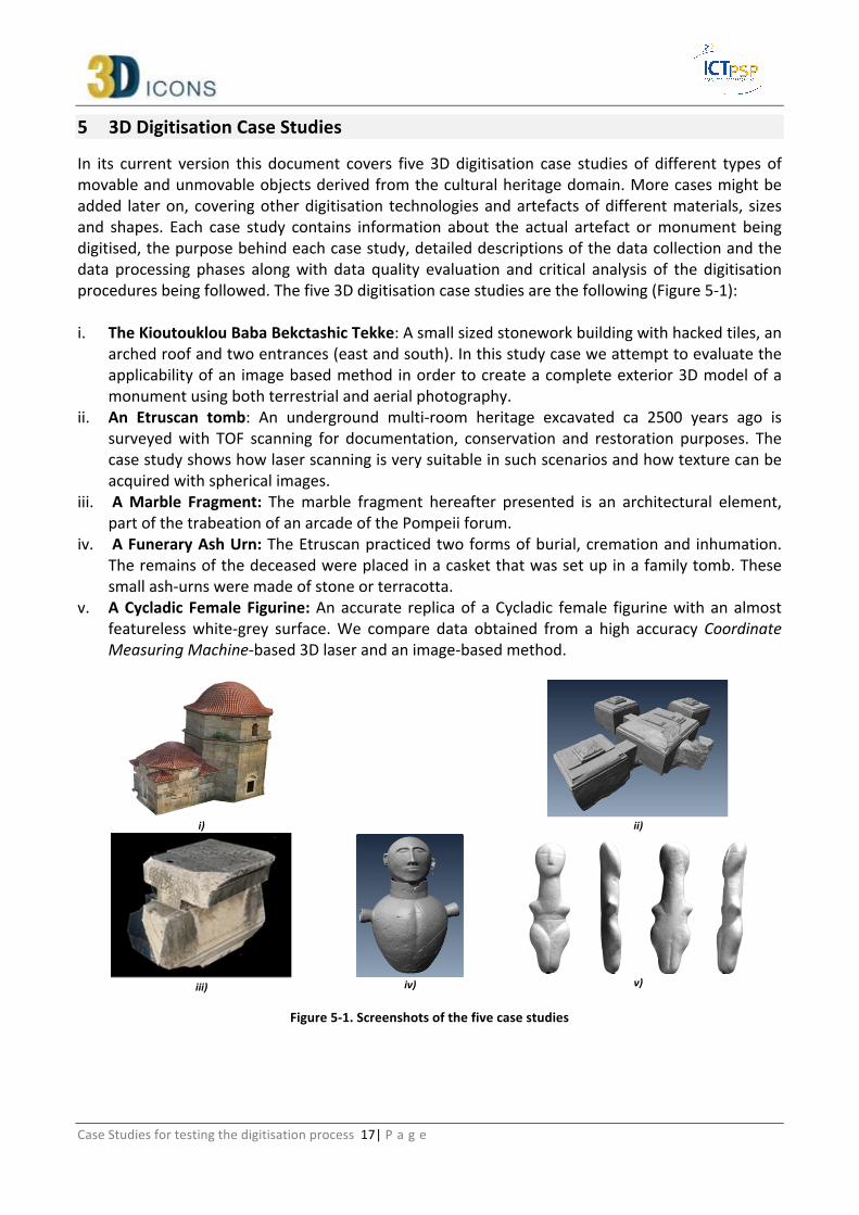
In its current version this document covers five 3D digitisation case studies of different types of movable and unmovable objects derived from the cultural heritage domain. More cases might be added later on, covering other digitisation technologies and artefacts of different materials, sizes and shapes. Each case study contains information about the actual artefact or monument being digitised, the purpose behind each case study, detailed descriptions of the data collection and the data processing phases along with data quality evaluation and critical analysis of the digitisation procedures being followed. The five 3D digitisation case studies are the following (Figure 5-‐1): i. The Kioutouklou Baba Bekctashic Tekke: A small sized stonework building with hacked tiles, an
arched roof and two entrances (east and south). In this study case we attempt to evaluate the applicability of an image based method in order to create a complete exterior 3D model of a monument using both terrestrial and aerial photography.
ii. An Etruscan tomb: An underground multi-‐room heritage excavated ca 2500 years ago is surveyed with TOF scanning for documentation, conservation and restoration purposes. The case study shows how laser scanning is very suitable in such scenarios and how texture can be acquired with spherical images.
iii. A Marble Fragment: The marble fragment hereafter presented is an architectural element, part of the trabeation of an arcade of the Pompeii forum.
iv. A Funerary Ash Urn: The Etruscan practiced two forms of burial, cremation and inhumation. The remains of the deceased were placed in a casket that was set up in a family tomb. These small ash-‐urns were made of stone or terracotta.
v. A Cycladic Female Figurine: An accurate replica of a Cycladic female figurine with an almost featureless white-‐grey surface. We compare data obtained from a high accuracy Coordinate Measuring Machine-‐based 3D laser and an image-‐based method.
i)
ii)
iii)
iv)
v)
Figure 5-‐1. Screenshots of the five case studies

Case Studies for testing the digitisation process 18| P a g e
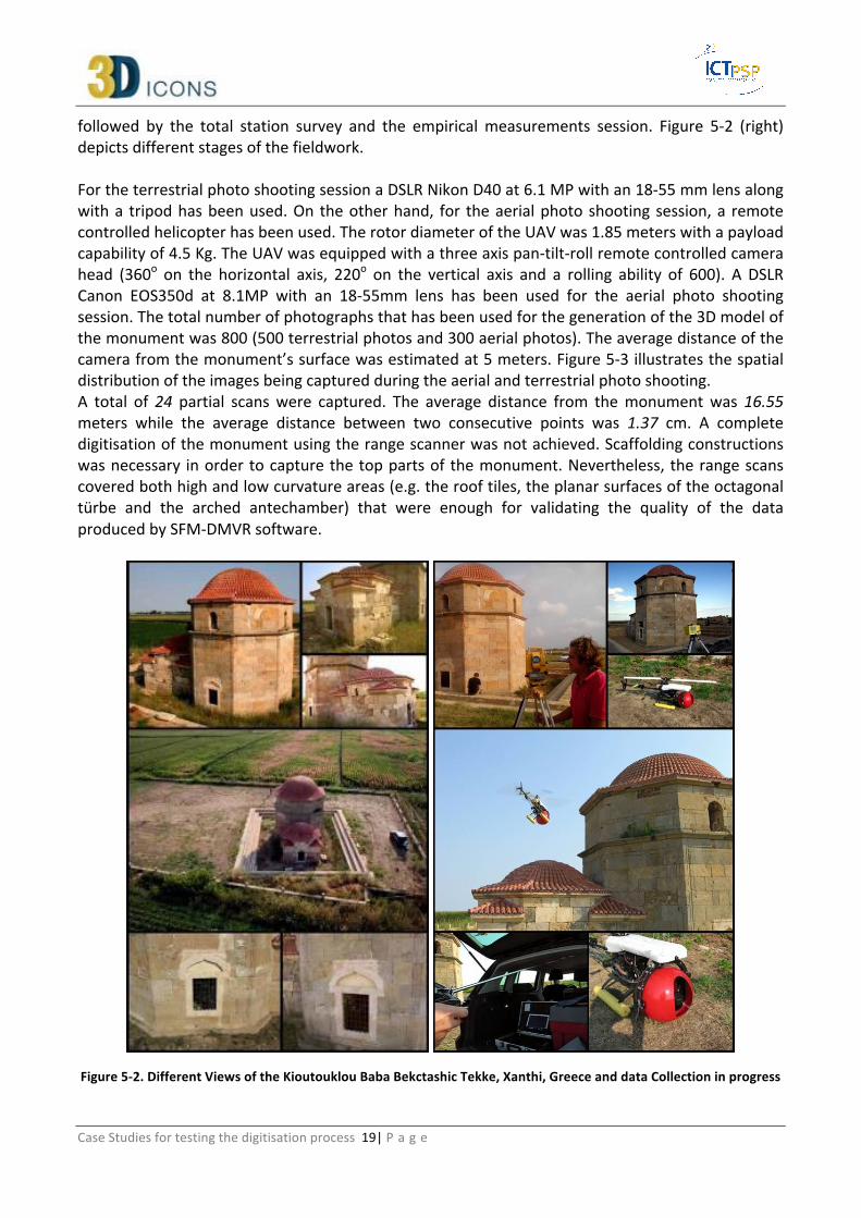
5.1 Case Study 1 – The Kioutouklou Baba Bekctashic Tekke The monument is located in the middle of a cultivable area on the west coast of the Vistonida lake in municipality of Xanthi, Greece (Figure 5-‐2 left). It is considered as one of the most important Ottoman monuments in the area and it may have been built in the late 15th century. It was possibly built on the ruins of an Orthodox Christian temple that was dedicated to Saint George Kalamitziotis [43]. According to Heath W. Lowry [45] the term tekke (gathering place for Dervishe) is erroneous as the monument is a tomb (türbe). Several conjectures have been made about the person buried in the monument [1]. Today, for the Muslims it is considered as the grave of a Whirling Dervishe named Kioutouklou Baba, while for the Christians it is a worshiping place of Saint George [45]. As shown in Figure 5-‐2, it is composed by an octagonal türbe (mausoleum) and an arched antechamber. The türbe has an arched roof and two windows (east and south) and it is made of stone with hacked tiles.
Possible 3D Digitisation Solutions 5.1.1 The current monument is placed in a flat area surrounded by fields used for agricultural purposes. There are no buildings around the monument and it considered an open access monument. Visitors of the area cannot be enclosed by barriers and thus during the data collection phase there is a chance of interruptions. The 3D digitisation of the monument could be performed using photogrammetric survey, range scanning or multi-‐image 3D reconstruction. The shape of the monument can be characterised as simple apart from the areas of the roof tiles. Consider the case of a project which requirement specifications indicate a low geometrical complexity 3D model for purely Web based visualisation purposes both 3D range scanning and multi-‐image 3D reconstruction methodologies will provide superfluous raw data. On the other hand, photogrammetric survey can be considered an option for such a case. Nevertheless, capturing the root tiles curvatures would be insufficient and thus synthetic 3D geometry texture mapped with real images would be required. The size and the position of the monument allow the efficient selection of viewpoints for photoshooting or range scanning all around the model. Nevertheless, in all three cases, the digitisation crew needs to consider the process of capturing the top of the monument which would require temporary scaffolding (3D range scanning) or an UAV for the image-‐based methodologies.
Purpose behind the specific case study 5.1.2 In this case study, we consider Agisoft PhotoScan as an all-‐to-‐one software solution for the production of digital 3D replicas of monuments. We attempt to evaluate the application of the method in order to create a complete exterior 3D model of a monument using both terrestrial and aerial photography. We compare the 3D mesh produced by the SFM-‐DMVR software against the data we captured from the same monument using other methods such as terrestrial 3D laser scanning, total station surveying and empirical distance measurements.
Collecting Data 5.1.3 The fieldwork was separated into five sessions. The first two involved the terrestrial and aerial photo shooting of the monument. Then, the terrestrial 3D laser scanning session took place
Case Studies for testing the digitisation process 19| P a g e
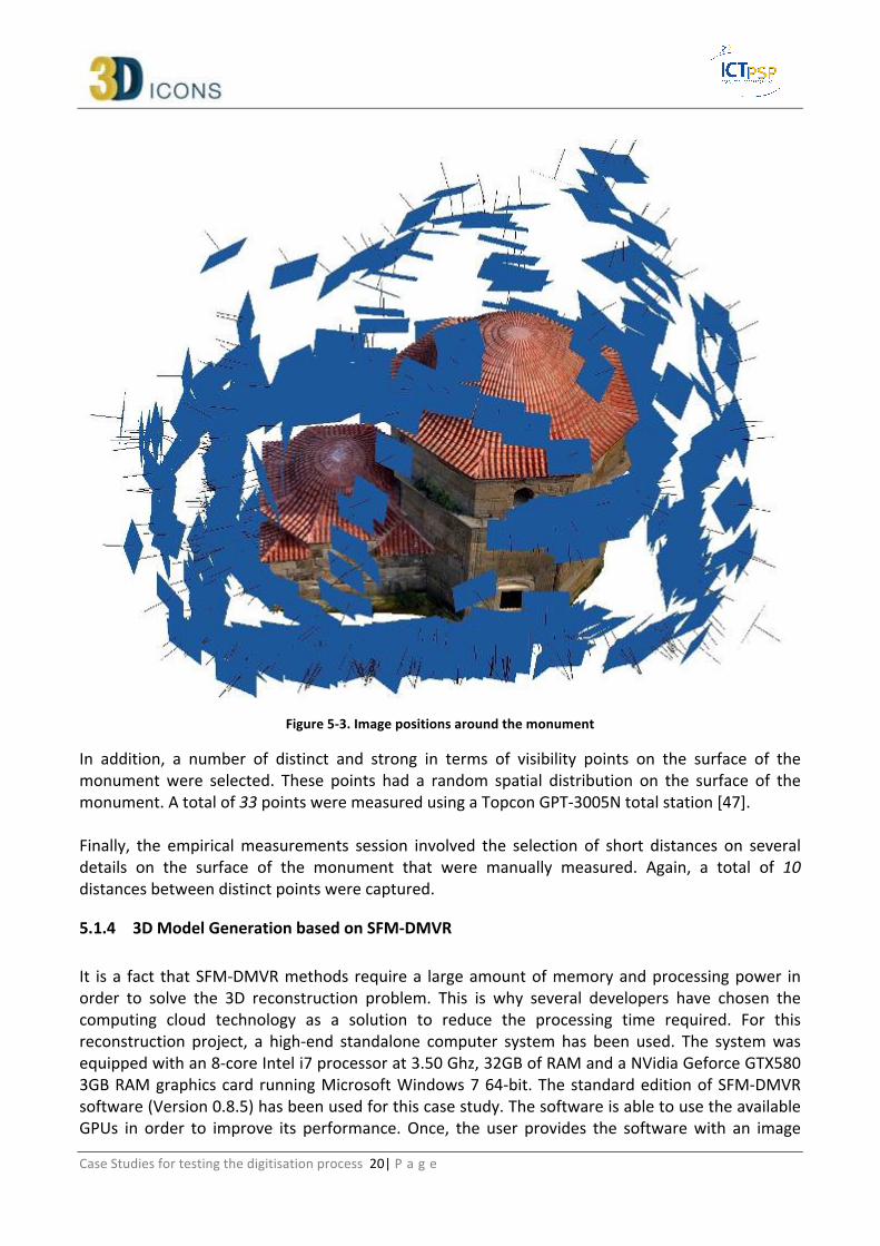
followed by the total station survey and the empirical measurements session. Figure 5-‐2 (right) depicts different stages of the fieldwork. For the terrestrial photo shooting session a DSLR Nikon D40 at 6.1 MP with an 18-‐55 mm lens along with a tripod has been used. On the other hand, for the aerial photo shooting session, a remote controlled helicopter has been used. The rotor diameter of the UAV was 1.85 meters with a payload capability of 4.5 Kg. The UAV was equipped with a three axis pan-‐tilt-‐roll remote controlled camera head (360o on the horizontal axis, 220o on the vertical axis and a rolling ability of 600). A DSLR Canon EOS350d at 8.1MP with an 18-‐55mm lens has been used for the aerial photo shooting session. The total number of photographs that has been used for the generation of the 3D model of the monument was 800 (500 terrestrial photos and 300 aerial photos). The average distance of the camera from the monument’s surface was estimated at 5 meters. Figure 5-‐3 illustrates the spatial distribution of the images being captured during the aerial and terrestrial photo shooting. A total of 24 partial scans were captured. The average distance from the monument was 16.55 meters while the average distance between two consecutive points was 1.37 cm. A complete digitisation of the monument using the range scanner was not achieved. Scaffolding constructions was necessary in order to capture the top parts of the monument. Nevertheless, the range scans covered both high and low curvature areas (e.g. the roof tiles, the planar surfaces of the octagonal türbe and the arched antechamber) that were enough for validating the quality of the data produced by SFM-‐DMVR software.
Figure 5-‐2. Different Views of the Kioutouklou Baba Bekctashic Tekke, Xanthi, Greece and data Collection in progress
Case Studies for testing the digitisation process 20| P a g e
Figure 5-‐3. Image positions around the monument
In addition, a number of distinct and strong in terms of visibility points on the surface of the monument were selected. These points had a random spatial distribution on the surface of the monument. A total of 33 points were measured using a Topcon GPT-‐3005N total station [47]. Finally, the empirical measurements session involved the selection of short distances on several details on the surface of the monument that were manually measured. Again, a total of 10 distances between distinct points were captured.
3D Model Generation based on SFM-‐DMVR 5.1.4 It is a fact that SFM-‐DMVR methods require a large amount of memory and processing power in order to solve the 3D reconstruction problem. This is why several developers have chosen the computing cloud technology as a solution to reduce the processing time required. For this reconstruction project, a high-‐end standalone computer system has been used. The system was equipped with an 8-‐core Intel i7 processor at 3.50 Ghz, 32GB of RAM and a NVidia Geforce GTX580 3GB RAM graphics card running Microsoft Windows 7 64-‐bit. The standard edition of SFM-‐DMVR software (Version 0.8.5) has been used for this case study. The software is able to use the available GPUs in order to improve its performance. Once, the user provides the software with an image

Case Studies for testing the digitisation process 21| P a g e
collection, the system almost automatically calibrates the cameras based on the EXIF information found in the images, aligns them into the 3D space and produces a complete and single 3D mesh using a dense multi-‐view reconstruction algorithm [48][49]. Then by fusing the depth maps that are contributed by each image that participates in the project’s solution, a complete 3D model of scene is created. As with all image based methods transparent or high reflectance surfaces are considered as challenging surfaces and produce poor reconstruction results. On the other hand, surfaces with high frequency of colour changes or rich texture features are considered as method-‐friendly. In our case study this happens to be true for almost the whole monument. Moreover, the software offers a number of predefined 3D reconstruction levels of detail (LOD). The level of detail affects the density of the reconstructed 3D mesh. Thus, although a higher resolution will produce a more detailed mesh, the processing time will be increased. Likewise, the amount of memory required to reconstruct the 3D scene and the amount of memory on the graphics card that is required to visualise the result in an adequate frame rate will be higher. Figure 5-‐4 depicts the different LODs of a specific detail on the monument’s exterior surface. In Figure 5-‐4, the colour of the mesh is given at the vertices level (Vertex Painted Mesh) and thus the higher the LOD, the higher the colour details on the model. Nevertheless, PhotoScan can also produce textured mapped meshes by blending parts of the image collection so that a realistic result can be achieved with low complexity 3D meshes. In addition, the total time required for the software to align the images into 3D space was 26 hours while Table 5-‐1 presents some of the most important properties of the different LOD reconstructed meshes. It should be noted that the computer system being used didn’t succeed in creating a complete ultra-‐high LOD 3D mesh from the given image selection. The complete reconstruction of the monument is presented in Figure 5-‐5.
Figure 5-‐4. Different LODs of the triangular mesh
LOD Num. of Vertices Num. of. Faces Distance
Between Vertices
Size (MB) (File Format:
PLY)
Total Processing Time
Lowest 1,567,136 3,049,047 55 mm 80 16 min. Low 6,347,734 12,381,156 25 mm 325 43 min. Medium 29,598,434 58,141,745 15 mm 1440 2 h. 46 min. High 161,537,781 317,769,170 3 mm 6554 17 h. 25 min.
Table 5-‐1. Properties of 3D model created at different LODs

Case Studies for testing the digitisation process 22| P a g e
Figure 5-‐5. Viewpoints of the reconstructed monument (Smooth Shaded Triangular Mesh and Vertex Painted
Medium Quality Triangular Mesh)
Different Methodologies Data Comparison and Results Evaluation 5.1.5 In order to evaluate the produced data, we have selected the medium 3D reconstruction resolution offered by the software as the properties of the produced mesh are considered the closest to the specifications and abilities offered by current average cost graphics card. A total of eleven single-‐view range scans were used as the ground truth data. The selection criteria for these range scans were: the practically parallel positioning of the scanner’s sensor plane against the monument’s large planar surfaces and the relatively low average distance between the scanner’s position and the monument. The 3D data comparison pipeline that we followed included open source software such as Meshlab [50] and CloudCompare [51]. Meshlab was used to align the partial scans of the range scanner with the 3D model produced by the SFM-‐DMVR software. On the other hand, the CloudCompare software was used to estimate the surface deviation between the SFM-‐DMVR data and the range scanner data. We chose to compare single-‐view range scans against the SFM-‐DMVR model. This resulted in more accurate surface deviation measurements between the two data types. An alignment and merging procedure of the different range scans using an algorithm such as the
Case Studies for testing the digitisation process 23| P a g e
iterative closest point (ICP) would build-‐up the surface deviation error. This is due to the fact that ICP is attempting to minimise (distribute) the alignment error between all the overlapping neighbouring meshes. Nevertheless, the ICP algorithm, implemented in Meshlab, has been used to align each single-‐view range scan with the SFM-‐DMVR triangular mesh model. In order to compare the two data types, the cloud-‐to-‐mesh distance function offered by CloudCompare was selected. This function is considered more robust to local noise when compared to the cloud-‐to-‐cloud distance option. The cloud-‐to-‐mesh distance function computes the distances between each vertex of the point cloud to the nearest triangle of the mesh surface. The distance between the two is calculated as follow. In cases where the orthogonal projection of the vertex lies inside the surface defined by a triangle, then the distance between the vertex and its point-‐of-‐intersection on the surface is calculated. Otherwise, the software estimates the distances between the vertex and its projection to the nearest edge or to the nearest vertex of the triangle [52]. In our experiments, the SFM-‐DMVR model was always used as the mesh and each range scan as a point cloud. Illustrations of the colour encoded surface deviations of the monument’s exterior surfaces along with tables containing mean distances and standard deviation can be found at Appendix 1. From the data comparison, it obvious that SFM-‐DMVR methods have issues when reconstructing surfaces of low features. The low frequency of colour alternations on the roof tiles in conjunction with the bad lighting in the hollow areas between every alternate roof tile row composes a challenging, for SFM-‐DMVR methods, surface. For further assessment of the SFM-‐DMVR data, we compared a number of distance measurements between specific feature points on both data types (range scans and SFM-‐DMVR mesh) to the measurements that we have previously carried out on the actual monument using a total station. The feature points were selected based on the fact that they were apparent and easy to be recognised on the monument’s surface. The distance differences are presented again in Appendix 1. The procedure of manually selecting a point on the 3D data introduces an accuracy ambiguity. Nonetheless, the quality of the triangulated mesh as well as the range scanner’s data provided an acceptable visualisation of these features points. Furthermore, we attempted to verify a set of empirical measurements that have been previously performed on the surface of the monument between fine details on the surface of the monument. These distances varied between 7cm and 30cm. Again, using Meshlab, we performed the same distance measurements on the PhotoScan mesh. The results are presented in Appendix 1 and are found to be acceptable for a digitisation project that aims in visualising 3D models of monuments over the Web. All the previous experiments contributed on verifying that the SFM-‐DMVR model does not contain proportional errors. Nevertheless, SFM-‐DMVR methods fail to reconstruct areas of low frequency colour changes and lack of strong features. The results on such challenging areas can always be improved by taking additional pictures from a closer distance. In our case this wasn’t possible due to the size of the UAV and the already low safety distance from the monument. Moving around the monument with a digital camera is more efficient in relation to moving a range scanner but again a reduction in the efficiency factor of the method should be considered in terms of number of images against the surface area being covered and processing time required for the automated image-‐based 3D reconstruction.

Case Studies for testing the digitisation process 24| P a g e
3D Data Post Processing 5.1.6 Below, we present a simple 3D data post processing example based the data derived from the previous case study. The purpose of this post processing example is the reduction of the geometrical complexity of the model while having a subjectively acceptable visual result. The high quality reconstructed model counts more than 300 million polygons, which is an extremely large number even for modern 3D graphics accelerators. Meshlab was used in order to simplify (decimate) the mesh into a more adequate, for common hardware, version. This was achieved using the quadric edge collapse decimation function. A lightweight version of the 3D model was produced counting 80,000 triangles (Figure 5-‐6). Then, the low polygon model was imported into PhotoScan and was textured map automatically using the previously aligned images data set. A subjective comparison of the different decimation levels can be performed with the help of the figure below (Figure 5-‐7). The successful and accurate automatic texturing of the low polygon model indicates a low surface deviation between the two different in resolution versions of the 3D mesh.
a) 300M polygon model with bitmap texture map
b) 80K polygon model with bitmap texture map
Figure 5-‐6. Subjective comparison between of different geometrical complexity models

Case Studies for testing the digitisation process 25| P a g e
Figure 5-‐7. Wireframe rendering of the same model using 80,000 (left) 300,000 (right) and 34 million triangles (bottom).
Moreover, it should be noted that apart from removing the unwanted parts from the surrounding area and the production of the simplified versions from the initial data no further processing was applied on the raw data.
Metadata Creation 5.1.7This section will be completed after the schema for the 3D-‐ICONS is finalized and tested in WP.6.1 and WP 6.2
3D Data Formats for Publication 5.1.8This section will be completed after the 3D-‐ICONS deliverable in WP 5.1 is finalized

Case Studies for testing the digitisation process 26| P a g e
Conclusions 5.1.9 In this case study, we have evaluated the quality of the data produced by a low-‐cost commercial 3D reconstruction software that is based on the Structure-‐from-‐Motion and Dense Multi-‐View 3D Reconstruction techniques. The data evaluation phase indicated that for monuments with feature-‐rich surfaces under appropriate lighting conditions, high quality results can be achieved by a large set of images. A high performance computer system in terms of available memory, processing power and graphics card capabilities is required in order to solve similar 3D reconstruction projects. In the case of Kioutouklou Baba Bekctashic Tekke, the produced data clearly indicate that a SFM-‐DMVR software can provide high quality results. But as SFM-‐DMVR belong to the image-‐based techniques, the quality of the produced data are highly correlated and depended on the unavoidable procedure of identifying corresponding points in large sets of images that depict the same part of the scene from different viewpoints. In addition, the quality of the produced 3D model depicts the applicability of the SFM-‐DMVR methods in low budget digitisation or documentation projects. The semi-‐automated functionality of the software composes a low-‐cost solution that also requires a low knowledge overhead by the end-‐user. On the other hand, digitising the monument with a terrestrial range scanner requires a different digitisation plan. Range scanners do not require visual cues in order to extract depth information and thus they can provide accurate 3D data even from a single viewpoint. However, it is impossible to acquire a complete digital model of a monument just from a single scan position-‐viewpoint, unless it is just a very smooth relief that faces the scanner. In most cases, multiple scans captured from various positions around the monument are necessary. Although their number is by far lesser than those of the image-‐based 3D reconstruction the actual acquisition time of those partial range scans is much greater3. The reason of this is that still terrestrial range scanners are still bulky and slow in terms of acquisition devices when compared with a digital camera. In addition, they require being motionless on a tripod for a period of time, measuring from minutes up to hours. Subsequently, acquiring data with a range scanner can be considered as a much more challenging task, involving in some cases temporary scaffolding construction and potentially dangerous working conditions in order to capture the complete structure of a monument.
Figure 5-‐8. 3D Digitisation in progress using a terrestrial 3D range Scanner – Examples of using of temporary
scaffolding (Image courtesy [53]-‐[56])
3 Acquisition times are related with the actual range scanner capabilities and the sampling rate required in each case.

Case Studies for testing the digitisation process 27| P a g e
The acquisition of multiple partial scans is always followed by the processes of data clean up, partial scan alignment and merging. The raw data produced by a range scanner are usually dense coloured point clouds. Some of the most usual problems found in the raw data of a range scanner are noisy points that surround sharp edges, occlusion of structures (shadowing) and variable sampling rate within the same scan due to different distances between the parts of the monument and the range scanner. The partial scans can also include special residual points that are geo-‐referenced and are placed by the members of the digitisation team in order to support the alignment procedure. For the simplification of the partial scans alignment, there are also range-‐scanning systems that provide information about their geo-‐referenced position. Thus, the alignment of the partial scans is a semi-‐automated procedure that can be considered as an error-‐prone step due to the manual identification and selection of common points in the overlapping areas of the partial scans. In fact, a misalignment can occur due to errors produced either by the user or the algorithm. After the alignment, all the partial range scans compose again a raw point cloud (a superset of the partial scans) that requires further processing. The overlapping areas depict the same surface area from a different position and thus the same surface is described by point clouds of varying quality properties. In order to achieve the optimum results from the acquired data, some overlapping points must be removed. Usually for each scan set, the points that are beyond scanners’ optimal range and those that exhibit extreme vector normal deviation from scanners’ position can be discarded. Furthermore, the process of excluding problematic data out of the raw datasets is common for both SFM-‐DMVR methods and terrestrial range scanning. Due to the fact that 3D digitisations using a laser scanner can be achieved by acquiring data by far less placements of the digitisation device around the subject, renders data clean-‐up for laser scanning as a much more time efficient procedure compared to the equivalent in SFM-‐DMVR methods. Moreover, one of the advantages of methodologies, such as photogrammetry and surveying using a total station and empirical measurements, over methods such as terrestrial range scanning and SFM-‐DMVR, is that they produce data that don’t have require to be cleaned. However, these methodologies are characterised by their incompetence to provide dense data. On the other hand, equally important to the digitisation of the 3D structure of a monument is its colour information. Colour information can be acquired using a digital camera. In the case of SFM-‐DMVR capturing colour information is considered trivial. The content of the same digital images that are used to create the 3D geometry can be used to extract the colour information. Consequently, one can comprehend the absolute correlation between geometrical and colour information. However, in the case of 3D range scanners, the above correlation cannot be taken always for certain. In order for a range scanner to acquire colour information a digital camera is necessary. This digital camera has to be calibrated and registered in relation to the laser source of the range scanner, in order to achieve an alignment between the colour and the geometry. Nowadays, many commercial range scanners are equipped with such digital cameras that are positioned internally on the same axis with the laser source and thus resulting in a more accurate alignment between geometrical and colour information. As the image resolution and colour quality of the internal cameras are not always adequate, there are procedures that can be followed to calibrate an external digital camera of higher quality.

Case Studies for testing the digitisation process 28| P a g e
Furthermore, all 3D range scanners with an internal digital camera that has a shifted point of view from that of the range sensor, are prone to colour information ghosting, due to the different perspective projections of the same real world scene. Colour information bleeding is another common problem found in many range scanners and yields on the different sampling resolution between the digital camera and the range scanning subsystem. In addition, colour information quality is also affected by the optics and image sensor properties and characteristics of the camera subsystem. Low light conditions are usually a case where many commercial range scanners fail to deliver adequate colour information. Nevertheless, capturing 3D structures in low light conditions is considered as one of the greatest advantages of range scanners against the other acquisition methods. Range scanners can actually acquire geometry and reflectivity properties of the surface in conditions of complete darkness. This characteristic renders laser scanners as the most adequate choice for the digitisation of subjects such as caves, dark areas and poorly lit indoor environments. Then again, SFM-‐DMVR methodologies can be used in such cases as well, however proper lighting conditions need to be implemented and thus results in additional costs.
5.2 Case Study 2 – Etruscan tomb
The heritage and the selected 3D recording technique 5.2.1 There are different Etruscan heritage sites in the centre of Italy dating back to VII-‐IV century B.C. and some of these are recognized as an UNESCO World Heritage site. Most of the sites consist of necropolis with hundreds of underground frescoed tombs, monumental, cut in rock and often topped by impressive tumuli (burial mounds). Many tombs feature carvings on their walls, others have paintings of outstanding quality, still visible and partly preserved. Most of these tombs are inaccessible to the visitors therefore the recorded and processed 3D data are also used to create digital contents for virtual visits, museum exhibitions, better access and communication of the heritage information. Therefore an accurate and photorealistic result is expected to guarantee a correct and digital documentation as well as virtual or remote access to otherwise hardly reachable heritage closed to the public for preservation reasons. The produced 3D models are also used for analyses and investigations on the tomb geometries, for archaeological documentation, digital preservation and to validate archaeological hypotheses or to make new ones. The Etruscan tombs and ruins constitute a unique and exceptional testimony to the ancient Etruscan population, the only urban civilization in pre-‐Roman Italy. Moreover, the depicted daily life in the frescoed tombs, many of which are replicas of Etruscan houses, is a unique testimony to this vanished culture. Many of the tombs represent types of buildings that no longer exist in any other form. The digital recording of an Etruscan tomb is a complex task and it should follow some fundamental steps (Figure 5-‐9) in order to satisfy the project requirements. The 3D recording of heritage sites frequently requires a multi-‐disciplinary approach with multiple 3D recording techniques to take into account different and specific characteristics of these sites. For example, the frescoes inside some of the Etruscan tombs are particularly sensitive to any micro-‐climate variation (humidity, temperature, vibrations). This specification involves special constraints and care for the data acquisition stage such as a limited number of persons inside the tomb, the use of cool lights during image acquisition and of course only non-‐contact surveying techniques, just to mention some of them.

Case Studies for testing the digitisation process 29| P a g e
The typical geometric configuration of an Etruscan tomb features a down-‐hill stairway (dromos) and then different chambers connected by narrow corridors. Many tombs have also niches or sarcophagus inside their rooms that produce many perspective occlusions. In surveying it is well known that redundancy is sometimes the only way to find gross errors and get reliable and precise results. But in some situations, the cramped spaces do not allow for any redundancy of data. If not carefully planned, the 3D survey can lead to unreliable results due to the weak geometry of the structures. A surveying techniques like photogrammetry (based on the triangulation principle and requiring overlapping images, hence multiple positions to measure a 3D point), is not suggested due to the multiple occlusions, narrow spaces, smoothed geometry, often lack of texture as well as bad illumination conditions. Photogrammetry can be coupled with a topographic survey in order to provide the coordinates of some reference/check points for the image orientation step. But this would require long time in the tomb and also the marking of natural features / corners. For all these reasons, excluding some specific analyses that require dedicated sensors such as multi-‐spectral cameras, the suggested 3D surveying technique for this kind of underground structures is 3D laser scanning. TOF or phase-‐shift scanners are active sensors able to measure a 360 degrees point cloud from a single station (monoscopic technique) even in case of dark environment. High resolution digital images were separately acquired with a calibrated camera for texture mapping and frescoes documentation.
Figure 5-‐9. The pipeline that needs to be followed when working at the digital documentation and 3D modelling of heritage scenes and objects.
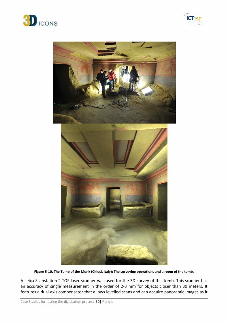
3D surveying and modelling 5.2.2 The surveyed tomb reported in this example is the Tomb of the Monkey which dates back to V century B.C. and is located in Chiusi (Tuscany, Italy). The tomb, excavated in the hard sand, has four rooms. The main room, bigger respect to the others, is in a central position and measures 5 x 4 meters in planimetry, the others rooms, smaller, measure ca. 3 x 3 meters and are connected to the main one through corridors that are about 0.8 x 2 m in planimetry. The height of the tomb rooms does not exceed 3 meters and most of the sealing feature bass-‐reliefs. Inside the rooms some burial beds are placed closed the walls which are still painted with reddish colour (Figure 5-‐10).
Case Studies for testing the digitisation process 30| P a g e
Figure 5-‐10. The Tomb of the Monk (Chiusi, Italy): The surveying operations and a room of the tomb.
A Leica Scanstation 2 TOF laser scanner was used for the 3D survey of this tomb. This scanner has an accuracy of single measurement in the order of 2-‐3 mm for objects closer than 30 meters. It features a dual-‐axis compensator that allows levelled scans and can acquire panoramic images as it
Case Studies for testing the digitisation process 31| P a g e
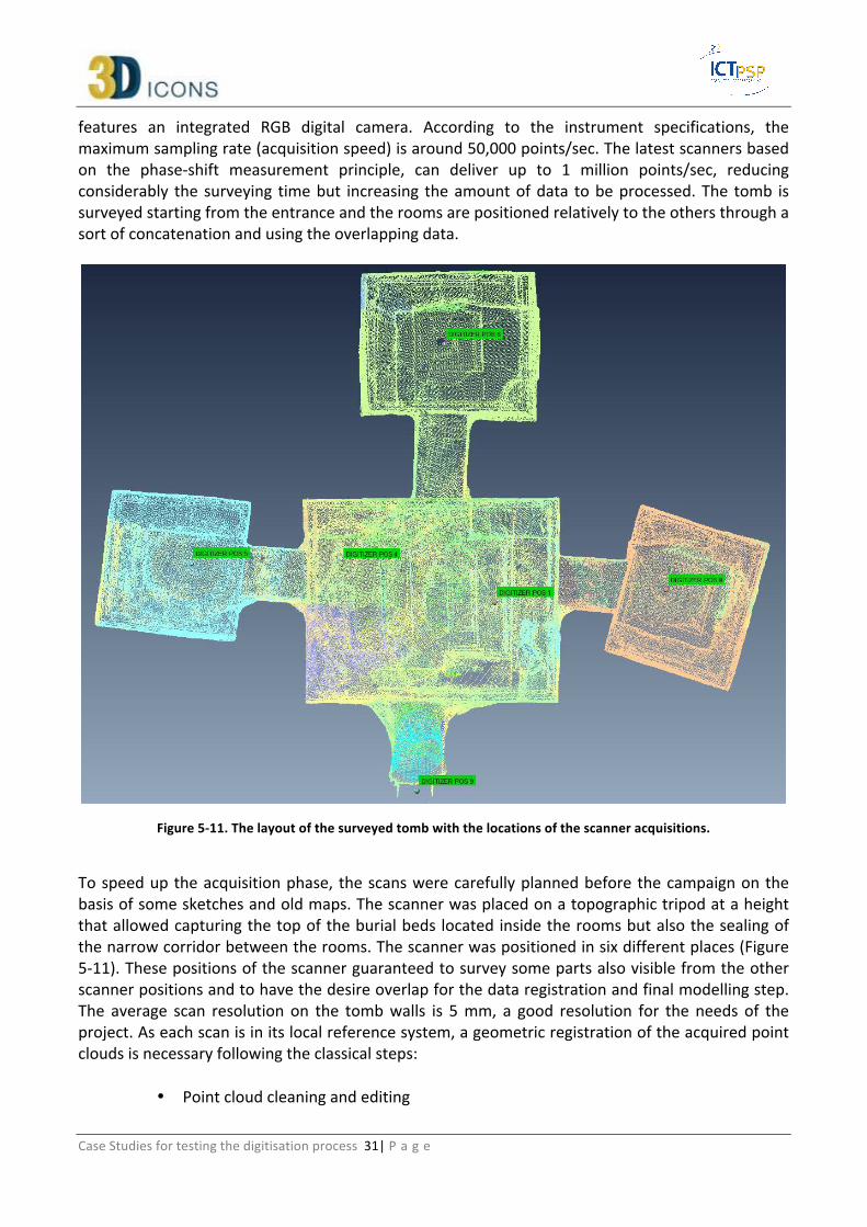
features an integrated RGB digital camera. According to the instrument specifications, the maximum sampling rate (acquisition speed) is around 50,000 points/sec. The latest scanners based on the phase-‐shift measurement principle, can deliver up to 1 million points/sec, reducing considerably the surveying time but increasing the amount of data to be processed. The tomb is surveyed starting from the entrance and the rooms are positioned relatively to the others through a sort of concatenation and using the overlapping data.
Figure 5-‐11. The layout of the surveyed tomb with the locations of the scanner acquisitions.
To speed up the acquisition phase, the scans were carefully planned before the campaign on the basis of some sketches and old maps. The scanner was placed on a topographic tripod at a height that allowed capturing the top of the burial beds located inside the rooms but also the sealing of the narrow corridor between the rooms. The scanner was positioned in six different places (Figure 5-‐11). These positions of the scanner guaranteed to survey some parts also visible from the other scanner positions and to have the desire overlap for the data registration and final modelling step. The average scan resolution on the tomb walls is 5 mm, a good resolution for the needs of the project. As each scan is in its local reference system, a geometric registration of the acquired point clouds is necessary following the classical steps:
• Point cloud cleaning and editing
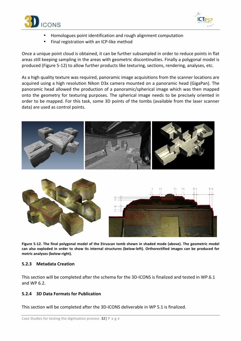
Case Studies for testing the digitisation process 32| P a g e
• Homologues point identification and rough alignment computation • Final registration with an ICP-‐like method
Once a unique point cloud is obtained, it can be further subsampled in order to reduce points in flat areas still keeping sampling in the areas with geometric discontinuities. Finally a polygonal model is produced (Figure 5-‐12) to allow further products like texturing, sections, rendering, analyses, etc. As a high quality texture was required, panoramic image acquisitions from the scanner locations are acquired using a high resolution Nikon D3x camera mounted on a panoramic head (GigaPan). The panoramic head allowed the production of a panoramic/spherical image which was then mapped onto the geometry for texturing purposes. The spherical image needs to be precisely oriented in order to be mapped. For this task, some 3D points of the tombs (available from the laser scanner data) are used as control points.
Figure 5-‐12. The final polygonal model of the Etruscan tomb shown in shaded mode (above). The geometric model can also exploded in order to show its internal structures (below-‐left). Orthorectified images can be produced for metric analyses (below-‐right).
Metadata Creation 5.2.3 This section will be completed after the schema for the 3D-‐ICONS is finalized and tested in WP.6.1 and WP 6.2.
3D Data Formats for Publication 5.2.4 This section will be completed after the 3D-‐ICONS deliverable in WP 5.1 is finalized.

Case Studies for testing the digitisation process 33| P a g e
5.3 Case Study 3 -‐ A marble fragment The marble fragment presented in this case study is an architectural element, part of the trabeation of an arcade of the Pompeii forum (Figure 5-‐15). Its main dimensions are about 2 meters by 0.5 meter in planimetry and 1.5 meter in height. The shape of the object is quite simple but has some interesting fine details in the order of few millimetres (surface characterization). The object is located inside the forum within the area open to the visitors of the archaeological site. Many fragments with similar characteristics are spread over the forum area.
The heritage and the selected 3D recording technique 5.3.1 The marble fragment hereafter presented is an architectural element, part of the trabeation of an arcade of the Pompeii forum. Its main dimensions are about 2 meters by 0.5 meter in planimetry and 1.5 meter in height. The shape of the object is quite simple but has some interesting fine details in the order of few millimetres (surface characterization). The object is located inside the forum within the area open to the visitors of the archaeological site. Many fragments with similar characteristics are spread over the forum area. These types of objects are normally surveyed and modelled using a terrestrial photogrammetric workflow. The procedure is almost entirely manual using monoscopic plotting/reconstruction. The main reasons behind this choice can be summarized as follows:
• the object material is known to be problematic if surveyed using laser scanners instruments, both triangulation or distance meter scanners (time of flight or shift based);
• the object is located outside under the sun light, fringe projection system are difficult to use (most time useless) in strong illuminated environment;
• the object is located in the visitors area and cannot not be enclosed by barriers, a fast acquisition method is therefore desirable;
• the simple geometrical shape of the object allows an easy reconstruction with few 3D points and polygons.
Figure 5-‐13. A marble fragment which needs to be digitally modelled for virtual replica, web application and
archaeological analysis.
3D surveying and modelling 5.3.2 The 3D acquisition/reconstruction process was accomplished through a well-‐established acquisition protocol (see Appendix 2). The photogrammetric survey was specifically planned on the basis of the required accuracy and LoD. The geometry of the 3D model had to be very simple to guarantee a

Case Studies for testing the digitisation process 34| P a g e
fast visualization in virtual reality environments and for online publication but, at the same time, the conservators must still have a detailed photographic and geometric documentation of each side of the finding. The employed camera was a Canon 20D that features a pixel size of 6.4 μm and was coupled used with a lens whose principal distance c was 20 mm. For the marble fragment, a good compromise for planning the image acquisition was found with a Ground Sample Distance (GSD) of 3 mm that can guarantee the visibility of details needed in 1:20 maps/plans. This parameter guided the planning stage as to assure such a geometric resolution. Images had to be taken closer than a limit distance beyond which the GSD became larger than the one desired. The marble fragment was imaged in 15 convergent images acquired at an average distance of ca 2 meters with the digital camera previously calibrated in laboratory by means of a photogrammetric bundle adjustment and using a 3D test-‐field. A yardstick (ruler) was also placed in the scene in order to give a scale to the photogrammetric project. For this class of objects and for the needs of the project, the image processing is carried out using an interactive monoscopic approach (e.g. Photomodeler, Iwitness, etc.). Corresponding points are marked in the images following the classical photogrammetric steps: (i) Image orientation: This stage computes the camera poses (exterior orientation) through some analytical steps also known as relative orientation followed by an optimization process called bundle adjustment. The image correspondences selected by the operator are the observation used to compute the unknown camera poses (Figure 5-‐16).
Figure 5-‐14. Image orientation: camera poses respect to the 3D model
(ii) Datum definition: This stage gives metric characteristics to the solution computed in the previous step (usually in an arbitrary scale). Two approaches can be used to create metric results:
1. At least one distance must be assigned to two object points visible on the images. For this reason it is common to use scale bars, yardsticks or targets measured with topographic method that are visible in the images to scale the photogrammetric survey. In some cases, distances between natural features can be used when they are well distinguishable in the images (i.e. they have a good contrast and the shape is unchanging when seen from different points of view – example: bricks intersections). More than one distance can be
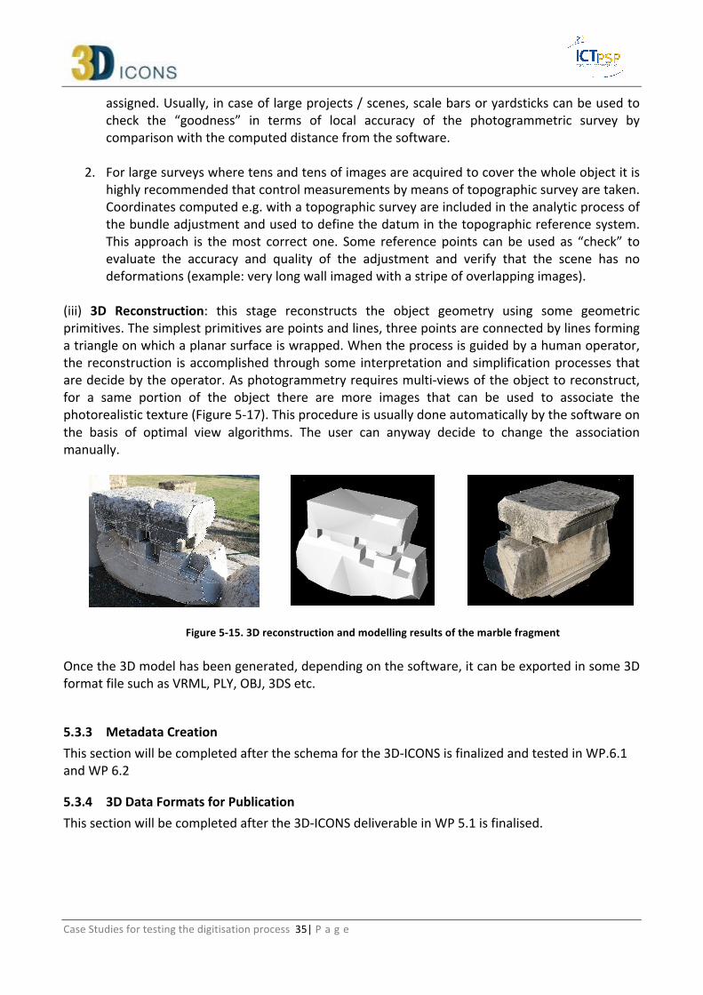
Case Studies for testing the digitisation process 35| P a g e
assigned. Usually, in case of large projects / scenes, scale bars or yardsticks can be used to check the “goodness” in terms of local accuracy of the photogrammetric survey by comparison with the computed distance from the software.
2. For large surveys where tens and tens of images are acquired to cover the whole object it is highly recommended that control measurements by means of topographic survey are taken. Coordinates computed e.g. with a topographic survey are included in the analytic process of the bundle adjustment and used to define the datum in the topographic reference system. This approach is the most correct one. Some reference points can be used as “check” to evaluate the accuracy and quality of the adjustment and verify that the scene has no deformations (example: very long wall imaged with a stripe of overlapping images).
(iii) 3D Reconstruction: this stage reconstructs the object geometry using some geometric primitives. The simplest primitives are points and lines, three points are connected by lines forming a triangle on which a planar surface is wrapped. When the process is guided by a human operator, the reconstruction is accomplished through some interpretation and simplification processes that are decide by the operator. As photogrammetry requires multi-‐views of the object to reconstruct, for a same portion of the object there are more images that can be used to associate the photorealistic texture (Figure 5-‐17). This procedure is usually done automatically by the software on the basis of optimal view algorithms. The user can anyway decide to change the association manually.
Figure 5-‐15. 3D reconstruction and modelling results of the marble fragment
Once the 3D model has been generated, depending on the software, it can be exported in some 3D format file such as VRML, PLY, OBJ, 3DS etc.
Metadata Creation 5.3.3This section will be completed after the schema for the 3D-‐ICONS is finalized and tested in WP.6.1 and WP 6.2
3D Data Formats for Publication 5.3.4This section will be completed after the 3D-‐ICONS deliverable in WP 5.1 is finalised.

Case Studies for testing the digitisation process 36| P a g e
5.4 A funerary ash urn The digital recording of an Etruscan ash urn is part of a project that aimed to digitally document and preserve the heritage object and realise virtual copies for remote access. The Etruscan practiced two forms of burial, cremation and inhumation. The remains of the deceased were placed in a casket that was set up in a family tomb. These small ash-‐urns were made of stone or terracotta. The urn styles range from biconical (vase shaped) to miniature hut style to the canopic style with human figures or heads on their lids. Sarcophagi and urns were placed in the tombs with other burial items necessary for the afterlife. The ash urn used in this case study is made of terracotta and measures about 50 cm in height and has a maximum diameter of about 30 cm. A head made of the same material is used as cap of the vase. Small cracks are present on its surface whose colour is uniform and brownish.
The heritage and the selected 3D recording technique 5.4.1 The rounded shape of the artefact, its texture and its small details suggested to employ a triangulation-‐based scanner in order to achieve very highly detailed geometric results and overcome lack of texture. The object is thus surveyed with a ShapeGrabber PLM Series using the SG102 Scan Head and a 600 mm arm. The instrument’s accuracy mainly depends on the mounted head and the geometric resolution can be as high as 20 microns. The accuracy in depth measurement is better than 0.1 mm.
3D surveying and modelling 5.4.2 The ash urn was located in a depository in the museum of Chianciano Terme (Italy). The urn and the head were positioned on a potter’s wheel whose rotation could be locked. The distance between the laser scanner and the object was approximately 40-‐50cm. For each partial scan the scanner and the object were left still, then the urn rotated and the wheel locked again for each successive partial scan. This expedient was necessary to limit the scanner movements and maximize the acquisition speed. As the sampling step of the scanner (geometric resolution) was set at 100 microns, particular attention was paid to avoid possible shakes or oscillations of the instruments which would have cause errors in the acquired data. A total of 22 scans (Figure 5.16) of the vase and the head were acquired with an average number of points per scan of about 340,000 points. The total number of points was about 7.5M with an average resolution of 1pt/0.4 mm. All the point clouds were aligned using an ICP method and finally a mesh was created and textured (Figure 5-‐14).

Case Studies for testing the digitisation process 37| P a g e
Figure 5-‐13. Some scans acquired with the triangulation-‐based scanner setting a resolution of 100 micron.
Figure 5-‐14.The geometric 3D model of the ash urn shown in shaded and textured model.
Metadata Creation 5.4.3 This section will be completed after the schema for the 3D-‐ICONS is finalized and tested in WP.6.1 and WP 6.2.
3D Data Formats for Publication 5.4.4 This section will be completed after the 3D-‐ICONS deliverable in WP 5.1 is finalized.
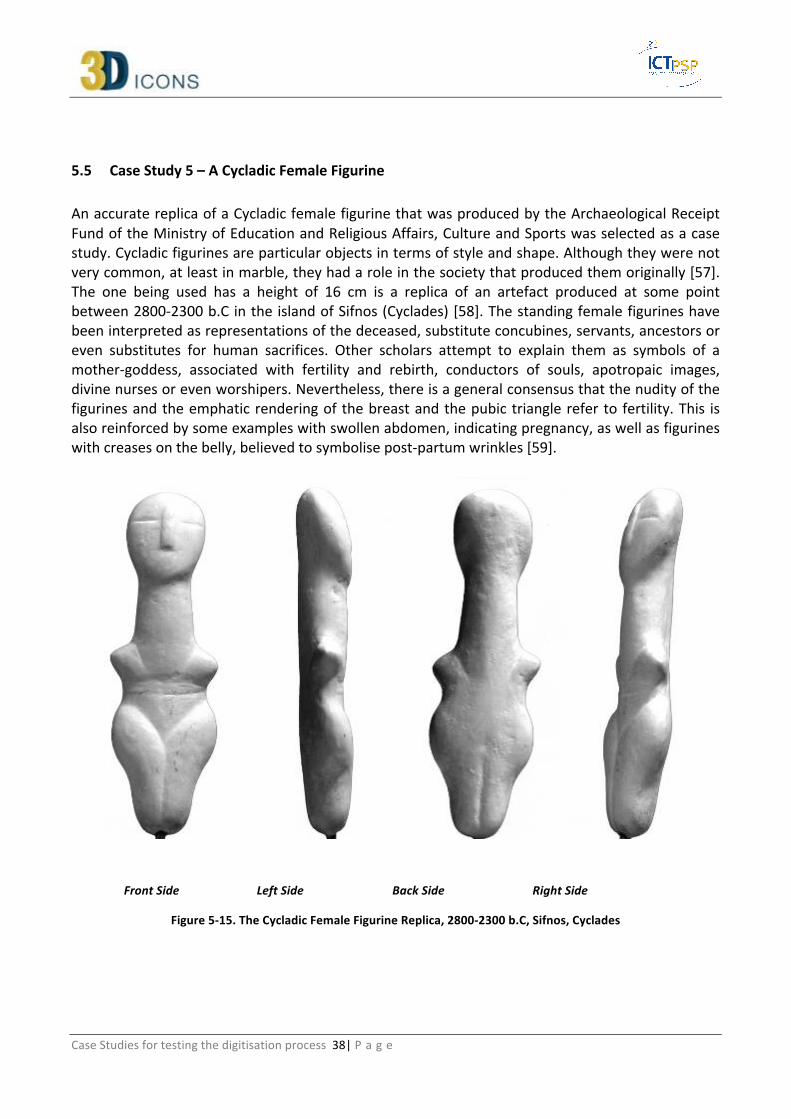
Case Studies for testing the digitisation process 38| P a g e
5.5 Case Study 5 – A Cycladic Female Figurine An accurate replica of a Cycladic female figurine that was produced by the Archaeological Receipt Fund of the Ministry of Education and Religious Affairs, Culture and Sports was selected as a case study. Cycladic figurines are particular objects in terms of style and shape. Although they were not very common, at least in marble, they had a role in the society that produced them originally [57]. The one being used has a height of 16 cm is a replica of an artefact produced at some point between 2800-‐2300 b.C in the island of Sifnos (Cyclades) [58]. The standing female figurines have been interpreted as representations of the deceased, substitute concubines, servants, ancestors or even substitutes for human sacrifices. Other scholars attempt to explain them as symbols of a mother-‐goddess, associated with fertility and rebirth, conductors of souls, apotropaic images, divine nurses or even worshipers. Nevertheless, there is a general consensus that the nudity of the figurines and the emphatic rendering of the breast and the pubic triangle refer to fertility. This is also reinforced by some examples with swollen abdomen, indicating pregnancy, as well as figurines with creases on the belly, believed to symbolise post-‐partum wrinkles [59].
Front Side Left Side Back Side Right Side
Figure 5-‐15. The Cycladic Female Figurine Replica, 2800-‐2300 b.C, Sifnos, Cyclades

Case Studies for testing the digitisation process 39| P a g e
Possible 3D Digitisation Solutions 5.5.1 The current artefact’s morphological features and surface is considered friendly for a variety of digitisation methods. It can be successfully digitised in three dimensions by using a 3D laser scanner, a shape-‐from-‐structured light scanner, multi-‐image 3D reconstruction software or even an obsolete shape-‐from-‐silhouette 4 system. Considering that all methodologies are implemented as portable systems, all of them can be applied in-‐situ (e.g. a museum where the artefact might be kept). If the presence of the digitisation crew in the museum is considered an issue in terms of time, then a shape-‐from-‐structured light system is more preferable choice in terms data capturing time and quality of raw data. Capturing an image data set that depicts the object from different viewpoints would also be an applicable choice in terms of data capturing time. In terms of geometrical accuracy modern laser scanning systems still offer higher detail although state-‐of-‐the-‐art shape-‐from-‐structured light systems are based on high definition projectors. Apart from the shape-‐from-‐silhouette method that is considered almost automated in terms of producing a triangular convex hull of the model based on an image-‐set both laser scanning and shape-‐from-‐structured light will require the performance of several sessions of partial scanning followed by data cleaning and alignment (registration) sessions in order to produce a complete 3D replica of the given artefact. In terms of colour information, shape-‐from-‐structured light systems automatically register colour information on geometry by capturing an additional image without having any patterns projected on the artefact’s surface. For some laser scanning systems, the capturing of colour information might require the use of a digital camera and the manual mapping of the colour information on the geometry (e.g. Projecting Texture Map Image on a mesh) that introduces matching ambiguities between the geometry and the colour information.
Purpose behind the specific case study 5.5.2 Although the specific artefact can be considered as 3D laser scanner and structured light scanner friendly, its almost featureless white-‐grey surface composes a challenging object for image based methodologies. The image-‐based algorithms that are used to identify the corresponding points are highly affected by the surface’s feature richness (e.g. strong feature points, texture with frequent colour alternations, dark areas). Thus, the current artefact can be considered as an interesting candidate to quantify the performance of an image-‐based software when used for non-‐friendly surfaces. Again we consider the data produced by a high accuracy5 Coordinate Measuring Machine-‐based 3D laser scanner (Arius 3D Foundation 100 [60],) as the ground truth against which we compared and evaluated the quality of the data produced by a low-‐cost Structure-‐From-‐Motion (SFM) and Dense Multi-‐View 3D Reconstruction (DMVR) commercial software [35]. More specifically, we have digitised the Cycladic figurine using the laser scanner and we have also reconstructed it in 3D using the image-‐based software. In this case study, we have also evaluated
4 Note that the current method is incapable of reconstructing concavities that are not depicted on the silhouettes of the object. Thus, hollow areas that are not visible for any viewpoint are not reconstructed. 5 Distance between two points on X-‐Y axes 100μm and 50μm on the Z axis

Case Studies for testing the digitisation process 40| P a g e
the quality of the image-‐based 3D models produced by different number images in order to raise the important issue of the stereo baseline length. Additionally, we evaluated the different reconstruction resolutions (Levels of Detail – LOD) and triangulation methods offered by the SFM-‐DMVR software.
Collecting data 5.5.3 The data collection phase of this case study was composed by two sessions. The first session involved the data acquisition using the 3D laser scanner while the second covered the photoshooting of the artefact from multiple viewpoints. More specifically during the first session, the complete surface of the artefact was digitised using the laser scanner. A total of 11 partial scans with adequate (20%-‐40%) overlapping in order to be aligned and merged were captured. The following table (Table 5-‐2) depicts the total number of scan lines and the total number of points at each partial scan. Partial scanning is considered as a standard procedure that has to be followed when using a 3D laser scanner or a structured light 3D scanner. In general, the operator of the 3D acquisition system establishes a digitisation plan based on the morphological characteristics and the geometrical complexity of the object and decides on a number of partial scans that will cover the complete surface of the artefact.
Partial Scan Number of Scan Lines Number of Points 1 1.669 254.568 2 1.632 186.329 3 1.888 183.711 4 1.663 248.407 5 1.528 235.901 6 1.908 290.399 7 1.674 189.886 8 1.562 246.221 9 1.594 25.1477 10 2.300 36.9827 11 294 36.123
Table 5-‐2 Number of Scanlines and Points per Partial Scan using the Arius 3D Foundation 100 Laser Scanner
If the acquisition system is unable to reach in hollow areas or hidden surfaces then those will have to be either synthetically filled in during the data post-‐processing or to be left as it (e.g. the interior of narrow-‐mouthed vessel). In this work, the partial scans were processed with PointStream, a colour 3D point cloud editor provided by Arius 3D. In PointStream, each partial scan was cleaned up by the not desired data. As not desired data one can consider the poorly captured surface areas (high deviation between laser beam and surface’s normal) and the areas that belong to the support objects being used to hold the artefact in a given pose under the laser scanner. Once, the cleaning was completed, the semi-‐automated alignment between the partial scans was performed using the same software tool that exploits the Iterative Closest Point (ICP) algorithm. After the completion of the alignment a set of filters was applied on the complete point cloud. The first filter was responsible for filling the holes and the second was applied in order to remove the duplicated vertices that are found under the overlapping areas of the, merged now, partial scans. The final point cloud of the 3D model carries a total of 1.065.662 points (Euclidean distance between two

Case Studies for testing the digitisation process 41| P a g e
sequential points 113 μm). The total time required for the generation of the 3D artefact using the given digitisation system and software by an experienced user can be defined between 5-‐6 hours. On the other hand, for the second session of the data collection phase we performed a photoshooting session. The whole procedure was carried out manually without the use of a computer controlled turntable in order to present a case study that can be applied in-‐situ while using only low-‐cost equipment such as an ordinary digital camera and a tripod. Nevertheless, an advanced6 photoshooting environment automates the procedure and the total data collection duration is not only reduced but allows the end-‐user to efficiently increase the total number of viewpoints being captured. In this case study, a total of 142 images were captured from different viewpoints that are located on two imaginary circles. The digital camera (Canon PowerShot A630 8Mp) was placed in a horizontal position in order to take advantage of the sensors higher horizontal resolution. The following figure (Figure 5-‐16) illustrates the spatial distribution of the viewpoints that have been used to capture the artefact. It should be noted that the total number of viewpoints depicted in the figure is reduced for visualisation purposes.
Figure 5-‐16. Photoshooting Session of the Cycladic Figurine -‐ Viewpoints spatial distribution around the object
The average distance between the object and the camera is 70 cm. For keeping the whole surface of the model sharp, we practice high aperture values while keeping the model tightly fitted within the viewpoint’s frame in order to exploit the maximum of the sensors resolution. Furthermore, manual masking was performed for all the images, in order to improve the quality of the 3D reconstruction at the edges of the artefact and to decrease the total reconstruction time. The masking procedure was performed inside PhotoScan and it allows the removal of the image content that doesn’t belong to the artefact. The total time required for the generation of the 3D model
6 As an advanced photoshooting environment one can consider the case where a computer controls a turn table where the artefact is placed on along with the shooting trigger of a digital camera.

Case Studies for testing the digitisation process 42| P a g e
using the specific methodology is given by the summation of the durations of the following procedures: i) Photoshooting phase (In this case study was completed in one hour to collect 142 images), ii) Image masking (5 hours), iii) Automated 3D reconstruction phase (The duration is correlated with the computer system being used. For this case study, the 3D reconstruction times can be found in detail in Table 5-‐5.)
3D Model Generation based on SFM-‐DMVR 5.5.4 As in the previous case study (Case study 1) SFM-‐DMVR methods have as a prerequisite a computer system with large amount of memory and processing power. The same computer system as in case study 1 has been used. This was a personal computer equipped with an 8-‐core Intel i7 processor at 3.50 Ghz, 32GB of RAM and a NVidia Geforce GTX580 3GB RAM graphics card running Microsoft Windows 7 64-‐bit. The procedure is almost automated, the user provides the masked image data set and the software sequentially progresses within the 3D reconstruction pipeline. The software produces a single 3D mesh by fusing depth maps contributed by each image. We have performed 3D reconstructions of the artefact using data sets composed by 18, 36, 71 and 142 images (Table 5-‐3). Apart from the first case (18 images data set), the software has managed to successfully spatially align the images being captured. In the first case, the software didn’t manage to identify the differences between the front and the back of the artefact and resulted in an erroneous spatial alignment of the images.
Case 1 Case 2 Case 3 Case 4 Number of Images 18 (8 images
per circle) 36 (18 images per
circle) 71 (35 images per
circle) 142 (71 images per
circle) Angular Difference 40o 20 o 10 o 5 o Alignment Fail Success Success Success Alignment Phase Duration 14 secs 38 secs 1 min 53 secs 6 mins 35 secs
Table 5-‐3. Number of Images per 3D reconstruction session, angular difference between viewpoints on the same imaginary circle and alignment results
This is not only due to the lack of strong features on the surface of the object but also due to the low number of images that were evenly spatially distributed on the imaginary circles that contradicts with the fact that the artefact exploits a significant size difference between its front-‐back and its left-‐right sides. This indicates that an even spatial distribution of the viewpoints around an artefact is not always the optimum approach especially in cases where there are surface size deviations (e.g. this artefact). Furthermore, as the software offers a number of predefined 3D reconstruction levels of detail (LOD), we performed 3D reconstructions using the two top options (high and ultra-‐high). The level of detail affects also the density of the reconstructed 3D mesh. Thus, although a higher resolution will produce a more detailed mesh, the processing time will be increased. Likewise, the amount of memory required to reconstruct the 3D model and the amount of memory on the graphics card that is required to visualise the result in an adequate frame rate will be higher. Apart from the levels of details, the current software offers two different point cloud triangulation approaches (Sharp and Smooth). The following table (Table 5-‐4) gathers the total number of vertices and faces that have been produced in each case using different LODs and different triangulation approaches.

Case Studies for testing the digitisation process 43| P a g e
Level of Detail Triangulation Method Number of Images
36 71 142
High Sharp
1.78 1.77 1.78 Vertices 3.54 3.52 3.55 Faces
Smooth 1.55 1.62 1.62 Vertices 3.09 3.25 3.24 Faces
Ultra High Sharp
9.86 12.88 15.54 Vertices 19.24 25.29 30.28 Faces
Smooth 5.78 6.58 6.53 Vertices 11.56 13.15 13.06 Faces
Table 5-‐4. Number of Vertices and Faces (x106) in each 3D reconstruction case
The following figure (Figure 5-‐17) can be used as a subjective way to compare the quality of the data produced by the laser scanner and the image-‐based method (High LOD – Smooth triangulation).
Figure 5-‐17. Smooth Shaded of the 3D models (Image based model is produced using 71 images dataset, High LOD and Smooth Triangulation)
Data Comparison and Results Evaluation 5.5.5 We evaluate the data produced by the image-‐based (SFM-‐DMVR) method in relation to the data produced by the CMM-‐based 3D laser scanner in terms of surface deviation. We consider the data produced by the laser scanner as the ground truth and we questioned the surface deviation of the
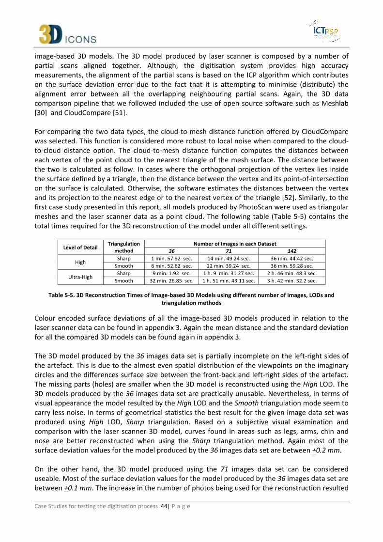
Case Studies for testing the digitisation process 44| P a g e
image-‐based 3D models. The 3D model produced by laser scanner is composed by a number of partial scans aligned together. Although, the digitisation system provides high accuracy measurements, the alignment of the partial scans is based on the ICP algorithm which contributes on the surface deviation error due to the fact that it is attempting to minimise (distribute) the alignment error between all the overlapping neighbouring partial scans. Again, the 3D data comparison pipeline that we followed included the use of open source software such as Meshlab [30] and CloudCompare [51]. For comparing the two data types, the cloud-‐to-‐mesh distance function offered by CloudCompare was selected. This function is considered more robust to local noise when compared to the cloud-‐to-‐cloud distance option. The cloud-‐to-‐mesh distance function computes the distances between each vertex of the point cloud to the nearest triangle of the mesh surface. The distance between the two is calculated as follow. In cases where the orthogonal projection of the vertex lies inside the surface defined by a triangle, then the distance between the vertex and its point-‐of-‐intersection on the surface is calculated. Otherwise, the software estimates the distances between the vertex and its projection to the nearest edge or to the nearest vertex of the triangle [52]. Similarly, to the first case study presented in this report, all models produced by PhotoScan were used as triangular meshes and the laser scanner data as a point cloud. The following table (Table 5-‐5) contains the total times required for the 3D reconstruction of the model under all different settings.
Level of Detail Triangulation
method Number of Images in each Dataset
36 71 142
High Sharp 1 min. 57.92 sec. 14 min. 49.24 sec. 36 min. 44.42 sec. Smooth 6 min. 52.62 sec. 22 min. 39.24 sec. 36 min. 59.28 sec.
Ultra-‐High Sharp 9 min. 1.92 sec. 1 h. 9 min. 31.27 sec. 2 h. 46 min. 48.3 sec. Smooth 32 min. 26.85 sec. 1 h. 51 min. 43.11 sec. 3 h. 42 min. 32.2 sec.
Table 5-‐5. 3D Reconstruction Times of Image-‐based 3D Models using different number of images, LODs and triangulation methods
Colour encoded surface deviations of all the image-‐based 3D models produced in relation to the laser scanner data can be found in appendix 3. Again the mean distance and the standard deviation for all the compared 3D models can be found again in appendix 3. The 3D model produced by the 36 images data set is partially incomplete on the left-‐right sides of the artefact. This is due to the almost even spatial distribution of the viewpoints on the imaginary circles and the differences surface size between the front-‐back and left-‐right sides of the artefact. The missing parts (holes) are smaller when the 3D model is reconstructed using the High LOD. The 3D models produced by the 36 images data set are practically unusable. Nevertheless, in terms of visual appearance the model resulted by the High LOD and the Smooth triangulation mode seem to carry less noise. In terms of geometrical statistics the best result for the given image data set was produced using High LOD, Sharp triangulation. Based on a subjective visual examination and comparison with the laser scanner 3D model, curves found in areas such as legs, arms, chin and nose are better reconstructed when using the Sharp triangulation method. Again most of the surface deviation values for the model produced by the 36 images data set are between +0.2 mm. On the other hand, the 3D model produced using the 71 images data set can be considered useable. Most of the surface deviation values for the model produced by the 36 images data set are between +0.1 mm. The increase in the number of photos being used for the reconstruction resulted
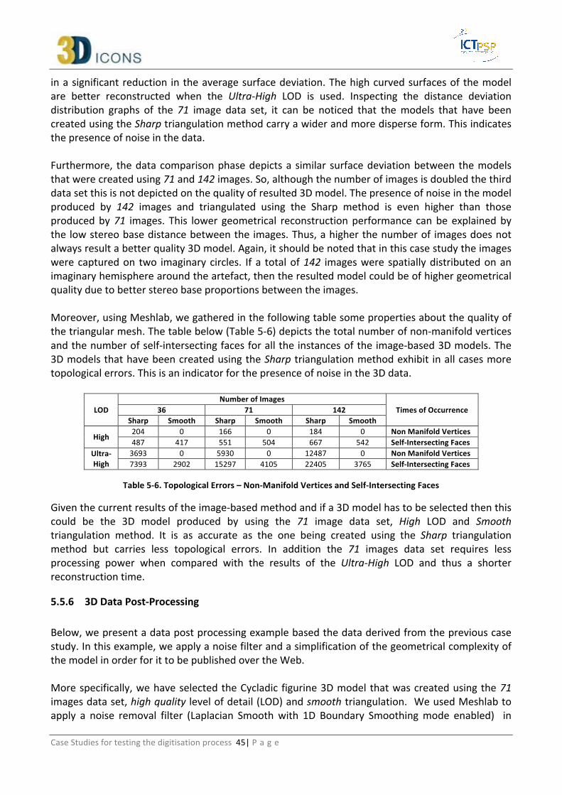
Case Studies for testing the digitisation process 45| P a g e
in a significant reduction in the average surface deviation. The high curved surfaces of the model are better reconstructed when the Ultra-‐High LOD is used. Inspecting the distance deviation distribution graphs of the 71 image data set, it can be noticed that the models that have been created using the Sharp triangulation method carry a wider and more disperse form. This indicates the presence of noise in the data. Furthermore, the data comparison phase depicts a similar surface deviation between the models that were created using 71 and 142 images. So, although the number of images is doubled the third data set this is not depicted on the quality of resulted 3D model. The presence of noise in the model produced by 142 images and triangulated using the Sharp method is even higher than those produced by 71 images. This lower geometrical reconstruction performance can be explained by the low stereo base distance between the images. Thus, a higher the number of images does not always result a better quality 3D model. Again, it should be noted that in this case study the images were captured on two imaginary circles. If a total of 142 images were spatially distributed on an imaginary hemisphere around the artefact, then the resulted model could be of higher geometrical quality due to better stereo base proportions between the images. Moreover, using Meshlab, we gathered in the following table some properties about the quality of the triangular mesh. The table below (Table 5-‐6) depicts the total number of non-‐manifold vertices and the number of self-‐intersecting faces for all the instances of the image-‐based 3D models. The 3D models that have been created using the Sharp triangulation method exhibit in all cases more topological errors. This is an indicator for the presence of noise in the 3D data.
LOD Number of Images
Times of Occurrence 36 71 142 Sharp Smooth Sharp Smooth Sharp Smooth
High 204 0 166 0 184 0 Non Manifold Vertices 487 417 551 504 667 542 Self-‐Intersecting Faces
Ultra-‐High
3693 0 5930 0 12487 0 Non Manifold Vertices 7393 2902 15297 4105 22405 3765 Self-‐Intersecting Faces
Table 5-‐6. Topological Errors – Non-‐Manifold Vertices and Self-‐Intersecting Faces
Given the current results of the image-‐based method and if a 3D model has to be selected then this could be the 3D model produced by using the 71 image data set, High LOD and Smooth triangulation method. It is as accurate as the one being created using the Sharp triangulation method but carries less topological errors. In addition the 71 images data set requires less processing power when compared with the results of the Ultra-‐High LOD and thus a shorter reconstruction time.
3D Data Post-‐Processing 5.5.6 Below, we present a data post processing example based the data derived from the previous case study. In this example, we apply a noise filter and a simplification of the geometrical complexity of the model in order for it to be published over the Web. More specifically, we have selected the Cycladic figurine 3D model that was created using the 71 images data set, high quality level of detail (LOD) and smooth triangulation. We used Meshlab to apply a noise removal filter (Laplacian Smooth with 1D Boundary Smoothing mode enabled) in

Case Studies for testing the digitisation process 46| P a g e
order to reduce the high frequency surface deviations that the image-‐based 3D reconstruction technique produced. Then, we continued with reducing the total number of polygons using again the quadric edge collapse decimation function. The resulted 3D mesh is composed by a total of 81,212 polygons (2.5% of the initial data). The smooth surfaces and the low complexity morphological features are the main reasons for being able to reduce to this extend the polygons of the raw 3D reconstructed mesh while keeping it so close in terms of surface deviation to the laser scanner’s data. More specifically, we compared the produced model against the data produced by the laser scanner (Case Study 5) and we find out that the mean average surface deviation is 28.03μm (Before processing the mean average was 19μm) and the standard deviation (σ) 75.38μm (Before processing the standard deviation was 75μm.). These are values that although they are higher than the unprocessed mesh are still indicating a useable and of acceptable for several applications quality result.

Case Studies for testing the digitisation process 47| P a g e
Processed 3D Mesh 81,212 Triangles 40,608 Vertices 2.5MB (PLY format) Raw 3D Reconstructed Mesh 3,248,488 Triangles 1,624,246 Vertices 61.7MB (PLY format)
Figure 5-‐18. Comparing Raw and Processed 3D Meshes

Case Studies for testing the digitisation process 48| P a g e
Metadata Creation 5.5.7 This section will be completed after the schema for the 3D-‐ICONS is finalized and tested in WP.6.1 and WP 6.2.
3D Data Formats for Publication 5.5.8 This section will be completed after the 3D-‐ICONS deliverable in WP 5.1 is finalised.
Conclusions 5.5.9 This case study attempts to question the application of an image-‐based reconstruction methodology in terms of applicability and 3D data quality on a small artefact. It is obvious that the current Cycladic figurine can be captured in high detail with both laser scanners and structured light systems. The model produced by the 3D laser scanner is of higher quality than all the image-‐based 3D reconstructions and this can be easily understood even with subjective methods (e.g. visual comparison of the different data in terms of geometrical details and lack of noise). The duration of the digitisation procedure using the 3D laser scanner (or a structured light 3D scanner) involves data processing procedures such as cleaning unneeded data and alignment of the partial scans that might require more experienced personnel. On the other hand, the specific image-‐based approach requires the manual generation of masks around the object in order to improve the quality of the reconstructed edges and also to reduce the duration of the reconstruction procedure. The exploitation of an image-‐based 3D reconstruction approach does not involve 3D data processing procedures like a 3D laser scanning or structure-‐light methodology. Nevertheless, a successful photoshooting session involves properties that demand an accurate set up (e.g. camera focus-‐focal length-‐aperture, lighting conditions). Moreover, the texture maps produced by an image-‐based method can be of any7 resolution as practically any camera model can be used. This high resolution images can also be manually mapped on the 3D model produced by a colourless 3D laser scanner but an issue of accurate alignment between geometry and colour can be raised. In addition, a 3D model produced by an image-‐based method can certainly be used in applications where high geometrical details are not a prerequisite. A smooth model of low-‐geometrical complexity accompanied with a high quality image texture map can efficiently be used for dissemination and visualisation purposes over the Web or in other digital mediums such as serious games, multimedia applications, virtual museums, etc. It should also be mentioned that the current case study was based on a challenging artefact. This is due to its surface properties (e.g. lack of strong features, low frequency of colour changes, almost white surface). Nevertheless, the subjective and objective comparison tests resulted that the produced data can be of some use. In addition, both laser scanning and image-‐based methodologies are found to have difficulties when
7 The limitations of current graphics cards and the 3D reconstruction software should be taken under consideration as the upper limit in terms of texture map image resolutions.

Case Studies for testing the digitisation process 49| P a g e
digitising objects with high reflectance surfaces (e.g. of metal surfaces) and transparency (e.g. glass). Generally, in cases where the digitisation system (e.g. laser scanner, structured light) is not a portable system and the artefact cannot be moved in the premises where the digitisation equipment is installed then image-‐based methodologies can be considered as an efficient solution that can provide data that are acceptable for a specific range of applications. Again, the duration and the difficulty of performing both a laser scanning session and a manually implemented photoshooting session are affected by the morphological complexity of the actual artefact (e.g. hollow surfaces, complex appendages, etc.). The total number of partial scans or the total number of images being captured is related to the artefact being digitised. The higher the number of partial scans the higher the duration of the data cleaning and partial scan alignment procedures. Comparing the two methods in terms of time efficiency, the image-‐based method involves a number of fully automated procedures related to the production of a complete 3D model. Furthermore, it should also be noted that for this specific case study the 3D laser scanner that was used is based on a CMM and thus cannot be easily8 transfer to other premises. Hence, the artefact needs always to be brought in the premises where the scanner is installed. This is mentioned only to raise such an important issue as in many cases due to museum regulations or collection institutes limitations this is not possible.
8 A transfer would require a complete disassembly of the system and a new calibration.

Case Studies for testing the digitisation process 50| P a g e
6 Conclusions
Nowadays, 3D digitisation can be performed by a number of different methodologies. These methodologies are offered as commercial or experimental systems. Each methodology is based on different principles and hence aimed for specific types of projects. Currently, there is no single digitisation solution that can be considered as a panacea. Nevertheless, they all share an important property. That is that the duration of the data collection phase is always shorter than the subsequent data post-‐processing phase. The selection of a 3D acquisition method is an important step when designing a digitisation plan. After all, the digitisation plan is greatly correlated by the requirements (e.g. purpose of 3D digitisation, final use of 3D models) and the properties (e.g. budget, duration, available personnel) of a digitisation project. In this report, we have presented a number of case studies that encompass the 3D digitisation of objects derived from the cultural heritage domain based on different methodologies. The case studies cover different types of probable projects such as movable artefacts, unmovable artefacts and the interior and exterior of monuments. Each case study can provide important information for the partners of the project in order to take important decisions related to the design of their own digitisation plans.

Case Studies for testing the digitisation process 51| P a g e
7 References
[1] F. Bellocchio, S. Ferrari, Depth Map and 3D Imaging Applications, 2012, ISBN13 9781613503263. [2] G. Sansoni, M. Trebeschi, F. Docchio, State-‐of-‐The-‐Art and Applications of 3D Imaging Sensors in Industry, Cultural
Heritage, Medicine, and Criminal Investigation, Sensors, Vol. 9, 2009, pp. 568-‐601. [3] A. Koutsoudis, K. Stavroglou, G. Pavlidis, C. Chamzas, 3DSSE -‐ A 3D Scene Search Engine -‐ Exploring 3D Scenes Using
Keywords, Journal of Cultural Heritage, accepted for publication, Aug. 2011. [4] G. Pavlidis, A. Koutsoudis, F. Arnaoutoglou, V. Tsioukas, C. Chamzas, Methods for 3D digitization of Cultural
Heritage, Journal of Cultural Heritage, Volume 8, Issue 1 (2007), pp. 93-‐98. [5] J.A. Beraldin, F. Blais, L. Cournoyer, G. Godin, M. Rioux, Active 3D sensing, Scuola normale superiore pisa, Centro di
Ricerche Informatiche per i Beni Culturali, 2000. [6] M. Rioux, Digital 3-‐D imaging: theory and applications, in procs, of International Symposium on Photonic and
Sensors and Controls for Commercial Applications, Boston, 2650, 1994, pp. 2-‐15. [7] Arius 3D Foundation System, http://www.arius3d.com/a3dscanner.html (last accessed 28-‐1-‐2013). [8] L. Borgeat, G. Godin, P. Massicotte, G. Poirier, F. Blais, J.-‐A. Beraldin, Visualizing and Analyzing the Mona Lisa,
Computer Graphics and Applications, IEEE. Vol 27(6), 12/2007, pp.60-‐68. [9] Konica Minolta Vivid 3D Scanners (discontinued), http://www.konicaminolta.com/instruments/products/3d/non-‐
contact/vivid910/index.html (last accessed 28-‐1-‐2013). [10] NextEngine system (NextEngine, Inc., CA, USA), http://www.nextengine.com [11] Optech Ilris 3D, http://www.optech.ca/prodilris.htm (last accessed 28-‐1-‐2013). [12] Riegl VZ-‐4000, http://www.riegl.com/nc/products/terrestrial-‐scanning/produktdetail/product/scanner/30 (last
accessed 28-‐1-‐2013). [13] Riegl LPM-‐321, http://www.riegl.com/nc/products/terrestrial-‐scanning/produktdetail/product/scanner/2 (last
accessed 28-‐1-‐2013). [14] Faro Focus 3D, http://www.faro.com/focus/us (last accessed 28-‐1-‐2013). [15] J.I. San Jose Alonso, J. Martinez Rubio, J.J. Fernadez Martin, J. Garcia Fernandez, Comparing Time-‐Of-‐Flight and
Phase-‐Shift. The Survey of the Royal Pantheon in the Basilica of San Isidoro (Leon), in procs. of ISPRS Workshop ‘3D-‐ARCH 2011’, March 2-‐4, 2011, Trento, Italy.
[16] Wenguo L., Suping F., Shaujun D., 3D Shape Measurement Based on Structured Light Projection Applying Polynomial Interpolation Technique, International Journal for Light and Electron Optics, in press, available online 18/2/2012.
[17] P. Grussenmeyer, O. A. Khalil, Solutions for Exterior Orientation in Photogrammetry: A Review, The Phogrammetric Record, Vol. 17(100), 2002, pp.615-‐634.
[18] R. Jiang, D. V. Jauregui, K. R. White, Close-‐range photogrammetry applications in bridge measurement: Literature review, Journal of Measurement, Vol. 41 (8), 2008, pp.823-‐834.
[19] F. Dellaert, Structure from motion without correspondence, in: Proceedings of the Computer Vision and Pattern Recognition, Hilton Head, South Carolina, USA, June 13-‐15, 2000, pp. 557-‐564.
[20] D.P. Robertson, R. Cipolla, Structure from motion, Practical Image Processing and Computer Vision, John Willey and Sons Ltd, 2009.
[21] C. Engels, H. Stewénius, D. Nistér, Bundle adjustement rules, in: Proceedings of the Photogrammetric Computer Vision Conference, ISPRS, Bonn, Germany, September 20-‐22, 2006.
[22] N. Snavely, S. M. Seitz, R. Szelinski, Photo tourism: Exploring image collections in 3D, in: Proceedings of SIGGRAPH 2006, Boston Massachusetts, USA, July 30 – August 3, 2006.
[23] N. Snavely, Bundler: Structure from motion for unordered image collections, http://phototour.cs.washington.edu/bundler/#S4 (last accessed 28-‐1-‐2013).
[24] Microsoft Photosynth, http://photosynth.net (last accessed 28-‐1-‐2013).

Case Studies for testing the digitisation process 52| P a g e
[25] C. Wu, S. Agarwal, B. Curless, S. M. Seitz, Multicore bundle adjustment, in: Proceedings of 24th Conference on Computer Vision and Pattern Recognition, June 20-‐25, Colorado Springs, 2011.
[26] C. Wu, VisualSFM: A visual structure from motion system, http://www.cs.washington.edu/homes/ccwu/vsfm (last accessed 28-‐1-‐2013).
[27] Y. Furukawa, J. Ponce, Accurate, dense and robust multi-‐view stereopsis, IEEE Trans. on Pattern Analysis and Machine Intelligence, Vol. 32 (8) 2010 1362-‐1376.
[28] 3D-‐COFORM consortium, http://3dcoform.eu (last accessed 28-‐1-‐2013). [29] Maarten Vergauwen and Luc Van Gool, Web-‐Based 3D Reconstruction Service, Machine Vision Applications, 17, pp.
411-‐426, 2006. [30] Meshlab, http://meshlab.sourceforge.net (last accessed 28-‐1-‐2013). [31] 123D Catch, Autodesk, http://www.123dapp.com/catch (last accessed 28-‐1-‐2013). [32] Hypr3D, Viztu Techonologies, http://www.hypr3d.com (last accessed 28-‐1-‐2013). [33] Insight3D, http://insight3d.sourceforge.net (last accessed 28-‐1-‐2013). [34] PhotoModeler Scanner, http://www.photomodeler.com/products/pm-‐scanner.htm (last accessed 28-‐1-‐2013). [35] PhotoScan Agisoft, http://www.agisoft.ru (last accessed 28-‐1-‐2013). [36] Pix4UAV, http://pix4d.com (last accessed 28-‐1-‐2013). [37] A. Bajard, O. Aubretron, G. Eren, P . Sallamand, F. Truchetet, 3D Digitisation of Metallic Specular Surfaces using
Scanning from Heating Approach, in procs. of SPIE-‐IS&T Electronic Images, Vol. 7864, 2011. [38] H-‐Y Lin, J-‐R Wu, 3D Reconstruction by Combining Shape from Silhouette with Stereo, in procs. of 19th International
Conf. on Pattern Recognition (ICPR 2008), December 8-‐11, 2008, Tampa, Frolida. [39] S.F. El-‐Hakim, J.A. Beraldin, M. Picard, G. Godin, Detailed 3D Reconstruction of Large-‐Scale Heritage Sites with
Integrated Techniques, IEEE Computer Graphics and Applications, March-‐June 2004, pp. 21-‐29. [40] G. Müller, G. H. Bendels, R. Klein, Rapid Synchronous Acquisition of Geometry and Appearance of Cultural Heritage
Artefacts, in procs. of the 6th International Symposium on Virtual Reality, Archaeology and Cultural Heritage (VAST), November 8-‐11, 2005, Pisa, Italy.
[41] M. Holroyd, J. Lawrence, T. ZIckler, A Coaxial Optical Scanner for Synchronous Acquisition of 3D Geometry and Surface Reflectance, Transactions on Graphics, Vo. 29 (4), Article 99, 2010.
[42] C. Schwartz, M. Weinmann, R. Ruiters, R. Klein. Integrated High-‐Quality Acquisition of Geometry and Appearance for Cultural Heritage, in procs. of the International Symposium on Virtual Reality, Archaeology and Cultural Heritage (VAST), October 18-‐21, 2011, Tuscany, Italy.
[43] M. Callieri, R. Scopigno, 3D Scanning, Improving completeness, processing speed and visualisation, Eurographics Italian Section, Winter School 2005, http://vcg.isti.cnr.it/EGIT05/EG_IT%20Terzo%20Convegno_file/pdf/EGIT05_scateni.pdf (last accessed 28-‐1-‐2013).
[44] G. Tsigaras, Kioutouklou Baba Bekctashic Tekke, Regional guide of eastern Macedonia and Thrace, http://www.xanthi.ilsp.gr/cultureportalweb/print.php?article_id=140&lang=en&print_mode=article (last accessed 28-‐1-‐2013).
[45] H.W. Lowry, In the footsteps of the Ottomans: A search for sacred spaces and architectural monuments in northern Greece, Mary Martin Booksellers, Bahçesehir University Publications, 2009.
[46] M.H. Nguyen, B. Wuensche, P. Delmas, C. Lutteroth, 3D models from the black box: Investigatin the current state of image-‐based modeling, in: Proceedings of the 20th International Conference on Computer Graphics, Visualisation and Computer Vision (WSCG 2012), Pilsen, Czech Republic, June 25-‐28, 2012.
[47] Topcon GPT-‐3005N total station, http://www.topcon.com.sg/survey/gpt30.html (last accessed 28-‐1-‐2013). [48] S. M. Seitz, B. Curless, J. Diebel, D. Scharstein, R. Szeliski, Evaluation of Multi-‐View Stereo Reconstruction
Algorithms, in proceedings of IEEE Computer Society Conference on Computer Vision and Pattern Recognition (CVPR ’06), Vol.1 (1), IEEE computer society, June 17-‐22, 2006, Washington, DC, pp. 519-‐528.
[49] D. Scharstein, R. Szeliski, A taxonomy and evaluation of dense two-‐stereo correspondence algorithms, Journal of Computer Vision 47 (2002) 7-‐42.
[50] Meshlab, http://meshlab.sourceforge.net (last accessed 28-‐1-‐2013). [51] CloudCompare, http://www.danielgm.net/cc (last accessed 28-‐1-‐2013).

Case Studies for testing the digitisation process 53| P a g e
[52] D. Eberly, Distance between Point and Triangle in 3D, Geometric Tools LLC, http://www.geometrictools.com/Documentation/DistancePoint3Triangle3.pdf (last accessed 28-‐1-‐2013).
[53] J. P. Dandois, E. C. Ellis, Remote Sensing of Vegetation Structure Using Computer Vision, Remote Sensing, Vol. 2(4), 2010, pp.1157-‐1176.
[54] Ecosynth Team Blog, http://ecotope.org/ecosynth/blog/post/2011/12/17/TLS-‐scanning-‐at-‐UMBC.aspx (last accessed 28-‐1-‐2013).
[55] G. Gabriele, G. Danilo, B. Marco, The employment of terrestrial laser scanner in cultural heritage conservation: the case study of Vallinotto Chapel in Carignano-‐Italy, Appl Geomat, Vol 2, 2010, pp. 59-‐63.
[56] D. Papakostas, Digitisation of Rotunda using a Laser Scanner, Undergraduate Thesis, Aristotle University of Thessaloniki, Department of Topography, March 2011, http://invenio.lib.auth.gr/record/126348/files/GRI-‐2011-‐6551.pdf (last accessed 28-‐1-‐2013).
[57] A. Vianello, Which was the role of Cycladic marble figurines in funerary rituals?, http://www.bronzeage.org.uk/publications/4.pdf (last accessed 28-‐1-‐2013).
[58] Archaeological Receipts Fund, Female Figure, http://www.tap.gr/tapadb/index.php/en/component/jshopping/product/view/1/7 (last accessed 28-‐1-‐2013).
[59] N. Papadimitriou, The use and meaning of Cycladic figurines, Special Topic on Cycladic Culture, Museum of Cycladic Art, Nicholas and Dolly Goulandris Foundation, http://www.cycladic.gr/frontoffice/portal.asp?cpage=resource&cresrc=126&cnode=40&clang=1 (last accessed 28-‐1-‐2013).
[60] Arius 3D Foundation 100, http://www.arius3d.com/a3dscanner.html (last accessed 28-‐1-‐2013). [61] M. Zwicker, H. Pfister, J. Baar, M. Gross, Surface Splatting, in procs. of SIGGRAPH 2001, 12-‐17 August 2001, Los
Angeles, CA, USA, pp.371-‐378. [62] J. Krivanek, Representin and Rendering Surfaces with Points, Postgraduate Study Report, Department of Computer
Science and Engineering, Czech Technical University, February 2003, http://cgg.mff.cuni.cz/~jaroslav/papers/minimum/minimum.pdf (last accessed 28-‐1-‐2013).
[63] L. S. Kalos, T. Umenhoffer, Displacement Mapping on the GPU – State of the Art, Computer Graphics Forum, Volume 27, Number 6, 2008, pp. 1567-‐1592.
[64] V. Krishnamurthy, M. Levoy, Fitting Smooth Surfaces to Dense Polygon Meshes, in procs. of SIGGRAPH ’96, New Orleans, Louisiana, USA, http://graphics.stanford.edu/papers/surfacefitting (last accessed 28-‐1-‐2013).
[65] J. Wang, M. M. Oliveira, A Hole-‐Filling Strategy for Reconstruction of Smooth Surfaces in Range Images, in procs. of the XVI Brazilian Symposium on Computer Graphics and Image Processing, São Carlos, SP. October 12-‐15, 2003, pp. 11-‐18.
[66] P. Cignoni, C. Montani, R. Scopigno, A Comparison of Mesh Simplification Algorithms, Computers & Graphics Vol.22, No.1 (1998). pp. 37-‐54.
[67] H. Hoppe. Progressive Meshes, in procs. of SIGGRAPH '96 Conference (1996), pp. 99-‐108. [68] W. J. Schroeder, J. A. Zarge, W. E. Lorensen. Decimation of Triangle Meshes, in procs. of SIGGRAPH 92 Conference
(1992), pp. 65-‐70. [69] G. Gahm, Mesh Decimation, http://www.gustavgahm.com/wp-‐
content/upload/moa/Gustav_Gahm_Mesh_Decimation.pdf (last accessed 28-‐1-‐2013). [70] 3D COAT – Retopology Tool, http://3d-‐coat.com/download (last accessed 29-‐1-‐2013). [71] Blender – 3D Modelling Tool, http://www.blender.org (last accessed 29-‐1-‐2013). [72] Zbrush http://www.pixologic.com (last accessed 29-‐1-‐2013). [73] GSculpt, http://gsculpt.sourceforge.net (last accessed 29-‐1-‐2013). [74] GPU Gems 2, Per-‐Pixel Displacement Mapping with Distance Functions, Chapter 8, Nvidia, ISBN 0-‐321-‐33559-‐
72005, pp. 123-‐136. [75] xNormal, http://www.xnormal.net (last accessed 28-‐1-‐2013). [76] J.X. Chen, Guide to Graphics Software Tools, Springer-‐Verlag London Limited 2009, 1-‐4, DOI: 10.1007/978-‐1-‐84800-‐
901-‐1_18. [77] Deep Exploration, http://www.righthemisphere.com/products/dexp/de_std.html (last accessed 28-‐1-‐2013).

Case Studies for testing the digitisation process 54| P a g e
[78] VRML, http://en.wikipedia.org/wiki/VRML (last accessed 28-‐1-‐2013). [79] Web 3D consortium, http://www.web3d.org/realtime-‐3d/x3d-‐vrml/html-‐3d (last accessed 28-‐1-‐2013). [80] J. Behr,Y. Jung,A Scalable Architecture for the HTML5/X3D Integration Model X3DOM, In proc. Of 37th SIGRAPH
2010, July 27-‐29, Los Angeles, USA., http://www.web3d.org/event/s2010/HTML5-‐X3D-‐Integration.pdf (last accessed 28-‐1-‐2013).
[81] BS Contact – Bitmanagement, http://www.bitmanagement.com (last accessed 28-‐1-‐2013). [82] The Gzip GNU compression utility, http://www.gzip.org (last accessed 28-‐1-‐2013). [83] Standard ECMA-‐363 Universal 3D File Format, http://www.ecma-‐international.org/publications/standards/Ecma-‐
363.htm (last accessed 28-‐1-‐2013). [84] PRC Format Specification,
http://livedocs.adobe.com/acrobat_sdk/9/Acrobat9_HTMLHelp/API_References/PRCReference/PRC_Format_Specification/index.html (last accessed 28-‐1-‐2012).
[85] A. Koutsoudis, WebGL 3DGallery, http://www.ipet.gr/~akoutsou/x3d/demo (last accessed 28-‐1-‐2012). [86] O3D, http://code.google.com/p/o3d (last accessed 28-‐1-‐2012). [87] Unity3D, http://unity3d.com (last accessed 28-‐1-‐2012). [88] OpenSpace3D, http://www.openspace3d.com (last accessed 28-‐1-‐2012). [89] TurnTool, http://www.turntool.com (last accessed 28-‐1-‐2012).

Case Studies for testing the digitisation process 55| P a g e
8 Appendices
8.1 Appendix 1 – Case Study 1: Data Accuracy Comparison Figure 8-‐1 illustrates colour encoded surface deviations of the monument’s exterior surfaces. Each surface deviation depiction is followed by a graph showing the deviation distance frequency of occurrence along with the mean distance and the standard deviation (σ) of the scans. An increase in the mean distance and the standard deviation can be seen in the part of roof tile (Figure 8-‐1, Scan Num. 3, Scan Num. 7). This is an indication of the inability of SFM-‐DMVR methods to reconstruct surfaces of low features. The low frequency of colour alternations on the roof tiles in conjunction with the bad lighting in the hollow areas between every alternate roof tile row composes a challenging, for SFM-‐DMVR methods, surface. In addition, Table 8-‐1 shows all the mean distances and standard deviations of the range scans that have been compared against the mesh produced by PhotoScan. It should be noted that all comparisons resulted in Gaussian like distributions. As each range scan covered an area of different size, the total number of vertices that compose each scan was used as a contribution weight to the average mean distance and standard deviation. As shown in Table 8-‐1, the total weighted average mean distance between the two data types is 1.8 mm and the total weighted standard deviation 14.3 mm.
Scan Num. 1

Case Studies for testing the digitisation process 56| P a g e
Scan Num.2
Scan Num. 3
Scan Num. 4

Case Studies for testing the digitisation process 57| P a g e
Scan Num. 5
Scan Num. 6
Scan Num. 7
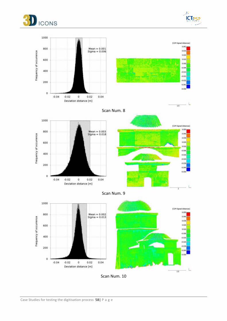
Case Studies for testing the digitisation process 58| P a g e
Scan Num. 8
Scan Num. 9
Scan Num. 10

Case Studies for testing the digitisation process 59| P a g e
Scan Num. 11
Figure 8-‐1 Colour encoded surface deviation of different parts of the monument and distance deviation distribution graphs
Scan No. Mean Distance Standard Deviation (σ) 1 0.001 0.008 2 0.000 0.005 3 0.003 0.017 4 0.001 0.010 5 0.001 0.010 6 0.003 0.020 7 0.004 0.012 8 0.001 0.006 9 0.003 0.018 10 0.002 0.013 11 0.002 0.014
Weighted Averages (in meters) 0.002 0.014
Table 8-‐1 Individual mean distances and standard deviations of each single-‐view range scan compared to the image-‐based mesh.

Case Studies for testing the digitisation process 60| P a g e
Figure 8-‐2 Line segments defined by feature points on the surface of the monument used for data accuracy
verification
Line Segment Distance Using Total Station Data
Distance Using Range Scan Data
Distance Using SFM-‐DMVR Data
Normalized error for RS (%)
Normalized error for SFM-‐DMVR (%)
AB 7.580 7.592 7.601 0.2 0.3
CD 3.745 3.747 3.751 0.1 0.2
EF 3.184 3.186 3.189 0.1 0.2
GH 0.473 0.469 0.467 0.8 1.3
GI 2.313 2.313 2.311 0.0 0.1
JK 2.958 2.973 2.972 0.5 0.5
LM 1.876 1.868 1.881 0.4 0.3
NQ 3.491 3.496 3.486 0.1 0.1
ON 4.877 4.874 4.871 0.1 0.1
PR 2.661 2.672 2.665 0.4 0.2
SU 3.184 3.184 3.172 0.0 0.4
TS 4.713 4.703 4.694 0.2 0.4 Average 0.24 0.32
Table 8-‐2 Comparison of Euclidean distances between feature points on the different types of 3D Data (in meters)
On the other hand, we attempted to verify a set of empirical measurements that have been previously performed on the surface of the monument between fine details on the surface of the monument (Figure 8-‐2). These distances varied between 7cm and 30cm. Again, using Meshlab, we performed the same distance measurements on the SFM-‐DMVR mesh. The results were found to be acceptable for a project that aims in visualising 3D models of monuments over the Web.

Case Studies for testing the digitisation process 61| P a g e
Line Segment Distance on Real Monument Distance on SFM-‐DMVR data Normalized error (%)
VW 0.233 0.233 0.00
XY 0.290 0.288 0.69
''ED 0.283 0.283 0.00
'ZA 0.181 0.179 1.10
''CB 0.714 0.715 0.14
''GF 1.160 1.160 0.00
Average 0.16
Table 8-‐3 Comparison of Euclidean distances between empirical measurements and manual measurements on the SFM-‐DMVR data (in meters)
The previous experiments contributed on verifying that the SFM-‐DMVR model does not contain proportional errors.

Case Studies for testing the digitisation process 62| P a g e
8.2 Appendix 2 – Case Study 2: Image scale and Ground Sample Distance (GSD) The degree of detail that can be seen in a photograph is mainly dependent on the resolution of the camera/lens system and on the photographic scale. Digital cameras have discrete finite elements on the sensor surface called pixels. Pixels are usually square elements whose side length is in the order of some microns. Objects in the real world are recorded in a discretized way on digital camera sensors (CCD or CMOS) and the level of detail (LOD) of this discretization is proportional to the distance between the camera and the object. The scale M is the ratio between the principal distance c (approximately the focal length) of the lens and the distance h of the camera from the object (Fig. 8.1):
M=c/h
Basically, the scale M is the number of times a real object is enlarged on the image sensor. The level of detail visible on the image is directly proportional to the scale M, so an high scale number correspond to a high level of detail. Given a specific camera-‐lens system, the closer the distance h, the higher the level of detail visible on the image (Figure 8-‐3-‐ left). Given a certain camera at a fixed distance from an object, the level of detail can be increased/decreased using a longer/shorter focal length c (Figure 8-‐3-‐ right). In latter case, the use of a long focal lengths requires a larger number of images in order to cover the entire object.
Figure 8-‐3. Example of possible scales in imaging acquisition
Given a specific scale number, at a linear measurement x’ on the sensor (“image space”) corresponds a linear measurement X in the real world (“object space”). If the segment x’ is as small as the pixel size (the side of a pixel considered a square) the segment X in the object space is called Ground Sampling Distance (GSD) or footprint (Figure 8-‐4). The maximum accuracy achievable can be said to be roughly within two times the GSD for manual measurements. In case of automated measurements, accuracy up to 1/10 of a pixel can be achieved. Actually, the accuracy is different in the three dimensions and is generally worse for the depth direction.

Case Studies for testing the digitisation process 63| P a g e
Figure 8-‐4. Image scale and relation with linear measurements in image and object space
The limit distance Hmax is the maximum relative distance between the camera and the object and is defined as follows:
csizepix
GSDMcH ⋅==
_max
Where pix_size is the dimension of the pixel element of the employed camera (length of the side of the sensor’s pixel considered as squared element). Assuming a digital camera ca 6.5 micron pixel size and a 20 mm lens, if we need to have a GSD of 3 mm, the Hmax should be around 9 meters. Therefore the maximum distance (hmax) from the object allowed during the image acquisition phase is ca 9 m. This value is of course an ideal value that can be considered valid only with perfect lenses, in absence of blur effects and when the entire surface of the object is planar and parallel to the image plane. If we consider for example that the surface of the object has a tilt angle of 45 degrees respect to the view angle the maximum distance should
be reduced for a factor 7.021
≈ . Therefore in practical cases, depending on the project
tolerances, it might be necessary to reduce the limit distance from the object even to the half of the ideal one. The GSD is an important parameter for the photographic acquisition because tells how much space around the object should be free of obstructions/obstacles to record it properly. It is a rule of thumb that each point of the object should be visible in at least three images (redundancy) but is also important to have a good distance among cameras (baselines) to assure good intersection angles. Photogrammetry is based on the triangulation measurement principle for reconstructing the imaged object in 3D. Thus at least two views of a same 3D point taken from different positions must be available. Furthermore the point to be measured and the two camera positions must be not aligned i.e. must form a triangle. The closer the intersecting angle among the optical rays to 90 degrees, the better the intersection. A classical image acquisition’s schema for a simple object is depicted in Figure 8-‐5. This schema of course holds only when there are no objects interfering with the field of view or the camera

Case Studies for testing the digitisation process 64| P a g e
position itself. In real cases there are obstructions, light changes and other restrictions that impose changes of the planned schema.
Figure 8-‐5. Typical image acquisition schema for a simple fragment. It is important to find a good compromise
between image baseline and number of images in order to achieve a good reconstruction accuracy and, if necessary, automated processing.

Case Studies for testing the digitisation process 65| P a g e
8.3 Appendix 3 – Case Study 5: Data Accuracy Comparison The following figure (Figure 8-‐6) illustrates colour encoded surface deviations of all the image-‐based 3D models produced in relation to the laser scanner data. Each surface deviation depiction is followed by a graph showing the deviation distance frequency of occurrence along with the mean distance and the standard deviation (σ) between the laser scanner model and each of the image-‐based 3D models. Then, a thumbnail of each image-‐based 3D model is also illustrated for a subjective evaluation of the result. Table 8-‐4 gathers the mean distance and the standard deviation (σ) for all the compared 3D models.
36 Images Data Set – High LOD – Sharp Triangulation
36 Images Data Set – High LOD – Smooth Triangulation
36 Images Data Set – Ultra High LOD – Sharp Triangulation

Case Studies for testing the digitisation process 66| P a g e
36 Images Data Set – Ultra High LOD – Smooth Triangulation
71 Images Data Set – High LOD – Sharp Triangulation
71 Images Data Set – High LOD – Smooth Triangulation
71 Images Data Set – Ultra High LOD – Sharp Triangulation

Case Studies for testing the digitisation process 67| P a g e
71 Images Data Set – Ultra High LOD – Smooth Triangulation
142 Images Data Set – High LOD – Sharp Triangulation
142 Images Data Set – High LOD – Smooth Triangulation
142 Images Data Set – Ultra High LOD –Sharp Triangulation
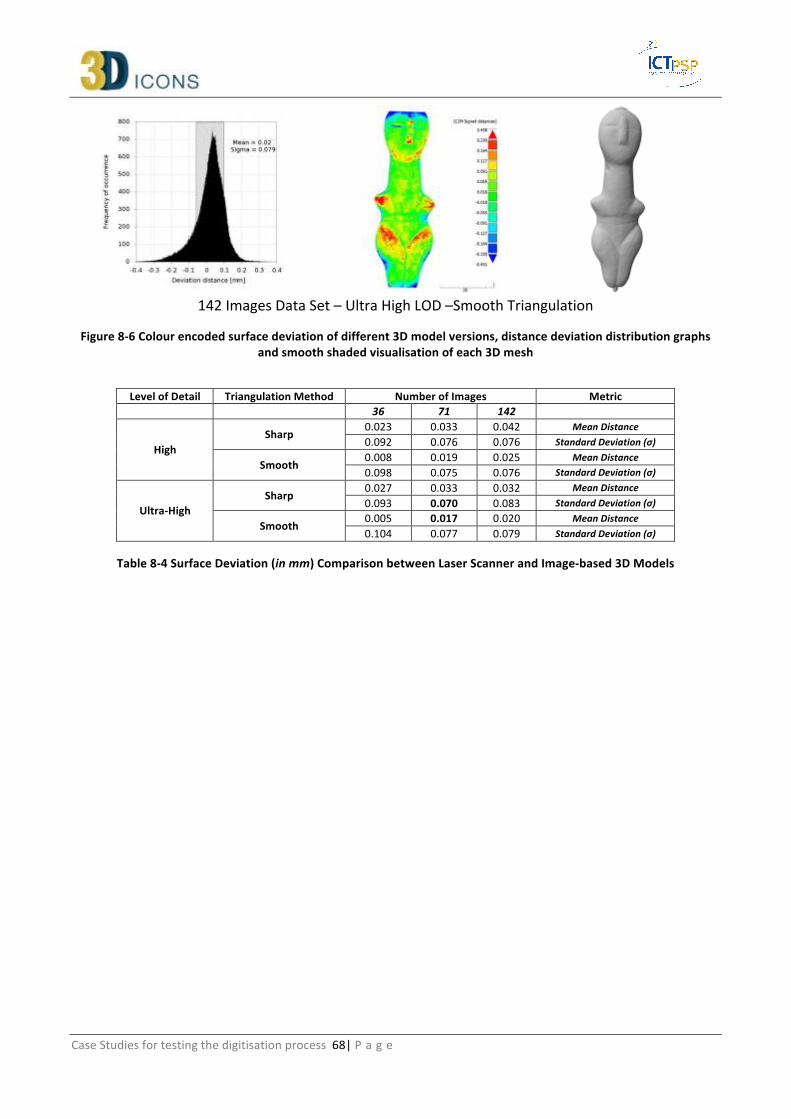
Case Studies for testing the digitisation process 68| P a g e
142 Images Data Set – Ultra High LOD –Smooth Triangulation
Figure 8-‐6 Colour encoded surface deviation of different 3D model versions, distance deviation distribution graphs and smooth shaded visualisation of each 3D mesh
Level of Detail Triangulation Method Number of Images Metric 36 71 142
High Sharp
0.023 0.033 0.042 Mean Distance 0.092 0.076 0.076 Standard Deviation (σ)
Smooth 0.008 0.019 0.025 Mean Distance 0.098 0.075 0.076 Standard Deviation (σ)
Ultra-‐High Sharp
0.027 0.033 0.032 Mean Distance 0.093 0.070 0.083 Standard Deviation (σ)
Smooth 0.005 0.017 0.020 Mean Distance 0.104 0.077 0.079 Standard Deviation (σ)
Table 8-‐4 Surface Deviation (in mm) Comparison between Laser Scanner and Image-‐based 3D Models