Deliverable D 3.3 S2R innovation first periodic assessment

Modelling and strategies for the assessment and Optimisation of Energy

Usage aspects of rail innovation

Deliverable D 3.3 S2R innovation first periodic assessment

Reviewed: (yes/no)

Project acronym: OPEUS

Starting date: 01/11/2016

Duration (in months): 30

Call (part) identifier: H2020-S2R-OC-CCA-2015-02

Grant agreement no: 730827

Due date of deliverable: Month 24

Actual re-submission date: 07/07/2020

Responsible/Author: Lukas Pröhl – University of Rostock

Dissemination level: PU

Status: Final

Ref. Ares(2020)3582933 - 07/07/2020

G A 7 3 0 8 2 7 P a g e 2 | 52

Document history

Revision Date Description

Part 1 - V00 07.02.2018 Document initiated.

Part 1 - V01 03.04.2018 Content updated.

Part 1 - V02 13.04.2018 Content update with battery part.

Part 1 - V03 18.04.2018 Content update and development. Issued to OPEUS consortium for review.

Part 1 - V04 27.04.2018 Partner remarks and feedback. Content update to address feedback.

Part 1 - V05 02.05.2018 Content update to address feedback.

Part 1 - V06 30.05.2018 Content update to address feedback.

Part 2 - V00 04.09.2018 Document initiated.

Part 2 - V01 31.10.2018 Content updated – simulation results updated

Part 2 - V02 15.10.2018 Content update and development. Issued to OPEUS consortium for review.

Part 2 - V03 19.10.2018 Content update according to review feedback for section 9

Part 2 - V04 28.10.2018 Content update according to partners feedback

Part 2 - V05 29.10.2018 Content update – Simulation results for section 9



Final 25.04.2019 Document finalised for submission to S2R.

Final v2 07.07.2020 Originally submitted deliverable Report Part 1 and Part 2 combined and de-duplicated to form cohesive report for re-submission to S2R.

Report contributors

Name Beneficiary Short Name

Details of contribution

L. Pröhl UROS Author

H. Aschemann UROS Author

J Kersten UROS Review

D. Nguyen SAFT Author (Battery simulations, Section 5.2) and review

I. De Keyzer UIC Review

M. Marsilla STAV Review

D. Kuzmina UITP Review

L. Dauby UITP Review

B. Fairbairn UNEW Review

R. Palacin UNEW Review

http://www.inaf.it/it/sedi/sede-centrale-nuova/direzione-scientifica/relazioni-internazionali/nuovo-logo-horizon-2020/view

G A 7 3 0 8 2 7 P a g e 3 | 52

Executive Summary This report ‘DO3.3 - S2R innovation first periodic assessment’ is the first element of a two-part deliverable series comprising DO3.3 and DO3.4, which together provide the periodic assessment of the technical innovations within OPEUS and Shift2Rail. D03.3 focuses on the investigations done within the first stage of the OPEUS project, then builds upon the reported investigations and technical approaches. The main objective is to introduce and provide a periodic overview and analysis for the investigated innovations within the technical OPEUS work packages (WP4, WP5 and WP6) as well as a presentation of the corresponding energy simulation results. Firstly, the theoretical background of the investigated innovation approaches (esp. energy storage system and driving strategy) is described. Secondly, these approaches are included in the simulation structure of the OPEUS-tool (developed within WP2 “Simulation model and tool development”, see [1], [2]). Furthermore, the OPEUS-tool is applied to perform the energy simulations with these implemented approaches. To enable a proper assessment of the technical innovations, the arising simulation results are compared to the baseline scenario simulations that are described in deliverable ‘DO3.2 – Baseline simulation results and assessment’ [3]. Based on these comparisons the potential of the investigated innovations is discussed. The outcomes of this report are expected to support the WP4 and WP6 in order to provide an opportunity to analyse the investigated techniques as well as to determine the focus for further investigations. Additionally, this report serves as an input for WP7, which has the objective to provide a summary as well as a global vison of energy usage in railway applications.


G A 7 3 0 8 2 7 P a g e 4 | 52

Table of Contents Executive Summary ........................................................................................................................... 3

List of Figures ..................................................................................................................................... 5

List of Tables ...................................................................................................................................... 7

List of Symbols ................................................................................................................................... 8

Abbreviations and acronyms ............................................................................................................. 9

1 Background and Objective ........................................................................................................ 10

2 Introduction .............................................................................................................................. 11

3 Summary of the reference scenarios ........................................................................................ 12

4 Operating strategy to optimise in-vehicle energy losses.......................................................... 15

5 Implementation of energy storage systems ............................................................................. 20

5.1 Operating strategy for energy storage systems ............................................................... 20

5.2 Scenario simulations with energy storage systems .......................................................... 23

5.3 Optimized ESS management ............................................................................................. 27

6 Driving strategy improvements ................................................................................................ 35

6.1 Optimisation approach for the energy-optimal driving strategy ..................................... 37

6.2 Simulation results for energy optimised velocity profiles ................................................ 39

6.3 Influence of gradients ....................................................................................................... 43

6.4 DAS outlook to deliverable DO3.3 - part 3 ....................................................................... 50

7 Conclusion ................................................................................................................................. 51

8 References................................................................................................................................. 52


G A 7 3 0 8 2 7 P a g e 5 | 52

List of Figures Figure 1: Possible trajectory modes ................................................................................................ 13

Figure 2: Component efficiency for different loads ........................................................................ 15

Figure 3: Velocity and power profiles at the catenary level for the comparison of the baseline result with the utilisation of partial switch-offs of traction components (Reg160) ................. 16

Figure 4: Details of the velocity and power profiles at the catenary level for the comparison of the baseline result with the utilisation of partial switch-offs of traction components (Reg160) .......................................................................................................................... 17

Figure 5: Energy savings caused by partial switch-offs for the defined drive cycles ...................... 18

Figure 6: Composition of energy savings at the DC link .................................................................. 19

Figure 7: Basic approach for operating strategy for ESS ................................................................. 20

Figure 8: Energy simulation results for varying ESS operating parameters εtrac, εaux and a fixed recuperation parameter εrec (Reg160) ........................................................................... 22

Figure 9: State of charge at the end of the drive cycle for varying ESS operating parameters εtrac, εaux and a fixed recuperation parameter εrec (Reg160) ................................................ 22

Figure 10: Definition of four non-electrified zones with constant vehicle speed: train position in km (blue curve), train speed in km/h (red curve) ................................................................. 24

Figure 11: Electrical power (red curve) and SOC (blue curve) of the ESU-battery .......................... 25

Figure 12: Traction energy (in kWh) calculated at the catenary ..................................................... 26

Figure 13: Recuperated energy (in kWh) to the catenary ............................................................... 26

Figure 14: Charging time (in minutes) of the battery at the end of the course .............................. 27

Figure 15: Velocity trajectory and State-of-Charge for HS250 service ............................................ 29

Figure 16: Power profile at the ESS (balanced SoC) for HS250 service ........................................... 29

Figure 17: Power profile at the catenary for ESS application (balanced SoC) for HS250 service ... 29

Figure 18: Velocity trajectory and State-of-Charge for Reg160 service .......................................... 30

Figure 19: Power profile at the ESS (balanced SoC) for Reg160 service ......................................... 30

Figure 20: Power profile at the catenary for ESS application (balanced SoC) for Reg160 service .. 30

Figure 21: Velocity trajectory and State-of-Charge for Tram service .............................................. 31

Figure 22: Power profile at the ESS (balanced SoC) for Tram service ............................................. 31

Figure 23: Power profile at the catenary for ESS application (balanced SoC) for Tram service ..... 31

Figure 24: Velocity trajectory and State-of-Charge for Metro service ............................................ 32

Figure 25: Power profile at the ESS (balanced SoC) for Metro service ........................................... 32

Figure 26: Power profile at the catenary for ESS application (balanced SoC) for Metro service ... 32

Figure 27: Velocity trajectory and State-of-Charge for Freight Mainline service ........................... 33

Figure 28: Power profile at the ESS (balanced SoC) for Freight service .......................................... 33

Figure 29: Power profile at the catenary for ESS application (balanced SoC) for Freight service .. 33

Figure 30: Possible trajectory modes .............................................................................................. 35


G A 7 3 0 8 2 7 P a g e 6 | 52

Figure 31: Relative energy savings based on the implementation of coasting and the total net energy consumption for both trajectory modes ............................................................ 36

Figure 32: Driving strategy parameters ........................................................................................... 37

Figure 33: Possible driving styles to fulfil the timetable ................................................................. 38

Figure 34: Baseline and energy optimised velocity trajectories for HS300 service ........................ 40

Figure 35: Power profile at the catenary for optimised driving strategy for HS300 service ........... 40

Figure 36: Baseline and energy optimised velocity trajectories for HS250 service ........................ 41

Figure 37: Power profile at the catenary for optimised driving strategy for HS250 service ........... 41

Figure 38: Baseline and energy optimised velocity trajectories for Freight Mainline service ........ 42

Figure 39: Power profile at the catenary for optimised driving strategy for Freight Mainline ....... 42

Figure 40: Velocity trajectories for HS300 track profile with and without gradient ....................... 45

Figure 41: Power profile at the catenary for various gradient scenarios for HS300 service .......... 45

Figure 42: Velocity trajectories for Reg140 track profile with and without gradient ..................... 46

Figure 43: Power profile at the catenary for various gradient scenarios for Reg140 service ......... 46

Figure 44: Power profile at the catenary for various gradient scenarios for Reg140 service - extract ......................................................................................................................................... 46

Figure 45: Velocity trajectories for Metro track profile with and without gradient ....................... 47

Figure 46: Power profile at the catenary for various gradient scenarios for Metro service ........... 47

Figure 47: Power profile at the catenary for various gradient scenarios Metro service - extract .. 47

Figure 48: Velocity trajectories for Tram track profile with and without gradient ......................... 48

Figure 49: Power profile at the catenary for various gradient scenarios for Tram service ............ 48

Figure 50: Velocity trajectories for Freight Mainline track profile with and without gradient ...... 49

Figure 51: Power profile at the catenary for various gradient scenarios for Freight Mainline service ......................................................................................................................................... 49


G A 7 3 0 8 2 7 P a g e 7 | 52

List of Tables Table 1: Boundary conditions for the baseline scenario simulation (see [3]) ................................. 13

Table 2: Total energy consumption of reference scenario simulations .......................................... 14

Table 3: Considered scenarios with the presence of ESU-battery .................................................. 24

Table 4: ESS operating parameters.................................................................................................. 28

Table 5: Simulation results for ESS application (balanced SoC) for HS250 service ......................... 29

Table 6: Simulation results for ESS application (balanced SoC) for Reg160 service ....................... 30

Table 7: Simulation results for ESS application (balanced SoC) for Tram service ........................... 31

Table 8: Simulation results for ESS application (balanced SoC) for Metro service ......................... 32

Table 9: Simulation results for ESS application (balanced SoC) for Freight Mainline service ......... 33

Table 10: Power peak reduction during recuperation due to ESS application ............................... 34

Table 11: Simulation results for energy optimised velocity trajectory for HS300 service .............. 40

Table 12: Simulation results for energy optimised velocity trajectory for HS250 service .............. 41

Table 13: Simulation results for energy optimised velocity trajectory for Freight Mainline service ......................................................................................................................................... 42

Table 14: Simulation results for gradient influence for HS300 service ........................................... 45

Table 15: Simulation results for gradient influence for Reg140 service ......................................... 46

Table 16: Simulation results for gradient influence for Metro service ........................................... 47

Table 17: Simulation results for gradient influence for Tram service ............................................. 48

Table 18: Simulation results for gradient influence for Freight Mainline ....................................... 49


G A 7 3 0 8 2 7 P a g e 8 | 52

List of Symbols Symbol Description

𝛼𝑠, 𝛼𝑡 Weight factors for distance and time

𝑏𝑐 Driving style parameter for coasting application

𝑐𝑜𝑛𝑠, 𝑐𝑜𝑛𝑠 Constrains for distance and time

𝐸𝑐𝑜𝑛𝑠 Consumed energy at the catenary

𝐸𝑛𝑒𝑡 Total net energy budget at the catenary

𝐸𝑟𝑒𝑐 Recuperated energy at the catenary

𝐸𝑡𝑜𝑡𝑎𝑙 Total energy consumption

∆𝐸𝐸𝑆𝑆 Energy deviation at the ESS

𝜀𝑟𝑒𝑐, 𝜀𝑡𝑟𝑎𝑐, 𝜀𝑎𝑢𝑥 Operating parameters for the ESS

𝐽𝐷𝑆 Coast function for driving style

�̅�𝑚𝑜𝑡 Number of applied motors

𝑛𝑚𝑜𝑡 Total number of motors per train

�̅�𝑖𝑛𝑣 Number of applied motor inverters

𝑛𝑖𝑛𝑣 Total number of motor inverters per train

𝑃𝑏𝑎𝑡 Battery power

𝑃𝑐𝑎𝑡,𝑟𝑒𝑐 Recuperated power to the catenary

𝑃𝑐𝑎𝑡,𝑡𝑟𝑎𝑐 Traction power supplied by the catenary

𝑃𝐷𝐶 Power request at the DC intermediate circuit

𝑃𝐷𝐶,𝑎𝑢𝑥 Auxiliary power at the DC intermediate circuit

𝑃𝐸𝑆𝑆,𝑎𝑢𝑥 Auxiliary power supplied by the ESS

𝑃𝐸𝑆𝑆.𝑟𝑒𝑐 Recuperated power to the ESS

𝑃𝐸𝑆𝑆,𝑡𝑟𝑎𝑐 Traction power supplied by the ESS

𝑃𝑡𝑟𝑎𝑐 Traction power

𝑃𝑡𝑜𝑡𝑎𝑙 Total power request per component

𝑃𝑚𝑎𝑥,𝑚𝑜𝑡 / 𝑃𝑚𝑎𝑥,𝑖𝑛𝑣 Maximum power per motor / motor inverter

𝑝𝑣𝑎 Driving style parameter for velocity restriction

𝑆𝑂𝐶𝑠𝑡𝑎𝑟𝑡/ 𝑆𝑂𝐶𝑒𝑛𝑑 State of charge at the beginning/end of the course

𝑡𝑎𝑙𝑙𝑜𝑢𝑡 Travel time with all-out operation

𝑡𝑒𝑛𝑑 Desired time to reach the next station

𝑡𝑡𝑖𝑚𝑒𝑡𝑎𝑏𝑙𝑒 Travel time according to the timetable

v𝑙𝑖𝑚 Current speed limit

𝑣𝑑 Desired velocity


G A 7 3 0 8 2 7 P a g e 9 | 52

Abbreviations and acronyms

Abbreviation / Acronyms Description

ESS Energy storage system

ESU Energy storage unit

FINE1 Shift2Rail partner project: Future Improvement for

Energy and Noise – Grant Agreement number: 730818

FrMain Freight Mainline service

HS300 High Speed 300 service

HS250 High Speed 250 service

IC Intercity service

Reg160 Regional 160 service

Reg140 Regional 140 service

Suburb Suburban service

sLFP battery Super Lithium Ferro-Phosphate battery (LiFePo4)

SOC State of charge

WP Work package


G A 7 3 0 8 2 7 P a g e 10 | 52

1 Background and Objective This document has been prepared to provide an overview of the innovations investigated within the technical OPEUS WP’s (WP4, WP5 and WP6) as well as to present the corresponding simulation results. The document constitutes Deliverable D3.3 “S2R innovation first periodic assessment” in the framework of the WP 3, task 3.2 (Scenario simulations) of OPEUS (S2R-OC-CCA-02-2015). The results presented in the current deliverable serve as periodic analysis of the work conducted within OPEUS WP 3, task 3.2 (Scenario Simulations), OPEUS WP4, task 4.2 (DAS related strategies model-based assessment), WP5, task 5.2 (Analysis of energy losses in the traction chain) and OPEUS WP 6, task 6.2 (Advanced ESSs study - Critical innovative technologies assessment).


G A 7 3 0 8 2 7 P a g e 11 | 52

2 Introduction The objective of WP3 is the evaluation of energy simulations for various pre-defined scenarios regarding the rolling stock. Those simulations serve as a reliable baseline for the assessment of technical innovations regarding energy consumptions and energy savings. To perform these energy simulations, the OPEUS-tool was developed within OPEUS WP2 “Simulation model and tool development” (see [1], [2]). This tool enables a user to calculate the energy consumption for various trains, tracks and operating scenarios. It uses a backward simulation approach to determine the required power profiles according to a given speed profile. These power profiles will be determined for single components of the traction chain (e.g. power profile at the motor level, power profile at the transformer level) as well as for the total power profile at the energy delivery point. The simulations presented in this deliverable are evaluated with OPEUS-tool version 7. This current deliverable report is the first element of a two-part deliverable series, which provides a S2R periodic assessment of the technical innovations. This first element focuses on the investigations done within the first stage of the OPEUS project; the driver advice studies (OPEUS WP4) and the implementation of energy storage systems (OPEUS WP6). The main objectives are to provide an overview of the work done and to introduce the innovations investigated within the technical OPEUS WP’s (WP4, WP5 and WP6) as well as to present the corresponding simulation results. Section 3 summarizes the boundary conditions of the defined reference scenario and provides a short overview of the most important simulation results as well. Section 4 describes an approach for energy saving with an operating strategy that reduces the in-vehicle energy losses by the utilisation of partial switch-off of traction components for low-load operations. The objective of Section 5 is the presentation of the results using a battery as an energy storage system in the traction chain. Theoretical operation approaches, as well as various scenarios for a battery utilisation, are presented and compared with each other. An introduction regarding the optimised driving strategy is provided within Section 6. Specifically, this section investigates the influence of coasting.


G A 7 3 0 8 2 7 P a g e 12 | 52

3 Summary of the reference scenarios The objective of this section is to provide a summary of the pre-defined reference scenarios, which serve as a baseline for the periodic assessment. The definition of the reference scenarios, which determines the track characteristics, the train parameters as well as further boundary conditions for the simulation are presented in [4] and [5]. A detailed presentation of the energy simulation results of these baseline scenarios is given in [3]. In order to enable a solid understanding of these reference scenarios, the following paragraphs recap the main energy results determined as well as the most important boundary conditions, required for the executed energy simulations. Table 1 provides a summary of the most important boundary conditions for the baseline scenario simulations. The reference energy consumption is determined, hence, based on these characteristics. Notably, this table defines the trajectory mode as well as the operating strategy regarding the utilisation of traction components for low loads. Another specification for the baseline scenario is the determination of the considered season. According to the definition of the train parameters (see [5] and [6]), the seasons influence the defined auxiliary load power. The working group agreed to implement the spring/autumn seasons for the baseline simulations.

Baseline scenario characteristic

Track data • According to the agreed service profiles (see [4], [5])

Train data • According to the defined parameter sets • According to the defined efficiency maps

ESS • No ESS (see [5])

Traction components

• Induction motor • IGBT converter • Common transformer

Environmental conditions

• No head wind • No influence of the ambient temperature

Trajectory mode

• Coasting enabled – refer to the green curve in Figure 1: Generic driving cycle (exceptions possible!): 1. Acceleration with max. acceleration (limited by the max.

traction effort and passenger comfort) until the speed limit is reached

2. Cruising (const. speed), if necessary 3. Coasting to fulfill the time table 4. Braking with max. deceleration (limited by the max. braking

effort and passenger comfort)

see [5]

see [5]

see [5]


G A 7 3 0 8 2 7 P a g e 13 | 52

Figure 1: Possible trajectory modes

Operating strategy

• No load distribution between single traction drives • No partial switch-offs of single traction drives

Auxiliary connection

• Auxiliary load is connected to the DC intermediate circuit for all service categories

Season mode • Simulations for spring/autumn, summer/winter seasons • Documented in detail for spring/autumn case • Documented result overview at least on the same level as KPI

(kWh/km) for both (spring/autumn, summer/winter) cases

Table 1: Boundary conditions for the baseline scenario simulation (see [3])

The basic criterion to assess the influence of technical innovations is the total energy consumption of the railway vehicle. Within OPEUS, this consists of the total amount of energy, consumed by the vehicle during one drive cycle for one of the predefined service routes. The OPEUS-tool enables a user to determine the total consumed energy at the catenary 𝐸𝑐𝑜𝑛𝑠 as well as the energy recuperated to the catenary 𝐸𝑟𝑒𝑐. To have only one energy value for the assessment of the energy consumption, the total net energy budget is determined by

𝐸𝑛𝑒𝑡 = 𝐸𝑐𝑜𝑛𝑠 − 𝐸𝑟𝑒𝑐. (3.1)

Table 2 states the basic simulation results for each predefined service category. The total energy budget 𝐸𝑛𝑒𝑡 is emphasised by the double-framed column.


G A 7 3 0 8 2 7 P a g e 14 | 52

Table 2 presents the energy consumption of the total synthetic trains for one driven km on the predefined track. This enables an easier comparison and analysis of the single service categories. For more simulation results and analysis of the reference scenarios, please refer to [3]*. Table 2: Total energy consumption of reference scenario simulations

tota

l tim

e

tota

l d

ista

nce

co

mm

erc

ial sp

ee

d

tra

ctio

n e

ne

rgy a

t th

e w

hee

l

tota

l b

rakin

g e

ne

rgy a

t th

e

wh

ee

l

co

nsum

ed

e

ne

rgy

at

the

ca

ten

ary

recu

pe

rate

d

ene

rgy

at

the

ca

ten

ary

ne

t e

ne

rgy b

ud

ge

t 𝐸

𝑛𝑒

𝑡

co

nsum

ptio

n p

er

km

**

Unit h km km/h kWh kWh kWh kWh kWh Wh/km

HS300 01:50:00 300 164 3502 152 5136 80* 5056* 16851*

HS250 02:06:00 300 143 2850* 655* 4414* 220* 4194* 13979*

Intercity 02:42:00 250 93 1242* 309* 2274* 191* 2083* 8329*

Reg160 03:00:00 250 83 729* 176* 1565* 110 1455* 5820*

Reg140 01:11:00 70 59 258 137 572* 88* 484* 6917*

Suburb 00:44:00 40 55 430* 293* 723* 204* 520* 12981*

Metro 00:38:00 21.5 34 251* 219* 420* 151* 268* 12466*

Tram 00:29:40 10,7 22 29 23 69 15 54 5031

Freight Mainline

04:20:15 300 69 4129* 736* 5741* 486* 5254* 17514*

*updated baseline values relating to [3] **consumption per km is calculated with non-rounded values

* Note: Deviations between Table 2 and the reference values within [3] are caused by the usage of different versions of the OPEUS-tool. The simulations presented in this section are evaluated with OPEUS-tool version 7. ]


G A 7 3 0 8 2 7 P a g e 15 | 52

4 Operating strategy to optimise in-vehicle energy losses The objective of this section is to present the simulation results with an implemented utilisation of partial switch-offs of traction components. Within the following section, the expression “traction components” includes both the traction motors as well as the corresponding motor converters. The investigated operating strategy is based on the avoidance of a low load operation for the traction components. For low-load operation, the efficiency of the components decreases (compared to high-load operation) that leads to a higher amount of energy losses. Furthermore, the residual traction components are forced to handle a higher power request, which increase the resulting efficiency of the remaining applied components (see Figure 2).

Figure 2: Component efficiency for different loads

Additionally, this approach does not account for the idle losses of the components, as long as the components are switched off. For this operating strategy, the minimum number �̅�𝑚𝑜𝑡 of applied motors (𝑛𝑚𝑜𝑡…total number of motors within the train) is determined, which is necessary to fulfil the total power request 𝑃𝑡𝑜𝑡𝑎𝑙. Based on the maximum power per motor 𝑃𝑚𝑎𝑥,𝑚𝑜𝑡 - defined within [5] – the number of applied

motors is determined by

�̅�𝑚𝑜𝑡 = 𝑚𝑖𝑛 {⌈𝑃𝑡𝑜𝑡𝑎𝑙

𝑃𝑚𝑎𝑥,𝑚𝑜𝑡⌉ , 𝑛𝑚𝑜𝑡}, (4.1)

(⌈… ⌉ for rounding up / ceiling function). According to the number of applied traction motors �̅�𝑚𝑜𝑡, the number of applied motor converters �̅�𝑖𝑛𝑣 follows by

�̅�𝑖𝑛𝑣 = 𝑚𝑖𝑛 {𝑛𝑖𝑛𝑣

𝑛𝑚𝑜𝑡∙ �̅�𝑚𝑜𝑡 , 𝑛𝑖𝑛𝑣, }, (4.2)

where 𝑛𝑖𝑛𝑣 is the total number of motor inverters and 𝑛𝑚𝑜𝑡 defines the total number of motors. The ratio 𝑛𝑖𝑛𝑣/𝑛𝑚𝑜𝑡 indicates the number of traction converters per traction motor, as there can be one motor converter for several traction motors, e.g. for Regional 160, there are 𝑛𝑚𝑜𝑡 = 8 traction motors and 𝑛𝑖𝑛𝑣 = 4 motor converters, which leads to a ratio 𝑛𝑖𝑛𝑣/𝑛𝑚𝑜𝑡 = 0.5.


G A 7 3 0 8 2 7 P a g e 16 | 52

The following paragraph shows the detailed simulation results using switch-offs of traction components for the Regional 160 service. Furthermore, the condensed results for all service categories are presented. Figure 3, as well as Figure 4, depicts the velocity profile as well as the power profile at the catenary for both the baseline scenario and the scenario using partial switch-offs. The main deviation between the power profiles occurs while either cruising or coasting mode are applied that is caused by the reduced power request for these particular driving modes.

Figure 3: Velocity and power profiles at the catenary level for the comparison of the baseline

result with the utilisation of partial switch-offs of traction components (Reg160)

04080

120160200

velo

city

in

km/h

0

5

10

nu

mb

er o

f ap

plie

d m

oto

rs

-2000

0

2000

4000

0 2000 4000 6000 8000 10000po

we

r at

cat

en

ary

time in s

switch-off

baseline


G A 7 3 0 8 2 7 P a g e 17 | 52

Figure 4: Details of the velocity and power profiles at the catenary level for the comparison of

the baseline result with the utilisation of partial switch-offs of traction components (Reg160)

As shown in Figure 3, as well as in Figure 4, all motors can be switched-off if the vehicle is in coasting mode or a standstill at the station. For acceleration and braking with high power (esp. for acceleration and braking during high vehicle speed), the number of applied motors is equal to the

maximum number of motors (�̅�𝑚𝑜𝑡 = 𝑛𝑚𝑜𝑡) as the maximum train power is requested. Figure 4 emphasises that within cruising phases, as well as during acceleration/braking phases, the number of motors can also be reduced at low vehicle speed. Therefore, the positive effect of using partial switch-offs can be used for a large part of the travel time.

04080

120160200

velo

city

in

km/h

0

2

4

6

8

10

nu

mb

er o

f ap

plie

d m

oto

rs

switch-off baseline

-2000

0

2000

4000

5800 6000 6200 6400 6600 6800 7000 7200 7400po

we

r at

cat

en

ary

time in s

switch-off baseline


G A 7 3 0 8 2 7 P a g e 18 | 52

Figure 5 presents the energy savings for the single service categories for one drive cycle.

Figure 5: Energy savings caused by partial switch-offs for the defined drive cycles

The relative energy savings for the implementation of partial switch-offs are in a range of ∼2% for

High Speed 300 and ∼10% for Metro and Tram service. The low energy savings for High Speed 300

and Freight Mainline are caused by the high power demands in order to satisfy the required operating conditions of these services for the defined vehicles (with low coasting phases) and the few stops (low standstill time). Based on the specific track design and the specific vehicle, it is not possible to take advantages of partial component switch-offs in the same frequency as for the other service categories. On the other hand, for the urban applications (esp. Metro and Tram) partial switch-offs allow for decent energy savings, caused by the large phase of coasting as well as the standstill times in the high number of stops (for the specific defined services and vehicles), where the traction components can be switched-off and do not produce any idle losses.

0

1000

2000

3000

4000

5000

6000

tota

l en

ergy

in k

Wh

Partial Switch-Off

Baseline

-50

50

150

250

ener

gy s

avin

gs

in k

Wh

0.0

2.0

4.0

6.0

8.0

10.0

12.0

ener

gy s

avin

gs in

%


G A 7 3 0 8 2 7 P a g e 19 | 52

To investigate the influence of the traction component switch-off on the energy savings, an analysis of the composition of the energy savings at the DC link is depicted in Figure 6. It presents two potentials for energy savings with the switch-off operation, namely the avoidance of idle losses as well as increased efficiency for the applied components (as mentioned above, see Figure 2). As presented in Figure 6, the avoidance of the idle losses has a much more significant effect on the Urban and Regional applications. For the High Speed and Freight service categories, the influence of the load distribution provides more profit (for a fair comparison, it has to be taken into account that there are not that much energy savings for High Speed and Freight, see Figure 5).

Figure 6: Composition of energy savings at the DC link

In conclusion, the implementation of partial switch-offs of traction components has the most significant effect on energy savings, if it is utilised on a service with long coasting phases (where no power is requested) or standstill at stations. Due to the high portion of standstill and coasting, Urban and Regional services offer the most significant potential for the application of this operating strategy.

0.00

50.00

100.00

150.00

200.00

250.00

ener

gy s

avin

gs in

kW

h

energy savings due to loaddistribution

energy savings due to theavoidance of idle losses

0

20

40

60

80

100

HS300 HS250 Intercity Regional160

Regional140

Suburban Metro Tram FreightMain

amo

un

t o

f ild

e lo

sses

of

tota

l en

ergy

sav

ings

in

%


G A 7 3 0 8 2 7 P a g e 20 | 52

5 Implementation of energy storage systems This section introduces operating strategies with the energy storage systems investigated within OPEUS. Therefore, the basic approach for the operating strategy is presented in section 5.1. Furthermore, Section 5.2 provides a discussion for ESS suitable scenarios and presents first simulation results for the investigated scenarios. The focus of Section 5.3 is the presentation of the simulation results with the usage of an optimisation algorithm for the parameterisation of the ESS operating strategy, described in Section 5.1.

5.1 Operating strategy for energy storage systems The main objective of this chapter is to describe the operational strategy for an energy storage system. The basic approach of the ESS operating strategy is shown in Figure 7.

Figure 7: Basic approach for operating strategy for ESS

The operating strategy is determined by three factors: 𝜀𝑡𝑟𝑎𝑐, 𝜀𝑎𝑢𝑥 and 𝜀𝑟𝑒𝑐. The required power 𝑃𝐷𝐶 at the DC link represents the sum of the traction power 𝑃𝑡𝑟𝑎𝑐 and the auxiliary power 𝑃𝐷𝐶𝑎𝑢𝑥. During the train operation, the system is either in recuperation mode

𝑃𝐷𝐶 = 𝑃𝑡𝑟𝑎𝑐 + 𝑃𝐷𝐶𝑎𝑢𝑥 < 0, (5.1)

or the ESS contributes to the supply of the traction/auxiliary power

𝑃𝐷𝐶 = 𝑃𝑡𝑟𝑎𝑐 + 𝑃𝐷𝐶𝑎𝑢𝑥 > 0. (5.2)

The power separation for the recuperation mode is determined by the parameter 𝜀𝑟𝑒𝑐. The recuperated power for the ESS is given by

𝑃𝐸𝑆𝑆,𝑟𝑒𝑐 = 𝜀𝑟𝑒𝑐 𝑃𝐷𝐶 , (5.3)

whereas the residual recuperation power is gathered by the catenary

𝑃𝑐𝑎𝑡,𝑟𝑒𝑐 = (1 − 𝜀𝑟𝑒𝑐)𝑃𝐷𝐶 . (5.4)


G A 7 3 0 8 2 7 P a g e 21 | 52

If the train is not in the recuperation mode (𝑃𝐷𝐶 > 0), the ESS allows for a support of the power

supply. The approach presented in Figure 7 introduces the parameters 𝜀𝑡𝑟𝑎𝑐 as well as 𝜀𝑎𝑢𝑥 specifying the amount of traction or auxiliary power that is drawn from the ESS. The portion of traction power from the ESS is given with

𝑃𝐸𝑆𝑆,𝑡𝑟𝑎𝑐 = 𝜀𝑡𝑟𝑎𝑐 𝑃𝐷𝐶 , (5.5)

whereas the amount of auxiliary power given by the ESS results in

𝑃𝐸𝑆𝑆,𝑎𝑢𝑥 = 𝜀𝑎𝑢𝑥 𝑃𝐷𝐶 . (5.6)

In analogy to the recuperation mode, the remaining catenary power becomes

𝑃𝑐𝑎𝑡,𝑡𝑟𝑎𝑐 = (1 − (𝜀𝑡𝑟𝑎𝑐 + 𝜀𝑎𝑢𝑥))𝑃𝐷𝐶 . (5.7)

To enable a fair comparison of the energy consumptions, the energy deviation within the ESS Δ𝐸𝐸𝑆𝑆 has to be considered in the energy budget. Therefore, the total energy consumption is given by

𝐸𝑡𝑜𝑡𝑎𝑙 = 𝐸𝑛𝑒𝑡 + Δ𝐸𝐸𝑆𝑆. (5.8)

The energy deviation is defined as

Δ𝐸𝐸𝑆𝑆 > 0, for 𝑆𝑂𝐶𝑠𝑡𝑎𝑟𝑡 > 𝑆𝑂𝐶𝑒𝑛𝑑 and

Δ𝐸𝐸𝑆𝑆 < 0, for 𝑆𝑂𝐶𝑠𝑡𝑎𝑟𝑡 < 𝑆𝑂𝐶𝑒𝑛𝑑.

(5.9)

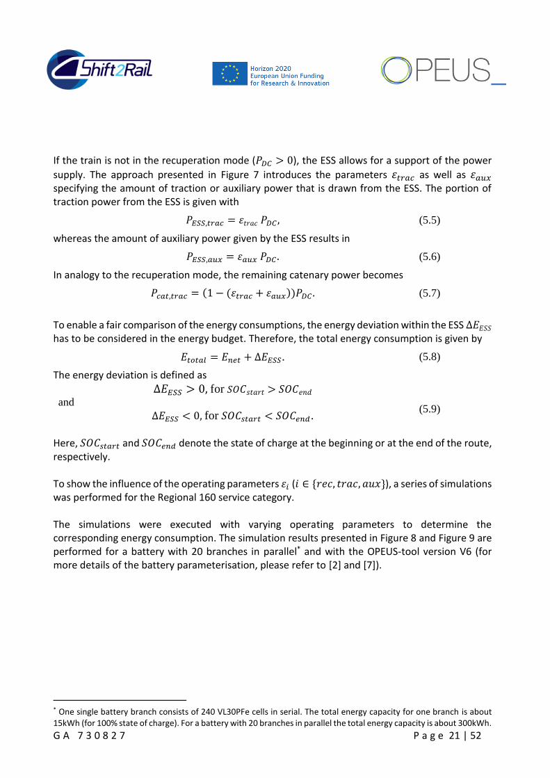
Here, 𝑆𝑂𝐶𝑠𝑡𝑎𝑟𝑡 and 𝑆𝑂𝐶𝑒𝑛𝑑 denote the state of charge at the beginning or at the end of the route, respectively. To show the influence of the operating parameters 𝜀𝑖 (𝑖 ∈ {𝑟𝑒𝑐, 𝑡𝑟𝑎𝑐, 𝑎𝑢𝑥}), a series of simulations was performed for the Regional 160 service category. The simulations were executed with varying operating parameters to determine the corresponding energy consumption. The simulation results presented in Figure 8 and Figure 9 are performed for a battery with 20 branches in parallel* and with the OPEUS-tool version V6 (for more details of the battery parameterisation, please refer to [2] and [7]).

* One single battery branch consists of 240 VL30PFe cells in serial. The total energy capacity for one branch is about 15kWh (for 100% state of charge). For a battery with 20 branches in parallel the total energy capacity is about 300kWh.


G A 7 3 0 8 2 7 P a g e 22 | 52

Figure 8: Energy simulation results for varying ESS operating parameters 𝜺𝒕𝒓𝒂𝒄, 𝜺𝒂𝒖𝒙 and a fixed

recuperation parameter 𝜺𝒓𝒆𝒄 (Reg160)

Figure 9: State of charge at the end of the drive cycle for varying ESS operating parameters 𝜺𝒕𝒓𝒂𝒄,

𝜺𝒂𝒖𝒙 and a fixed recuperation parameter 𝜺𝒓𝒆𝒄 (Reg160)

Figure 8 depicts the resulting energy consumption according to equation (9.8). Here, the green surface represents the baseline value, whereas the yellow and red surfaces are the simulation

results for either 𝜀𝑟𝑒𝑐 = 1 (yellow – total recuperation to the battery) or for 𝜀𝑟𝑒𝑐 = 0 (red – no recuperation to the battery). As indicated in Figure 8 and Figure 9, the increase of the operating battery parameters leads to an improvement in the energy consumption - as long as the battery is not discharged to the minimum


G A 7 3 0 8 2 7 P a g e 23 | 52

state of charge (here 𝑆𝑂𝐶𝑚𝑖𝑛 = 0.1). To allow for a balanced battery SOC, the battery has to be charged at the end of the route. This scenario is described in more detail in Section 5.2. Further research within the course of OPEUS (esp. WP 6) will utilise the presented approach to develop energy optimal operating strategies for the ESS in order to investigate the utilisation scenarios for the defined service categories.

5.2 Scenario simulations with energy storage systems In this chapter, each simulation in the presence of an ESU battery is performed with the version 2 of the OPEUS-tool. That may cause some differences with reference to the energy summary in chapter 4 and chapter 6, which was calculated with version 6 of the OPEUS-tool. The main initial conditions (general inputs) are as follows:

At rail vehicle level: o Type of rail vehicle: Reg160 o Track profile: Reg160 o Trajectory mode: allout o Season mode: winter o Partial switch-off of traction components: off o Partial load distribution: off o Topology: T01 (AC power supply)

At ESS level:

o ESS-DLC: no double layer capacitor presence o ESS-battery: 1 ESU-battery integrated o Cell technology for Anode/Cathode active material: Super Iron Phosphate

(sLFP)/Graphite o Initial state of charge: 80% o A single battery branch consists of 240 VL30PFe cells in serial o Total energy capacity for a single battery branch: about 15kWh (at 100% SoC)

Four scenarios are considered for the Regional 160 service category as defined in Table 3. The two last scenarios (*) were discussed and agreed with SNCF (member of the cooperation project FINE1). For the scenarios II, III and IV, the charging of the battery is achieved by the utilisation of regenerative braking. Furthermore, all these three scenarios uses the battery power to compensate for the auxiliary power request. For all scenarios with an ESU, the SOC of the battery has to be balanced at the start and the end of the route. This approach ensures a fair comparison between the baseline scenario and the ESU-scenarios. The maximum time to recharge the battery up to its initial SOC should be limited to a maximum charging time of 15 minutes.


G A 7 3 0 8 2 7 P a g e 24 | 52

Scenario Main description

battery size in branch //

1 branch configuration

I Without ESS Baseline scenario - -

II ESU included - SOC balancing at the end of the course

battery charge during braking phase; permanent discharge for auxiliaries

20 240 VL30PFe cells in serial

III ESU included – SOC balancing at the end of the course and partial electrification (geometric approach) *-discussed with SNCF

battery charge during braking phase; permanent discharge for auxiliaries and for four defined non-electrified sections

2

IV ESU included – SOC balancing at the end of the course with 25% of traction power request (peak shaping approach)

*-discussed with SNCF

battery charge during braking phase; permanent discharge for auxiliaries and for 25% of the traction power request

20

Table 3: Considered scenarios with the presence of ESU-battery

In the partial electrification scenario (scenario III), the battery is discharged if necessary during the four non-electrified zones defined in the discussion with SNCF, see Figure 10.

Figure 10: Definition of four non-electrified zones with constant vehicle speed: train position in

km (blue curve), train speed in km/h (red curve)


G A 7 3 0 8 2 7 P a g e 25 | 52

Figure 11 shows the electrical power of the ESU-battery (𝑃𝑏𝑎𝑡 > 0 in discharge mode, 𝑃𝑏𝑎𝑡 < 0 in charge mode) and its SOC for scenario III.

Figure 11: Electrical power (red curve) and SOC (blue curve) of the ESU-battery

Four power peaks - corresponding to the four non-electrified zones where the train takes the full traction energy from the ESU-battery to ensure a constant speed - interrupt the constant portion of battery power that covers the auxiliary power supply. In the fourth scenario (peak shaping approach), 25% of the traction power requirement is delivered by the ESU-battery to make sure that at the end of the course (before recharging) the battery reaches its minimum SOC of 10%. The most prominent advantage of this approach is the possibility to decrease the power peaks at the catenary, especially during acceleration phases and the consequent energy savings. Figure 12 shows that scenario III (with non-electrified zones) provides almost the same traction energy at the catenary level. Furthermore, the recuperated energy in this scenario is slightly lower than the one of the reference scenario. Using the ESU-battery in this scenario could considerably improve the flexibility of the train in cases where the installation of an electrical infrastructure would be hard to realise or too expensive.


G A 7 3 0 8 2 7 P a g e 26 | 52

Figure 12: Traction energy (in kWh) calculated at the catenary

Figure 13: Recuperated energy (in kWh) to the catenary

According to Figure 13, the recuperated energy at catenary in scenario II and the scenario IV is significantly lower in comparison to the reference scenario as well as scenario III. The reason for this deviation is the required energy to recharge the battery with 20 branches in parallel. All the three scenarios with an ESU-battery comply with the maximum time limit (15 mins) to recharge the battery up to the initial SOC, Figure 14:


G A 7 3 0 8 2 7 P a g e 27 | 52

Figure 14: Charging time (in minutes) of the battery at the end of the course

5.3 Optimized ESS management This section presents the simulation results for an ESS operating strategy with parameters, determined by an optimisation algorithm. The cost function J for the energy optimal operating strategy is formulated as

𝐽𝐸𝑆𝑆 = 𝐸𝑛𝑒𝑡 + Δ𝑆𝑜𝐶2, (5.10)

with Δ𝑆𝑜𝐶 = 𝑆𝑜𝐶𝑠𝑡𝑎𝑟𝑡 − 𝑆𝑜𝐶𝑒𝑛𝑑. The minimisation of the above cost function determines the ESS operating parameters for an energy optimal application of the ESS in combination with a balanced 𝑆𝑜𝐶 at the beginning and at the end of the drive cycle. This optimisation is paradigmatically applied for the HS250 service, the Regional 160 service, the Freight Mainline service as well as for the Tram and Metro service. The operating parameters for the presented scenario are determined by an optimisation algorithm in order to solve the optimisation problem (5.10). Here, the recuperation factor 𝜀𝑟𝑒𝑐 is fixed to 𝜀𝑟𝑒𝑐 =1, which allows for a maximum recuperation effort into the ESS. The size of the battery (number of parallel branches) is fitted to the power request of the single service profiles. With the selected battery size, the evolution of the resulting state of charge is well balanced around 𝑆𝑜𝐶~50% (initial state: 𝑆𝑜𝐶(𝑡0) = 50%). The main initial conditions for the simulation results below are summarised in Table 4.


G A 7 3 0 8 2 7 P a g e 28 | 52

Table 4: ESS operating parameters

Service

profile

ESS operating strategy Battery size – Number

of branches in parallel 𝜀𝑟𝑒𝑐 𝜀𝑡𝑟𝑎𝑐 𝜀𝑎𝑢𝑥

HS250 1* 2% 5% 10

Reg160 1* 3% 7% 5

Tram 1* 5% 11% 1

Metro 1* 3.5% 28% 1

FrMain 1* 2.5% 48% 10

* Recuperation factor 𝜺𝒓𝒆𝒄 = 𝟏 to allow for a maximum recuperation into the ESS

According to the resulting operating parameters from Table 4, the traction supply from the ESS is nearly disabled (0%...3% power supply for the traction came from the ESS), as the ESS delivers about 14%-48% of the auxiliary power. In consequence of the additional ESS mass, the velocity trajectories for an ESS loaded vehicle are determined. The resulting velocity trajectory is slightly different according to the baseline speed profiles and is applied for the ESS simulations. This effect also leads to deviations at the energy balance at the wheel, which is considered in the following results. However, the deviations within the velocity profiles are too small for a proper representation in the following figures. Therefore, only the baseline velocity profile is depicted.


G A 7 3 0 8 2 7 P a g e 29 | 52

Table 5: Simulation results for ESS application (balanced SoC) for HS250 service

Figure 15: Velocity trajectory and State-of-Charge for HS250 service

Figure 16: Power profile at the ESS (balanced SoC) for HS250 service

Figure 17: Power profile at the catenary for ESS application (balanced SoC) for HS250 service

Baseline ESS usage

Traction energy at the wheel [kWh] 2850 2864

Braking energy at the wheel [kWh] 655 667

Consumed energy at the catenary [kWh] 4414 4314

Recuperated energy at the catenary [kWh] 220 121

Difference of energy stored in ESS [kWh] - -7

Total net energy [kWh] 4194* 4201*

Total energy savings in kWh -7

Total energy savings in % about -0.2

*The total net energy is determined with non-rounded values


G A 7 3 0 8 2 7 P a g e 30 | 52

Table 6: Simulation results for ESS application (balanced SoC) for Reg160 service

Figure 18: Velocity trajectory and State-of-Charge for Reg160 service

Figure 19: Power profile at the ESS (balanced SoC) for Reg160 service

Figure 20: Power profile at the catenary for ESS application (balanced SoC) for Reg160 service

Baseline ESS usage








Total energy savings in % about -1



G A 7 3 0 8 2 7 P a g e 31 | 52

Table 7: Simulation results for ESS application (balanced SoC) for Tram service

Figure 21: Velocity trajectory and State-of-Charge for Tram service

Figure 22: Power profile at the ESS (balanced SoC) for Tram service

Figure 23: Power profile at the catenary for ESS application (balanced SoC) for Tram service

Baseline ESS usage








Total energy savings in % about -2



G A 7 3 0 8 2 7 P a g e 32 | 52

Table 8: Simulation results for ESS application (balanced SoC) for Metro service

Figure 24: Velocity trajectory and State-of-Charge for Metro service

Figure 25: Power profile at the ESS (balanced SoC) for Metro service

Figure 26: Power profile at the catenary for ESS application (balanced SoC) for Metro service

Baseline ESS usage






Total net energy [kWh] 268 272


Total energy savings in % about -1.5



G A 7 3 0 8 2 7 P a g e 33 | 52

Table 9: Simulation results for ESS application (balanced SoC) for Freight Mainline service

Figure 27: Velocity trajectory and State-of-Charge for Freight Mainline service

Figure 28: Power profile at the ESS (balanced SoC) for Freight service

Figure 29: Power profile at the catenary for ESS application (balanced SoC) for Freight service

Baseline ESS usage






Total net energy [kWh] 5254 5333


Total energy savings in % about -1,5



G A 7 3 0 8 2 7 P a g e 34 | 52

The simulation results above present the application of the optimised operating strategy for the ESS. Despite the additional mass of the battery, the total net energy of the presented drive cycles is not increased significantly. The major advantage of the presented ESS application is the decrease of the net power peaks (peak shaving approach). For the positive power flow, the ESS delivers almost constant power supply with just minor supply for traction power peaks (see Figure 16, Figure 19, Figure 23 and Figure 28). During the recuperation mode, however, the ESS provides the possibility for a recuperation, which allows for a substantial peak reduction. The maximum recuperation power peaks for the presented service categories are summarised in Table 10*.

Table 10: Power peak reduction during recuperation due to ESS application

Maximum recuperation power peak at the net - baseline

Maximum recuperation power peak at the net – ESS application

Power peak reduction in %

High Speed 250 -3603kW -2406kW 33%

Regional 160 -1845kW -1245kW 32,5%

Tram -709kW -586kW 18%

Metro -5487kW -4860kW 12%

Freight Mainline -1980kW -1980kW* 0%* *for the Freight Mainline application, the maximum power peak is equal to the baseline result, as there is a

state, when the ESS is charged to the maximum SoC and does not allow for a further recuperation

The simulations results presented in this section, show the benefit of the ESS application regarding reduced net energy peaks. Furthermore, it shows the application of an optimisation technique to determine a proper operating strategy. For further investigations within OPEUS WP6, the cost function defined in (5.10) can be adjusted in order to fulfil further scenario specifications. Additionally, the definition and simulation of further ESS scenarios are part of the further progress of OPEUS WP6 and will be reported in the corresponding report of WP6 as well as in the final report of WP7, which covers the global vision of railway energy usage. For example, another approach is considered for mainline lines with several non-electrified zones where the infrastructure cost is very high (geographic approach). Simulations for this scenario for the Regional 160 service are already evaluated. Furthermore, scenarios with intermediate recharging of the battery at the stations are

considered within the further simulation studies of WP6.

* Note: The capability of recuperate power peaks is closely related to the size of the battery. The values presented in Table 10 only are applicable for the battery sizes presented in Table 4. The influence of the battery size is under further investigations within the work done in WP6.


G A 7 3 0 8 2 7 P a g e 35 | 52

6 Driving strategy improvements This section gives an introduction to the investigations of driving strategies that are considered within WP4 of OPEUS. This current section focuses on the general impact of coasting on the energy consumption of the defined service categories. Therefore, two different trajectory modes are evaluated (see Figure 30).

Figure 31: Possible trajectory modes

The first trajectory mode uses coasting to fulfil the timetable and is structured as follows (according to the green line in Figure 32):

1. Acceleration phase with max. acceleration (limited by the max. traction effort and the passenger comfort) until a defined speed limit 𝑣𝑙𝑖𝑚 is reached;

2. Cruising (const. speed), if necessary; 3. Coasting to fulfil the time-table; 4. Braking with max. deceleration (limited by the max. braking effort and the passenger

comfort). Here, a bisection algorithm determines the starting position for the application of coasting. The second trajectory mode does not utilise coasting. Therefore, this trajectory mode is characterised by the following three steps (according to the red line in Figure 33):

1. Acceleration phase with max. acceleration (limited by the max. traction effort and the passenger comfort) until a desired speed 𝑣𝑑 is reached;

2. Cruising (const. speed); 3. Braking with max. deceleration (limited by the max. braking effort and the passenger

comfort). In analogy to the first trajectory mode, a bisection algorithm is used as well to determine the

proper velocity 𝑣𝑑 that meets the timetable.


G A 7 3 0 8 2 7 P a g e 36 | 52

The total net energy consumption (according to equation (3.1)), as well as the relative energy saving with reference to coasting, is shown in Figure 34

Figure 35: Relative energy savings based on the implementation of coasting and the total net

energy consumption for both trajectory modes

For almost each service category, the utilisation of coasting reduces the energy consumption (at least by a few percentage points). However, the High Speed 300 service is an exception, which uses more energy when the coasting mode trajectory is employed. These energy consumptions are the result of two contrary effects:

On the one hand, coasting utilises the effect that the vehicle behaves as natural energy

storage for kinetic energy. The use of this kinetic energy during coasting enables to cover

a significant part of the track without any external traction power;

On the other hand, the coasting mode requires high vehicle speeds which can be explained

by the quadratic dependency of the kinematic energy on the speed. This high vehicle

speeds, however, leads to higher energy losses caused by the aerodynamic resistance.

The focus of further work within OPEUS WP4 is an improvement of these driving strategies to derive a driving strategy with efficient energy consumption that allows for an optimal trade-off between these two contrary effects.

-8.0

-6.0

-4.0

-2.0

0.0

2.0

4.0

6.0

8.0

ener

gy s

avin

gs in

%

0

1000

2000

3000

4000

5000

6000

HS300 HS250 Intercity Regional160

Regional140

Suburban Metro Tram FreightMain

tota

l en

ergy

in k

Wh

No Coasting

With Coasting (baseline)


G A 7 3 0 8 2 7 P a g e 37 | 52

The objective of this section is the summary of the simulation results regarding the driving strategy improvements investigated within WP4 of OPEUS. The work within WP4 focuses on the determination of an optimal energy driving strategy in order to implement the optimal velocity profile in form of a driver assistant system (DAS). As already explained earlier, and in [2], the baseline trajectory planner bases on a heuristic approach, which tries to maximise the amount of coasting under the consideration of given constraints. Consequently, the benchmark speed profile is characterized by the green curve in Chapter 3, Figure 1). This baseline speed profile is not the most energy efficiency driving style for all scenarios. Therefore, the current work focuses on the determination of the driving style, which combines the usage of coasting and the avoidance of high speed for the energy optimal solution, respecting always the boundary conditions (timetable and speed restrictions). The theoretical background for the applied optimisation approach is given within Section 6.1, whereas Section 6.3 focuses on the influence of gradients for the potential for DAS/ATO operation. The simulation results are summarised in Section 6.2. Section 6.4 closes Chapter 6 with a short outlook for the future work regarding DAS/ATO operation.

6.1 Optimisation approach for the energy-optimal driving strategy As already introduced, and also in [2], the driving strategy is determined for every single section (station to station drive). The corresponding optimisation parameters, which determine the driving style are summarized in Figure 36 (for a more detailed description of the trajectory planner, please see [2], [8] and [9]).

Figure 36: Driving strategy parameters


G A 7 3 0 8 2 7 P a g e 38 | 52

The insertion point for coasting 𝑠𝑐 is given by

𝑠𝑐 = 𝑏𝑐𝑠𝑒𝑛𝑑, (6.1)

with the optimisation parameter 𝑏𝑐 and the total distance 𝑠𝑒𝑛𝑑. The maximum speed of the section 𝑣𝑑 is determined by

𝑣𝑑 = 𝑝𝑣𝑎𝑣𝑙𝑖𝑚, (6.2)

where 𝑝𝑣𝑎 is the corresponding optimisation parameter and 𝑣𝑙𝑖𝑚 represents the speed limit of the current section. The variation of the optimisation parameters 𝑏𝑐 and 𝑝𝑣𝑎 leads to different driving velocity profiles, presented in Figure 37. The constraints of these velocity profiles are given by the required timetables, which are characterised via the position and time at the beginning (𝑠0, 𝑡0) and at the end (𝑠𝑒𝑛𝑑, 𝑡𝑒𝑛𝑑) of the section. As introduced earlier in this deliverable, the usage of coasting is the major influence regarding the energy consumption. Figure 37 summarizes the extreme cases:

The green curves present the velocity profiles with the maximum amount of coasting – for

a speed profile without speed limit restriction, this is given for the optimisation

parameter 𝑏𝑐 = 0.

The red curves mark the speed profiles without any coasting utilisation (𝑏𝑐 = 1). The speed

profile is adjusted only via the optimisation parameter 𝑝𝑣𝑎 (with 𝑝𝑣𝑎 < 1).

Figure 37: Possible driving styles to fulfil the timetable

To determine the most energy efficient driving style, the OPEUS tool and the included trajectory planner (see [1] and [2]) are applied to calculate the velocity profiles as well as the corresponding energy consumptions. Based on the simulation results, the cost function for the optimisation approach can be stated with:

𝐽𝐷𝑆 = 𝐸𝑛𝑒𝑡 + 𝛼𝑠 ∙ 𝑐𝑜𝑛𝑠 + 𝛼𝑡 ∙ 𝑐𝑜𝑛𝑠. (6.3)


G A 7 3 0 8 2 7 P a g e 39 | 52

Here, 𝐸𝑛𝑒𝑡 is defined by equation (3.1) and the further terms (𝛼 𝑠 ∙ 𝑐𝑜𝑛𝑠, 𝛼 𝑡 ∙ 𝑐𝑜𝑛𝑡) are weighted penalty costs to ensure the compliance with the position and time constraints of the required timetable. To determine the energy optimal velocity profile, the optimisation problem for the driving style

min𝑏𝑐,𝑝𝑣𝑎

𝐽𝐷𝑆 (6.4)

has to be solved. For this purpose, different optimisation algorithms (CMA-ES – Co-variance matrix adaption – evolution strategy [11], PSO – particle swarm optimisation [12], GWO – grey wolves optimiser [13], FFA – firefly algorithm [14]) are applied and the solutions are compared. Information about the detailed optimisation problem as well as details about the optimisation algorithms are not part of this deliverable. This content will be expounded in more detail in the deliverable D4.2 - Driving strategies and energy management for DAS of WP4.

6.2 Simulation results for energy optimised velocity profiles This section presents the energy simulation results for the velocity profiles, determined by the optimisation algorithms mentioned above. These investigated optimisation approaches are compared and the most energy efficient solution is presented in the current section. Furthermore, it follows for several service profiles, that the baseline velocity profile (presented in [3]) already presents the most energy efficient driving style. For these service categories the evaluation of the optimisation algorithms delivers nearly the same velocity profiles, as determined by the heuristic baseline approach, which is based on the maximisation of coasting. Namely these service categories are:

Intercity service

Regional 160 service

Regional 140 service

Suburban service

Metro service

Tram service

Conclusively, this section presents only the service profiles, which show benefit of the optimised driving strategy. The improved service categories are listed below:

High Speed 300 service

High Speed 250 service

Freight Mainline

For an easy assessment, the energy consumption is considered for every section. This allows for an interpretation, in which section the major energy savings are achieved.


G A 7 3 0 8 2 7 P a g e 40 | 52

Table 11: Simulation results for energy optimised velocity trajectory for HS300 service

Figure 38: Baseline and energy optimised velocity trajectories for HS300 service

Figure 39: Power profile at the catenary for optimised driving strategy for HS300 service

Net energy [kWh] - baseline Net energy [kWh] - optimised trajectory (CMA-ES)

Station A-B 1013 990

Station B-C 4042 3652

Total net energy 5055 4642

Total energy savings in kWh 413

Total energy savings in % 8,2


G A 7 3 0 8 2 7 P a g e 41 | 52

Table 12: Simulation results for energy optimised velocity trajectory for HS250 service

Figure 40: Baseline and energy optimised velocity trajectories for HS250 service

Figure 41: Power profile at the catenary for optimised driving strategy for HS250 service


Station A-B 945 902


Station C-D 1157 1163

Station D-E 1011 960



Total energy savings in % 2,1


G A 7 3 0 8 2 7 P a g e 42 | 52

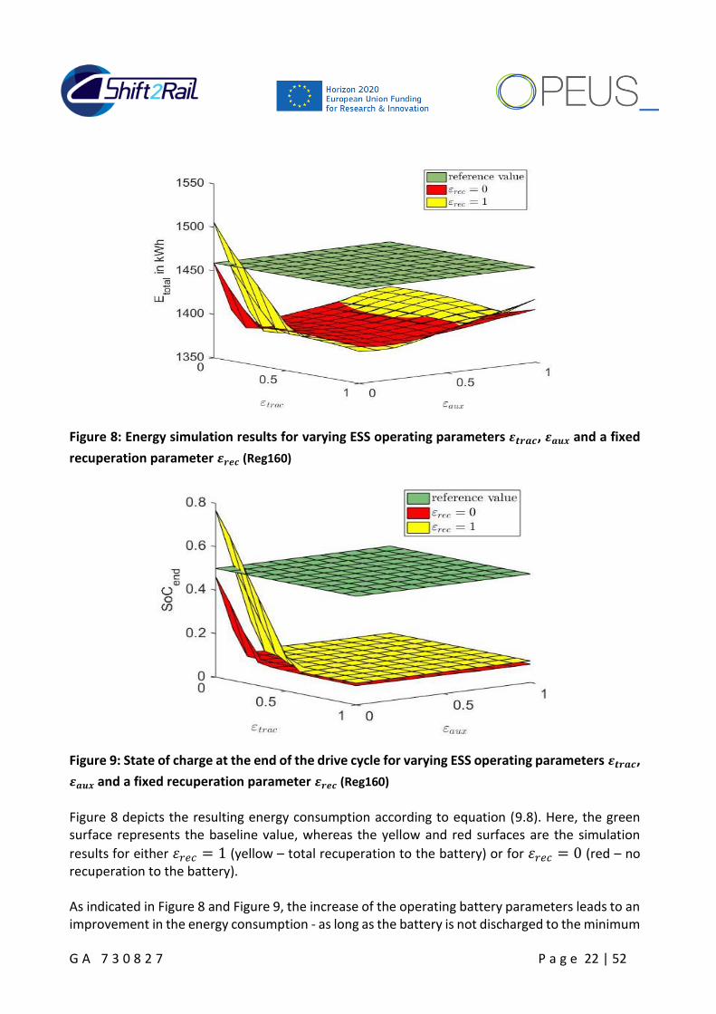
Table 13: Simulation results for energy optimised velocity trajectory for Freight Mainline service

Figure 42: Baseline and energy optimised velocity trajectories for Freight Mainline service

Figure 43: Power profile at the catenary for optimised driving strategy for Freight Mainline


Station A-B 240 240


Station C-D 337 322

Station D-E 1814 1807

Station E-F 1685 1558

Station F-G 152 152



Total energy savings in % about 4


G A 7 3 0 8 2 7 P a g e 43 | 52

The simulation results presented above show a potential energy saving up to 8% with the usage of energy optimal driving strategies. Especially for the HS300 as well as for the Freight Mainline service, it shows that the avoidance of high vehicle speed has a positive effect on the total energy consumption. This is caused by a long state with constant speed and a high power request – see Figure 39 (𝑠 ∈ [130km … 250km]) for High Speed 300 and Figure 43 (𝑠 ∈ [200km … 280km]) for Freight Mainline. For the High Speed 250 service this effect is not that pronounced, as there are not such long constant high speed sections. As the baseline service profiles are defined without gradients (except Freight Mainline), the presented optimal velocity profiles are only valid for flat track profiles. To assess the influence of gradients, the next section covers a series of simulations for different gradient scenarios.

6.3 Influence of gradients The major potential for the optimal driving strategy application is to be expected for tracks with gradients included. The consideration of the gradient data for the determination of the energy optimal velocity trajectory, enables the usage of the train mass as an additional energy storage: The increased kinetic energy of the train (caused by increased velocity of the train during downhill sections) will be used to reduce the traction power for uphill sections. For that purpose representative gradients are applied for the below service categories. These service profiles are either forwarded from IMPACT1 (Grant Agreement number: 730816) via the FINE1 energy group, or are defined within OPEUS WP4:

High Speed 300 service – from IMPACT (SPD1) via FINE1

Regional 140 service – from IMPACT (SPD2) via FINE1

Metro service – from IMPACT (SPD3) via FINE1

Tram service – defined within WP4 by Stadler

Freight Mainline service – defined within baseline scenario

To allow for a fair assessment of the gradient influence, three different gradient scenarios will be compared within this section:

I. No gradient – Flat section:

This scenario covers a flat track profile and therefore the gradient is not considered within

the trajectory planning. Except for Freight Mainline, this scenario is equivalent to the

reference scenario.

II. Baseline velocity trajectory – Unknown gradient:

For this scenario the gradient is to be considered as unknown. Therefore, the trajectory

planner does not consider the gradient profile. Conclusively, the velocity profile which is

determined for the flat profile is simulated for the track profile fraught with gradients. The

simulations results for that scenario underline that the unknown gradient has a special

effect for the sections, where the trajectory planner (for the flat section) scheduled


G A 7 3 0 8 2 7 P a g e 44 | 52

coasting. Here, a pure ‘zero-power’ coasting is not applied, to fulfil the requested speed

profile.

III. Gradient considered for the trajectory planning

The third scenario considers the gradient profile for the trajectory planning. The trajectory

planner includes the information of the altitude profile for the determination of the

velocity profile. The resulting velocity profile reflects this gradient influence.

For all scenarios the velocity profiles are determined by the heuristic trajectory planner, which is based on the maximisation of coasting (see Section 6). The implementation of the optimisation algorithms explained above, however, have not yet been applied for the gradient track profiles. This is part of further investigations within OPEUS WP4. For the assessment of the influence of the gradient the simulation results of the total net energy for the scenario II and scenario III (both represent a gradient based track profile) are compared. To avoid a not expedient comparison of a flat track profile with a gradient track profile, the two scenarios represent simulation scenarios with gradients included.


G A 7 3 0 8 2 7 P a g e 45 | 52

Table 14: Simulation results for gradient influence for HS300 service

Figure 44: Velocity trajectories for HS300 track profile with and without gradient

Figure 45: Power profile at the catenary for various gradient scenarios for HS300 service

Net energy in kWh: Flat profile (baseline)

Net energy in kWh: Gradient NOT considered for trajectory planning

Net energy in kWh: Gradient considered for trajectory planning

Station A-B 1013 1296 1311

Station B-C 4042 3376 3636

Total net energy 5055 4672 4947

Total energy savings in kWh - -275

Total energy savings in % - about -6


G A 7 3 0 8 2 7 P a g e 46 | 52

Table 15: Simulation results for gradient influence for Reg140 service

Figure 46: Velocity trajectories for Reg140 track profile with and without gradient

Figure 47: Power profile at the catenary for various gradient scenarios for Reg140 service

Figure 48: Power profile at the catenary for various gradient scenarios for Reg140 service -

extract





Total energy savings in kWh

- 7

Total energy savings in % - about 1.5


G A 7 3 0 8 2 7 P a g e 47 | 52

Table 16: Simulation results for gradient influence for Metro service

Figure 49: Velocity trajectories for Metro track profile with and without gradient

Figure 50: Power profile at the catenary for various gradient scenarios for Metro service

Figure 51: Power profile at the catenary for various gradient scenarios Metro service -

extract





Total energy savings in kWh - 2

Total energy savings in % - about 1


G A 7 3 0 8 2 7 P a g e 48 | 52

Table 17: Simulation results for gradient influence for Tram service

Figure 52: Velocity trajectories for Tram track profile with and without gradient

Figure 53: Power profile at the catenary for various gradient scenarios for Tram service





Total energy savings in kWh - 0

Total energy savings in % - 0


G A 7 3 0 8 2 7 P a g e 49 | 52

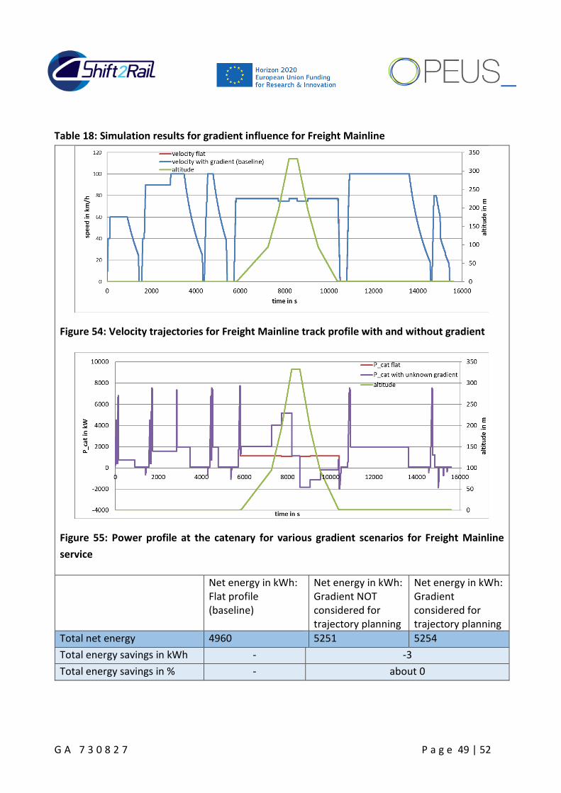
Table 18: Simulation results for gradient influence for Freight Mainline

Figure 54: Velocity trajectories for Freight Mainline track profile with and without gradient

Figure 55: Power profile at the catenary for various gradient scenarios for Freight Mainline

service





Total energy savings in kWh - -3

Total energy savings in % - about 0


G A 7 3 0 8 2 7 P a g e 50 | 52

The simulations results above present the influence of the gradient regarding the resulting power profile at the energy source as well as the influence on the total net energy. On the basis of the total net energy results, there is no unambiguous assessment for either a benefit or a disadvantage of the gradient influence. This is mainly based on the diversity of the investigated track profiles. Not only the general characteristic of the gradient profile (e.g. start altitude, end altitude, maximum slopes, etc.) has an effect on the total net energy, but also the correlation of the velocity profile and the gradient profile is a major parameter. For example for the HS300 service, the coasting phases of the speed profile almost correlates to uphill sections of the gradient profile (see Figure 44, time ∈ [1500s … 2500s] ∪ [5000s … 6500s]), which has a negative influence regarding the net energy. The same effect is emphasised within the right half of Figure 51: The power profile, which is based on scenario III (gradient known – red curve), represents a coasting phase, as the purple power characteristic (unknown gradients) is increased in order to fit the requested velocity profile. The simulation results for Regional 140, Metro, Tram and Freight Mainline are almost balanced for the scenario comparison. Here, benefits and disadvantages of the gradient neglected each other over the sum of the total track distance. Especially for the Freight Mainline application this is obvious, as the trajectory planner determines almost equal velocity profiles for both the known as well as for the unknown gradient profile. In summary, the simulation results show that an assessment of the gradient influence is difficult as long as only the total net energy of the total drive cycle is considered, and if comparison of gradient profiles with flat profiles are made. This is caused by the diversity of the combinations of gradient profiles and a proper velocity trajectories. What is expected is that when the energy optimization strategies explained in 6.2 are applied in services profiles with gradients the benefits (compared to baseline simulations on services profiles with gradients) are greater than when these strategies are applied in flat service profiles, this will be shown in deliverable D4.2. In addition, for a proper analysis, the station by station energy values as well as the detailed power profile have to be considered. Furthermore, the correlation of the gradient profile and the resulting velocity profile has to be analysed.

6.4 DAS outlook to deliverable DO3.3 - part 3 This section addresses the further investigations regarding the driving style application. As mentioned above, simulations will be performed to apply the optimisation algorithms for gradient based tracks. Furthermore, there is an expansion of the driving strategy under investigation, which allows for multiple coasting applications during the drive cycle instead of only one coasting usage at the end of the station.


G A 7 3 0 8 2 7 P a g e 51 | 52

7 Conclusion This deliverable report describes the first energy simulations evaluated within the progress of OPEUS. These simulations were executed in order to assess the influence of the technical innovations, which are under investigation within the OPEUS work packages WP4 (driver assistance systems), WP5 (in-vehicle losses analyses) and WP6 (ESS-studies). To explain the background of the simulation results, the theoretical background underlying the investigated technical innovations is explained. Furthermore, the baseline scenario is presented and the baseline results are summarised. The evaluated simulation results of the investigated techniques are compared to the baseline results in order to assess the influence regarding the in-vehicle energy usage. Summing up, this work indicates further developments in the work packages WP4, WP5 and WP6 of OPEUS and contributes to a global vision of energy usage in railways, developed in WP7. The second part of this deliverable series (D03.4) is going to resume the presentation of simulation results regarding the investigations of OPEUS. Furthermore, additional Shift2Rail innovations will be evaluated using the OPEUS tool. The corresponding data gathering is performed by FINE1 in the framework of FINE1 Task 4.2 – Data Gathering.


G A 7 3 0 8 2 7 P a g e 52 | 52

8 References

[1] L. Pröhl, „OPEUS Deliverable - DO2.3 OPEUS simulation tool manual,“ EU-project OPEUS (S2R-OC-CCA-02-2015), 2017.

[2] L. Pröhl, „OPEUS Deliverable DO2.1 - OPEUS simulation methodology,“ EU-project OPEUS (S2R-OC-CCA-02-2015), 2017.

[3] L. Pröhl, „OPEUS Deliverable DO3.2 - Baseline simulation results and assessment,“ EU-project OPEUS (S2R-OC-CCA-02-2015), 2018.

[4] R. Palacin, „OPEUS Deliverable DO3.1 - Scenario set up and discription,“ EU-project OPEUS (S2R-OC-CCA-02-2015), 2017.

[5] J. Ernst, „FINE1 Deliverable D3.1 - Energy baseline,“ EU-project FINE1 (S2R-CFM-CCA-02-2015), 2018.

[6] H. Dittus, „FINE1 Deliverable D3.4 - Requirement specification for energy simulation tool,“ EU-project FINE1 (S2R-CFM-CCA-02-2015), 2017.

[7] D.-A. Nguyen, „CleanER-D Deliverable 7.4.3 - Basic electrochemistry modular proposal and specifications,“ EU-project CleanER-D (project 234338), 2011.

[8] L. Pröhl, „OPEUS Deliverable DO3.3 - S2R innovation (state01) simulation results and periodic assessmant - Part1,“ EU-project OPEUS, 2018.

[9] M. Leska, "CleanER-D Deliverable DEL7.3.3 - Model-based prediction of fuel consumption and estimation of corresponding emissions," EU-project CleanER-D (project 234338), 2012.

[10] M. Leska, Berechnung kraftstoffoptimaler Trajektorien und Betriebsstategien für DIesel-Hybrid-Schienenfahrzeuge (in German), PhD thesis, University of Rostock. Aachen: Shaker Verlag, 2016.

[11] N. Hansen und A. Ostermeier, „Completely Derandomized Self-Adaption in Evolution Strategies,“ Evolutionary Computation, Nr. 9(2), pp. 159-195, 2001.

[12] J. Kennedy und R. Eberhart, „Particle Swarm Optimization,“ IEEE, Perth, Australia, 1995.

[13] S. Mirjalili, S. M. Mirjalili und A. Lewis, „Grey Wolf Optimizer,“ Advances in Engineering Software, Nr. 69, pp. 46-61, 2014.

[14] X.-S. Yang, „Firefly Algorithm for Multimodal Optimization,“ in Stochastic Algorithms: Foundations and Applications , Sapporo, Japan, Springer, 2009, pp. 169-178.


Deliverable D 3.3 S2R innovation first periodic assessment

Documents

Transcript of Deliverable D 3.3 S2R innovation first periodic assessment