Deliverable # 2.2: Seismically induced hazards, failure ...

Project n°: 691213 H2020-MSCA-RISE-2015

Project Acronym: EXCHANGE-RISK

Project Full Name: EXperimental Computational Hybrid Assessment of Natural Gas pipelines Exposed to Seismic Risk

Marie Skłodowska - Curie Actions

Deliverable # 2.2: Seismically induced hazards, failure modes and limit states and performance indicators of

NG pipelines.

Period number: 1

Start date of project: 01/01/2016

Project coordinator name: Anastasios Sextos

Project coordinator organisation name: University of Bristol

Date of preparation: 31/12/2016

Date of submission (SESAM): 17/1/2017

Nature: Report

Version: 1.0

Ref. Ares(2017)3456039 - 09/07/2017

691213 H2020-MSCA-RISE-2015 Deliverable #<2.2>

2

Institutions Involved (Work Package 02 <D2.2>)

1. UNIVERSITY OF BRISTOL

2. BAUHAUS-UNIVERSITAET WEIMAR

3. ARISTOTELIO PANEPISTIMIO THESSALONIKIS

4. UNIVERSITA DEGLI STUDI DEL SANNIO

5. UNIVERSITY OF PATRAS

6. CHRISTIAN-ALBRECHTS-UNIVERSITAET ZU KIEL

7. THE GOVERNING COUNCIL OF THE UNIVERSITY OF TORONTO

Authors:

Anastasios G. Sextos, Associate Professor, Reader (UOB)

Psyrras Nikolaos, Ph.D. Candidate (UOB)

Lead institution for the preparation of Deliverable # 2.2:

University of Bristol


3

This document contains contributions made in the framework of the research program H2020-

MSCA-RISE-2015. The disclosure, publication and use of the information and data provided to

third parties is not allowed, unless compliant to the provisions of the consortium agreement.


4

Table of Contents

1 Introduction ........................................................................................................ 6

2 Dynamic soil-pipe interaction ........................................................................... 8

2.1 Models ignoring soil-pipe interaction ............................................................................................. 8

2.2 Models with account for soil-pipe interaction ................................................................................ 9

3 Predicting spatially variable transient ground motions along the pipeline 17

4 Dominant failure modes and supporting evidence from past earthquakes 20

5 Fragility expressions for buried pipelines ...................................................... 25

6 Pipeline health monitoring for maintenance and rehabilitation .................. 31

7 The emerging concept of resilience in pipeline networks ............................. 37

8 Current codes of practice and guidelines for earthquake-resistant design of

buried pipelines ................................................................................................ 41

9 Discussion and conclusions .............................................................................. 46

Acknowledgements ................................................................................................. 47

References ............................................................................................................... 48


5

Seismic resilience of buried steel natural gas pipelines

Abstract. Experience has shown that earthquake damage inflicted to lifelines as pivotal as buried natural

gas networks can cause long service disruptions, leading to unpredictably high socioeconomic losses in

unprepared communities. Driven by this, we seek to critically revisit recent research developments in the

involved field of seismic analysis, risk assessment and design of buried steel natural gas pipelines, with a

view to ultimately highlighting the utility of the fast-evolving generalized concept of seismic resilience

and the related progress achieved. For this purpose, we attempt to detect the critical challenges pertaining

to the problem, not only from a research, but also from an industrial and regulatory point of view,

elaborate on them and discuss them in a comprehensive manner. Review of the literature and the seismic

code framework reveals that there are several unaddressed or unclarified issues regarding seismic analysis

and risk assessment of buried gas pipelines. Furthermore, seismic resilience of buried natural gas

networks still lacks thorough investigation and is completely absent from standards of practice. The

future-proof goal is to move towards resilience-based code-prescribed design of buried natural gas

networks.


6

1 Introduction

Natural gas is nowadays a cornerstone in supplying energy for industry and households,

maintaining an important share in the global energy market. A steadily growing dependence of

the global economy on natural gas as an energy source is reflected in the figures; one quarter of

the total energy demand in the US and the European Union is currently satisfied by natural gas

delivery [1,2], while it is projected that by 2040 nearly one quarter of the global electricity will

be generated by natural gas [3]. Extensive onshore buried steel pipeline networks is the method

of choice for natural gas distribution from source to end-users. However, of the heaviest reliers

on natural gas are earthquake-prone regions, such as California, south-eastern Europe and Japan.

Experience from past earthquakes has repeatedly demonstrated that buried pipelines are

vulnerable to seismic effects, divided into four groups (‘geohazards’) based on the damage

source: transient ground deformation (TGD) due to wave passage, active fault movement,

landslide and liquefaction-induced settlement or lateral spread (Figure 1). Most of the damage

reported to date has been attributed to the latter three permanent ground failures [4,5]

(collectively termed PGD), but there is also strong evidence that wave propagation has

contributed to substantial pipe damage [6,7].

From a system-wide perspective, the impact of a seismic shock on the network level of a

natural gas pipeline system can be highly adverse and dispersed. A potential long-lasting flow

disruption due to earthquake damage can have excessive direct and indirect socioeconomic

consequences not only locally, but also internationally, given the spatial dimension of natural gas

networks; content leakage would additionally pose an environmental threat. It becomes then

evident that underground natural gas networks traversing seismically active areas are exposed to

seismic risk and, therefore, efforts should be placed on securing their long-term integrity and

operability with the minimum cost to society and economy. This very objective has given rise to

the development of the concept of resilience in recent years. A number of definitions available in

the literature allow a broad perception of resilience: “the capacity to cope with unanticipated

dangers after they have become manifest, learning to bounce back” or “the ability to recover

from some shock, insult or disturbance”. Improvement of resilience is gradually being adopted as

a desired target by authorities and influential movements, such as the ‘100 Resilient Cities’ [8],

within policy-making for natural disaster mitigation in urban environments.


7

The objective of the present study is to identify the primary challenges involved in the

complex process of seismic risk assessment of buried steel natural gas pipeline networks from a

research, industrial and legislative standpoint and review the latest progress related to them,

setting seismic resilience as the utmost goal of this framework. The novelty herein lies exactly in

the fact that we attempt to approach the most critical issues of seismic safety of buried natural

gas pipelines through the modern prism of resilience. Previous similar efforts on this subject (e.g.

[9–12]) focused exclusively on reviewing specific aspects independently of one another, lacking

an holistic view of this multi-component problem.

The structure of the study is straightforward. First, six interlinked aspects of seismic analysis

and risk assessment of buried steel natural gas pipelines are identified and reviewed in detail one

by one, starting with component features and ending with network features. These are (1) soil-

pipe interaction, (2) spatial variability of seismic ground motion along the pipeline axis, (3)

Figure 1. Illustration of the major earthquake-related geohazards threatening the structural integrity of buried

pipelines; (a) seismic wave propagation; (b) strike-slip fault movement; (c) landslide in the form of

earth flow; (d) liquefaction-induced settlement


8

verification of dominant failure mechanisms, (4) seismic fragility expressions, (5) structural

health monitoring and (6) seismic resilience. Second, existing seismic code provisions for

pipeline design are assessed to conclude to what extent they meet the latest requirements

proposed by research. Finally, unaddressed issues are pinpointed and discussed, and suggestions

are made for future research and refinement of existing codes.

2 Dynamic soil-pipe interaction

The crucial factor that differentiates the behavior of buried structures like pipelines from that of

aboveground structures is the fact that they are restrained by the surrounding soil, therefore their

seismic response is largely dependent on the dynamic interaction with it. In contrast to the well-

observed dynamic behaviour of aboveground structures during strong ground motion, the

prevailing view about subsurface pipelines is that they are minimally affected by the earthquake

inertia forces, for these are resisted to a great extent by the surrounding soil mass. This

statement, recognized by researchers and reflected in design codes [13–16], implies that inertial

soil-pipe interaction effects, as they occur in aboveground structures, are practically

insignificant. When an earthquake strikes and travelling seismic waves arrive at a point along a

pipeline, it is the relative movement between the affected pipe segment and the soil that

primarily contributes to the development of stress in the pipe and incurs structural damage. For

this reason, force-based analysis methods are not recommended for the design of buried

pipelines, rather a need to ensure code-prescribed ductility levels arises in this instance.

2.1 Models ignoring soil-pipe interaction

A quite common, yet seemingly sound assumption adopted both in design practice and research

(e.g. [17–19]) is that the soil around the pipe possesses considerably greater stiffness than the

pipe itself, hence the latter is actually forced to perfectly conform to soil movement. From this

assumption, it follows that pipe strains match soil strains. This approach is apparently

conservative, because it permits pipe designs for higher strains than it would be the case if the

pipe could resist soil distortion [20]. Again, it is important to understand that enhancing pipe

strength is not effective, and the principal design criterion should be to maximize the ductility of

the pipe. This is underpinned by the fact that pipelines made of cast iron (a non-ductile material)

have suffered extended damage compared to steel pipelines in past earthquakes.


9

In this respect, fundamental was the early approach proposed by Newmark [17]. Based on

the simplification that ground shaking is triggered by a single shear wave train and the theory of

wave propagation in an infinite, homogeneous, isotropic, elastic medium, he developed the

following analytical strain expression, also recommended by Eurocode 8:

1

app

u u

x V t

(1)

where u x represents the free-field strain in the direction of propagation and u t is the

particle velocity. Eq. (1) can be manipulated to determine the strains in a buried pipe struck by

P- or S-waves under the assumption of soil-pipe interaction absence. Kuesel [18] implemented

this approach for the earthquake-resistant design of the San Francisco Trans-Bay Tube.

However, Newmark’s simplified approach yields credible results only for highly flexible pipes.

Large-diameter pipelines, such as natural gas transmission pipelines, possess stiffness that

prevents them from conforming to soil motion; hence applying Newmark’s approach in this case

would lead to overdesign.

2.2 Models with account for soil-pipe interaction

When pipeline stiffness is appreciable with respect to that of the soil, as in soft soils or large-

diameter and thick-walled pipes, pipeline movement deviates from ground movement; soil-pipe

interaction effects are likely to play a critical role in the response of the pipeline in this instance.

Several mathematical models for considering the interaction in the soil-pipe system have been

proposed in the literature, ranging from simple to more advanced ones.

The most frequently encountered approach, and the simplest one, involves application of the

beam-on-nonlinear-Winkler-foundation (BNWF) model. In it, the pipeline is represented by

elastic beam elements, while discrete equivalent translational springs, characterized by

appropriate stiffness, are assigned at points along its axis in each principal direction to model the

behavior at the soil-pipe interface. In a one-dimensional treatment of the complete dynamic

problem, the governing equation of motion of a pipeline excited by a ground displacement time

history gw t in the transverse horizontal direction is


10

2 4

2 40r

h h r

ww wm c k w EI

t t x

(2)

where w represents the time-dependent pipe transverse displacement, r gw w w is the relative

transverse displacement between the pipe and the ground, m is the distributed mass along the

pipeline, EI is the flexural rigidity of the cross-section, hc and hk are the dashpot and spring

constants per unit length of the pipeline in the transverse horizontal direction. If the dynamic

effects are ignored, quasi-static response governs and Eq. (2) becomes

4

4 h g

wEI k w w

x

(3)

Similarly, the quasi-static response in the axial direction is described by the following equation:

2

2 a g

uEA k u u

x

(4)

where gu u is the relative axial displacement between the pipeline and the ground, EA is the

axial rigidity of the pipe cross-section and ak is the spring constant in the axial direction per unit

length of the pipeline.

In an early study, St. John and Zahrah [20] derived a reduction factor to estimate the internal

forces of an interacting soil-pipe system from that of a corresponding interaction-free system,

making simplified assumptions regarding the nature of the oncoming seismic waves. The

interpretation of this reduction factor is that accounting for the soil-pipe interaction effects has a

favourable effect on the pipe forces. That statement is further supported by another interesting

study conducted by Hindy and Novak [21]. In this study, a lumped mass beam-model for the

pipe was adopted and analyzed considering dynamic soil-pipe interaction, similarly to the

continuous problem described in Eq. (2). Two different soil configurations were examined; in the

case of a homogeneous medium, it was found that soil-pipe interaction leads to decreased pipe

stresses as compared to the ones obtained neglecting it, while in the case of a soil consisting of

two different layers separated by a vertical plane, stress concentration was located close to the

vertical boundary and the pertinent peak values were even higher than the ones predicted without


11

soil-pipe interaction. In a similar study [22], Parmelle and Ludtke conclude that the effect of soil-

pipe interaction is negligible.

The fundamental challenge in representing the soil-pipe interaction with equivalent soil

springs is to determine their nonlinear behaviour in a reliable way. This has been a subject of

continuous research over the years and substantial progress has been achieved, providing mainly

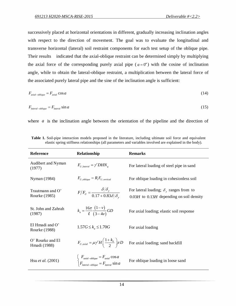
elastoplastic idealizations of the true nonlinear soil response. Table 1 summarizes the soil-pipe

interaction models presented next.

One of the first known such tests was conducted by Audibert and Nyman [23], who studied

the lateral (horizontal) response of steel pipelines buried in sand under a wide range of burial

depth to pipe diameter ratios and developed a rectangular hyberbola for modelling the soil

resistance as a function of the relative lateral movement. Their proposed ultimate soil resistance

against lateral pipe motion is given by:

,U lateral qF DHN (5)

where is the effective unit weight of the soil, D is the outside pipe diameter, H is the depth

to the pipe centreline and qN is the bearing capacity factor, estimated from appropriate charts.

Later, Nyman [24] investigated the restraints induced in cohesionless soil due to oblique

vertical-horizontal pipe motion. Extending the solution of Meyerhof [R] for inclined strip anchor

resistance, he proposed an expression for the ultimate soil restraint against the oblique pipe

motion as the product of the ultimate soil restraint against vertical pipe motion U,verticalF and an

inclination factor iR :

, ,U oblique i U verticalF R F (6)

with ,

,

0.251 1

90 0.75

U lateral

i

U vertical

FaR

a F

(7)

where a is defined as the inclination angle in degrees between the oblique and the vertical soil

restraint and U,lateralF can be evaluated from (5) or other sources. To completely describe the


12

nonlinear force-displacement relationship, Nyman recommends the following values for the

yield displacement of the soil that is required to mobilize the oblique ultimate soil restraint:

,

0.015

0.025y oblique

H for dense geomaterials

H for loose geomaterials

(8)

To validate the available analytical models against experimental data, Trautmann and O’

Rourke [25] performed a series of multi-parametric lateral loading tests to assess the response of

subsurface, typical-sized pipelines to lateral soil motion. A hyperbolic function was derived to

represent the average lateral force-displacement curve of the obtained test data, expressed in

dimensionless form as:

0.17 0.83

y

U

y

F F

(9)

where U hF HDLN is the ultimate soil force, with L and hN standing for the length and the

horizontal force factor, respectively. Appropriate values for the latter parameter may be sought in

relevant charts as a function of depth-to-diameter ratio and friction angle. Test results also

indicated a strong variation of the yield displacement y of the soil with the soil density, ranging

from 0.13H for loose soil to 0.08H for medium soil to 0.03H for dense soil.

In order to characterize the transverse horizontal and axial soil movement described in Eqs.

(3) and (4), St. John and Zahrah [20] used a foundation modulus obtained by manipulating the

solution to the Kelvin’s problem of a point static load applied within an infinite, homogeneous,

elastic, isotropic medium. The result was expressed as:

116

3 4a

vk GD

v

(10)

where v , G are the Poisson’s ratio and shear modulus of the medium and D the outer pipe

diameter. In the same manner, but utilizing the solution to the Flamant’s problem, they arrived at

an estimate for the foundation modulus that governs the pipe response to transverse vertical soil

motion:


13

2

1v

G Dk

v

(11)

Concerned with the evaluation of axial soil springs, El Hmadi and O’ Rourke [26] attempted

to verify the theoretical and empirical predictions for the axial spring stiffness available at that

time, taking advantage of the experimental data provided by a previous full-scale field test [27].

After performing a back-calculation on the governing displacement functions and also

considering the strain-dependent nature of the soil shear modulus, they ended up with an upper

and lower bound value for the axial spring constant ak as a function of the soil shear modulus G

:

1.57 1.70aG k G (12)

This range of values apparently lies within and consequently partly confirms the wider range

provided by the then existing literature 3aG k G . Another important finding of this study is

that the inertial axial force induced in the pipeline during the test was over two orders of

magnitude lower than the soil restraint developed, thus verifying the statement that pipeline

inertia is insignificant.

O’ Rourke and El Hmadi [15] established among others a relationship for the maximum

frictional resistance per unit length that develops at the soil-pipe interface under relative axial

motion between the soil and a pipeline with sand backfilling, considering that by definition this

is given by the product of the applied vertical force and the coefficient of friction. It may be

estimated as follows:

0,

1

2U axial

kF H D

(13)

where represents the coefficient of friction, 0k is the coefficient of lateral earth pressure and

D the circumference of the pipe.

In a later experimental effort, Hsu et al. [28] dealt with the response of pipes buried in loose

sand and subjected to oblique-horizontal increasing displacement. In specific, a large-scale test

was carried out involving various pipe specimens and depth configuration, wherein the pipe was


14

successively placed at horizontal orientations in different, gradually increasing inclination angles

with respect to the direction of movement. The goal was to evaluate the longitudinal and

transverse horizontal (lateral) soil restraint components for each test setup of the oblique pipe.

Their results indicated that the axial-oblique restraint can be determined simply by multiplying

the axial force of the corresponding purely axial pipe ( 0a ) with the cosine of inclination

angle, while to obtain the lateral-oblique restraint, a multiplication between the lateral force of

the associated purely lateral pipe and the sine of the inclination angle is sufficient:

cosaxial oblique axialF F a (14)

sinlateral oblique lateralF F a (15)

where a is the inclination angle between the orientation of the pipeline and the direction of

Table 1. Soil-pipe interaction models proposed in the literature, including ultimate soil force and equivalent

elastic spring stiffness relationships (all parameters and variables involved are explained in the body).

Reference Relationship Remarks

Audibert and Nyman

(1977) ,U lateral qF DHN For lateral loading of steel pipe in sand

Nyman (1984) , ,U oblique i U verticalF R F For oblique loading in cohesionless soil

Trautmann and O’

Rourke (1985) 0.17 0.83

y

U

y

F F

For lateral loading; y ranges from to

0.03H to 0.13H depending on soil density

St. John and Zahrah

(1987)

116

3 4a

vk GD

v

For axial loading; elastic soil response

El Hmadi and O’

Rourke (1988) 1.57 1.70aG k G For axial loading

O’ Rourke and El

Hmadi (1988) 0

,

1

2U axial

kF H D

For axial loading; sand backfill

Hsu et al. (2001) cos

sin

axial oblique axial

lateral oblique lateral

F F a

F F a

For oblique loading in loose sand


15

movement.

The American Lifeline Alliance presented a report [29] that contains mathematical

expressions for describing the behaviour of nonlinear soil springs in each of the four principal

directions of pipe motion, i.e. axial, lateral, vertical uplift and vertical bearing. In all cases, the

nonlinearity of the soil is idealized by an elastoplastic bilinear curve, hence only one point is

actually needed to define each curve. These models provide a way to estimate both the maximum

soil restraints and the corresponding relative displacements. The relationships (Table 2),

extensively used in design practice, were derived assuming uniform soil conditions and are

mainly based on Refs. [30,31]. Nourzadeh and Takada [7] use these relationships to generate soil

spring models in their numerical parametric investigation of the response of buried steel gas

pipelines to seismic wave propagation. Beam elements are used to model the pipeline and three-

component displacement time histories are used as seismic input. Analyses show that pipelines

experienced at least local buckling under PGAs greater than 0.6g; however, performance criteria

are too loosely defined to allow safe judgment.

Further, a number of recent studies have explored through analytical or numerical approaches

the response of buried steel pipelines to various types of tectonic fault movements, considering

the soil-pipe interaction. Karamitros et al. [32], extending the work by Kennedy et al. [R],

Table 2. Ultimate soil force and relative displacement relationships for soil-pipe relative motion proposed by

the ALA [29].

Spring direction Ultimate soil restraint Ultimate relative displacement

Axial 01

2

kDac H D

3 10mm depending onsoil stiffness

Lateral ch qhcDN DHN 0.04 2 0.10 ~ 0.15H D D D

Vertical uplift cv qvcDN DHN 0.01 ~ 0.02 0.1

0.1 ~ 0.2 0.2

H H D densetoloose sands

H H D stiff to soft clays

Vertical bearing 2

2c qb

DcDN DHN N

0.1

0.2

D for granular soils

D for cohesive soils

a : adhesion factor; c : backfill soil cohesion; chN , qhN , cvN , qvN , qbN , cN , N : bearing capacity factors in the

horizontal, vertical uplift and vertical bearing direction (subscripts c denotes clay, q denotes sand)


16

developed an analytical design methodology to estimate pipeline axial and bending strains

generated by strike-slip fault movement. In a series of studies [33,34], Vazouras et al. used

rigorous shell and solid finite elements for the soil-pipe model to study numerically the nonlinear

behaviour of buried steel pipelines crossing obliquely active strike-slip faults, also considering

the influence of pipe continuity by deriving special spring relationships for the model ends.

Sarvanis et al. [35] proceeded to build advanced finite element models for the soil-pipe

interaction problem in the axial and transverse direction by calibrating the involved parameters

through full-scale tests. Analysis of the calibrated numerical model under fault movement was

performed and results were compared to full-scale fault experiments, showing good agreement in

terms of axial strains. From a different perspective, Karamanos [36] points out that pipe elbows

exhibit more flexible behaviour compared to straight pipe parts and are more prone to section

ovalization due to bending and fatigue damage under cyclic loading. These facts render pipe

elbows the most critical components in a pipeline.

Remarks

A common deficiency in the majority of the cited studies (with few exceptions, see [37]) is that

the potential role of the kinematic part of interaction in the seismic response of the pipe is not

examined at all. More importantly, experimental studies dealing with the derivation of force-

deformation relationships for the soil springs are usually based on static loading tests, hence they

are most applicable to cases of earthquake-induced PGD. This, however, contradicts with the

true, cyclic nature of seismic excitation; hysterisis characteristics of both the pipe and the soil are

neglected. In view of this, emphasis should be placed on the development of reliable cyclic

force-displacement curves that describe the dynamic interaction between pipe and soil under

seismic shaking. Another assumption often used is the homogeneity of the medium along the

pipeline route, which apparently does not hold true considering that pipelines are geographically

distributed systems. Different lateral soil conditions might significantly affect the stress

distribution in the pipeline, as already indicated in some studies (e.g. [21,38,39]). This issue

requires further investigation in the framework of full dynamic soil-pipe interaction analysis

under the assumption of horizontally varying soil composition.


17

3 Predicting spatially variable transient ground motions along the pipeline

Spatial variability in earthquake ground motion can be interpreted as the differences expected in

frequency content, amplitude and phase angle of seismic signals captured at distant stations on a

local scale; this observation was consolidated over three decades ago, when researchers [40][41]

started analyzing the ample accelerogram data obtained from densely installed strong motion

recording arrays, in particular the SMART-1 array in Taiwan. Spatial variability is a physical

phenomenon of stochastic nature, in the sense that its occurrence can only be predicted with a

degree of uncertainty due to the complex, multi-parametric underlying mechanisms that

contribute to its generation.

These variations in the seismic ground motion are principally attributed to three factors [42]:

(a) the transmission of the waves at finite velocity (also known as the wave passage effect),

which intuitively results in different arrival times at different recording stations, (b) the gradual

reduction in the coherency of the waves as a result of successive scattering, such as reflections

and refractions, that occurs along their path through the non-homogenous earth strata (ray-path

effect) and due to the varying superposition of waves originating from different points of an

extended seismic source (extended source effect), collectively known as the ‘incoherence effect’,

(c) the different local soil conditions at remote stations that primarily affect the amplitude and

frequency content of the incoming waves (local site effect). Additional causes of the

phenomenon have also been recognized: the attenuation of seismic waves along their path,

resulting from the gradual dissipation of wave energy into the soil medium, and the relative

flexibility of the soil-foundation system that may ‘filter’ certain frequencies of the incoming

wave field [43]. However, the influence of the latter two sources is usually ignored in modeling

spatial variation of seismic ground motion as it is generally regarded insignificant.

Spatial variability in ground motion has been rigorously investigated by modeling the

earthquake ground acceleration as a random signal of time. Descriptors of the probabilistic

properties of the ground motions have been established and used to reflect the sources of spatial

variability [44]. Random vibration analysis or deterministic time-history analysis using simulated

spatially variable ground motions as input are employed to assess the effect of the phenomenon

on the response of various structures.


18

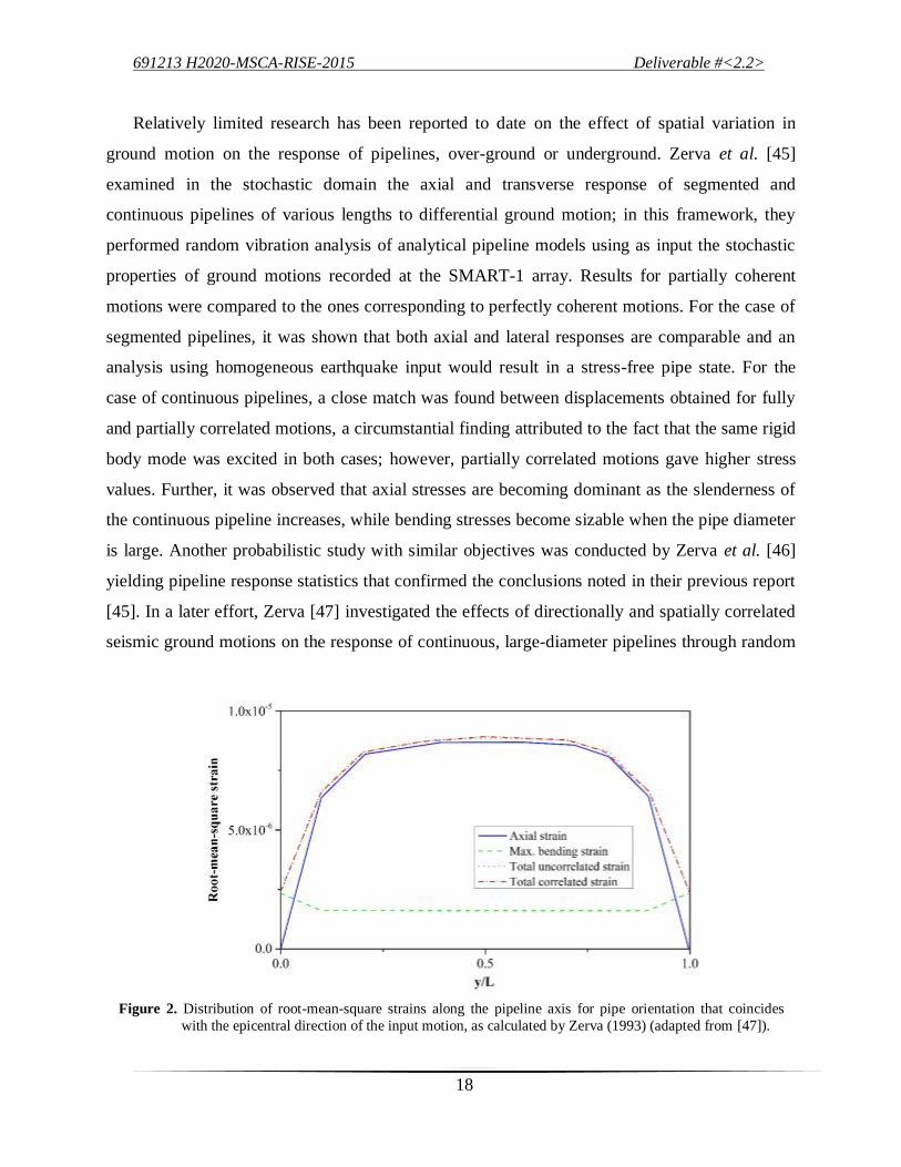
Relatively limited research has been reported to date on the effect of spatial variation in

ground motion on the response of pipelines, over-ground or underground. Zerva et al. [45]

examined in the stochastic domain the axial and transverse response of segmented and

continuous pipelines of various lengths to differential ground motion; in this framework, they

performed random vibration analysis of analytical pipeline models using as input the stochastic

properties of ground motions recorded at the SMART-1 array. Results for partially coherent

motions were compared to the ones corresponding to perfectly coherent motions. For the case of

segmented pipelines, it was shown that both axial and lateral responses are comparable and an

analysis using homogeneous earthquake input would result in a stress-free pipe state. For the

case of continuous pipelines, a close match was found between displacements obtained for fully

and partially correlated motions, a circumstantial finding attributed to the fact that the same rigid

body mode was excited in both cases; however, partially correlated motions gave higher stress

values. Further, it was observed that axial stresses are becoming dominant as the slenderness of

the continuous pipeline increases, while bending stresses become sizable when the pipe diameter

is large. Another probabilistic study with similar objectives was conducted by Zerva et al. [46]

yielding pipeline response statistics that confirmed the conclusions noted in their previous report

[45]. In a later effort, Zerva [47] investigated the effects of directionally and spatially correlated

seismic ground motions on the response of continuous, large-diameter pipelines through random

Figure 2. Distribution of root-mean-square strains along the pipeline axis for pipe orientation that coincides

with the epicentral direction of the input motion, as calculated by Zerva (1993) (adapted from [47]).


19

vibration analyses using similar analytical formulations as before and seismic input represented

by stochastic characteristics recorded at the SMART-1 array. The scrutiny revealed that

considering the correlation between the two horizontal seismic motion components provides

negligible discrepancies and that axial strains are the principal source of pipeline deformation

over bending strains (Figure 2); it was also shown that the selection of the incoherence

parameter on the pipeline response is critical (Figure 3).

Zerva [48] dealt with the effect of differential ground motions on the response of various

lifeline structures, including underground pipelines. By approximately estimating the seismic

axial strains along a buried pipeline model using two coherency decay models ([49], [50]), she

noted that these obtain their maximum values when the motions are totally incoherent, i.e. the

differential displacements at the input stations are maximum. Specifically for the second

coherency model, she observed an increasing trend in the seismic strains with increasing value of

the decay parameter a (denoting increasing incoherence). To further support the significance of

the incoherence effect, Zerva performed a comparative study to determine its relative influence

with respect to the wave passage effect. It was found that in the case of high apparent wave

propagation velocity, seismic strains along the pipeline are primarily controlled by the degree of

incoherence of the motions. On the other hand, for relatively lower values of apparent

propagation velocity, seismic strains are proportional to the reciprocal of this velocity. The study

Figure 3. Distribution of root-mean-square axial strains along the pipeline for different values of the

incoherence parameter, as calculated by Zerva (1993) (adapted from [47]).


20

by Lee et al. [51] uses multiple seismic excitation along a BNWF model of a pipeline in a 3D

nonlinear time-history analysis, showing that the pipeline presents varying distribution of the

axial relative displacement along its length, with peaks appearing in the region of differing

imposed excitations. As regards the transverse response, calculated pipeline demand for a

specific input ground motion reached half the respective capacity. It is also underlined that

transverse response under multiple excitation is affected by soil conditions.

Notwithstanding these pioneer previous studies, the conclusions drawn cannot be generalized

to describe the seismic response of buried pipelines to spatially variable ground motion, mainly

for three reasons. First, the results are plausibly specific to the recorded ground motion stochastic

characteristics selected for input. Second, the response of the pipeline depends highly on the

coherency model used in the analysis, which in turn has dependence on various incoherence

parameters. Third, the investigation so far is constrained in theoretical boundaries; further

evidence through laboratory work is deemed necessary in order to assess the degree to which

buried pipeline networks are vulnerable to differential seismic ground motions, especially

considering potential heterogeneities in soil conditions (local site effects), towards the

verification of the existing theoretical and numerical findings.

4 Dominant failure modes and supporting evidence from past earthquakes

In the course of earthquake-resistant design of underground pipeline networks, the principal

mechanisms that lead to failure due to seismic excitation have to be identified in order for

appropriate performance criteria to be established. Extensive previous research efforts and field

surveys have been successful in identifying the most frequently occurring failure modes,

classified into two groups: those observed in continuous and those observed in segmented

pipelines. The first group includes pipelines assembled with welded connections equally strong

or stronger than the pipe barrels, while the second group includes pipelines in which mechanical

joints are the weak link of the chain due to their lower strength. Herein, discussion is focused on

continuous pipelines. Assuming a flawless welding process and corrosion-free conditions, one

can distinguish five failure mechanisms for continuous steel-welded pipelines triggered by

ground shaking or PGD: pure tensile rupture, local bucking, upheaval buckling, flexural failure

and section distortion [52,53] (see Figure 4).


21

Tensile fracture

When excessive plastic longitudinal strains accumulate in pipe walls, rupture is expected to

occur. This type of failure is rarely observed in arc-welded steel pipelines with butt connections,

as these exhibit a strongly ductile behaviour. On the contrary, steel pipelines assembled with gas-

welded slip joints are more vulnerable to this failure mechanism, since they are incapable of

withstanding that substantial yielding before tensile rupture. This exact finding is concluded in

[54], based on relevant evidence from the 1994 Northridge event.

Although the fracture strain of X-grade pipe steel may well reach 6% [55], usually a more

conservative value of 3% [16,56] or 4% [52] is adopted in engineering practice. In general,

experience from previous earthquake events has shown that most steel pipelines exposed to

tensile loading performed more than sufficiently, since modern manufacturing techniques are

able to satisfy ductility requirements.

Local buckling

Local buckling (or shell wrinkling) is a failure state associated with structural instability issues

appearing under pipe compression. In essence, it involves localized distortion of the pipe wall,

which in turn can lead to further curvature amplification in that region and tearing. Local

buckling is a common failure mode in steel pipelines, as indicated by observations of pipeline

performance in past earthquakes [52]. Specifically, local buckling caused by wave propagation

Figure 4. Frequently observed failure mechanisms in buried continuous steel pipelines: (a) local buckling; (b)

tensile fracture; (c) upheaval buckling; (d) cross-section distortion


22

affected a water pipe during the 1985 Michoacan event in Mexico City, whilst liquid fuel, water

and gas pipelines were found to suffer such damage as a result of PGD in the 1991 Costa Rica

and 1994 Northridge earthquakes. More than that, local buckling due to PGD was evident in

pipelines crossing faults, both normal and reverse, in the 1971 San Fernando event. Experience

so far shows that local buckling distortions tend to accumulate at geometry transition regions of

the pipeline, such as bends and elbows.

Hall and Newmark [57], based on previous experimental results, recommended a failure

criterion for pipe local buckling by determining a range in which lies the critical compressive

strain corresponding to the onset of shell wrinkling. Later, this criterion was adopted as a design

provision by ASCE [58]. The range is expressed as:

0.30 0.40crt D t D (16)

where cr is the critical compressive strain marking the start of buckling, t and D are the wall

thickness and the outer diameter of the pipe, respectively. O’Rourke and Liu [52] note that the

above criterion finds better applicability to thin-walled pipes, while it is rather conservative for

thick-walled ones. Vazouras et al. [33] also establish a ‘no-buckling’ requirement for buried

pipelines deformed by strike-slip fault movement normal to their axis. After deriving a simplified

expression for the peak compressive pipe strain based on the assumption of a fixed deformed

shape and adopting a general form for the critical buckling strain as a function of the thickness-

to-diameter ratio, they arrived at the following limit condition:

2

0.4D t a L D (17)

where L is the length of the deformed segment of the pipeline and a is a parameter depending

on the pipeline material and initial imperfections.

Upheaval buckling

Steel pipelines subject to compressive ground forces are also likely to suffer from upheaval

(sometimes referred to as beam) buckling, a failure mode that resembles the well-known Euler

buckling of a column. In this failure mechanism, compressive strains are not confined in short

zones of the pipe walls, as in local buckling, rather they are distributed over greater lengths, at a

global level. For this reason, the likelihood of pipe breakage is generally lower than in the case


23

of local buckling, therefore upheaval buckling is a less catastrophic type of failure [52]. That

said, upheaval buckling is better characterized as a serviceability peril and not as a classic

material-related failure, since the pipeline can continue transmitting its contents along its extent.

On this basis, a criterion describing the limit state of a pipeline just before upheaval buckling

occurs is dependent on several parameters, such as the flexural rigidity of the pipe section,

potential structural imperfections and the burial depth of the pipeline, and consequently is

difficult to develop.

Meyersohn and O’Rourke [59] noticed that pipelines covered by backfill soil with limited

uplift resistance are more likely to fail by means of upheaval buckling. They pointed out that

there is a proportional relationship between buckling load and trench depth and calculated a

critical value for the latter, which in effect determines the precedence of occurrence of the two

modes of buckling; that is, if a pipeline has a larger burial depth than the critical cover depth,

then local buckling will occur before upheaval buckling and vice versa. Further on this, it was

noted that a minimum cover depth of 0.5 to 1.0 m is sufficient to ensure that the pipeline will not

experience upheaval buckling.

Observations from previous earthquakes reveal that upheaval buckling has indeed affected

underground pipelines in some cases. In 1959, oil pipelines covered with a shallow trench with a

depth ranging between 0.15 and 0.30 m and traversing the Buena Vista reverse fault lifted out of

the ground because of high compressional stresses. In another interesting occasion related to the

1979 Imperial Valley seismic event, no evidence of upheaval buckling in two pipelines crossing

the fault was available until local inspections by means of cover removal forced the pipelines to

buckle upwards [60]. This is also an indication that upheaval buckling may not always interrupt

the functionality of the pipeline.

Flexural failure

Failure due to excessive bending of the pipe section is quite rare in steel pipelines because of the

high ductility of steel. To this conclusion points among others evidence from the 1971 San

Fernando earthquake event, where a number of buried gas and liquid fuel pipelines were found to

have endured approximately 2.5 m of transverse soil displacement [61].

Section distortion


24

Another possible failure associated with large radial deformations is the cross-sectional

distortion or ‘ovalization’, as is the term most frequently used. Severe bending may force the

pipe circular cross-section to flatten into an oval-like shape, which can pose a serviceability

threat to the pipeline carrying capacity. The limit state for this failure mode has been codified by

Gresnigt [62] through a critical change in the pipe diameter crD as:

0.15crD D (18)

It is important to emphasize that a different approach to the establishment of failure criteria is

expected to be followed for continuous pipelines with slip, riveted or gas-welded joints. As

opposed to pipelines assembled with butt joints, for which failure criteria are mostly functions of

pipe performance indicators, in this case failure criteria have to be formulated on the basis of

joint characteristics, because this type of joints are generally weaker than the main pipe body. A

number of studies involved the estimation of the strength of slip joints with inner [63,64] and

outer weld [65] in terms of joint efficiency, namely the ratio of joint to pipe strength. Joint

efficiency values lower than 0.40 were obtained in all cases. Damage evidence at welded joints is

available from the 1971 San Fernando earthquake, where most of the failures were observed at

the welds of gas-welded joints.

Recent damage observations and remarks

Damage in buried pipelines caused by recent major earthquakes is a subject of current scrutiny.

Esposito et al. [66] recorded a significant level of damage in gas-welded steel joints in the local

underground gas distribution network after the 2009 L’Aquila event. This damage is described as

breaks or leaks, but no further details as to the exact failure modes are provided. Koike et al.

[67], in estimating the seismic performance of the gas pipeline network following the devastating

2011 Tohoku event in Japan, note that high-pressure transmission pipelines survived successfully

the impact of the earthquake with only minor damage, even in mountain settings where

landslides occurred. More recently, Edkins et al. [68] identified the characteristic failure

mechanisms affecting buried pipelines of different materials, based on interpretation of

photographic material obtained after the 2010/2011 Canterbury earthquakes. They conclude that

different failure modes may occur depending on the material, the soil conditions, direction of

excitation and pipeline size. The samples examined do not include any steel pipelines, though.


25

Focusing attention on steel pipelines, which typically make up for the largest part of gas

transmission networks, it becomes clear that the existing failure criteria lack robust scientific

basis. Physical testing of specimens under controlled laboratory conditions is necessary in order

to determine limit state parameters governing different failure modes and also clarify the

influence of factors such as soil conditions and pipeline size. Furthermore, when performing

numerical investigations, emphasis should be placed on the selection of the finite element model;

failure states like local buckling and section deformation cannot be predicted by simple beam

models, as this requires the adoption of more sophisticated cylindrical shell models.

5 Fragility expressions for buried pipelines

In the last decades, a gradual transition is seen in the interest of the structural engineering

community from conventional deterministic analysis procedures to probabilistic risk assessment

concepts, as the understanding of how various uncertainty sources, both aleatory and epistemic,

may affect the basic variables governing the response of structures to natural hazards is

becoming more profound and the available computational capabilities are rapidly evolving.

Particularly in earthquake engineering problems, wherein uncertainties due to the nature of the

hazard are amplified, structural reliability tools have drawn significant research attention lately

in an attempt to quantify these uncertainties, explore their potential propagation throughout the

model and evaluate the risk level the structure is exposed to. When it comes to the seismic safety

of infrastructure of paramount civil importance, such as utility systems, probabilistic approaches

are deemed more than necessary to secure minimum functionality disruption and overall

longevity under different excitation levels.

In a broad context, a fragility curve expresses the conditional probability that a structural

system or individual component of the system reaches or exceeds a certain limit damage state for

a given load intensity. This probability measure is commonly referred to as the probability of

failure, where the term ‘failure’ does not necessarily imply catastrophic damage, rather refers to

different predefined levels of so-called unsatisfactory performance. In the sphere of earthquake

engineering, fragility curves are used to investigate the probability that the imposed seismic

demand D is equal to or greater than the capacity C corresponding to a specified damage state

of the structure, given a ground motion intensity measure ( IM hereafter) magnitude, according

to the following probability statement:


26

|Fragility P D C IM (19)

In the context of damage analysis of buried pipelines, probabilistic expressions known as

seismic fragility relations are the typically used evaluation tool. They establish a relationship

between the spatially distributed pipe damage rates and the different degrees of earthquake

severity. The damage rate is usually quantified as the pipeline repair rate, i.e. the number of pipe

repairs (breaks or leaks) per unit length of pipelines, although other measures have also been

used. Seismic fragility relations are usually categorized according to the damage source, that is,

TGD and PGD, and are written as:

bRR aIM (20)

where RR is the median repair rate and a and b are parameters estimated from regression

analysis of the available data pairs.

Several different ground motion IMs have been claimed in the literature to correlate well

with pipeline damage, ranging from the generally adopted MMI, PGA, PGV, AI, 1aS T to the

more pipeline-specific peak ground strain g and 2 /PGV PGA . The majority of studies on

seismic fragility of buried pipelines adhere to the fragility relation scheme based on collected

empirical data. At least to the authors’ knowledge, only few research efforts [69,70] have

advanced to producing classic fragility curves by calculating probabilities of failure.

Empirical seismic fragility relations for buried pipelines

The first studies that utilized observed pipe damage from earthquakes date back to 1975, when

Katayama et al. [71] published charts of pipe damage as a function of PGA for different soil

categories, taking into account data obtained from six events. Later, Eguchi [72] generated

expressions for pipe breaks in terms of the MMI scale for various pipe materials, being the first

to distinguish between wave propagation and PGD hazards and providing a ranking in terms of

vulnerability of different pipe materials as follows (in descending order): concrete, PVC, cast

iron, ductile iron, X-grade steel. Barenberg [73] and Ballantyne et al. [74] first developed

fragility relations considering PGV as the ground motion IM. Along the same lines, empirical

PGA-based fragility expressions were produced in three subsequent studies [75–77].


27

A remarkable effort in the literature is that of M. J. O’ Rourke and Ayala [78], who proposed

a PGV-based seismic fragility relation based on damage data associated with pipelines of various

materials from three earthquake events. Their function concerning damage due to wave

propagation was adopted by FEMA in HAZUS methodology [79]. Further on this subject, T. D.

O’Rourke et al. [80] performed comparative damage analyses using different IMs; their

conclusion was that the highest correlation between damage and seismic severity is achieved

with the use of PGV as IM. In an alternative approach, Trifunac and Todorovska [81] defined the

damage rate as the amount of pipe breaks per square km of land area and used the peak soil shear

strain as IM to derive fragility expressions for water pipelines based on the 1994 Northridge

event. T. D. O’Rourke and Jeon [82] used cast iron pipe damage evidence from the 1994

Northridge event to develop a fragility relation for wave propagation.

In a relevant guideline document [83], the American Lifeline Alliance incorporated the most

comprehensive list of seismic fragility relations for water supply pipelines, based on an extensive

database of documented damage that includes 81 data points. The relations are provided in the

form of backbone functions, allowing for adjustment through correction factors to account for

different pipe materials, joint types and other parameters, and their validity has been confirmed

in practice in recent earthquake events. It should be noted that the damage data present

considerable scatter and, moreover, refer mostly to cast iron and asbestos cement pipeline. In

another notable publication, M. J. O’ Rourke and Deyoe [84] accomplished a twofold objective,

re-examining previously used data sets related to segmented buried pipes: on the one hand to

illustrate that the peak ground strain g is more consistent than PGV in describing seismic

damage to segmented buried pipes, on the other hand to develop improved fragility relations in

terms of g and also PGV-based relations considering the type of the controlling seismic wave.

These relations are based on the assumption that S-waves govern for near-source sites and R-

waves for far-source sites. Jeon and T. D. O’Rourke [85] performed comparisons among damage

prediction equations using differently estimated PGV, concluding that the maximum recorded

PGV value provides better correlation with water supply pipeline damage rates. Later, Pineda

and Ordaz [86] proposed a new IM for buried pipeline fragility functions, 2 /PGV PGA , and

showed that it is more closely related to damage patterns in soft soils. By assuming different


28

effective wave velocity, M. J. O’ Rourke [87] presented a revised strain-based fragility relation

for segmented pipes exposed to seismic wave propagation.

Esposito et al. [66] presented a comprehensive study analyzing the performance of the

L’Aquila medium- and low-pressure gas distribution network in the 2009 earthquake. Relying on

damage reports, seismic fragility of buried steel pipes in terms of repair rates was estimated and

plotted against local-scale PGV values interpolated using Shakemap tools. Then, the obtained

data were validated against existing fragility relations, giving non-negligible damage

underestimations by the latter. The deviations were attributed to the fact that the fragility

relations used were established for arc-welded steel pipes, while the L’Aquila gas pipeline

network consists of gas-welded pipes, which are more vulnerable. Noteworthy is the fact that

HDPE pipes exhibited no damage at all. More recently, T. D. O’Rourke et al. [88] assessed the

performance of underground water, wastewater and gas pipelines during the 2011 Canterbury

seismic episodes. By processing vast amounts of damage data through screening criteria, they

developed robust fragility relations for different pipe materials, using geometric mean PGV,

angular distortion and lateral peak ground strain as IMs. Specifically for the gas distribution

network performance, they comment that it remained almost undamaged, owing to the good

Figure 5. Comparative log-scale plot of published strain-based empirical fragility relations for buried pipelines.


29

ductility of MDPE pipelines. Further, M. J. O’ Rourke et al. [89] enriched the fragility relation

proposed by M. J. O’ Rourke [87] with four additional data points obtained from the 1999

Kocaeli event. This fragility relation does not differ significantly from the initial one, hence

demonstrating that the latter is fairly stable. All strain-based fragility relations are plotted in

Figure 5; all empirical fragility expressions cited herein are summarized in Table 3.

Lanzano et al. [69] published one of the few studies that addresses complete fragility curves,

Table 3. Summary of the most recent empirical fragility functions in terms of repair rate (RR/km) for buried

pipelines found in the literature; PGV in cm/s, 1K and

2K : correction factors that apply to certain

pipe types, PGD in cm, g : peak ground strain, GMPGV : geometric mean PGV

Reference Fragility function Remarks

M. J. O’ Rourke and Ayala (1989) 2.67

50PGV Wave propagation damage

T. D. O’Rourke and Jeon (1999) 1.220.00109 PGV Wave propagation damage, CI pipes

ALA (2001) 1 0.002416K PGV Wave propagation damage, various

pipe typologies

ALA (2001) 0.319

2 2.5831K PGD PGD damage, various pipe typologies

M. J. O’ Rourke and Deyoe (2004) 0.89513 g Wave propagation damage, segmented

pipes

M. J. O’ Rourke and Deyoe (2004) 0.92724 g Combined wave propagation and PGD

damage, segmented pipes

M. J. O’ Rourke and Deyoe (2004) 0.920.034 PGV Wave propagation damage, surface

waves

M. J. O’ Rourke and Deyoe (2004) 0.920.0035 PGV Wave propagation damage, body waves

M. J. O’ Rourke (2009a) 1.121905 g Wave propagation damage, segmented

pipes

T. D. O’Rourke et al. (2014) 4.52 2.3810 GMPGV Wave propagation damage, CI pipes

T. D. O’Rourke et al. (2014) 0.0839 0.41g Lateral ground strain damage, CI pipes

M. J. O’ Rourke et al. (2015) 1.162951 g Wave propagation damage, segmented

pipes


30

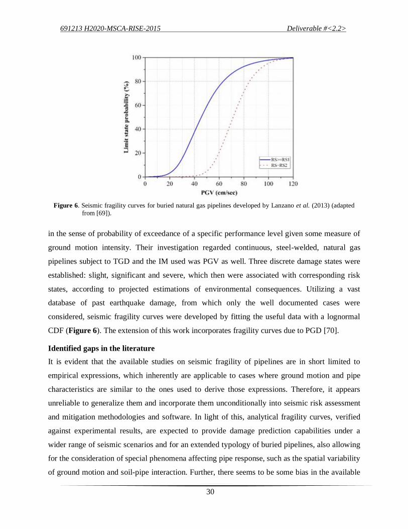
in the sense of probability of exceedance of a specific performance level given some measure of

ground motion intensity. Their investigation regarded continuous, steel-welded, natural gas

pipelines subject to TGD and the IM used was PGV as well. Three discrete damage states were

established: slight, significant and severe, which then were associated with corresponding risk

states, according to projected estimations of environmental consequences. Utilizing a vast

database of past earthquake damage, from which only the well documented cases were

considered, seismic fragility curves were developed by fitting the useful data with a lognormal

CDF (Figure 6). The extension of this work incorporates fragility curves due to PGD [70].

Identified gaps in the literature

It is evident that the available studies on seismic fragility of pipelines are in short limited to

empirical expressions, which inherently are applicable to cases where ground motion and pipe

characteristics are similar to the ones used to derive those expressions. Therefore, it appears

unreliable to generalize them and incorporate them unconditionally into seismic risk assessment

and mitigation methodologies and software. In light of this, analytical fragility curves, verified

against experimental results, are expected to provide damage prediction capabilities under a

wider range of seismic scenarios and for an extended typology of buried pipelines, also allowing

for the consideration of special phenomena affecting pipe response, such as the spatial variability

of ground motion and soil-pipe interaction. Further, there seems to be some bias in the available

Figure 6. Seismic fragility curves for buried natural gas pipelines developed by Lanzano et al. (2013) (adapted

from [69]).


31

damage information, as most of it concerns segmented water pipelines. Vulnerability research

addressing continuous steel pipelines with welded joints, which is usually the case in buried

natural gas pipelines, is scarce; hence, this issue remains to be illuminated.

6 Pipeline health monitoring for maintenance and rehabilitation

The demand by society imposed on the engineering community for sustainable infrastructure is

constantly growing. To achieve the goal of sustainability, two major requirements must be met

during the design life of an infrastructure: regular maintenance and quick rehabilitation after an

extreme event. In this respect, an integral part of the desired service lifecycle of lifelines is the

implementation of non-destructive Structural Health Monitoring (SHM) methods during their

operation towards the reliable diagnosis of their structural condition. Several, yet not entirely

different definitions have been proposed for the arguably fast-evolving practice of SHM.

According to Chang [90], for instance, SHM provides the means to continuously gather (near)

real-time information on the integrity of infrastructure without interruption of their service, with

the final goal being hazard mitigation. Nevertheless, almost all definitions agree on some basic

aspects [91] that are typical of SHM applications, including:

(1) Almost real-time health screening

(2) No service interruption during the monitoring process

(3) Deployment of sensing instruments capturing on a continuous basis variations in specific

metrics that determine the state of the structure

(4) Transmission of acquired data through an established wired or wireless network

(5) Data analysis in order to detect damage patterns and assess damage modes and extent

SHM finds application on nearly every lifeline system and tends to become standard practice

nowadays, given their importance for the societal well-being; underground energy pipelines are

no exception to this. Past experience has shown that natural hazards such as earthquakes can

cause severe damage to buried natural gas pipelines, leading to content leakage, which in turn

may trigger explosions, fires and atmospheric pollution. On top of this, pipe deterioration may be

accelerated by previous time-dependent material degradation and ageing, or even manufacturing

defects. Therefore, it becomes clear that pipeline monitoring to track structural integrity over

time should be a matter of priority for natural gas pipeline operators in the framework of a long-

term management strategy that ultimately aims for life extension of the pipeline and minimum


32

supply interruption. Besides, the pipeline industry is bound to special regulations that require the

implementation of inspection procedures on existing pipelines [92]. Pipeline SHM techniques

can prove useful both (a) as a prevention tool, in that they can detect in-time accumulated

damage due to service loads, wearing and pre-existing flaws prior to any failure and (b) as a

remediation tool, in that they can rapidly localize and characterize incurred damage immediately

after the occurrence of an earthquake.

Scheduled maintenance by means of visual in situ inspections has now been replaced to a

great degree by cutting-edge techniques that not only offer a broader insight of the structure’s

integrity indicators both in space and in time, but also minimize labor and downtime costs.

Excluding the outdated and inefficient in situ inspection, three are currently the main sensing

technologies used in pipeline SHM [93]:

(a) in-line inspection techniques

(b) fiber optic sensing

(c) remote sensing

Of the three, the first two are the dominant trends in pipeline industry, and for this reason

emphasis herein will be placed on these.

In-line inspection techniques

Perhaps the most widely adopted approach in SHM of buried natural gas pipelines today is the

so-called in-line inspection. Essentially, small autonomous devices known as ‘smart pigs’ (the

term ‘pig’ derives from Pipeline Inspection Gauge) and carrying sensors, data recorders and

transmitters are inserted inside the pipeline and driven by content flow, ‘in-line’ with it. As they

travel long distances in the interior of the pipe, the mounted sensors obtain continuous

measurements of various parameters, depending on the desired inspection tasks; these are

typically related to geometry checks, strain analysis, metal loss and crack detection. In this

manner, large pipeline segments can be examined at reduced times without blocking the

transportation process of natural gas.

The basic principle behind the measuring activity that gives meaning to the obtained data is

that consecutive measurements are taken over time, thus any change with respect to previously

obtained values related to undamaged state will denote a health issue. After proper statistical


33

processing, these data are compared to measurements corresponding to the so-called ‘learning’

period and diagnosis is then made with respect to the integrity of the pipeline.

Commercially available in-line inspection tools are based on various sensing technologies

[93]. Among them, ultrasound-based sensors are common in the market for metal loss and crack

inspections. These are sensing transducers that emit ultrasonic pulses in the direction of the pipe

wall. The acoustic signals are then reflected from both the inner and the outer wall surface and

captured back from the transducer (Figure 7a). From the knowledge of the sound velocity in the

medium and by measuring the traveling times of the signal, wall thickness is computed and any

metal loss can be inferred. The transducers may be piezo-electric or electro-magnetic, with the

latter being the case for natural gas pipelines as the former require a liquid medium to function,

and may also be installed on the external surface of the pipeline. Another highly popular in-line

inspection technology tailored to corrosion detection of steel pipelines is magnetic flux leakage.

According to the underlying physical principle of magnetization, the inspection unit transmits

magnetic flux into the pipe-wall, creating a magnetic circuit. If metal corrosion is present in

certain regions, there will be some sort of leakage in the magnetic field, which is detected by

Figure 7. Schematic views of in-line inspection technologies: (a) Principle of ultra-sound based sensors

(reprinted from [92]; (b) Principle of magnetic flux leakage sensors


34

magnetic sensors placed on the unit (Figure 7b). Moreover, the latest industry trends suggest the

combined utilization of different sensing technologies on a single in-line inspection tool in order

to carry out more reliable, multi-purpose pipeline inspections.

Distributed fiber optic sensing

Fiber optic sensors are one of the most promising technological developments in the field of

SHM, although their first use can be traced back as early as the 1970s [93]. The function of fiber

optic systems is based on the physical properties of light propagation: the goal is to associate

unexpected variations in the light signals as they travel along fiber strands with damage patterns.

Through various configurations, fiber optic sensing offers diverse capabilities in measuring a

number of different parameters, including strain, temperature, pressure and acceleration [91].

What is of interest in examining the condition of a pipeline subject to earthquake effects is

primarily the strain levels in the pipeline. Discrete and, lately, distributed fiber optic sensors have

been used for strain monitoring purposes. Although discrete sensors provide unmatched

resolution and accuracy in local-scale measurements, they are not suitable for global monitoring,

as this would require the installation of thousands of them along the pipeline, together with a

complex wiring system, leading to prohibitively high costs.

This significant drawback is surmounted by the distributed fiber optic sensors, which are

capable of efficiently monitoring large portions of such elongated systems as pipelines.

Distributed sensors are fairly simple in their structure; they comprise a single silicon fiber cable

sensitive at its whole length, which is tightly bonded to the pipe wall upon installation in order to

allow lossless transfer of the material strains. Low attenuation levels ensure that distributed

sensors perform well over distances of up to 25 km [94]. Other advantages of the distributed

sensing technology include simple cable connections to the data receiver and reduced installation

effort and cost.

Distributed fiber sensing technology relies on one of the following three optical effects:

Rayleigh scattering [95], Raman scattering [96] and Brillouin scattering [97]. Technical details

about these fall out of the scope of this study and may be found in the relevant references.

Brillouin scattering-based implementations are usually the method of choice, since they suffer

the least from signal losses and they are capable of long-range monitoring [98]. Several

experimental studies have been conducted that demonstrate the effectiveness of the method. For


35

instance, Inaudi and Glisic [94] present the results of the field application of a previously

developed Brillouin distributed strain, temperature and combined strain-temperature sensing

instrument (DiTeSt) [99]. Excellent performance of distributed strain monitoring on a buried gas

pipeline subjected to landslide loading was reported, as well as successful detection of the

leakage spot by the distributed temperature sensors during a gas leakage simulation. In an earlier

laboratory test, Ravet et al. [100] took advantage of the unique capability of distributed Brillouin

sensors to measure both tension and compression at the same time, in order to detect the starting

point of buckling in a steel pipe under axial compressive load. To ensure prior knowledge of the

location of buckling initiation, weakening of the specimen wall was performed at a specific

region. Comparison between the measurements from the distributed Brillouin sensor and

installed strain gauges along the pipe body showed good agreement, and tensile strains were

successfully detected by the distributed Brillouin sensor, signifying the initiation of the buckling

process. Glisic and Yao [98] put extensive efforts in developing an integrated damage

monitoring method of buried concrete segmented pipelines exposed to seismic effects, using

distributed Brillouin scattering-based fiber optic sensors. In validating the method with large-

scale testing, PGD was simulated to act on a 13 m-long pipeline assembled inside a test basin

Figure 8. Select results from the pipe strain monitoring experiment with distributed Brillouin sensors conducted

by Glisic and Yao (2012), indicating detected damage (reprinted from [98])


36

and covered with soil, while strain readings obtained from the fiber optic sensors were verified

against data from conventional strain gauges (Figure 8). Damage accumulation in the joints was

mainly observed, as expected, and the sensing system achieved to identify these patterns as strain

peaks in the strain profiles. The applicability of the method can be safely extended to continuous

steel pipelines according to the authors.

Critical summary and issues to be addressed

The aforementioned pipeline inspection techniques are not universally applicable in industrial

practice, as they present specific drawbacks that limit their implementation. A crucial factor that

determines the suitability of in-line inspection tools is the potential of the pipeline to permit

passage of the pig unit through its body (known as ‘pigability’), which depends on a number of

pipeline attributes, such as the size of the pipe section, the operational pressure and the flow

conditions [101]. Besides, in-line inspection requires some degree of manual operation, as well

as efficient energy management of the wireless sensors. More importantly, in-line inspection

techniques are considered less suitable than distributed fiber optic sensing for emergency-state

rapid damage detection following an earthquake, as they require longer operating times. On the

other hand, fiber optic solutions are particularly expensive, and their cost tends to increase

dramatically with higher measurement accuracy. Distributed fiber sensors also require more

intricate installation procedures and ensuring of good bonding with the pipe wall is a prerequisite

for accurate sensor readings; further to this, optimized placement of the distributed sensors on

the pipe circumference is another concern for reliable integrity monitoring [102].

As general remarks concerning the full spectrum of available inspection technologies, it

should first be underlined that there is a general difficulty in handling effectively the vast amount

of data that are acquired from long-term pipeline monitoring facilities, and this may place doubts

on the credibility of the results. To this end, efforts should be put towards the development of

efficient data processing tools that incorporate sophisticated threshold-based algorithms of

deterministic or statistical background, in order to reliably interpret captured metrics variations

on the basis of previous samples. Second, the major challenge is to take advantage of the existing

pipeline SHM technologies in a holistic approach involving rapid post-rupture health assessment,

fast repair actions and decision-making in the direction of network resilience. Such

considerations should not ignore the fact that, during a post-earthquake crisis period, power


37

supply and wireless communications networks may experience long-lasting outages, hence

hindering any integrity assessment works.

7 The emerging concept of resilience in pipeline networks

Resilience is a recently developed and rapidly-accepted concept in the field of lifeline

engineering that can be understood in the context of emergency situations caused by natural (e.g.

earthquakes, floods, hurricanes) or man-made (e.g. vehicle collisions, bomb explosions) extreme

events that induce abrupt variations in the performance of lifelines. In engineering terms,

resilience denotes a highly desirable property referring to either physical (infrastructure) or social

(communities) systems that requires multidisciplinary considerations for its quantification (it

draws information from seismology, earthquake engineering, economics, social and management

sciences) and careful treatment to discern it from closely related concepts such as vulnerability,

fragility, risk and sustainability.

Analytical treatment of resilience


38

In a pioneer work, Bruneau et al. [103] set the foundations for the quantitative assessment of

seismic resilience. They define a resilient system as one that obeys to three basic rules:

• It is characterized by enhanced reliability.

• It generates tolerable levels of losses when experiencing failure.

• It is capable of returning quickly to a previous performance standard after failure.

The preliminary identification of these core features of resilience helps develop a

comprehensive mathematical definition of it. Drawing upon a study by Cimellaro et al. [104],

seismic resilience is an index R representing the capacity of an infrastructure system or

community to withstand earthquake effects by retaining an acceptable level of performance over

a given post-earthquake time period, through a process involving loss estimation, collection of

resources, relief strategy planning and restoration actions. The time-dependent performance of

the system is measured with functionality Q t , a dimensionless function of time denoting the

service quality of an infrastructure system at any time instant as a proportion of the full

Figure 9. Graphical illustration of time-variant functionality, resilience, rapidity and robustness; R : resilience;

avgr : average rapidity; RET : recovery time


39

functionality corresponding to the initial, intact state of the system, assumed to be equal to 100%

(Figure 9). Functionality can be modelled as a non-stationary stochastic process [104]. A

mathematical definition of seismic resilience under the consideration of a single seismic event is

possible:

00

1 ht

h t

R Q t dtt t

(21)

where 0t is the time of the occurrence of the seismic event and

ht is the investigated time

horizon. Graphically, Eq. (21) represents the shaded area underneath Q t over the time interval

0ht t , normalized with respect to this interval, as illustrated in Figure 9. The mathematical

definition of functionality involved in Eq. (21) may vary depending on the system examined.

Dimensions of resilience

While establishing a quantitative definition of resilience is difficult, evaluating it and finding

ways to enhance it pose a further challenge, given the various sources of uncertainty that arise

and the subjectivity of the problem. This task can be facilitated if the idea of resilience is broken

down into simpler descriptors, as Bruneau et al. [103] propose: (a) rapidity, (b) robustness, (c)

redundancy and (d) resourcefulness. Detailed descriptions of these quantities are available in

Refs. [103,105]. Rapidity and robustness are quantifiable (refer to Figure 9), while redundancy

and resourcefulness are more abstract qualities of an infrastructure system, difficult to quantify

and also interlinked with each other. To make a distinction from rapidity and robustness,

redundancy and resourcefulness provide the means to achieve resilience, whereas rapidity and

robustness are descriptors of the final outcome.

Bruneau et al. also introduce an alternative way to qualitatively characterize resilience

depending on its context. On this basis, they distinguish the technical, organizational, social and

economic dimension of resilience. As it becomes clear out of this classification, different

performance measures need to be employed for the quantification of these four dimensions,

varying from case to case. The first two dimensions of resilience are considered at the

facility/physical system level, while the latter two refer to the wider community spectrum.

Previous research on seismic resilience assessment of buried pipeline networks


40

Only a handful of studies on quantitative evaluation of seismic resilience are on record, since it is

a topic that has gained popularity lately. Esposito et al. [66], in assessing the impact of the 2009

L’Aquila earthquake on the local gas network performance, analyzed the over time network

functionality reinstatement described in terms of the ratio of reconnected customers over total

customers after the shock, showing that only 40% of the customers were reconnected to gas

supply after two months. This functionality evolution was compared to a hypothetical ideal one,

which however is not explained how it was estimated. The low restoration level achieved is

attributed to the fact that reconnection was permitted only to buildings that received a green-tag

during post-earthquake inspection.

More recently, Cimelarro et al. [106] developed and applied to a case study a comprehensive

quantitative framework for the seismic risk analysis of gas distribution networks considering the

impacted network functionality and the ensuing recovery process. Network functionality defined

as a function of the time-variant gas flow and total operating pipe length was computed with

numerical modeling using SynerGEE software. A single seismic scenario was extracted by de-

aggregating local hazard maps corresponding to 22% probability of exceedance in 50 years and

median PGV maps were calculated using attenuation relationships. Only PGD-induced pipe

damage was considered and fragility relations developed by ALA [83] were exploited to express

pipe damage distribution in a repair rate format. Then, 14 pipe breakage scenarios were defined

and localized within the network based on a Poisson probability model, bridge collapse

hypotheses and engineering judgment. The study ended with the estimation of resilience indices

of the gas network for all damage scenarios, before and after the application of a retrofit

alternative including emergency shutoff valves and flow dividers.

The need to extend and expand the seismic resilience assessment framework to buried

natural gas networks

Despite the valuable but scarce previous contributions, the relevant literature database is still

lacking an integrated risk assessment and management methodology for buried natural gas

networks that would address the involved aspects altogether: seismic hazard, seismic

vulnerability of individual network components, interdependence of network components,

overall network vulnerability and seismic losses and comparative evaluation of loss mitigation

strategies reflected on measured resilience levels, in a pre-earthquake probabilistic context and

under the consideration of the particularities of such a network, such as the weak flow


41

redistribution capabilities and the high fire likelihood due to gas escape. The development of

such methodology would assist engineers in accomplishing optimized network designs in terms

of resilience in earthquake-prone areas; it would also assist managerial groups in (a) decision-

making at a post-earthquake level aiming at limiting consequences and regaining initial network

functionality shortly and (b) in enhancing preparedness levels at a pre-earthquake level in order

to deliver the most effective emergency response in case of a future seismic event. So far, most

of the risk-related research has focused on loss assessment and loss reduction resulting from

different policies; however, a comprehensive seismic risk mitigation framework (and probably

software tool as well) centered at seismic resilience, as the one described herein, would expand

far beyond. Evident is also the lack of a robust and reliable functionality metric tailored to

natural gas networks, that would account for the dependency of other lifelines on the gas network

[107].

8 Current codes of practice and guidelines for earthquake-resistant design of

buried pipelines

Presently, only few modern norms worldwide dictate requirements for the protection of

underground natural gas pipelines against seismic risk, the most notable being Eurocode 8 - Part

4 [16] in the European Union, the American Lifeline Alliance guideline [29] in the US and the

design recommendations by Japan Gas Association [56]. In this section, the key points in each

normative document are discussed.

Eurocode 8 provisions (2006)

Part 4 of Eurocode 8 [16] provides a broad regulatory framework for the seismic design of

pipelines, inter alias. According to it, the ultimate limit state of a pipeline is associated with

structural collapse. Yet, it is implied that certain critical components of the system susceptible to

brittle failure may be checked for a state prior to total failure. A two-level serviceability limit

state hierarchy is prescribed; the lower one requires that the system remains fully operational and

leak-proof and the higher one that it undergoes some level of damage without losing its whole

supplying capacity. Another secondary safety hazard that should be taken into consideration in

ultimate limit state design is explosion and fire in the event of an earthquake-induced breakage

and the potential consequences on people and the environment. The determination of the seismic


42

actions should be based on the two principal sources of damage, i.e., seismic wave propagation

and PGD.

Further, Eurocode 8 states that pipe inertial forces related to ground acceleration are of minor

significance in comparison with the forces caused by ground deformation, thus they may be

neglected; this simplifies the nature of the problem, converting it to a static one. With regard to

wave propagation effects, Annex B of Eurocode 8 recommends the conservative method

developed by Newmark [17] to determine the induced pipe strains and curvatures, as long as the

soil is stable and homogeneous. As for the spatial variability in ground motion, no particular

guideline is provided; however, in the chapter concerning above-ground pipelines, it is suggested

that spatial variability is accounted for when the pipeline length analyzed is over 600 m or the

ground is characterized by longitudinal non-uniformities. It is also noted that pipelines buried in

dense soil are allowed to be designed solely for the effects of wave propagation.

When it comes to PGD, Eurocode 8 provides a set of specific design rules to improve

resistance. In the case that the pipeline route crosses an active fault zone, the design should in

general ensure maximum flexibility of the soil-pipe system, so that the pipeline can withstand

larger deformations. Pipelines crossing strike-slip or reverse faults should be oriented in such an

angle that the affected pipe segment is subjected predominantly to tension and not compression,

thus taking advantage of the available ductility of steel. Other site-specific construction measures

include minimizing the burial depth, increasing pipe wall thickness within a 50 m-zone on both

sides of the fault, using a hard and smooth pipe coating to reduce the angle of interface friction

between the pipe and the soil, using soft soil as backfill and avoiding significant deviations from

a straight line alignment. Annex B suggests that a simplified method to modeling the

phenomenon is to apply a relative static displacement at the point of pipe-fault intersection. To

address the threat of soil liquefaction, increasing the stiffness of the system is a proposed

measure, either by increasing the burial depth of the pipe or encasing it in stiff container tubes.

For steel welded pipelines, Eurocode 8 specifies that the maximum ductility of steel is not

exceeded and buckling modes are not observed. For the first condition, ultimate steel tensile

strain is set to 3% ; for the second, the allowable steel compressive strain is proposed as the

smaller value between 1% and 20 t r , where t is the thickness and r the radius of the pipe.

American Lifelines Alliance guidelines (2001)


43

The report prepared by American Lifelines Alliance (ALA) [29] focuses on roughly the same

points with Eurocode 8. Furthermore, it suggests performing three-dimensional nonlinear quasi-

static finite element analysis for investigating PGD effects, considering soil-pipeline interaction.

The mechanical behavior of both the pipe material and the soil mass should be modeled as

inelastic. The length of the pipeline model has to be carefully selected in such a way that the

imposed constraints at the ends do not produce unrealistic local axial deformations. The need to

ensure a more refined mesh in the proximity of the PGD region is also highlighted.

As regards modeling of wave propagation effects, it is stressed that induced flexural strains

may be neglected, due to being of considerably lower magnitude compared to axial strains.

Moreover, the conservative assumption that soil strains are caused by surface waves is allowed

to be adopted, since this results in larger strains. Wave propagation-induced soil strains are

usually expected to be lower than 0.3%.

A list of performance criteria are proposed in Appendix A, which, however, are not

universally applicable; different permissible values may be set for each specific case. For axial

strains caused by PGD, two performance states are suggested: operable state and pressure

integrity state. For the first, non-exceedance is dictated of a 2% tensile strain and a compressive

strain defined as

2

, 0.50 0.0025 3000' 2

c cr

t pD

D Et

(22)

where min

'1 3 /

DD

D D D

Eq. (22) is adopted by Gresnigt [62]. The corresponding limits for the second are , 4%t cr and

, 1.76 /c cr t D . Concerning the effects of wave propagation, the resulting bending stress must not

exceed the yield strength of steel. The allowable tensile strain is set to 0.5% , while the allowable

compressive strain is defined as 3 / 4 of the limit specified in Eq. (22). All above limits are in

force only on the condition that strict welding procedures are adopted during construction of the

pipeline.

Appendix B provides the soil spring relationships presented in section 2.2. It is noted that the

calculation of axial springs must be performed considering backfill soil properties.


44

Recommended practice by Japan Gas Association (2000)

“Recommended practice for earthquake-resistant design of gas pipelines” developed by Japan

Gas Association (JGA) [56] constitutes a revised version of the initial guideline, issued in 1982.

It features a strict methodology for designing high-pressure transmission pipelines to Level 2

seismic motions. Design seismic motions are specified based on two performance levels similar

to Eurocode 8: Level 1 states that “operation can be resumed immediately without any repair”,

while Level 2 states that “the pipeline does not leak, though deformed”. The design flow

comprises two phases. In the first phase, the design seismic motion is determined considering the

potential existence of active faults near the pipeline route, which may require a fault analysis.

The second phase consists of a sequence of simplified formulas that estimate wave propagation-

induced pipe strains. Specifically, the natural period of vibration T of the surface soil layer and

then the apparent wavelength of the assumed seismic motion are calculated first:

4 sT H V (23)

where H is the thickness of the layer and sV the weighted S-wave velocity,

appV T (24)

where appV is the apparent wave propagation velocity of the motion. Following is the calculation

of the axial ground displacement hU at the depth of the pipe axis as

2

2cos

2h V

zU c T S

H

(25)

where c is the seismic zone coefficient, VS the spectral velocity of the soil layer and z the pipe

burial depth. The peak ground strain of uniform, regular ground can then be estimated:

2g hU (26)

The last step involves extraction of the pipe strain from the ground strain using a strain transfer

coefficient


45

2

1

21

a

a q

k

(27)

where q is a coefficient accounting for soil-pipe sliding and ak is the soil spring stiffness in the

axial direction. Finally, pipe strain is calculated as

g (28)

and checked against an allowable strain of 3% . The previous procedure applies to straight pipe

segments, provided that no fault affects the pipeline; a slightly different last step is proposed for

pipe elbows and tees.

Other directions in legislative or guideline texts

After a rigorous search in the literature, it was concluded that other standards and regulations

provide hardly any additional useful information on the issue. The B31 Code for Pressure Piping

by the ASME [108,109] highlights that the maximum axial stress for a restrained pipeline should

be constrained up to a level that no buckling is caused; the permissible value for the sum of all

the longitudinal stresses is established as

,max 0.90 y (29)

Axial strain should not develop further than 2% . Furthermore, design against for soil liquefaction

and landslides should be performed on the basis of the operability performance level.

A relevant report by FEMA [53] states among others that, unless previously corroded or

poorly assembled, buried pipeline systems are quite unlikely to get significantly affected by

traveling seismic waves; on the other hand, permanent ground deformations are considered to

have a higher damaging potential. Increasing the ductility capacity of the pipeline and ensuring

protection against corrosion and high quality welding are qualified as capable measures to

improve the performance of the pipeline even under large permanent ground movements.

Some observations

With the exception of JGA guidelines, existing codes are not seen to provide a concrete

framework for earthquake-resistant design of buried steel pipelines, rather their utility is limited


46

to coarse tips and recommendations of construction practices and oversimplifying assumptions.

Eurocode 8 insists on the conditionally reliable but outdated method by Newmark, disregarding

the long recognized soil-pipe interaction influence on pipe response. ALA goes one step further

by proposing soil spring relationships; their applicability, however, has limitations as noted in

section 2.2. On the other hand, JGA does define a specific methodology for design of buried

pipes solely against wave propagation, but this considers only axial response and homogeneous

soil conditions; in addition, it does not address the question of what soil spring constants should

be used.

Overall, all previous guidelines are far from comprehensive. More importantly, striking is the

total absence of any citations on fragility analysis and seismic resilience of gas networks. Focus

is unfairly given on the component level instead of the network level. Similarly, no information

is provided on spatial variability in seismic ground motion and SHM techniques.

9 Discussion and conclusions

This review study presents and comments on the state-of-the-art in seismic analysis and risk

assessment of buried steel natural gas pipelines through an integrated treatment of the most

significant aspects, advancing into the emerging concept of resilience. The most important

identified gaps or insufficiently addressed issues are the following:

• The true cyclic pattern of seismic excitation has been mostly overlooked in previous soil-

pipe interaction studies; the same applies for the potential influence of kinematic interaction.

Further research is also needed to explore the sensitivity of pipeline seismic response to

variable horizontal soil stratification along the pipeline route. The latter is a matter of

particular concern for buried pipelines considering their spatial dimension.

• Thorough investigations are required to shed light into the somewhat obscure effect of

spatially variable ground motion on pipeline seismic response, especially under

inhomogeneous site conditions. Experimental work on this is deemed necessary to verify the

existing theoretical findings.

• Current knowledge on seismic fragility of buried steel pipelines need be expanded towards

analytical damage rate expressions that will be derived from extensive parametric numerical

analyses, in order to account for a variety of seismic scenarios, pipe and soil configurations.


47

This will also allow the examination of the effect of soil-pipe interaction and differential

ground motion on pipeline damage rates.

• Two are the predominant pipeline SHM methods used in practice today: in-line inspection

and distributed fiber sensors. Both have benefits and drawbacks in different perspectives,

though fiber-based monitoring appears to be a more attractive option in the long term. The

challenge here is to efficiently utilize them in post-earthquake health screening in order to

maximize rapidity of recovery and consequently resilience levels.

• Seismic resilience of buried natural gas networks has not been studied adequately so far.

Resilience levels depend on pipeline robustness, which in turn depends on pipeline fragility,

which in turn may be dependent on various factors as mentioned previously. Resilience is

also affected by rapidity, which can be improved through better SHM and emergency

preparedness, and redundancy, which is generally not an inherent property of natural gas

networks. All these interdependencies need to be rigorously scrutinized in order to proceed

to the development of reliable seismic resilience assessment methodologies.

• Modern seismic standards and guidelines are still in an immature stage with respect to

seismic resilience of buried natural gas pipelines, as there is not a single reference to it,

probably due to the slow updating process. Furthermore, there is generally an obvious lack

of a detailed design methodology that will safely guide the practicing engineer throughout

the process of seismic design. In contrast, a set of empirical recommendations are mainly

provided, which however are sometimes incomplete or outdated.

The above conclusions point to the fact that future research should be oriented towards

adaptation of seismic resilience into the territory of buried natural gas networks with the aim of

ensuring their long-standing, up-to-the-standards seismic performance. Efforts should also be

expended into the quick incorporation of the latest resilience-related findings into contemporary

seismic code provisions.

Acknowledgements

The first author expresses his gratitude to the Engineering and Physical Sciences Research

Council (EPSRC) for financially supporting his doctoral studies.


48

References

[1] At A Glance | American Gas Association. Web 2016. Aga.org (accessed May 25, 2016).

[2] REGULATION (EU) No 994/2010 OF THE EUROPEAN PARLIAMENT AND OF THE

COUNCIL of 20 October 2010 concerning measures to safeguard security of gas supply and

repealing Council Directive 2004/67/EC. Off J Eur Union 2010:1–22.

[3] International Energy Agency. World energy outlook 2015. 2015.

[4] O’Rourke TD, Palmer MC. Earthquake performance of gas transmission pipelines. Earthq

Spectra 1996;12:493–527.

[5] Chen WW, Shih B, Chen Y-C, Hung J-H, Hwang HH. Seismic response of natural gas and water

pipelines in the Ji-Ji earthquake. Soil Dyn Earthq Eng 2002;22:1209–14. doi:10.1016/S0267-

7261(02)00149-5.

[6] O’Rourke M. Wave propagation damage to continuous pipe 2009;357:76.

doi:10.1061/41050(357)76.

[7] Nourzadeh D, Takada S. Response of Gas Distribution Pipelines Network to Seismic Wave

Propagation in Greater Tehran Area, Iran. 6th China-Japan-US Trilateral Symp Lifeline Earthq

Eng 2013:237–44. doi:10.1061/9780784413234.031.

[8] 100 Resilient Cities 2013. http://www.100resilientcities.org/ (accessed May 25, 2016).

[9] Ariman T, Muleski GE. A Review of the Response of Buried Pipelines Under Seismic

Excitations. Earthq Eng Struct Dyn 1981;9:133–51. doi:OO98-8847/81/020133-19%01.OO.

[10] Datta TKK. Seismic response of buried pipelines: a state-of-the-art review. Nucl Eng Des

1999;192:271–84. doi:10.1016/S0029-5493(99)00113-2.

[11] Liang J, Sun S. Site Effects on Seismic Behavior of Pipelines : A Review. J Press Vessel Technol

2000;122:469–75.

[12] Pineda-porras O, Ph D, Najafi M, Ph D, Asce M. Seismic Damage Estimation for Buried

Pipelines : Challenges after Three Decades of Progress 2010;1:19–24.

[13] Kubo K. Fundamental Concept Of Aseismic Design Of Underground Piping Systems. Proc. 5th

Eur. Conf. Earthq. Engng, Istanbul, Turkey: 1975.

[14] Shinozuka BM, Kameda H, Koike T. Ground strain estimation for seismic risk analysis

1983;109:175–91.

[15] O’Rourke MJ, Hmadi K El. Analysis of continuous buried pipelines for seismic wave effects.

Earthq Eng Struct Dyn 1988;16:917–29. doi:10.1002/eqe.4290160611.

[16] European Committee for Standardization (CEN). Eurocode 8: Design of structures for earthquake

resistance—Part 4: Silos,tanks and pipelines (EN 1998-4: 2006). Eur Comm Norm Brussels

2003;2.

[17] Newmark NM. Problems in wave propagation in soil and rock. Proc. Int. Symp. wave Propag.

Dyn. Prop. earth Mater., Albuquerque: University of New Mexico Press; 1968, p. 7–26.

[18] Kuesel TR. Earthquake Design Criteria for Subways. J Struct Div ASCE 1969.

[19] Wang JN. Seismic Design of Tunnels. A Simple State of the Art Approach 1993:1–147.

[20] St John CM, Zahrah TF. Aseismic design of underground structures. Tunn Undergr Sp Technol

1987;2:165–97. doi:10.1016/0886-7798(87)90011-3.


49

[21] Hindy A, Novak M. Earthquake response of underground pipelines. Earthq Eng Struct Dymamics

1979;7:451–76.

[22] Parmelee RA, Ludtke CA. SEISMIC SOIL-STRUCTURE INTERACTION OF BURIED

PIPELINES. 1975:406–15.

[23] Audibert JME, Nyman KJ. SOIL RESTRAINT AGAINST HORIZONTAL MOTION OF PIPES.

ASCE J Geotech Eng Div 1977;103:1119–42.

[24] Nyman K. Soil response against oblique motion of pipes. J Transp Eng 1984;110:190–202.

[25] Trautmann CH, O’Rourke TD. Lateral force-displacement response of buried pipe. J Geotech

Eng 1985;111:1077–92.

[26] El Hmadi K, O’Rourke M. Soil Springs for Buried Pipeline Axial Motion. J Geotech Eng

1988;114:1335–9.

[27] Colton JD, International. SRI. Measurement of dynamic soil-pipe axial interaction for full-scale

buried pipelines under field laying conditions. Final report. Menlo Park, Ca.: SRI International;

1981.

[28] Hsu T, Chen Y, Wu C. Soil Friction Restraint of Oblique Pipelines in Loose Sand. J Transp Eng

2001;127:82–7. doi:10.1061/(ASCE)0733-947X(2001)127:1(82).

[29] American Lifeline Alliance. Guideline for the Design of Buried Steel Pipe. vol. 2001. 2005.

[30] Hansen JB, Christensen NH. The ultimate resistance of rigid piles against transversal forces.

Copenhagen: Geoteknisk Institut; 1961.

[31] Trautmann CH, O’Rourke TD, University. C, Engineering. S of C and E, (U.S.) NSF. Behavior of

pipe in dry sand under lateral and uplift loading. Ithaca, N.Y.: School of Civil and Environmental

Engineering, Cornell University; 1983.

[32] Karamitros DK, Bouckovalas GD, Kouretzis GP. Stress analysis of buried steel pipelines at

strike-slip fault crossings. Soil Dyn Earthq Eng 2007;27:200–11.

doi:10.1016/j.soildyn.2006.08.001.

[33] Vazouras P, Karamanos S, Dakoulas P. Finite element analysis of buried steel pipelines under

strike-slip fault displacements. Soil Dyn Earthq Eng 2010;30:1361–76.

doi:10.1016/j.soildyn.2010.06.011.

[34] Vazouras P, Dakoulas P, Karamanos SA. Pipe-soil interaction and pipeline performance under

strike-slip fault movements. Soil Dyn Earthq Eng 2015;72:48–65.

doi:10.1016/j.soildyn.2015.01.014.

[35] Sarvanis GC, Ferino J, Karamanos SA, Vazouras P, Dakoulas P, Mecozzi E, et al. Soil-Pipe

Interaction Models for Simulating the Mechanical Response of Buried Steel Pipelines Crossing

Active Faults 2016.

[36] Karamanos SA. Mechanical Behavior of Steel Pipe Bends: An Overview. J Press Vessel Technol

2016;138:041203. doi:10.1115/1.4031940.

[37] Wong BKC, Datta SK, Shah AH, Asce M. Three-dimensional motion of buried pipeline. i:

Analysis 1987;112:1319–37.

[38] Kubo K. Behavior of Underground Water pipes During an Earthquake. Proc. 5th World Conf.

Earthq. Eng., Rome: 1974, p. 569–78.

[39] Ohtsuki A, Yamahara H, Tazoh T. Effect of Lateral Inhomogeneity On Seismic Waves , II .


50

Observations and Analyses. Earthq Eng Struct Dyn 1984;12:795–816.

[40] Loh CH, Penzien J, Tsai YB. Engineering analyses of smart 1 array accelerograms. Earthq Eng

Struct Dyn 1982;10:575–91. doi:10.1002/eqe.4290100407.

[41] Abrahamson NA, Bolt BA, Darragh RB, Penzien J, Tsai YB. The SMART I Accelerograph Array

(1980‐1987): A Review. Earthq Spectra 1987;3:263–87. doi:10.1193/1.1585428.

[42] Der Kiureghian A, Neuenhofer A. Response spectrum method for multi-•support seismic

excitations. Earthq Eng Struct Dyn 1992;21:713–40. doi:10.1002/eqe.4290210805.

[43] Sextos AG, Pitilakis KD, Kappos AJ. Inelastic dynamic analysis of RC bridges accounting for

spatial variability of ground motion, site effects and soil-structure interaction phenomena. Part 1:

Methodology and analytical tools. Earthq Eng Struct Dyn 2003;32:607–27. doi:10.1002/eqe.241.

[44] Zerva A. Spatial Variation of Seismic Ground Motions: Modeling and Engineering Applications.

Boca Raton, Fla.: CRC Press, Taylor & Francis Group; 2009.

[45] Zerva A, Ang A.-S, Wen YK. A Study of Seismic Ground Motion for Lifeline Response

Analysis. Civ Eng Stud Struct Res Ser (University Illinois Urbana-Champaign, Dep Civ Eng

1985.

[46] Zerva A. Lifeline response to spatially variable ground motions. Earthq Engineeirng Struct Dyn

1988;16.

[47] Zerva A. Pipeline Response to Directionally and Spatially Correlated Seismic Ground Motions. J

Press Vessel Technol 1993;115:53–8.

[48] Zerva A. On the spatial variation of seismic ground motions and its effects on lifelines. Eng

Struct 1994;16:534–46. doi:10.1016/0141-0296(94)90089-2.

[49] Harichandran RS, Vanmarcke EH. Stochastic variation of earthquake ground motion in space and

time. J Eng Mech 1986;112:154–74. doi:10.1061/(ASCE)0733-9399(1986)112:2(154).

[50] Luco JE, Wong HL. Response of a rigid foundation to a spatially random ground motion. Earthq

Eng Struct Dyn 1986;14:891–908. doi:10.1002/eqe.4290140606.

[51] Lee DH, Kim BH, Lee H, Kong JS. Seismic behavior of a buried gas pipeline under earthquake

excitations. Eng Struct 2009;31:1011–23. doi:10.1016/j.engstruct.2008.12.012.

[52] O’Rourke MJ, Liu X. Response of Buried Pipelines Subject to Earthquake Effects. 1999.

[53] Yokel FY, Mathey RG. Earthquake Resistant Construction of Gas and Liquid Fuel Pipeline

Systems Serving, or Regulated by, the Federal Government 1992.

[54] O’Rourke TD, O’Rourke MJ. Pipeline Response to Permanent Ground Deformation: A

Benchmark Case. In: Technical Council on Lifeline Earthquake Engineering, editor. Proc. Fourth

U.S. Conf. Lifeline Earthq. Eng., Monograph No. 6, ASCE; 1995, p. 288–95.

[55] Kennedy RP, Darrow AC, Short SA. General considerations for seismic design of oil pipeline

systems. Irvine, Calif.; Los Angeles, Calif.: Engineering Decision Analysis Co. ; Dames &

Moore; 1977.

[56] Practice R, Design E, Pipelines G. Seismic Design for Gas Pipelines ( 2000 ) ( By Japan Gas

Association ) 2000:91–100.

[57] Hall WJ, Newmark NM. SEISMIC DESIGN CRITERIA FOR PIPELINES AND FACILITIES.

1977:18–34.

[58] ASCE Technical Council on Lifeline Earthquake Engineering. Guidelines for the seismic design


51

of oil and gas pipeline systems. New York, N.Y.: American Society of Civil Engineers; 1984.

[59] Meyersohn WD, O’Rourke TD. Pipeline Buckling Caused by Compressive Ground Failure

During Earthquakes. Proc. third Japan-U.S. Work. Earthq. Resist. Des. Lifeline Facil.

Countermeas. Soil Liq., Buffalo, NY: Technical Report NCEER-91-0001, NCEER; 1991, p. 489–

96.

[60] McNorgan JD. Relieving Seismic Stresses Locked in Gas Pipelines. Proc. Second U.S.-Japan

Work. Liq. Large Gr. Deform. Their Eff. Lifelines, Buffalo, New York: Technical Report

NCEER-89-0032, Multidisciplinary Center for Earthquake Engineering Research; 1989, p. 363–

9.

[61] O’Rourke TD, Roth B, Miura F, Hamada M. Case History of High Pressure Pipeline Response to

Liquefaction-Induced Ground Movements. Proceedings, 4th U.S. Natl. Conf. Earthq. Eng., Palm

Springs, CA: 1990, p. 955–64.

[62] Gresnigt A. Plastic design of buried steel pipes in settelement areas. HERON 1986;4:1–113.

[63] Moncarz P, Shyne J, Derbalian G. Failures of 108‐Inch Steel Pipe Water Main. J Perform Constr

Facil 1987;1:168–87. doi:10.1061/(ASCE)0887-3828(1987)1:3(168).

[64] Brockenbrough R. Strength of Bell‐and‐Spigot Joints. J Struct Eng 1990;116:1983–91.

doi:10.1061/(ASCE)0733-9445(1990)116:7(1983).

[65] Tawfik MS, O’Rourke TD. LOAD-CARRYING CAPACITY OF WELDED SLIP JOINTS. J

Press Vessel Technol Trans ASME 1985;107:36–43.

[66] Esposito S, Giovinazzi S, Elefante L, Iervolino I. Performance of the L ’ Aquila ( central Italy )

gas distribution network in the 2009 ( M w 6 . 3 ) earthquake 2013;2009:2447–66.

doi:10.1007/s10518-013-9478-8.

[67] Koike T, Mori S, Chiba K. Seismic performance assessment of the transmission pipeline after the

2011 great east Japan earthquake 2013:2287–94.

[68] Edkins DJ, Orense RP, Henry RS, Ingham JM. Signature failure modes of pipelines constructed

of different materials when subjected to earthquakes. J Pipeline Syst Eng Pract 2016;7.

doi:10.1061/(ASCE)PS.1949-1204.0000213.

[69] Lanzano G, Salzano E, de Magistris FSFS, Fabbrocino G. Seismic vulnerability of natural gas

pipelines. Reliab Eng Syst Saf 2013;117:73–80. doi:10.1016/j.ress.2013.03.019.

[70] Lanzano G, Salzano E, Santucci de Magistris F, Fabbrocino G. Seismic vulnerability of gas and

liquid buried pipelines. J Loss Prev Process Ind 2013;28:72–8. doi:10.1016/j.jlp.2013.03.010.

[71] Katayama T, Kubo K, Sato N. Earthquake damage to water and gas distribution systems. U.S.

Natl. Conf. Earthq. Eng., Oakland, CA: EERI; 1975, p. 396–405.

[72] Eguchi RT. Seismic vulnerability models for underground pipes. Earthq. Behav. Saf. Oil Gas

Storage Facil. Buried Pipelines Equip., New York: ASME; 1983, p. 368–73.

[73] Barenberg ME. Correlation of pipeline damage with ground motions. J Geotech Eng

1988;114:706–11. doi:10.1061/(ASCE)0733-9410(1988)114:6(706).

[74] Ballantyne DB, Berg E, Kennedy J, Reneau R, Wu D. Earthquake loss estimation modeling for

the Seattle water system: Report to U.S. Geological Survey under Grant 14-08-0001-G1526.

Federal Way, Wash: 1990.

[75] ASCE-TCLEE. Seismic loss estimation for a hypothetical water system. Los Angeles, California:

ASCE; 1991.


52

[76] Hamada M. Estimation of earthquake damage to lifeline systems in Japan. 3rd Japan-U.S. Work.

Earthq. Resist. Des. Lifeline Facil. Countermeas. Soil Liq. Tech. Rep. NCEER-91-0001, San

Francisco: Buffalo: National Center for Earthquake Engineering Research; 1991, p. 6–22.

[77] Rourke TDO, Stewart HE, Gowdy TE, Pease JW, Gowdy TE, Pease JW. Lifeline and

Geotechnical Aspects of the 1989 Lorna Prieta Earthquake. 2nd Int. Conf. Recent Adv. Geotech.

Earthq. Eng. Soil Dyn., 1991.

[78] Ayala G, O’Rourke M. Effects of the 1985 Michoacan Earthquake on Water Systems and Other

Buried Lifelines in Mexico. Buffalo: 1989.

[79] HAZUS. Technical Manual 1997.

[80] O’Rourke TD, Toprak S, Sano Y. Factors affecting water supply damage caused by the

Northridge earthquake. 6th U.S. Natl. Conf. Earthq. Eng., Seattle: EERI; 1998.

[81] Trifunac MD, Todorovska MI. Northridge, California, earthquake of 1994: density of pipe breaks

and surface strains. Soil Dyn Earthq Eng 1997;16:193–207. doi:10.1016/S0267-7261(96)00042-

5.

[82] O’Rourke TD, Jeon S-S. Factors affecting the earthquake damage of water distribution systems.

Tech Counc Lifeline Earthq Eng Monogr 1999:379–88.

[83] American Lifelines Alliance (ALA). Seismic Fragility Formulation for Water Systems. 2001.

doi:10.1007/s13398-014-0173-7.2.

[84] O’Rourke M, Deyoe E. Seismic damage to segmented buried pipe. Earthq Spectra 2004;20:1167–

83. doi:10.1193/1.1808143.

[85] Jeon SS, O’Rourke TD. Northridge earthquake effects on pipelines and residential buildings. Bull

Seismol Soc Am 2005;95:294–318. doi:10.1785/0120040020.

[86] Pineda-Porras O, Ordaz M. A New Seismic Intensity Parameter to Estimate Damage in Buried

Pipelines due to Seismic Wave Propagation. J Earthq Eng 2007;11:773–86.

doi:10.1080/13632460701242781.

[87] O’Rourke M. Analytical fragility relation for buried segmented pipe 2009;357:73.

doi:10.1061/41050(357)73.

[88] O’Rourke TD, Jeon SS, Toprak S, Cubrinovski M, Hughes M, Van Ballegooy S, et al.

Earthquake response of underground pipeline networks in Christchurch, NZ. Earthq Spectra

2014;30:183–204. doi:10.1193/030413EQS062M.

[89] O’Rourke M, Filipov E, Uçkan E. Towards Robust Fragility Relations for Buried Segmented

Pipe in Ground Strain Areas. Earthq Spectra 2015;31:1839–58. doi:10.1193/032311EQS076M.

[90] Chang FK. What is Structural Health Monitoring? Boca Raton, FL: 1999.

[91] Gastineau A, Johnson T, Schultz A. Bridge Health Monitoring and Inspections–A Survey of

Methods 2009.

[92] Barbian A, Beller M. In-Line Inspection of High Pressure Transmission Pipelines : State-of-the-

Art and Future Trends. 18th World Conf Nondestruct Test 2012:1–21.

[93] Bradshaw AS, Mccue MT, Kim J, Nadukuru SS, Lynch J, Michalowski RL, et al. Damage

detection and health monitoring of buried concrete pipelines. Predict Simul Methods Geohazard

Mitig 2009:473–8.

[94] Daniele Inaudi; Branko Glisic. Long-Range Pipeline Monitoring by Distributed Fiber Optic


53

Sensing. J Press Vessel Technol 2010;132:9. doi:DOI: 10.1115/1.3062942.

[95] Posey Jr. R, Johnson GA, Vohra ST, Posey Jr. ST. Strain sensing based on coherent Rayleigh

scattering in an optical fibre. Electron Lett 2000;36:1688–9. doi:10.1049/el:20001200.

[96] Kikuchi K, Naito T, Okoshi T. Measurement of Raman scattering in single-mode optical fiber by

optical time-domain reflectometry. Quantum Electron IEEE J 1988;24:1973–5.

doi:10.1109/3.8529.

[97] Kurashima T, Horiguchi T, Tateda M. Distributed-temperature sensing using stimulated Brillouin

scattering in optical silica fibers. Opt Lett 1990;15:1038.

[98] Glisic B, Yao Y. Fiber optic method for health assessment of pipelines subjected to earthquake-

induced ground movement. Struct Heal Monit Int J 2012;11:696–711.

doi:10.1177/1475921712455683.

[99] Thévenaz L, Niklès M, Fellay A, Facchini M, Robert PA. Truly distributed strain and temperature

sensing using embedded optical fibers. Proc SPIE - Int Soc Opt Eng 1998;3330:301–14.

doi:10.1117/12.316986.

[100] Ravet F, Zou L, Bao X, Chen L, Huang RF, Khoo HA. Detection of buckling in steel pipeline and

column by the distributed Brillouin sensor. Opt Fiber Technol 2006;12:305–11.

doi:10.1016/j.yofte.2005.12.002.

[101] Techniques PI. Pipeline Inspection Techniques. PetroMin Pipeliner 2013:48–52.

[102] Sextos A. ICT applications for new generation seismic design, construction and assessment of

bridges. Struct Eng Int J Int Assoc Bridg Struct Eng 2014;24:173–83.

doi:10.2749/101686614X13830790993726.

[103] Bruneau M, Eeri M, Chang SE, Eeri M, Ronald T, Eeri M, et al. A Framework to Quantitatively

Assess and Enhance the Seismic Resilience of Communities 2003;19:733–52.

doi:10.1193/1.1623497.

[104] Cimellaro GP, Reinhorn AM, Bruneau M. Framework for analytical quantification of disaster

resilience. Eng Struct 2010;32:3639–49. doi:10.1016/j.engstruct.2010.08.008.

[105] American Society of Civil Engineers (ASCE). FEMA 356 Prestandard and Commentary for the

Seismic Rehabilitation of Building. Rehabilitation 2000.

[106] Cimellaro G, Villa O, Bruneau M. Resilience-Based Design of Natural gas distribution networks.

J Infrastruct Syst 2014;21:1–14. doi:10.1061/(ASCE)IS.1943-555X.0000204.

[107] Poljanšek K, Bono F, Gutiérrez E. Seismic risk assessment of interdependent critical

infrastructure systems: The case of European gas and electricity networks. Earthq Eng Struct Dyn

2012;41:61–79. doi:10.1002/eqe.1118.

[108] American Society of Mechanical Engineers. ASME B31.4 Pipeline Transportation Systems for

Liquids and Slurries 2012;2002.

[109] American Society of Mechanical Engineers. ASME B31.8: Gas Transmission and Distribution

Piping Systems 2004;552. doi:10.1520/G0154-12A.

Deliverable # 2.2: Seismically induced hazards, failure ...

Documents

Transcript of Deliverable # 2.2: Seismically induced hazards, failure ...