Delft University of Technology A simple finite-difference ...

Delft University of Technology

A simple finite-difference scheme for handling topography with the first-order waveequation

Mulder, Wim; Huiskes, M.J.

DOI10.1093/gji/ggx178Publication date2017Document VersionFinal published versionPublished inGeophysical Journal International

Citation (APA)Mulder, W., & Huiskes, M. J. (2017). A simple finite-difference scheme for handling topography with the first-order wave equation. Geophysical Journal International, 210(1), 482-499. https://doi.org/10.1093/gji/ggx178

Important noteTo cite this publication, please use the final published version (if applicable).Please check the document version above.

CopyrightOther than for strictly personal use, it is not permitted to download, forward or distribute the text or part of it, without the consentof the author(s) and/or copyright holder(s), unless the work is under an open content license such as Creative Commons.

Takedown policyPlease contact us and provide details if you believe this document breaches copyrights.We will remove access to the work immediately and investigate your claim.

This work is downloaded from Delft University of Technology.For technical reasons the number of authors shown on this cover page is limited to a maximum of 10.

https://doi.org/10.1093/gji/ggx178

https://doi.org/10.1093/gji/ggx178

Geophysical Journal InternationalGeophys. J. Int. (2017) 210, 482–499 doi: 10.1093/gji/ggx178Advance Access publication 2017 May 1GJI Seismology

A simple finite-difference scheme for handling topographywith the first-order wave equation

W.A. Mulder1,2 and M.J. Huiskes1

1Shell Global Solutions International B.V., Amsterdam, The Netherlands2Delft University of Technology, Delft, The Netherlands. E-mail: [email protected]

Accepted 2017 April 28. Received 2017 April 26; in original form 2016 October 24

S U M M A R YOne approach to incorporate topography in seismic finite-difference codes is a local modifica-tion of the difference operators near the free surface. An earlier paper described an approachfor modelling irregular boundaries in a constant-density acoustic finite-difference code, basedon the second-order formulation of the wave equation that only involves the pressure. Here, asimilar method is considered for the first-order formulation in terms of pressure and particlevelocity, using a staggered finite-difference discretization both in space and in time. In onespace dimension, the boundary conditions consist in imposing antisymmetry for the pressureand symmetry for particle velocity components. For the pressure, this means that the solutionvalues as well as all even derivatives up to a certain order are zero on the boundary. For theparticle velocity, all odd derivatives are zero. In 2D, the 1-D assumption is used along eachcoordinate direction, with antisymmetry for the pressure along the coordinate and symmetryfor the particle velocity component parallel to that coordinate direction. Since the symmetryor antisymmetry should hold along the direction normal to the boundary rather than along thecoordinate directions, this generates an additional numerical error on top of the time steppingerrors and the errors due to the interior spatial discretization. Numerical experiments in 2Dand 3D nevertheless produce acceptable results.

Key words: Numerical modelling; Computational seismology; Wave propagation.

1 I N T RO D U C T I O N

Numerical modelling of wave propagation in the presence of surface topography requires the incorporation of non-flat boundaries. Embeddingirregular boundaries into a finite-difference method is an old problem (Shortley & Weller 1938). It can be avoided altogether with finite-elementor finite-volume or mesh-free methods, but usually at a higher computational cost. Given the existing, highly optimized finite-difference codebase, a local modification of finite-difference stencils close to the irregular boundary is more attractive.

An obvious approach for dealing with topography is the introduction of an air layer. The extreme density contrast may require somesmoothing to preserve stability (Schultz 1997; Bartel et al. 2000; Haney 2007). The presence of an air wave can be suppressed by settingthe sound speed in air equal to that at the surface, using constant extrapolation. There are several formulations of the vacuum approach(Boore 1972; Robertsson 1996; Mittet 2002; Bohlen & Saenger 2006; Moczo et al. 2007; Zeng et al. 2012). Numerical experiments with ahigher-order finite-difference scheme show that the numerical error increases to only first order in space (Zhebel et al. 2014, a.o.).

In case of gentle and smooth topography, curvilinear coordinates that fit the boundary will provide accurate solutions (e.g. Tessmer &Kosloff 1994; Hestholm & Ruud 1998, 2002; Zhang & Chen 2006; De la Puente et al. 2014; Petersson & Sjogreen 2015; Solano et al. 2016),but at a higher computational cost. Finite elements (e.g. Seriani et al. 1992; Mulder 1996; Komatitsch & Vilotte 1998; Chin-Joe-Kong et al.1999; Becache et al. 2000; Cohen et al. 2001; Joly 2003; Riviere & Wheeler 2003; Grote et al. 2006; Dumbser et al. 2007; De Basabe & Sen2007; Pelties et al. 2010; Etienne et al. 2010; Zhebel et al. 2011; Moczo et al. 2011; Minisini et al. 2013; Modave et al. 2015; Mulder &Shamasundar 2016) can deal with topography in a natural way, but require mesh generation, as do mimetic finite-difference (Lipnikov et al.2014, for a review) and finite-volume methods (Dormy & Tarantola 1995; Zhang & Liu 1999; Benjemaa et al. 2007; Zhang & Gao 2009).

As already mentioned, locally adapted stencils may be a better choice. There are several examples in the literature, with various degreesof complexity and robustness (Strand 1994; Carpenter et al. 1999; Piraux & Lombard 2001; Mattsson & Nordstrom 2006; Lombard et al.2008; Fornberg 2010; Seo & Mittal 2011; AlMuhaidib et al. 2011; Zhang et al. 2013; Nesemann 2014; Mattsson et al. 2014; Gao et al. 2015;Hu 2015).

482 C© The Authors 2017. Published by Oxford University Press on behalf of The Royal Astronomical Society.

mailto:[email protected]

Topography with the wave equation 483

An earlier paper described a simple scheme for the second-order formulation of the acoustic wave equation (Mulder 2017). It employsmodified 1-D stencils, which decreases the accuracy but improves simplicity and stability. It was observed that points close to the zero-pressureboundary should be excluded from the scheme to avoid severe time step restrictions. Here, the alternative formulation of the wave equationas a first-order system is considered, as it is more suited for variable-density acoustics and potentially can be extended to the anisotropicacoustic case. The same approach of modified, locally 1-D stencils is followed. Also, the 1-D symmetry conditions are imposed. The pressureis antisymmetric with respect to the boundary in the normal direction. Not only its zeroth derivative—the solution itself—but also all evenderivatives are prescribed to be zero on the boundary. For the particle velocities, symmetry is imposed, meaning that all odd derivatives up toa given order are set to zero. In the 2-D case, the 1-D assumption can still be used as an approximation. Antisymmetry for the pressure andsymmetry for one of the particle velocity components is imposed along coordinate directions rather than the normal direction. This leads toan additional numerical error if the boundary does not coincide with the horizontal or vertical direction.

In Section 2, we describe the 1-D numerical scheme. Its stability is considered in Section 2.2. The 1-D stability is insufficient whengoing to more than one space dimension and we therefore examine the positivity of the product operator in Section 2.3. As it is known thatcancellation of numerical errors may be lost on irregular grids, causing a decrease of accuracy, we examine the effect of the boundary on thespatial accuracy in Section 2.4. In Section 2.5, we consider a one-sided variant of the boundary scheme that does not employ zero higherderivatives on the boundary. In 1D, this scheme is only stable up to order 6. In 2-D, we were not able to stabilize it beyond order 4. Section 3describes the extension of the 1-D scheme to 2D, using a locally 1-D approximation.

Section 4 contains results for a number of 2-D numerical experiments. We consider three problems with an exact solution, followedby one with a very rough surface and two problems with realistic topography. Section 5 describes a 3-D test with realistic topography andSection 6 summarizes the main conclusions.

2 1 - D M E T H O D

2.1 Finite-difference discretization

The 1-D first-order formulation of the acoustic wave equation reads

1

ρc2

∂p

∂t= ∂v

∂x+ f, ρ

∂v

∂t= ∂p

∂x, (1)

with pressure p(t, x), particle velocity v(t, x), sound speed c(x), density ρ(x) and optional source term f (t, x). Note that many authors replacep by −p. The source term is often of the form f (t, x) = w(t)δ(x − xs) for a source at xs with wavelet w(t).

With a staggered finite-difference discretization, the solution pnj at time tn = t0 + n�t is represented on a grid xj = x0 + j�x, j = 0,

1, . . . , Nx − 1, whereas vn+1/2j+1/2 is staggered in time and in space on x j+1/2 = x0 + ( j + 1

2 )�x , j = 0, 1, . . . , Nx − 2.A staggered discretization of eq. (1) is

pn+1j − pn

j

�t= ρ j c

2j [(D−vn+1/2

)j+ f j ],

vn+1/2j+1/2 − v

n−1/2j+1/2

�t= ρ−1

j+1/2

(D+ pn

)j+1/2

. (2)

The forward difference operator D+ of even order M takes points on the xj grid to the xj+1/2 grid and is defined by

�x(D+ p

)j+1/2

=M/2∑k=1

wk

(p j+k − p j+1−k

), (3)

where

wk = (−1)k+1

(k − 12 )2

k + 12 M

22M

⎛⎝ M

k + 12 M

⎞⎠

⎛⎝ M

12 M

⎞⎠ , k = 1, . . . , 1

2 M. (4)

The backward difference operator D− = −(D+)T, where (·)T denotes the transpose. For the 1-D example, zero Dirichlet boundary values areimposed for p and zero Neumann boundary values for v. In the standard case with boundaries on grid points, the left boundary is located atx = x0 and the right at xNx − 1. These boundary conditions can be implemented by imposing antisymmetry of p and symmetry of v acrossthe boundary. Then, D+ maps a set of Nx points, including the zero values at the boundaries, to Nx − 1 interior points. The operator D− doesthe reverse.

An example for the lowest order, M = 2, and Nx = 5 points is

D+ = 1

�x

⎛⎜⎜⎜⎜⎜⎝

0 1 0 0 0

0 −1 1 0 0

0 0 −1 1 0

0 0 0 −1 0

⎞⎟⎟⎟⎟⎟⎠ , D− = − 1

�x

(D+)T = 1

�x

⎛⎜⎜⎜⎜⎜⎜⎜⎜⎝

0 0 0 0

−1 1 0 0

0 −1 1 0

0 0 −1 1

0 0 0 0

⎞⎟⎟⎟⎟⎟⎟⎟⎟⎠

. (5)

484 W.A. Mulder and M.J. Huiskes

Figure 1. Staggered grid. The crosses mark the positions and values of the pressure variables, pj, the dots those of the particle velocity, vj+1/2. Vertical barsindicate the left and right boundary. The latter is positioned at a distance ξ�x to the right of the rightmost interior pressure point. There are two cases, onewith ξ < 1

2 (a), and one with ξ ≥ 12 (b) allowing for an extra point for vj+1/2. A few of the extrapolated points are shown in grey. In (a), the interior pressure

value closest to the boundary has to be dropped from the discrete difference operator to obtain stability in the multidimensional case and is treated by 1-Dpolynomial extrapolation instead, just like the exterior points.

We immediately have that the second-order product operator B = −D− D+ = (D+)T

D+ is symmetric and non-negative, which is anattractive property for obtaining time-stepping stability.

In the more general case, the right boundary is located at xb = xNx − 1 + ξ�x with ξ ∈ (0, 1]. We may also consider ξ > 1 for thepurpose of analysis. For now, the boundary on the left, at x0, is assumed to coincide with a grid point. Depending on ξ , we have to considertwo cases, sketched in Fig. 1. If ξ < 1

2 , D+ maps a set of Nx points to Nx − 1 and D− does the reverse. For ξ ≥ 12 , we may choose to let both

D+ and D− map Nx points to Nx points.As in the second-order case (Mulder 2017), the discretization near the boundary can be derived as follows. We take a Taylor series

expansion around the boundary, with prescribed zero even derivatives for p or zero odd derivatives for v. For a scheme of order M, a total of12 M additional interior points near the boundary are needed to determine the remaining degrees of freedom of the polynomial that representsthe truncated Taylor series. Next, the resulting polynomial is used for extrapolation to the first set of 1

2 M points in the exterior, just outside theboundary. Appendix A lists the extrapolation operators for orders M = 2–8. After extrapolation, we can apply the standard finite-differenceweights to obtain expressions for the derivatives in the interior.

2.2 Stability

In 1D, a spatial scheme of even order M on an equidistant grid xj = x0 + j�x has a staggered numerical first derivative

D+ = 1

�x

M∑k=1

wk(T k−1/2 − T 1/2−k), (6)

with a shift operator T defined by Tmuj = uj+m for a solution uj that approximates u(xj). The weights are given in eq. (4). The Fourier symbolD+ is obtained by replacing T with exp (iη), where η = k�x for a wavenumber k and |η| ≤ π . Then,

D+ = 2i

�xfM (ζ ), fM (ζ ) =

M/2−1∑k=0

ckζ2k+1, (7a)

with

ζ = sin( 12 η), ck = 1

4k(2k + 1)

(2kk

). (7b)

Note that fM(ζ ) is the truncated series of arcsin(ζ ) around ζ = 0. The coefficients ck can be evaluated recursively by c1 = 1, c2 = 1/6, andck+1/ck = (2k − 1)2/(2k(2k + 1)). Time-stepping stability for a standard leap-frog scheme involves

(g − 1) p = �tρc2 D− g1/2v,(g1/2 − g−1/2

)v = �tρ−1 D+ p, (8)

where g = exp(−iω�t) is the amplification factor after one time step at an angular frequency ω and we have assumed constant materialproperties. After eliminating v and defining B = −c2D−D+ and σ = c�t/�x, we obtain

g = 1 − 12 (�t)2 B ± i

√(�t)2 B[1 − (�t/2)2 B]. (9)


Figure 2. Minimum eigenvalue of B and Bsym as a function of ξ for Md = Mn = 4 if (a) ξ0,p = 0, or (b) ξ0,p = 12 , that is, pressure values closer to the Dirichlet

boundary than half a grid spacing are ignored in the extrapolation. In the last panel, the curves lie on top of each other.

If 0 ≤ (�t/2)2 B ≤ 1, then |g| = 1, implying energy conservation. From D− = −(D+)∗ = D+, we obtain B = [2c fM (ζ )/�x]2, leading tothe stability condition c�t/�x ≤ 1/max ζ ∈ [−1, 1] fM(ζ ) ≤ 1/fM(1). The upper bound decreases from 1 for M = 2 to 2/π = 0.64 for M → ∞.Note that the upper bound follows from the condition that the argument of the square-root in eq. (9) be non-negative. It also provides a lowerbound requiring B to have non-negative eigenvalues. The above Von Neumann stability analysis (Charney et al. 1950; Haney 2007) is validon a periodic grid.

With variable coefficients ρ(x) and c(x), the time step �t should be chosen such that the eigenvalues of the matrix B = −(ρc2D−)(ρ−1D+)lie between zero and (2/�t)2. For Dirichlet boundary conditions coinciding with grid points, we have ξ = 0 and D− = −(D+)T. Then, asimilarity transform provides B = (c

√ρ)−1 B(c

√ρ) = (D+c

√ρ)T(D+c

√ρ), showing that the eigenvalues of B are real and non-negative.

For ξ > 0, the symmetry of B is already lost in the constant-coefficient case. In the numerical experiments of Sections 2.3 and 2.4, wecomputed the eigenvalues of B numerically and observed that they are real-valued, non-negative and that the largest one is slightly smallerthan [2fM(1)]2. A complex pair of eigenvalues—or a 2 × 2 Jordan block if one insists on staying with real values— would imply a growingmode causing instability.

In the second-order formulation, interior points too close to the boundary had to be dropped from the discretization to avoid a severereduction of the maximum time step for decreasing ξ < 1

2 (Mulder 2017). In the first-order formulation considered here, this does not appearto be necessary in 1D. In more than one space dimension, however, the fact that the 1-D operator B has non-negative eigenvalues does notguarantee stability, as will be discussed next.

2.3 Positivity

The 1-D case is stable for all relative boundary positions ξ ∈ [0, 1], but an instability shows up in the 2-D case. Here, we will examine itscause and potential remedies.

In the constant-coefficient case with c = 1, the 1-D product operator B = −c2D−D+ has non-negative and bounded eigenvalues. Theusual approach for estimating stability in 2D is the condition �t ≤ 2/

√λmax(Bx + Bz), where the spectral radius is estimated by using

λmax (Bx + Bz) ≤ λmax (Bx) + λmax (Bz). This, however, implicitly assumes that both 1-D product operators Bx and Bz are non-negative matrices,which is not the same as them having non-negative eigenvalues. Unfortunately, the 1-D matrices are not non-negative: there exist vectors ywith ‖y‖ = 1 such that yT By < 0. An equivalent statement is that the matrix Bsym = 1

2 (B + BT) has some negative eigenvalues. As a result,the sum of the matrices Bx for the x-direction and Bz for the z-direction is not guaranteed to have non-negative eigenvalues, even if Bx andBz themselves have non-negative eigenvalues. This causes the 2-D scheme to be unstable. In eq. (9), the negative eigenvalues cause g to bereal-valued with one of the roots becoming larger than one, implying an unstable mode.

As an illustration, consider a domain [0, 1 + (ξ − 1)�x], ξ ∈ [0, 1), with grid spacing �x = 1/(Nx − 1), grid points for the pressureat xp, j = j�x, j = 0, 1, . . . , Nx − 2 and for the particle velocity at xv, j = ( j + 1

2 )�x with j = 0, 1, . . . , Nx − 3 for ξ < 12 and j = 0, 1, . . . ,

Nx − 2 if ξ ≥ 12 . Fig. 2 plots the smallest eigenvalues for B and Bsym as a function of ξ for a scheme of order M = 4. Whereas B has only

non-negative eigenvalues, that clearly is not true for Bsym.We have considered two ways to solve this problem. One is to adopt a general form for D+ and D− near the boundary and determine

the coefficients by requiring that (i) the scheme is exact for polynomials up to degree M − 1 that obey the (anti)symmetry condition at theboundary, and (ii) the matrix B = −D−D+ is non-negative. The last condition can be verified by computing the eigenvalues of Bsym or byrequiring the determinants of all principal minors to be non-negative.

We have attempted to tackle this problem with a symbolic algebra package and were able to obtain results by numerical optimizationfor M = 4 on a grid with a small number of points. However, no closed-form solution could be derived for this order, let alone for the higherorders M = 6 or M = 8. A simple alternative was found in the approach used in the preceding paper (Mulder 2017), where interior points


Figure 3. As Fig. 2, but with an increase of D− to order M = 6 near the Neumann boundary, again for (a) ξ0,p = 0 or (b) ξ0,p = 12 . In the last panel, the curves

lie on top of each other.

closer to the boundary than half a grid spacing were ignored in the discretization. In that paper, this was done to avoid a severe decrease ofthe maximum allowable time step. Here, we need it to have stability at all.

To control if points close to the boundary are ignored, we can define two parameters, ξ 0, p and ξ 0,v . The first parameter refers to the zeroDirichlet boundary condition of D+, the second to the zero Neumann boundary condition of D−. If the distance ξ�x to the boundary of thelast interior pressure point obeys ξ < ξ 0, p, that solution value is ignored in the spatial discretization. Instead, an extra interior point is adoptedfor the extrapolation operator, using the interior M/2 points next to the point that is ignored. Likewise, velocity points with ξ < ξ 0,v can beignored for the operator D− at the Neumann boundary.

Numerical tests over the values of ξ ∈ [0, 1), displayed in Fig. 2, show that we can have non-negative matrices for ξ0,p = 12 and ξ 0,v = 0

if M = 4. This means that pressure points closer than half a grid spacing to the boundary should be ignored, whereas for the velocity, we canjust use the scheme as is.

We might increase the order of accuracy for the operator D− that acts on the velocity by 2 near the boundary for reasons explained below.Figs 3(a) and (b) show the smallest eigenvalues if D+ has order M = Md = 4 and D− has order Mn = 6 at the boundary but order M = 4 inthe interior.

In all cases shown in Figs 2 and 3, the eigenvalues of B are non-negative. Those of Bsym are non-negative for ξ0,p = 12 and ξ 0,v = 0.

Similar results are found for orders M = 6 and M = 8 with ξ0,p = 12 and ξ 0,v = 0.

For the implementation of this scheme, we used the extrapolation operators in Appendix A and also applied them to determine the valueof the ignored interior point by interpolation.

2.4 Accuracy

To test the numerical accuracy of the proposed scheme, we first consider the function p(x) = sin (4πx/xmax ) with xmax = 1 + (ξ − 1)�x. Wecompare D+p(xp, j) to px = dp/dx, and D−px(xv, j) to pxx = d2p/dx2. Fig. 4 shows graphs of the maximum error in px and pxx as a functionof the spacing �x, obtained for a fourth-order scheme (M = 4). Note that for ξ0,p = 1

2 and ξ 0,v = 0, the point too close the boundary, whichis ignored by D+ and set to 0 by D− for the stability plots, is excluded from the error measurements. In Figs 4(a) and (b), the observedexponent is 4.0 for px, but smaller for pxx, decreasing to 3.0 in Fig. 4(a). To repair this behaviour, we can increase the order of D− to M + 2at the boundary by increasing the order of the extrapolation operator and of the finite-difference weights at the boundary. Because the oddderivatives are set to zero during the extrapolation, we only have to include one additional interior point during the extrapolation. This meansthat for the pressure, we assume a function of the form p(x) = ∑Md /2

k=1 a2k−1(x − xb)2k−1 near the boundary at xb, whereas for the velocityor pressure derivative, we assume v(x) = ∑Mn/2

k=1 b2k−2(x − xb)2k−2, with Md = M and Mn = M + 2 being even. To find p(x), we need 12 M

interior points, but for v(x), we need one more: 1 + 12 M .

With this increase of accuracy for D−, the observed accuracy in Figs 4(c) and (d) is of order four. As mentioned before, the extrapolationoperator for the pressure involves 1

2 M interior points closest to the boundary, but excludes points closer than ξ 0, p�x for the pressure ifξ 0, p > 0. For the velocity, we do not have to exclude points near the boundary, which is expressed by the condition ξ 0,v = 0. However, theresult after its numerical differentiation at the ignored pressure points is not included when measuring the errors for Fig. 4 and also earlierwhen computing the eigenvalues for Figs 2 and 3 if its distance to the boundary is smaller than half a grid spacing. This is required forstability in more than one dimension. In that case, interpolation on the resulting pressure field can be used to restore its value, as described inSection 3.3.

Results similar to Figs 2–4 are obtained for an eight-order scheme, with M = 8.As a second set of tests, we consider the 1-D time-dependent problem of the wave equation with constant density and unit sound speed

c = c0 = 1 on almost the unit interval [(1 − ξ )�x, 1]. A pulse of the form w(x − ct) with w(x) = cos 12[π (x − xp)/wp] for (x − x p)/wp < 12


Figure 4. Accuracy test for 1-D differentiation with order M = 4 in the interior, but near the boundary with order Md for the pressure and order Mn for thevelocity. Pressure values closer to the boundary than ξ0,p�x are ignored. The parameters are (a) ξ = 0.1, ξ0,p = 0, Md = Mn = 4; (b) ξ = 0.9, ξ0,p = 0,Md = Mn = 4; (c) ξ = 0.1, ξ0,p = 1

2 , Md = 4, Mn = 6; (d) ξ = 0.9, ξ0,p = 12 , Md = 4, Mn = 6. The increase of Mn to 6 at the boundary restores the formal

fourth-order accuracy when differentiating dp/dx.

and zero otherwise, centred at xp = 0.5 and with a width wp = 0.8, travels to its starting point in a time T = 2[1 − (1 − ξ )�x]/c0. We applya second-order leap-frog time stepping scheme on the initial data p(t = 0, x) = −c0w(x) and v(t = 1

2 �t, x) = w(x − 12 �tc0). A sufficiently

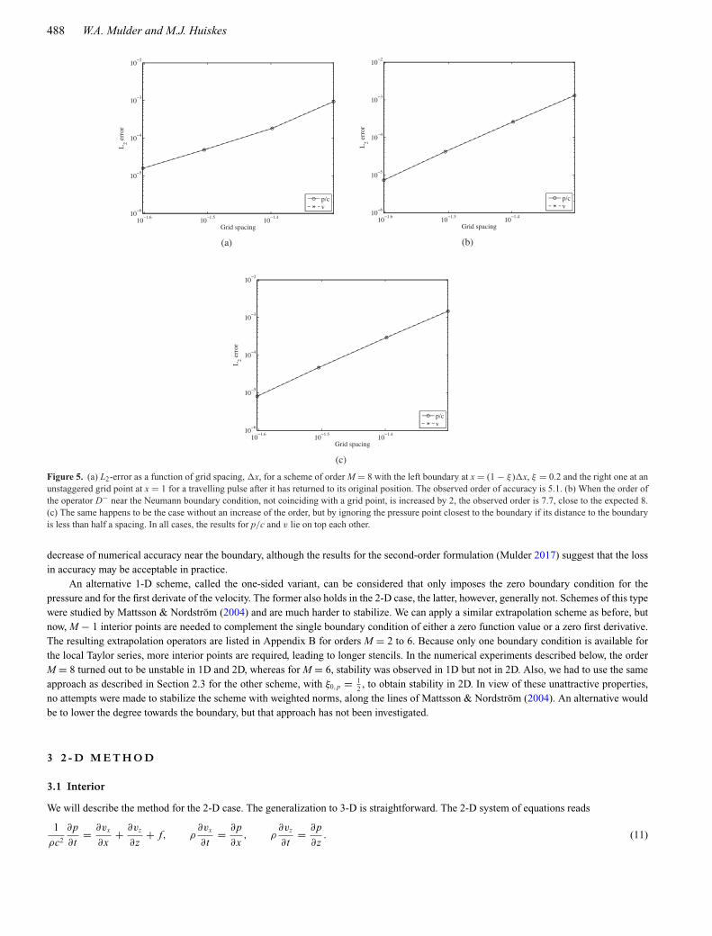
small time-step will keep the temporal error small.Fig. 5(a) shows the RMS errors as a function of grid spacing, �x, for an eighth-order scheme (M = 8). The domain ranged from

(1 − ξ )�x with ξ = 0.2 to 1. The time step was set at 1 per cent of its maximum value. The observed order of accuracy is 5.2 rather than theexpected 8. An increase of the order with 2 on the left boundary for the velocity extrapolation and the differentiation operator, D−, producesthe graphs in Fig. 5(b) with an estimated order of accuracy around 7.6.

Surprisingly, we observe a similar improvement in Fig. 5(c) without increasing the order but, instead, by dropping the point for thepressure if it is closer to the Dirichlet boundary than half a grid spacing. Dropping such points is not necessary for stability in 1D, but it is in2D and 3D, as discussed in Section 2.3. These numerical experiments therefore suggest that we do not have to increase the order for D− nearthe boundary and that for D+, we should ignore the point closer than half a grid spacing to the boundary.

2.5 One-sided variant

The previous scheme imposes (anti)symmetry across the boundaries. This amounts to the requirement that all even derivatives of the pressureare zero on the boundary, including the zeroth derivative. Similarly, all odd derivatives of the velocity should be zero. This follows from thefact that, for instance,

1

c2

∂2 p

∂t2= ∂2 p

∂x2(10)

should hold on the boundary. If p = 0 on the boundary, then ∂2 p∂t2 = 0 as well as all higher even time derivatives, implying that all even spatial

derivatives should vanish on the boundary. If p = 0 on the boundary for all time and the source sits at some distance from the boundary, theneq. (1) implies that ∂v

∂x = 0 on the boundary. Taking an odd number of spatial derivatives of ∂v

∂t = ∂p∂x on the boundary implies that all odd

spatial derivatives of v should vanish on the boundary since all even derivatives of p are zero.In the 2-D case, we would like to use the same numerical 1-D boundary conditions. However, if the boundary-normal does not coincide

with a coordinate direction, the above conditions on the derivatives along coordinate directions do not hold any more. The net effect will be a


Figure 5. (a) L2-error as a function of grid spacing, �x, for a scheme of order M = 8 with the left boundary at x = (1 − ξ )�x, ξ = 0.2 and the right one at anunstaggered grid point at x = 1 for a travelling pulse after it has returned to its original position. The observed order of accuracy is 5.1. (b) When the order ofthe operator D− near the Neumann boundary condition, not coinciding with a grid point, is increased by 2, the observed order is 7.7, close to the expected 8.(c) The same happens to be the case without an increase of the order, but by ignoring the pressure point closest to the boundary if its distance to the boundaryis less than half a spacing. In all cases, the results for p/c and v lie on top each other.

decrease of numerical accuracy near the boundary, although the results for the second-order formulation (Mulder 2017) suggest that the lossin accuracy may be acceptable in practice.

An alternative 1-D scheme, called the one-sided variant, can be considered that only imposes the zero boundary condition for thepressure and for the first derivate of the velocity. The former also holds in the 2-D case, the latter, however, generally not. Schemes of this typewere studied by Mattsson & Nordstrom (2004) and are much harder to stabilize. We can apply a similar extrapolation scheme as before, butnow, M − 1 interior points are needed to complement the single boundary condition of either a zero function value or a zero first derivative.The resulting extrapolation operators are listed in Appendix B for orders M = 2 to 6. Because only one boundary condition is available forthe local Taylor series, more interior points are required, leading to longer stencils. In the numerical experiments described below, the orderM = 8 turned out to be unstable in 1D and 2D, whereas for M = 6, stability was observed in 1D but not in 2D. Also, we had to use the sameapproach as described in Section 2.3 for the other scheme, with ξ0,p = 1

2 , to obtain stability in 2D. In view of these unattractive properties,no attempts were made to stabilize the scheme with weighted norms, along the lines of Mattsson & Nordstrom (2004). An alternative wouldbe to lower the degree towards the boundary, but that approach has not been investigated.

3 2 - D M E T H O D

3.1 Interior

We will describe the method for the 2-D case. The generalization to 3-D is straightforward. The 2-D system of equations reads

1

ρc2

∂p

∂t= ∂vx

∂x+ ∂vz

∂z+ f, ρ

∂vx

∂t= ∂p

∂x, ρ

∂vz

∂t= ∂p

∂z. (11)


Figure 6. Staggered grid near the boundary. The crosses mark the positions of the pressure variables, p, the right-pointing triangles of the horizontal particlevelocity, vx, and the downward-pointing triangles of vertical velocity, vz. The circles denote the boundary points involved in the vertical derivatives, the squaresthose required for the horizontal derivatives. Close to the surface, there may not be enough points for horizontal extrapolation with the desired polynomialdegree.

Figure 7. The maximum error in the pressure wavefield, divided by the amplitude of the latter, as a function of grid spacing, �x, for a range of dip anglesshows almost fourth-order convergence as indicated by the large triangle.

The solution values of the pressure, p, are placed on the unstaggered points of the modelling grid. The horizontal particle velocity, vx,is staggered by half a spacing in the x-direction and the vertical velocity, vz, by half a spacing in the z-direction. The grid is chosen such thatthe straight-line boundaries at xmin , xmax and zmax coincide with the unstaggered grid points. The same standard difference operators as in the1-D case are applied in each coordinate direction.

Figure 8. Sound speed (a) for the second test problem. The exact solution (b), shown at initial time, is periodic in the horizontal direction, has a zero normalderivative for the pressure at the bottom and a zero value of the pressure on the curved surface.


Figure 9. The maximum error in the pressure for the second test problem with a time step at half its maximum value for a discretization of order M = 4(circles) and order M = 8 (squares) as a function of the horizontal grid spacing �x. The dotted lines indicate the trends for first- and fourth-order convergence.

Figure 10. The maximum error in the pressure for the second test problem with a time step at 10 per cent of its maximum value for a discretization of orderM = 4 (circles) and order M = 8 (squares) as a function of the horizontal grid spacing �x. The dotted lines indicate the trends for first- and fourth-orderconvergence. Since the differences with Fig. 9 are small, the error must be dominated by the spatial discretization and boundary conditions.

3.2 Topography

In more than one space dimension, we can simply apply the 1-D scheme along grid lines, just as in (Mulder 2017) for the second-orderformulation of the wave equation. As already remarked in the introduction, this will increase the error if the normal to the free surface doesnot coincide with a grid line.

Near the free-surface boundary, the interior difference scheme of eq. (4) can be replaced by a scheme that consists in its application tothe interior points combined with the extrapolated values as defined in Appendix A for several orders. This is still a 1-D operation. Since itassumes more symmetry than is present when the boundary is not perfectly horizontal or vertical, an additional numerical error is incurred.It remains to be seen how that error affects the overall accuracy.

The extrapolated values are only used for the construction of the finite-difference operator in one direction and then discarded. They arenot involved in the extrapolation in the other coordinate direction. Note that a different way of implementation is to directly store the actionof the finite-difference operator on the extrapolated values, i.e. the modified difference operators, either obtained by the above constructionor by evaluating explicit expressions for the combined effect of extrapolation and differentiation.

In the 2-D experiments, we have imposed periodic or zero Dirichlet or Neumann boundary conditions at the left and right and at the‘bottom’, corresponding to the largest depth or z-value. These boundaries are assumed to be straight lines coinciding with the unstaggeredgrid points. For the smallest z-value, we assume topography, defined as a depth function of lateral position. The input is either a functionz(x) or a set of points zj = z(xj), j = 1, . . . , Ntopo. This set of points may have a smaller or larger spacing than the finite-difference grid. Wetherefore resample the topography by fitting a smooth cubic B-spline through the given z(xj). In the examples later on, we have somewhatarbitrarily resampled to a spline grid twice as coarse as the modelling grid.

For the test problems with an exact solution, the topography is known as a function (x(s), z(s)), where s parametrizes the boundary.Arc-length along the curve was chosen for the latter. Then, (xj, zj) on a grid 10 times finer than the modelling grid was evaluated from theanalytical expression for the shape of the boundary. Next, piecewise cubic Hermite interpolation was applied to find a representation of (x(s),z(s)). The reason for choosing (x(s), z(s)) instead of z(x) as a parametrization is the third test problem, which has a vertical boundary in onecorner.


Figure 11. As Figs 9 and 10, but for the one-sided variant and order M = 4 at 10 per cent of the maximum time step.

Figure 12. Sound speed (a) for the third test problem. The exact solution (b), here shown at zero time, represents a standing wave and has zero pressure oneach boundary.

The extrapolation requires M/2 points from the interior that may not always be available for the horizontal derivatives, as sketched inFig. 6. If, for instance, a sixth-order scheme is to be used in the horizontal direction, 3 interior points are needed for extrapolation, whereasonly two are available for vx close to the summit. In that case, extrapolation is applied across each boundary in the following way. For theextrapolation, M conditions are required:

(i) use M/2 boundary conditions (all even or odd derivatives zeros) at the nearest boundary;(ii) interpolate through the available interior points;

Figure 13. Maximum error in the pressure for the third test problem with a time step at half the maximum value for a discretization of order M = 4 or 8as a function of the horizontal grid spacing �x (a). The dotted lines indicate first- and fourth-order convergence and the actual convergence is about secondorder for both. With pressure and velocities set to zero in the exterior and no special treatment of the free surface, worse than first-order error behaviour isobserved (b).


Figure 14. Sound speed model (a) and density (b) for a model with a very rough topography as well as a snapshot (c) of the pressure wavefield after 1 s for asource at the centre, at a depth of 22 m below the surface. All boundaries are reflecting.

(iii) for the remaining unknowns, use the boundary conditions at the opposite boundary point, starting from the conditions on the lowestderivative.

In this way, an extrapolation operator to the left and one the right can be constructed. The finite-difference weights are then applied tothis operator to obtain the modified finite-difference scheme. Finding the intersection point of the vertical lines, on which the pressure orvertical displacement is defined, with the boundary is trivial for a spline of the form z(x). For the horizontal lines, Newton’s method can beused or, alternatively, an explicit evaluation of the cubic roots. In the case of a parametrization of the form (x(s), z(s)), one of those methodshas to be used for both the horizontal and the vertical lines.

3.3 Reconstruction

In more than one space dimension, ignoring points closer to the zero Dirichlet boundary than half a spacing may cause problems in theother coordinate direction(s). An obvious solution is the reconstruction of the pressure at the ignored points with the same 1-D interpolatingpolynomial as used for the extrapolation beyond the Dirichlet boundary. Such a reconstruction can be performed after each temporal updateof the pressure. In this way, the pressure is available during the next time step if it happens to be needed for another coordinate direction. Analternative is to let the time step update the pressure values, based on velocity derivatives and earlier pressure values, but this was observedto produce weak instabilities.

If a pressure point is closer than half a spacing to the boundary along coordinate lines in more than one direction, we can either perform1-D interpolation based on the nearest boundary point or carry out multidimensional interpolation.

4 2 - D R E S U LT S

We consider the same numerical test problems used before in the second-order formulation (Mulder 2017). The first three have an exactsolution. They are followed by a problem with a very rough topography created with a random number generator and designed to push themethod to its limits. The last two problems have a realistic topography but fantasy geology.


Figure 15. 2-D problem based on a cross-section through the topography of the Vaalserberg. The sound speed (a) and density model(b) are based on ageo-fantasy. The seismic traces (c) are dominated by the direct arrival and the stronger reflections.

The first problem is a homogeneous half-space with a velocity of 2 km s−1 and a density of 1 kg dm−3. The surface has a dip angleranging from 0◦ to 45◦ at a 5◦ increment for the various tests. The source at 60 m distance to the surface has a wavelet w(t) = t[1 − (2t/Tw)2]7

for |t| < Tw/2 and zero otherwise, with a duration of Tw = 0.125 s. It is the time integral of the one used in the second-order formulation(Mulder 2017). The simulations were started at −Tw/2 with a time step at 10 per cent of the maximum value allowed for stability to keep thetemporal error of the second-order time-stepping order sufficiently small. The error was measured at a time t = 0.4 s. The solution consistsof a direct wave that constitutes about half a circle together with its ghost. Fig. 7 plots the maximum error in the pressure wavefield, dividedby the wavefield’s amplitude, as a function of the grid spacing �x for several dip angles. The observed convergence rate is close to fourthorder at zero dip. At larger dips, where the approximation of symmetry or antisymmetry in the coordinate direction rather than in the normaldirection of the free surface starts to play a role, the order of convergence becomes worse, closer to 3.5 on finer grids.

Fig. 8 shows the sound speed model for the second test problem, together with the pressure at initial time. The exact solution is atravelling wave, with a zero Dirichlet boundary condition at the surface (smallest z-values) and a zero Neumann boundary condition at thebottom. The left and right boundary conditions are periodic. The maximum error in the pressure after travelling around once on the periodicgrid is shown in Fig. 9 for a sequence of grid spacings, �x and a scheme of order 4 and 8, respectively. The time step was set at half itsmaximum value. For reference, the dotted lines show the convergence behaviour for orders 1 and 4.

In the case of an interior fourth-order spatial discretization (M = 4), a fourth-order error in the pressure is observed on the coarser grids.On finer grids, the effects of the locally 1-D approximations in the boundary conditions start to appear and the convergence rate drops toabout second-order. The same is true in the eighth-order case. Note that the error on the coarsest grid starts with a smaller value compared tothe fourth-order case, making a scheme of order 8 still attractive for production runs.

To verify that the second-order time-stepping error does not dominate the results, we repeated the runs at 10 per cent of the maximumtime step. Fig. 10 displays the resulting errors. As the difference with the earlier runs at half the maximum time step is small, we concludethat the error on finer grids must be dominated by the boundaries.

Fig. 11 displays the convergence behaviour for the one-sided variant with a fourth-order spatial discretization. The scheme appears tobe slightly more accurate, compared to the result for order M = 4 in Fig. 10. Unfortunately, it turned out to be unstable for orders M = 6 andM = 8, and is therefore less attractive.


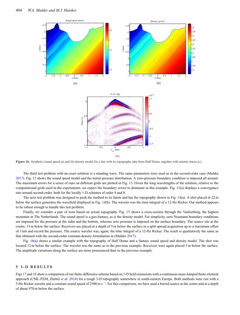
Figure 16. Synthetic sound speed (a) and (b) density model for a line with its topography take from Half Dome, together with seismic traces (c).

The third test problem with an exact solution is a standing wave. The same parameters were used as in the second-order case (Mulder2017). Fig. 12 shows the sound speed model and the initial pressure distribution. A zero-pressure boundary condition is imposed all around.The maximum errors for a series of runs on different grids are plotted in Fig. 13. Given the long wavelengths of the solution, relative to thecomputational grids used in the experiments, we expect the boundary errors to dominate in this example. Fig. 13(a) displays a convergencerate around second-order, both for the locally 1-D schemes of order 4 and 8.

The next test problem was designed to push the method to its limits and has the topography shown in Fig. 14(a). A shot placed at 22 mbelow the surface generates the wavefield displayed in Fig. 14(b). The wavelet was the time integral of a 12-Hz Ricker. Our method appearsto be robust enough to handle this test problem.

Finally, we consider a pair of tests based on actual topography. Fig. 15 shows a cross-section through the Vaalserberg, the highestmountain in The Netherlands. The sound speed is a geo-fantasy, as is the density model. For simplicity, zero Neumann boundary conditionsare imposed for the pressure at the sides and the bottom, whereas zero pressure is imposed on the surface boundary. The source sits at thecentre, 13 m below the surface. Receivers are placed at a depth of 5 m below the surface in a split-spread acquisition up to a maximum offsetof 1 km and record the pressure. The source wavelet was, again, the time integral of a 12-Hz Ricker. The result is qualitatively the same asthat obtained with the second-order constant-density formulation in (Mulder 2017).

Fig. 16(a) shows a similar example with the topography of Half Dome and a fantasy sound speed and density model. The shot waslocated 12 m below the surface. The wavelet was the same as in the previous example. Receivers were again placed 5 m below the surface.The amplitude variations along the surface are more pronounced than in the previous example.

5 3 - D R E S U LT S

Figs 17 and 18 show a comparison of our finite-difference scheme based on 1-D field extensions with a continuous mass-lumped finite-elementapproach (CML-FEM, Zhebel et al. 2014) for a rough 3-D topography somewhere in south-eastern Europe. Both methods were run with a5-Hz Ricker wavelet and a constant sound speed of 2500 m s−1. For this comparison, we have used a buried source at the centre and at a depthof about 970 m below the surface.


Figure 17. (a) Elevation map of a 9 × 9 km area in south-eastern Europe. Elevations range from 1750 to 2200 m. (b) Pressure snapshot after 1 s of propagationwith the finite-difference method. (c) Pressure snapshot after 1 s of propagation with the finite-element method.

The 3-D finite-difference simulation was performed using an implementation of the approach in an FWI production system, takingnumerical parameters for regular production settings. The results were obtained with an eighth-order spatial discretization at five grid pointsper wavelength. Both the snapshots in Figs 17(b) and (c) as well as the normalized shot panels in Figs 18(a) and (b) show a close agreementbetween the finite-difference and finite-element results. Their differences, shown in Fig. 18(c), have a maximum error of 0.04. Results at4 points per wavelength are very similar with slightly larger a maximum error of 0.05.

6 C O N C LU S I O N S

Stability and accuracy of a modified finite-difference scheme that can handle topography in the first-order formulation of the acoustic waveequation has been studied by a series of 1-D, 2-D and 3-D tests. The boundary conditions consist in imposing antisymmetry for the pressureand symmetry for each particle velocity component on the boundary in its corresponding coordinate direction. Because the coordinatedirection and corresponding velocity components rather than the normal direction and normal velocity component are chosen, an additionalnumerical error is incurred, on top of the errors caused by the interior spatial discretization and the time stepping scheme.

The modification of the finite-difference scheme near the boundary results in an instability in more than one space dimension, whichcan be removed by ignoring pressure values closer to the boundary than half a grid spacing. Because these values may still be needed forderivatives in another coordinate direction, reconstruction by polynomial interpolation is applied.

In a simple 2-D test with a dipped flat surface, the observed convergence rate for the spatial error is around order four, although themaximum error loses about half an order for larger dips. In a 2-D test with a variable velocity, a curved interface, and a solution that hasa long wavelength compared to the grid spacing of the computational grid, the boundary error dominates and reduces the overall spatialaccuracy to order two. To put this into perspective, we note that a high-order finite-difference scheme also reduces to second-order accuracyin the interior when differencing across discontinuities in the velocity or density, because the pressure is continuous but not differentiable overthere.

3-D examples exhibit acceptable accuracy for our boundary scheme when using typical production-run parameters.


Figure 18. (a) Normalized shot panel for a receiver line 500 m below the source along the central vertical line in the elevation map of Fig. 17, obtained withthe finite difference method. (b) Same shot panel obtained with the finite-element method. (c) Difference of the shot panels in (a) and (b).

R E F E R E N C E S

AlMuhaidib, A.M., Fehler, M., Toksoz, M.N. & Zhang, Y., 2011. Finitedifference elastic wave modeling including surface topography, in SEGTechnical Program Expanded Abstracts 2011, pp. 2941–2946.

Bartel, L.C., Symons, N.P. & Aldridge, D.F., 2000. Graded boundary sim-ulation of air/Earth interfaces in finite-difference elastic wave modeling,in SEG Technical Program Expanded Abstracts 2000, pp. 2444–2447.

Becache, E., Joly, P. & Tsogka, C., 2000. An analysis of new mixed finiteelements for the approximation of wave propagation problems, SIAM J.Numer. Anal., 37(4), 1053–1084.

Benjemaa, M., Glinsky-Olivier, N., Cruz-Atienza, V.M., Virieux, J. &Piperno, S., 2007. Dynamic non-planar crack rupture by a finite volumemethod, Geophys. J. Int., 171(1), 271–285.

Bohlen, T. & Saenger, E.H., 2006. Accuracy of heterogeneous staggered-grid finite-difference modeling of Rayleigh waves, Geophysics, 71(4),109–115.

Boore, D.M., 1972. Finite difference methods for seismic wave propaga-tion in heterogeneous materials, in Seismology: Surface Waves and EarthOscillations, vol. 11 of Methods in Computational Physics: Advances inResearch and Applications, pp. 1–37, ed. Bold, B.A., Elsevier.

Carpenter, M.H., Nordstrom, J. & Gottlieb, D., 1999. A stable and conser-vative interface treatment of arbitrary spatial accuracy, J. Comput. Phys.,148(2), 341–365.

Charney, J.G., Fjortoft, R. & von Neumann, J., 1950. Numerical integrationof the barotropic vorticity equation, Tellus, 2, 237–254.

Chin-Joe-Kong, M.J.S., Mulder, W.A. & van Veldhuizen, M., 1999. Higher-order triangular and tetrahedral finite elements with mass lumping forsolving the wave equation, J. Eng. Math., 35, 405–426.

Cohen, G., Joly, P., Roberts, J.E. & Tordjman, N., 2001. Higher order trian-gular finite elements with mass lumping for the wave equation, SIAM J.Numer. Anal., 38(6), 2047–2078.

De Basabe, J.D. & Sen, M.K., 2007. Grid dispersion and stability criteriaof some common finite-element methods for acoustic and elastic waveequations, Geophysics, 62(6), T81–T95.

De la Puente, J., Ferrer, M., Hanzich, M., Castillo, J.E. & Cela, J.M., 2014.Mimetic seismic wave modeling including topography on deformed stag-gered grids, Geophysics, 79, T125–T141.

Dormy, E. & Tarantola, A., 1995. Numerical simulation of elastic wavepropagation using a finite volume method, J. geophys. Res., 100(B2),2123–2133.

Dumbser, M., Kaser, M. & de la Puente, J., 2007. Arbitrary high-order finitevolume schemes for seismic wave propagation on unstructured meshes in2D and 3D, Geophys. J. Int., 171(2), 665–694.

Etienne, V., Chaljub, E., Virieux, J. & Glinsky, N., 2010. An hp-adaptivediscontinuous Galerkin finite-element method for 3-D elastic wave mod-elling, Geophys. J. Int., 183(2), 941–962.

Fornberg, B., 2010. A finite difference method for free boundary problems,J. Comput. Appl. Math., 233(11), 2831–2840.

Gao, L., Brossier, R., Pajot, B., Tago, J. & Virieux, J., 2015. An immersedfree-surface boundary treatment for seismic wave simulation, Geophysics,80(5), T193–T209.

Grote, M.J., Schneebeli, A. & Schotzau, D., 2006. Discontinuous Galerkinfinite element method for the wave equation, SIAM J. Numer. Anal., 44(6),2408–2431.

Haney, M.M., 2007. Generalization of von Neumann analysis for a modelof two discrete half-spaces: the acoustic case, Geophysics, 72(5), SM35–SM46.


Hestholm, S. & Ruud, B., 1998. 3-D finite-difference elastic wave modelingincluding surface topography, Geophysics, 63, 613–622.

Hestholm, S. & Ruud, B., 2002. 3D free-boundary conditions for coordinate-transform finite-difference seismic modelling, Geophys. Prospect., 50(5),463–474.

Hu, W., 2015. IBFD for seismic wave modeling—regular grid method han-dling arbitrary topography, in SEG Technical Program Expanded Ab-stracts 2015, pp. 3544–3548.

Joly, P., 2003. Variational methods for time-dependent wave propagationproblems, in Topics in Computational Wave Propagation, vol. 31 of Lec-ture Notes in Computational Science and Engineering, pp. 201–264,eds Ainsworth, M., Davies, P., Duncan, D., Rynne, B. & Martin, P.,Springer.

Komatitsch, D. & Vilotte, J., 1998. The spectral element method: an effi-cient tool to simulate the seismic response of 2-D and 3-D geologicalstructures, Bull. seism. Soc. Am., 88, 368–392.

Lipnikov, K., Manzini, G. & Shashkov, M., 2014. Mimetic finite differencemethod, J. Comput. Phys., 257, 1163–1227.

Lombard, B., Piraux, J., Gelis, C. & Virieux, J., 2008. Free and smoothboundaries in 2-D finite-difference schemes for transient elastic waves,Geophys. J. Int., 172(1), 252–261.

Mattsson, K. & Nordstrom, J., 2004. Summation by parts operators for fi-nite difference approximations of second derivatives, J. Comput. Phys.,199(2), 503–540.

Mattsson, K. & Nordstrom, J., 2006. High order finite difference methodsfor wave propagation in discontinuous media, J. Comput. Phys., 220(1),249–269.

Mattsson, K., Almquist, M. & Carpenter, M.H., 2014. Optimal diagonal-norm SBP operators, J. Comput. Phys., 264, 91–111.

Minisini, S., Zhebel, E., Kononov, A. & Mulder, W.A., 2013. Local timestepping with the discontinuous Galerkin method for wave propagationin 3D heterogeneous media, Geophysics, 78(3), T67–T77.

Mittet, R., 2002. Free-surface boundary conditions for elastic staggered-gridmodeling schemes, Geophysics, 67(5), 1616–1623.

Moczo, P., Robertsson, J.O. & Eisner, L., 2007. The finite-difference time-domain method for modeling of seismic wave propagation, in Advancesin Wave Propagation in Heterogenous Earth, vol. 48 of Advances inGeophysics, pp. 421–516, eds Wu, R.-S., Maupin, V. & Dmowska, R.,Elsevier.

Moczo, P., Kristek, J., Galis, M., Chaljub, E. & Etienne, V., 2011. 3-D finite-difference, finite-element, discontinuous-Galerkin and spectral-elementschemes analysed for their accuracy with respect to P-wave to S-wavespeed ratio, Geophys. J. Int., 187(3), 1645–1667.

Modave, A., St-Cyr, A., Mulder, W.A. & Warburton, T., 2015. A nodal dis-continuous Galerkin method for reverse-time migration on GPU clusters,Geophys. J. Int., 203(2), 1419–1435.

Mulder, W.A., 1996. A comparison between higher-order finite elementsand finite differences for solving the wave equation, in Proceedings of theSecond ECCOMAS Conference on Numerical Methods in Engineering,Paris, Sept. 9–13, 1996, pp. 344–350, John Wiley & Sons, Chichester.

Mulder, W.A., 2017. A simple finite-difference scheme for handling topogra-phy with the second-order wave equation, Geophysics, 82(3), T111–T120.

Mulder, W.A. & Shamasundar, R., 2016. Performance of continuous mass-lumped tetrahedral elements for elastic wave propagation with and withoutglobal assembly, Geophys. J. Int., 207(1), 414–421.

Nesemann, L., 2014. Numerical acoustic-elastic coupling and curved bound-

aries for RTM, in 76th EAGE Conference & Exhibition, Amsterdam,Netherlands, Extended Abstracts, We G105 03.

Pelties, C., Hermann, M.K.V. & Castro, C.E., 2010. Regular versus irregularmeshing for complicated models and their effect on synthetic seismo-grams, Geophys. J. Int., 183(2), 1031–1051.

Petersson, N.A. & Sjogreen, B., 2015. Wave propagation in anisotropicelastic materials and curvilinear coordinates using a summation-by-partsfinite difference method, J. Comput. Phys., 299, 820–841.

Piraux, J. & Lombard, B., 2001. A new interface method for hyperbolic prob-lems with discontinuous coefficients: one-dimensional acoustic example,J. Comput. Phys., 168(1), 227–248.

Riviere, B. & Wheeler, M., 2003. Discontinuous finite element methods foracoustic and elastic wave problems, Contemp. Math., 329, 271–282.

Robertsson, J.O., 1996. A numerical free-surface condition for elastic/viscoelastic finite-difference modeling in the presence of topography,Geophysics, 61(6), 1921–1934.

Schultz, C.A., 1997. A density-tapering approach for modeling the seismicresponse of free-surface topography, Geophys. Res. Lett., 24(22), 2809–2812.

Seo, J.H. & Mittal, R., 2011. A high-order immersed boundary method foracoustic wave scattering and low-mach number flow-induced sound incomplex geometries, J. Comput. Phys., 230, 1000–1019.

Seriani, G., Priolo, E., Carcione, J. & Padovani, E., 1992. High-order spec-tral element method for elastic wave modeling, SEG Technical ProgramExpanded Abstracts, 11, 1285–1288.

Shortley, G.H. & Weller, R., 1938. Numerical solution of Laplace’s equa-tion, J. Appl. Phys., 9(5), 334–344.

Solano, C.A.P., Donno, D. & Chauris, H., 2016. Finite-difference strategyfor elastic wave modelling on curved staggered grids, Comput. Geosci.,20(1), 245–264.

Strand, B., 1994. Summation by parts for finite difference approximationsfor d/dx, J. Comput. Phys., 110(1), 47–67.

Tessmer, E. & Kosloff, D., 1994. 3-D elastic modeling with surface topog-raphy by a Chebychev spectral method, Geophysics, 59(3), 464–473.

Zeng, C., Xia, J., Miller, R.D. & Tsoflias, G.P., 2012. An improved vac-uum formulation for 2D finite-difference modeling of Rayleigh wavesincluding surface topography and internal discontinuities, Geophysics,77, T1–T9.

Zhang, J. & Gao, H., 2009. Elastic wave modelling in 3-D frac-tured media: an explicit approach, Geophys. J. Int., 177(3), 1233–1241.

Zhang, J. & Liu, T., 1999. P-SV-wave propagation in heterogeneous media:grid method, Geophys. J. Int., 136(2), 431–438.

Zhang, W. & Chen, X., 2006. Traction image method for irregular free sur-face boundaries in finite difference seismic wave simulation, Geophys. J.Int., 167(1), 337–353.

Zhang, D., Schuster, G. & Zhan, G., 2013. Multi-source least-squares reversetime migration with topography, in SEG Technical Program ExpandedAbstracts, pp. 3736–3740.

Zhebel, E., Minisini, S., Kononov, A. & Mulder, W.A., 2011. Solving the3D acoustic wave equation with higher-order mass-lumped tetrahedralfinite elements, in 73rd EAGE Conference & Exhibition incorporatingSPE EUROPEC, Vienna, Austria, Extended Abstracts, A010.

Zhebel, E., Minisini, S., Kononov, A. & Mulder, W.A., 2014. A comparisonof continuous mass-lumped finite elements with finite differences for 3-Dwave propagation, Geophys. Prospect., 62(5), 1111–1125.

A P P E N D I X A : B O U N DA RY E X T R A P O L AT I O N O P E R AT O R S

For the lowest order, M = 2, extrapolation of p, where j is distance of the target point to the last interior point and ξ is the distance of theboundary to the last interior point, obeys Ed(ξ , j) = ( (ξ − j)/ξ ). For v, we have En(ξ , j) = ( 1 ).


If ξ < 12 , shown in Fig. 1(a), no extrapolation is needed for D+. Otherwise, its last rows and columns become

D+ = 1

�x

⎛⎜⎜⎜⎜⎜⎜⎝

. . ....

......

...

. . . −1 1 0 0

. . . 0 −1 1 0

. . . 0 0 − 1ξ

0

⎞⎟⎟⎟⎟⎟⎟⎠

. (A1)

Because ξ ≥ 12 , the entry with −1/ξ will not cause problems. In the second-order formulation, the fact that ξ could approach zero forced the

time step bound to zero and for that reason, points close to the boundary had to be ignored. Here, this does not seem to be necessary in the1-D case, but it is in a 2-D or 3-D setting, as argued in Section 2.3. The operator D−, acting on the points shown as dots in Fig. 1, does notrequire extrapolation for ξ ≥ 1

2 whereas for ξ < 12 and M = 2, it produces zero in the last interior point, marked by a cross in Fig. 1(a).

For M = 4, extrapolation for p is given by

Ed (ξ, j) = ξ − j

1 + 2ξ

(j( j − 2ξ )

1 + ξ,

(1 + j)(1 + 2ξ − j)

ξ

), (A2a)

with special cases

Ed ( j, j) = (0, 0) , Ed (ξ, 1) = ξ − 1

1 + 2ξ

(1 − 2ξ

1 + ξ, 4

). (A2b)

For a pressure grid with index Nx − 1 for the last interior points, this leads to⎛⎝ pNx

pNx + 1

⎞⎠ = E

⎛⎝ pNx − 2

pNx − 1

⎞⎠ , E j,k = Ed

k (ξ, j). (A3)

Extrapolation for v is given by

En(ξ, j) =(

j( j − 2ξ )

1 + 2ξ,

(1 + j)(1 + 2ξ − j)

1 + 2ξ

). (A4)

For M = 6 and p,

Ed (ξ, j) = j − ξ

1 + ξ

(− j( j + 1)( j − 2ξ − 1)( j − 2ξ )

4(ξ + 2)(2ξ + 3),

j( j + 2)( j − 2ξ )( j − 2ξ − 2)

(2ξ + 1)(2ξ + 3), − ( j + 1)( j + 2)( j − 2ξ − 1)( j − 2ξ − 2))

4ξ (2ξ + 1)

),

(A5)

with special cases ξ = 12 , j = 1, or j = 2. For v,

En(ξ, j) =(

j( j + 1)( j − 2ξ − 1)( j − 2ξ )

4(ξ + 1)(2ξ + 3), − j( j + 2)( j − 2ξ − 2)( j − 2ξ )

(2ξ + 1)(2ξ + 3),

( j + 1)( j + 2)( j − 2ξ − 2)( j − 2ξ − 1)

4(ξ + 1)(2ξ + 1)

). (A6)

Finally, for M = 8 and p,

Ed (ξ, j) = j − ξ

3 + 2ξ

(− j( j + 1)( j + 2)( j − 2ξ − 2)( j − 2ξ − 1)( j − 2ξ )

12(ξ + 2)(ξ + 3)(2ξ + 5),

j( j + 1)( j + 3)( j − 2ξ − 3)( j − 2ξ − 1)( j − 2ξ )

4(ξ + 1)(ξ + 2)(2ξ + 5),

− j( j + 2)( j + 3)( j − 2ξ − 3)( j − 2ξ − 2)( j − 2ξ )

4(ξ + 1)(ξ + 2)(2ξ + 1),

( j + 1)( j + 2)( j + 3)( j − 2ξ − 3)( j − 2ξ − 2)( j − 2ξ − 1)

12ξ (ξ + 1)(2ξ + 1)

), (A7)

whereas for v,

En(ξ, j) =(

j( j + 1)( j + 2)( j − 2ξ − 2)( j − 2ξ − 1)( j − 2ξ )

12(ξ + 2)(2ξ + 3)(2ξ + 5), − j( j + 1)( j + 3)( j − 2ξ − 3)( j − 2ξ − 1)( j − 2ξ )

4(ξ + 1)(2ξ + 3)(2ξ + 5),

j( j + 2)( j + 3)( j − 2ξ − 3)( j − 2ξ − 2)( j − 2ξ )

4(ξ + 2)(2ξ + 1)(2ξ + 3), − ( j + 1)( j + 2)( j + 3)( j − 2ξ − 3)( j − 2ξ − 2)( j − 2ξ − 1)

12(ξ + 1)(2ξ + 1)(2ξ + 3)

). (A8)

In all cases, the components obey

(ξ − j)Enk (ξ, j) = (

ξ − k + 12 M

)Ed

k (ξ, j), k = 1, . . . , 12 M. (A9)

Note that the last element of Ed(ξ , j) always contains a factor 1/ξ , which does not cause divergence as we always have ξ ≥ 12 on a staggered

grid.


A P P E N D I X B : B O U N DA RY E X T R A P O L AT I O N O P E R AT O R S F O R VA R I A N T 2

For M = 2, we have the same operators as in the previous case. For M = 4 and extrapolation of p,

Ed (ξ, j) = ξ − j

2

(j( j + 1)

ξ + 2, −2 j( j + 2)

ξ + 1,

( j + 1)( j + 2)

ξ

), (B1)

whereas for v,

En(ξ, j) = 1

2(2 + 3ξ (2 + ξ ))(− j( j + 1) [ j(1 + 2ξ ) − ξ (2 + 3ξ )] , 2( j + 2) [ j(2 + 2ξ ) − ξ (4 + 3ξ )] ,

−( j + 1)( j + 2) [ j(3 + 2ξ ) − 2 − 3ξ (2 + ξ )]). (B2)

For M = 6,

Ed (ξ, j) = ξ − j

24

(j( j + 1)( j + 2)( j + 3)

ξ + 4, −4 j( j + 1)( j + 2)( j + 4)

ξ + 3,

6 j( j + 1)( j + 3)( j + 4)

ξ + 2,

−4 j( j + 2)( j + 3)( j + 4)

ξ + 1,

( j + 1)( j + 2)( j + 3)( j + 4)

ξ

), (B3)

and

En(ξ, j) = 1

24(24 + 5ξ (4 + ξ )(5 + ξ (4 + ξ )))

(− j( j + 1)( j + 2)( j + 3)(2 j(2ξ + 3)(ξ (ξ + 3) + 1) − ξ (ξ (ξ (5ξ + 24) + 33) + 12)),

4 j( j + 1)( j + 2)( j + 4)( j(ξ (ξ (4ξ + 21) + 28) + 8) − ξ (5ξ + 8)(ξ (ξ + 4) + 2)),

−6 j( j + 1)( j + 3)( j + 4)(2 j(ξ + 2)(2ξ (ξ + 4) + 3) − ξ (ξ (ξ (5ξ + 32) + 57) + 24)),

4 j( j + 2)( j + 3)( j + 4)( j(ξ (ξ (4ξ + 27) + 52) + 24) − ξ (ξ (ξ (5ξ + 36) + 78) + 48)),

−( j + 1)( j + 2)( j + 3)( j + 4)(2 j(2ξ + 5)(ξ (ξ + 5) + 5) − 5ξ (ξ + 4)(ξ (ξ + 4) + 5) − 24)). (B4)

The scheme for order M = 8 is unstable in 1D.

Delft University of Technology A simple finite-difference ...

Documents

Transcript of Delft University of Technology A simple finite-difference ...