Delay Differential Equation Models in

Mathematical Biology

by

Jonathan Erwin Forde

A dissertation submitted in partial fulfillmentof the requirements for the degree of

Doctor of Philosophy(Mathematics)

in The University of Michigan2005

Doctoral Committee:

Assistant Professor Patrick W. Nelson, ChairProfessor Robert KrasnyProfessor Jeffrey B. RauchProfessor John W. Schiefelbein, Jr.Professor Carl P. Simon

c© Jonathan Erwin Forde 2006All Rights Reserved

For my father, who pointed the way, and my mother, who helped me along it.

ii

ACKNOWLEDGEMENTS

I would like to thank the many people who helped me reach this point. My

advisor, Dr. Patrick Nelson, for taking me on as a student, introducing me to

mathematical biology, and enduring my frequent tardiness. Dr. David Bortz, for

always being available to help. Dr. Yang Kuang of Arizona State University, for his

frequent insights into a difficult area and his faith in my abilities. The members of

my committee, Professors Robert Krasny, Jeffrey Rauch, John Schiefelbein and Carl

Simon, for their invaluable comments and patience. Thank you to Mom, Andrew,

Katie and Grandma, my family: no matter where I have gone, home has always been

with you. Without you all, this work would not have been possible. Finally, I cannot

give enough thanks to my friend, colleague and office-mate Dr. Stanca Ciupe, for her

friendship, supportiveness, all the conversation, and helping me find my way through

graduate school.

iii

TABLE OF CONTENTS

DEDICATION . . . . . . . . . . . . . . . . . . . . . . . . . . . . . . . . . . . . . . . . . . ii

ACKNOWLEDGEMENTS . . . . . . . . . . . . . . . . . . . . . . . . . . . . . . . . . . iii

LIST OF FIGURES . . . . . . . . . . . . . . . . . . . . . . . . . . . . . . . . . . . . . . vi

CHAPTER

1. Preliminaries . . . . . . . . . . . . . . . . . . . . . . . . . . . . . . . . . . . . . . . 1

1.1 Delay Differential Equations in Mathematical Biology . . . . . . . . . . . . . 11.2 Basic Properties of Delay Differential Equations . . . . . . . . . . . . . . . . 21.3 Linear Delay Differential Equations with Constant Delays and Coefficients . 41.4 The differential equation z(t) = az(t− τ)− bz(t) . . . . . . . . . . . . . . . . 51.5 A Comparison Lemma . . . . . . . . . . . . . . . . . . . . . . . . . . . . . . 71.6 Local Stability for Delay Differential Equations . . . . . . . . . . . . . . . . 8

1.6.1 The Pontriagin Criteria . . . . . . . . . . . . . . . . . . . . . . . . 81.6.2 Chebotarev’s Theorem . . . . . . . . . . . . . . . . . . . . . . . . . 91.6.3 Domain Subdivision . . . . . . . . . . . . . . . . . . . . . . . . . . 101.6.4 Frequency Methods . . . . . . . . . . . . . . . . . . . . . . . . . . . 111.6.5 The Tsypkin Criterion . . . . . . . . . . . . . . . . . . . . . . . . . 12

2. Linear Stability Analysis via Sturm Sequences . . . . . . . . . . . . . . . . . 14

2.1 General Method . . . . . . . . . . . . . . . . . . . . . . . . . . . . . . . . . . 142.1.1 Existence of Critical Delays . . . . . . . . . . . . . . . . . . . . . . 142.1.2 Nondegeneracy . . . . . . . . . . . . . . . . . . . . . . . . . . . . . 18

2.2 Positive Real Roots and Sturm Sequences . . . . . . . . . . . . . . . . . . . . 202.3 Applications . . . . . . . . . . . . . . . . . . . . . . . . . . . . . . . . . . . . 232.4 General Order Two and Three Characteristic Equations . . . . . . . . . . . . 262.5 Conclusions . . . . . . . . . . . . . . . . . . . . . . . . . . . . . . . . . . . . 30

3. Single Species Models . . . . . . . . . . . . . . . . . . . . . . . . . . . . . . . . . 32

3.1 A Fixed-Point Theorem from Nonlinear Functional Analysis . . . . . . . . . 333.2 A General Single-Species Population Model with Delay . . . . . . . . . . . . 343.3 A Specific Single-Species Delay Model . . . . . . . . . . . . . . . . . . . . . . 40

3.3.1 Oscillatory Solutions . . . . . . . . . . . . . . . . . . . . . . . . . . 413.3.2 An Extension of Previously Known Results . . . . . . . . . . . . . 45

3.4 Delay Dependent Parameters . . . . . . . . . . . . . . . . . . . . . . . . . . . 483.5 Another General Model . . . . . . . . . . . . . . . . . . . . . . . . . . . . . . 503.6 Constant per capita Death Rates . . . . . . . . . . . . . . . . . . . . . . . . . 533.7 Delay Dependent Parameters . . . . . . . . . . . . . . . . . . . . . . . . . . . 59

iv

4. Predator-Prey Interaction Models . . . . . . . . . . . . . . . . . . . . . . . . . 64

4.1 The Lotka-Volterra Predator-Prey Interaction Model . . . . . . . . . . . . . 644.2 A Delay Model of Predator-Prey Interaction . . . . . . . . . . . . . . . . . . 684.3 Preliminary Analysis . . . . . . . . . . . . . . . . . . . . . . . . . . . . . . . 69

4.3.1 Positivity of Solutions . . . . . . . . . . . . . . . . . . . . . . . . . 704.3.2 Uniform Boundedness of Solutions . . . . . . . . . . . . . . . . . . 704.3.3 Steady States . . . . . . . . . . . . . . . . . . . . . . . . . . . . . . 744.3.4 Linear Stability . . . . . . . . . . . . . . . . . . . . . . . . . . . . . 75

4.4 Existence of Periodic Solution . . . . . . . . . . . . . . . . . . . . . . . . . . 784.4.1 The “Phase Plane” . . . . . . . . . . . . . . . . . . . . . . . . . . . 804.4.2 Oscillation of Solutions . . . . . . . . . . . . . . . . . . . . . . . . . 81

4.5 Future Work . . . . . . . . . . . . . . . . . . . . . . . . . . . . . . . . . . . . 86

5. Conclusion . . . . . . . . . . . . . . . . . . . . . . . . . . . . . . . . . . . . . . . . 88

BIBLIOGRAPHY . . . . . . . . . . . . . . . . . . . . . . . . . . . . . . . . . . . . . . . . 91

v

LIST OF FIGURES

Figure

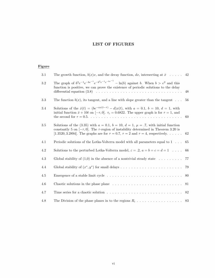
3.1 The growth function, b(x)x, and the decay function, dx, intersecting at x . . . . . 42

3.2 The graph of b3e−1e−be−1e−b2e−1e−be−1

− ln(b) against b. When b > e2 and thisfunction is positive, we can prove the existence of periodic solutions to the delaydifferential equation (3.8) . . . . . . . . . . . . . . . . . . . . . . . . . . . . . . . . 48

3.3 The function b(x), its tangent, and a line with slope greater than the tangent . . . 56

3.4 Solutions of the x(t) = (be−ax(t−τ) − d)x(t), with a = 0.1, b = 10, d = 1, withinitial function x + 10t on [−τ, 0]. τc = 0.6822. The upper graph is for τ = 1, andthe second for τ = 0.5. . . . . . . . . . . . . . . . . . . . . . . . . . . . . . . . . . . 60

3.5 Solutions of the (3.35) with a = 0.1, b = 10, d = 1, µ = .7, with initial functionconstantly 5 on [−τ, 0]. The τ -region of instability determined in Theorem 3.20 is[1.3520, 3.2894]. The graphs are for τ = 0.7, τ = 2 and τ = 4, respectively. . . . . . 62

4.1 Periodic solutions of the Lotka-Volterra model with all parameters equal to 1 . . . 65

4.2 Solutions to the perturbed Lotka-Volterra model, ε = .2, a = b = c = d = 1 . . . . 66

4.3 Global stability of (1,0) in the absence of a nontrivial steady state . . . . . . . . . 77

4.4 Global stability of (x∗, y∗) for small delays . . . . . . . . . . . . . . . . . . . . . . . 79

4.5 Emergence of a stable limit cycle . . . . . . . . . . . . . . . . . . . . . . . . . . . . 80

4.6 Chaotic solutions in the phase plane . . . . . . . . . . . . . . . . . . . . . . . . . . 81

4.7 Time series for a chaotic solution . . . . . . . . . . . . . . . . . . . . . . . . . . . . 82

4.8 The Division of the phase planes in to the regions Ri . . . . . . . . . . . . . . . . . 83

vi

CHAPTER 1

Preliminaries

1.1 Delay Differential Equations in Mathematical Biology

The use of ordinary and partial differential equations to model biological systems

has a long history, dating to Malthus, Verhulst, Lotka and Volterra. As these models

are used in an attempt to better our understanding of more and more complicated

phenomena, it is becoming clear that the simplest models cannot capture the rich va-

riety of dynamics observed in natural systems. There are many possible approaches

to dealing with these complexities. On one hand, one can construct larger sys-

tems of ordinary or partial differential equations, i.e., systems with more differential

equations. These systems can be quite good at approximating observed behavior,

but they suffer from the downfall of containing many parameters, often signifying

quantities which cannot be determined experimentally. Furthermore, obtaining an

intuitive sense of which components are most important in determining a behavior

regime can be quite difficult.

Another approach which is gaining prominence is the inclusion of time delay terms

in the differential equations. The delays or lags can represent gestation times, incu-

bation periods, transport delays, or can simply lump complicated biological processes

together, accounting only for the time required for these processes to occur. Such

1

2

models have the advantage of combining a simple, intuitive derivation with a wide

variety of possible behavior regimes for a single system. On the negative side, these

models hide much of the detailed workings of complex biological systems, and it is

sometimes precisely these details which are of interest. Delay models are becoming

more common, appearing in many branches of biological modelling. They have been

used for describing several aspects of infectious disease dynamics: primary infection

[10], drug therapy [38] and immune response [11], to name a few. Delays have also

appeared in the study of chemostat models [56], circadian rhythms [47], epidemiology

[12], the respiratory system [51], tumor growth [52] and neural networks [7].

Statistical analysis of ecological data ([49], [50]) has shown that there is evidence

of delay effects in the population dynamics of many species.

1.2 Basic Properties of Delay Differential Equations

While similar in appearance to ordinary differential equations, delay differential

equations have several features which make their analysis more complicated. Let us

examine an example of the form

(1.1) x(t) = f(x(t), x(t− τ)).

To begin with, an initial value problem requires more information than an analogous

problem for a system without delays. For an ordinary differential system, a unique

solution is determined by an initial point in Euclidean space at an initial time t0. For

a delay differential system, one requires information on the entire interval [t0− τ, t0].

Clearly, to know the rate of change at t0, one needs x(t0) and x(t0 − τ), and for

x(t0 + ε), one needs to know x(t0 + ε) and x(t0 + ε − τ). So, in order of the initial

value problem to make sense, one needs to give an initial function or initial history,

3

the value of x(t) for the interval [−τ, 0]. Each such initial function determines a

unique solution to the delay differential equation. If we require that initial functions

be continuous, then the space of solutions has the same dimensionality as C([t0 −

τ, t0],R). In other words, it is infinite dimensional.

This infinite dimensional nature of delay differential equations is apparent in the

study of linear systems. Just as for ordinary differential equations, one seeks expo-

nential solutions, and computes a characteristic equation. Rather than a polynomial

equation, one arrives at a transcendental equation of the form

P0(λ) + P1(λ)e−λτ = 0,

where P0 and P1 are polynomial in λ. Generally, this equation has infinitely many

solutions, corresponding to an infinite family of independent solutions to the linear

differential equation [17]. The linear stability analysis is thus more difficult for these

differential equations. Although standard methods for determining the location of

roots of a polynomial (the Routh-Hurwitz criteria, see [16]) are not applicable here,

there are methods available (see the next section and Chapter 2).

While as a general rule, the behavior of delay differential equations is “worse” than

that of ordinary differential equations, this is not always the case. An excellent ex-

ample is provided in [6]. It is well known that the solutions to x(t) = x(t)2 diverge to

infinity in finite time. Solutions to the delay differential equation x(t) = x(t− τ(t))2,

however, are continuable for all time if τ(t) is positive for all t. In the case of a

constant delay, the type with which we will be mostly concerned, this can be seen

by the method of steps, that is, direct integration over intervals of length τ .

4

1.3 Linear Delay Differential Equations with Constant Delays and Co-efficients

Next we explore the relationship between the location of the roots of the charac-

teristic equation and the behavior of solutions of the linear system. In particular, we

will see that equivalence between the stability of the zero solution and the location

of all characteristic roots in the right half-plane holds for delay differential equations,

just as for ordinary differential equations.

Consider a first order delay differential equation

(1.2) x(t) =m∑

i=1

Aix(t− τi),

where Ai is a constant n× n matrix for all i, and 0 ≤ τi ≤ τ for all i and some fixed

τ . As usual, any higher order linear system is equivalent to this by adding dummy

variables. The characteristic equation of this system is

(1.3) det

(λI −

m∑i=1

Aje−λτi

)= 0.

We have the following two theorems, which can be found in [15].

Theorem 1.1. Given any real number ρ, the characteristic equation (1.3) has at

most a finite number of roots λ such that Re(λ) ≥ ρ.

Essentially, the preceding theorem says that “most” of the roots of the equation

(1.3) have negative real part. Furthermore, the roots cannot accumulate except

about Re(λ) = −∞. In much of our future analysis, we will be interested in the

space C([−r, 0],R), representing all initial functions. When endowed with the norm

||φ|| = supt∈[−r,0]

φ(t),

this is a Banach space.

5

Theorem 1.2. If Re(λ) < ρ for every solution of the characteristic equation (1.3),

then there exists a constant M > 0 such that, for each φ ∈ C([t0 − r, t0],R), the

solution to (1.2) satisfies

||y(t;φ)|| ≤M ||φ||eρ(t−t0)

So the behavior of linear delay differential equations is given an upper bound by

the location of the eigenvalue with the largest real part. By combining these two

results, we arrive at the following result, which forms the foundation of our linear

stability analysis.

Corollary 1.3. If Re(λ) < 0 for every solution of the characteristic equation (1.3),

then there exist constants M,γ > 0 such that, for each φ ∈ C([t0 − r, t0],R), the

solution to (1.2) satisfies

||y(t;φ)|| ≤M ||φ||e−γ(t−t0)

In other words, if all of the eigenvalues have negative real part, then solutions to

the linear delay differential equation decay exponentially to 0, exactly as is the case

for ordinary differential equations.

1.4 The differential equation z(t) = az(t− τ)− bz(t)

We will often encounter the linear delay differential equation z(t) = az(t−τ)−bz(t)

when studying more complex equations. It is therefore useful to establish some of

its basic properties at the outset.

Lemma 1.4. If |a| < b, then all solutions of the differential equation z(t) = az(t−

τ)− bz(t) approach 0 as t→∞.

6

Proof. Assuming a solution of the form eλt, we arrive at the characteristic equation

for this equation,

(1.4) λ = ae−λτ − b.

We begin by showing that the real part of any solution to this differential equation

is negative. Let λ = µ+ iσ. Then we have

µ+ iσ = ae−µτe−iστ − b

= ae−µτ (cos(στ)− i sin(στ))− b.

Looking at the real part of this equation, we get

(1.5) µ+ b = ae−µτ cos(στ).

If µ ≥ 0, then we get

b ≤ µ+ b = ae−µτ cos(στ) ≤ ae−µτ ≤ a,

contradicting the assumption that |a| < b.

So all of the roots of this differential equation have negative real part. It is a

simple application of Corollary 1.3 to see that then all solutions have a bound of the

form

|z(t)| ≤Me−γt.

Thus, we see that solutions must approach 0 as t→∞.

When the coefficients a and b are equal, solutions need not approach 0, but we

can show that they do indeed approach some positive limit determined by the initial

history φ. The proof of this lemma relies on the method of the Laplace transform. An

excellent description of this theory in application to linear delay differential equations

can be found in the textbook by Bellman and Cooke [2].

7

1.5 A Comparison Lemma

We will also be interested in a differential equation of the form

y(t) = p(t)y(t− τ)− dy(t),

where p(t) ≤ d, d > 0. In practice, p(t) will represent the nonlinearities of the model

equation. To better understand the behavior of this system, we will try to compare

its dynamics with those of the system

z(t) = dz(t− τ)− dz(t).

We begin with the following lemma.

Lemma 1.5. If y and z are defined as above, and y(t) = z(t) ≥ 0 for t ∈ [a, a + τ ]

for some a, then y(t) ≤ z(t),∀t.

Proof. We define new variables y1(t) = edty(t) and z1(t) = edtz(t). Then a simple

calculation shows that

y1(t) = p(t)edτy1(t− τ)

z1(t) = dedτz1(t− τ).

Also, for nonnegative initial data, y1(t) and z1(t) are nonnegative and nondecreasing

for t ≥ a. Now we examine the difference w1(t) = z1(t) − y1(t). This quantity is

governed by the differential equation

w1(t) = dedτz1(t− τ)− p(t)edτy1(t− τ)

≥ edτ (dz1(t− τ)− dy1(t− τ))

= dedτw1(t− τ)

8

Suppose that w1(t) ≥ 0 for t ∈ [a, T ], T ≥ a + τ , then the inequality above means

that w1(t) is nondecreasing for t ∈ [T, T + τ ], and therefore w1(t) ≥ 0 on [−τ, T + τ ].

Now begin with the fact that w1(t) = 0 for t ∈ [a, a + τ ], and repeating the

above argument shows that w1(t) ≥ 0 for t ≥ a. It then follows immediately that

z(t) ≥ y(t) for t ≥ a.

1.6 Local Stability for Delay Differential Equations

For ordinary differential equations, the local stability of a steady state depends on

the location of roots of the characteristic function, which is polynomial in form. The

steady state is stable if and only if all of the roots have negative real part. The well-

known Routh-Hurwitz criteria give precise conditions for this to occur for arbitrary

polynomials. For delay differential equations, local stability is also determined by the

location of the characteristic function, but in this case, this function takes the form of

a so-called quasipolynomial, which is transcendental. Thus, there are infinitely many

roots. Furthermore, the Routh-Hurwitz criteria are not applicable. Many approaches

have been taken to determine the stability of steady states delay equations. Below,

I present a brief survey of these methods, before moving to develop a new method

available for certain delay systems.

1.6.1 The Pontriagin Criteria

When the delays in a system are commensurate, meaning that all are integer

multiples of some fixed quantity, the characteristic function can be written in the

form

(1.6) D1(z) =m∑

`=0

r∑j=1

a`jz`ezj,

9

and if we set z = iσ, we can break this into real and imaginary parts as

D1(iσ) = g(σ) + if(σ).

Pontriagin proved the following in [43], and a simplified proof can be found in

[44].

Theorem 1.6. If the roots of (1.6) all have negative real part, then all of the zeros

of f and g are real, simple, and alternating, and

g(σ)f(σ)− g(σ)f(σ) > 0, ∀σ ∈ R.

Furthermore, either of the following conditions is sufficient for stability.

1. All zeros of f and g are real, alternating and simple, and the inequality above

is fulfilled for at least one σ.

2. All zeros of g (or f) are real and simple, and for each zero, the inequality is

satisfied.

In practicality, these criteria suffer from several drawbacks. In the case of multiple

delays, Theorem 1.6 holds only when the delays are commensurate, i.e., when they

are rational multiples of some common factor. In general, multiple delay systems are

not equivalent to systems with commensurate delays. Even when there is only one

delay, it is very difficult to determine the relationship between roots of the functions

f and g, and the theorem provides no method for determining whether its hypotheses

are satisfied or not.

1.6.2 Chebotarev’s Theorem

Another approach has been to try to generalize the Routh-Hurwitz criteria directly

[8]. To this end, we can take an expansion of the characteristic function as an infinite

10

series,

D1(z) = a0 + a1z + a2z2 + · · · .

Then we can again write D1(iσ) = u(σ) + iv(σ), and we will have

u(σ) = a0 − a2σ2 + a4σ

4 −+ · · ·

v(σ) = a1 − a3σ3 + a5σ

5 −+ · .

Then we can define determinants, as in the Routh-Hurwitz criteria,

Q1 = a1

Q2 =

∣∣∣∣∣∣∣a1 a3

a0 a2

∣∣∣∣∣∣∣...

Qm =

∣∣∣∣∣∣∣∣∣∣∣∣∣∣

a1 a3 a5 · · · a2m−1

a0 a2 a4 · · · a2m−2

......

.... . .

...

0 0 0 · · · am

∣∣∣∣∣∣∣∣∣∣∣∣∣∣.

We then have the following theorem.

Theorem 1.7. Assume that u(z) and v(z) have no common zeros. Then the quasipoly-

nomial D1 is stable if and only if Qm > 0 for all m ∈ N0.

While similar in form to the Routh-Hurwitz criteria, this result is nearly impossible

to apply, due to the infinite number of inequalities which must be verified.

1.6.3 Domain Subdivision

The method of domain subdivision or D-subdivision, uses some basic facts about

the behavior of the roots of characteristic functions as a parameter changes to divide

11

parameter space into regions in which the number of roots with positive real parts is

constant. The location of the roots depends continuously on the parameters of the

model, and, as the parameters change, a new root can emerge in the right half-plane

only if there is a set of parameters for which a purely imaginary root exists.

One may now subdivide the parameter space (domain) by hypersurfaces consisting

of parameter regimes for which one or more purely imaginary roots exist. In the

regions bounded by these hypersurfaces, the number of roots with positive real part

is constant. Of course, the regions in which the number is zero and their complements

are of most interest. This method is particularly easy to visualize when the system in

question depends on two parameters, so that the domain is R2 and the hypersurfaces

are curves.

1.6.4 Frequency Methods

A class of stability methods making use of the argument principle and a frequency

response curve are particularly popular in control theory applications. The first of

these is the Michailov criterion. If we consider an n-th order system with character-

istic function ∆(z), then we have the following theorem.

Theorem 1.8 (Michailov Criterion). A steady state with characteristic function ∆

is asymptotically stable if and only if

arg ∆(iσ)|σ=∞σ=0 =

nπ

2.

Unfortunately the graphical form of the curve ∆(iσ) in the complex plane is

difficult to determine when a delay is included, especially when the length of the

delay is varied.

A closely related criterion was developed by Nyquist. To begin with, one obtains

the transfer function W (s) from the Laplace transform of the linearized system, and

12

one then defines the frequency response to be W (iσ).

Theorem 1.9 (Nyquist Criterion). Suppose the open loop system is stable. Then

the closed loop system is stable if and only if the frequency response of the open loop

system does not enclose −1.

The complexity of the graphical form of the frequency response again makes the

direct application of this criterion difficult. A variation on these themes can make

the criteria easier to check, for example, with a computer computation, rather than

graphical analysis. We begin by writing ∆(iσ) = U(σ) + iV (σ) and defining

R(σ) =U(σ)V ′(σ)− U ′(σ)V (σ)

U2(σ) + V 2(σ).

Theorem 1.10. A steady state with characteristic function ∆ and order n is asymp-

totically stable if and only if ∫ ∞

0

R(σ)dσ =nπ

2.

1.6.5 The Tsypkin Criterion

Finally we arrive at the method for analyzing linear stability which is most closely

associated with the techniques we will develop in the next chapter. This criterion

will provide necessary and sufficient conditions for the roots of the characteristic

equation to remain in the left half plane for all lengths of delay. We look again at

the transfer function, which, for a system with a single delay, τ , has the form

(1.7)R(s)

Q(s)esτ ,

where R and Q are polynomials of degrees n− 1 and n respectively. We then have

13

Theorem 1.11 (Tsypkin Criterion). Let Q be a stable polynomial, then the charac-

teristic function ∆ is stable for all delays τ if and only if

|Q(iσ)| > |R(iσ)|

for all σ ∈ R.

In Chapter 2, we will arrive at the same result by a different route on our way to

finding more explicit conditions for the persistence of stability for all delays.

There is also a generalization of this criterion, due to El’sgol’ts [17], to the case of

multiple delays τi, i = 1, . . . ,m. In this case, the numerator of the transfer function

(1.7) has the formm∑

i=1

Ri(s)e−sτi .

A necessary and sufficient condition for stability in this case is that Q be stable and

|Q(iσ)| >m∑

i=1

|R(iσ)|.

CHAPTER 2

Linear Stability Analysis via Sturm Sequences

2.1 General Method

In this chapter, a new method for analyzing the stability of a steady state of a

delay differential equation is introduced. As we have seen in our survey of methods

for linear stability analysis, the introduction of a delay significantly increases the

difficulty of locating the roots of the characteristic equation. Once a delay is included

in a model, it is often of interest to determine whether or not varying the delay length

can change the stability characteristics of a steady state. So, we will focus particularly

on one approach: treating the length of the delay as a bifurcation parameter.

A stable steady state can become unstable if, by increasing the delay, a charac-

teristic root changes from having a negative real part to having positive real part,

and this occurs only if this root traverses the imaginary axis.

2.1.1 Existence of Critical Delays

At a steady state, the characteristic equation of the delayed differential equation

will have the form

(2.1) P (λ, τ) ≡ P1(λ) + P2(λ)e−λτ = 0,

14

15

where τ is the length of the discrete delay added, and P1 and P2 are polynomials.

We can rewrite (2.1) as

N∑j=0

ajλj + e−λτ

M∑j=0

bjλj = 0.

Assume that the steady state about which we have linearized is stable in the absence

of a delay. Then for τ = 0 all of the roots of the polynomial have negative real

part. As τ varies, these roots change. We are interested in any critical values of τ at

which a root of this equation transitions from having negative to having positive real

parts. If this is to occur, there must be a boundary case, a critical value of τ , such

that the characteristic equation has a purely imaginary root (see [17]). The following

demonstrates how to determine whether or not such a τ exists, by reducing (2.1) to a

polynomial problem and seeking particular types of roots, thus determining whether

a bifurcation can occur as a result of the introduction of delay.

We begin by looking for a purely imaginary root, iσ, σ ∈ R of (2.1)

P1(iσ) + P2(iσ)e−iστ = 0.

We break the polynomial up into its real and imaginary parts, and write the expo-

nential in terms of trigonometric functions to get

(2.2) R1(σ) + iQ1(σ) + (R2(σ) + iQ2(σ))(cos(στ)− i sin(στ)) = 0.

In terms of the original polynomial coefficients, the new polynomials are

R1(σ) =∑

j

(−1)j+1a2jσ2j,

Q1(σ) =∑

j

(−1)ja2j+1σ2j+1,

R2(σ) =∑

j

(−1)j+1b2jσ2j,

Q2(σ) =∑

j

(−1)jb2j+1σ2j+1,

16

Note that because iσ is purely imaginary, R1 and R2 are even polynomials of σ,

while Q1 and Q2 are odd polynomials.

In order for (2.2) to hold, both the real and imaginary parts must be 0, so we get

the pair of equations

R1(σ) +R2(σ) cos(στ) +Q2(σ) sin(στ) = 0,

Q1(σ)−R2(σ) sin(στ) +Q2(σ) cos(στ) = 0,

which we can rewrite as

−R1(σ) = R2(σ) cos(στ) +Q2(σ) sin(στ), and

Q1(σ) = R2(σ) sin(στ)−Q2(σ) cos(στ).

(2.3)

Squaring each equation and summing the results yields

(2.4) R1(σ)2 +Q1(σ)2 = R2(σ)2 +Q2(σ)2.

We notice two things about this equation. First, this is a polynomial equation.

The trigonometric terms disappear, and the delay, τ , has been eliminated. Secondly,

it is an equality of even polynomials. This is because squaring an even or odd

function always result in an even function, i.e., f(−x)2 = (±f(x))2 = f(x)2.

Define a new variable µ = σ2 ∈ R. Then equation (2.4) above can be written in

terms of µ as

(2.5) S(µ) = 0,

where S is a polynomial. Note that we are only interested in σ ∈ R, and thus if all of

the real roots of S are negative, we will have shown that there can be no simultaneous

solution σ∗ of (2.3). Conversely, if there is a positive real root µ∗ to S, there is a

delay τ corresponding to σ∗ = ±√µ∗ which solves both equations in (2.3).

17

To see this, suppose that we have found a σ∗ such that R1(σ∗)2 + Q1(σ

∗)2 =

R2(σ∗)2 +Q2(σ

∗)2. Let C =√R2(σ∗)2 +Q2(σ∗)2. The preceding equation then can

be interpreted as stating that the point (−R1(σ∗), Q1(σ

∗)) lies on the circle of radius

C (the negative sign is for convenience later). Now let us return to the equations

for the real and imaginary parts of the characteristic equation. These can now be

written as:

−R1(σ∗) = C

(R2(σ

∗)

Ccos(σ∗τ) +

Q2(σ∗)

Csin(σ∗τ)

), and

Q1(σ∗) = C

(R2(σ

∗)

Csin(σ∗τ)− Q2(σ

∗)

Ccos(σ∗τ)

).

We can then write R2(σ∗)C

= cosα and Q2(σ∗)C

= sinα, and then

−R1(σ∗) = C cos(σ∗τ − α), and

Q1(σ∗) = C sin(σ∗τ − α).

Since the point (−R1(σ∗), Q1(σ

∗)) lies on the circle of radius C, it is then clear that

there is a positive value τ = τ ∗ that satisfies both equations simultaneously.

Should the polynomial (2.5) have more than one positive real root, we are inter-

ested in studying the one associated with the smallest delay, τ ∗.

An alternate approach, more geometrical in nature, on finding the roots of the

characteristic equation (2.1) is taken in [35] and [33]. In this case, for λ = iσ, we

rewrite (2.1) as

(2.6) −P1(iσ)

P2(iσ)= e−iστ .

As τ varies, plotting the right hand side in the complex plane traces out a unit

circle, and the left hand side is a rational curve. The intersections of these curves

represent the critical delays in which we are interested. Thus finding the roots of the

18

characteristic equation comes down to finding values of σ for which the left hand side

of (2.6) has modulus 1. This reproduces equation (2.4), and the freedom to choose

τ again ensures that the original characteristic polynomial (2.1) is satisfied for some

τ ∗.

2.1.2 Nondegeneracy

Having found a critical delay τ ∗ and the point z = iσ∗ at which a root of the

characteristic equation hits the imaginary axis, it is necessary to confirm that the

root continues into the positive half-plane as τ increases past τ ∗. The criterion for

this to occur is

d

dτRe(λ)

∣∣∣∣λ=iσ∗,τ=τ∗

> 0.

Equivalent in this case is

d

dτRe(λ)

∣∣∣∣λ=iσ∗,τ=τ∗

6= 0,

since it is known for τ < τ ∗ that all solutions λ to (2.1) have negative real part.

Lemma 2.1. If λ = iσ∗ and τ = τ ∗ satisfy the characteristic equation (2.1), then

d

dτRe(λ)

∣∣∣∣λ=iσ∗,τ=τ∗

> 0

if and only if

(2.7) R1(σ∗)R′1(σ

∗) +Q1(σ∗)Q′1(σ

∗) 6= R2(σ∗)R′2(σ

∗) +Q2(σ∗)Q′2(σ

∗).

Proof. Beginning with the characteristic equation (2.1), we can write

e−λτ = −P1(λ)

P2(λ),

which implies,

−λτ = log

(−P1(λ)

P2(λ)

).

19

Taking the derivative with respect to τ (treating λ as a function of τ , λ = λ(τ)) gives

−λ− τdλ

dτ=P ′1(λ)P2(λ)− P1(λ)P ′2(λ)

P1(λ)P2(λ)· dλ

dτ,

where ′ = ddλ

. At λ = iσ∗ and τ = τ ∗, the left hand side becomes −iσ∗− τ ∗ dλdτ

. Since

iσ∗ is purely imaginary, and τ ∗ is real, dλdτ

is purely imaginary if and only if

P ′1(iσ∗)P2(iσ

∗)− P1(iσ∗)P ′2(iσ

∗)

P1(iσ∗)P2(iσ∗)

is real. This occurs only when the numerator and denominator are real multiples of

one another. Now we can write

P ′1(iσ∗)P2(iσ

∗)− P1(iσ∗)P ′2(iσ

∗)

P1(iσ∗)P2(iσ∗)=

(Q′1 − iR′1)(R2 + iQ2)− (Q′2 − iR′2)(R1 + iQ1)

(R1 + iQ1)(R2 + iQ2).

Collecting real and imaginary parts, we find that

d

dτRe(λ)

∣∣∣∣λ=iσ∗,τ=τ∗

= 0

if and only if

Q′1R2 +R′1Q2 −Q′2R1 −R′2Q1

R1R2 −Q1Q2

=Q′1Q2 −R′1R2 +R1R

′2 −Q1Q

′2

R1Q2 +R2Q1

.

Cross multiplying and cancelling like terms yields

R1R′1(R

22 +Q2

2) +Q1Q′1(R

22 +Q2

2) = R2R′2(R

21 +Q2

1) +Q2Q′2(R

21 +Q2

1).

But at σ = σ∗, R21 +Q2

1 = R22 +Q2

2 6= 0. So this reduces to the condition

R1R′1 +Q1Q

′1 = R2R

′2 +Q2Q

′2.

This is a necessary and sufficient condition for

d

dτRe(λ)

∣∣∣∣λ=iσ∗,τ=τ∗

= 0.

Thus the derivative is not equal to 0 if (2.7) holds.

20

Practically, this condition can be checked by formally differentiating the equation

(2.4) with respect to σ and verifying that equality does not hold for σ = σ∗.

In summary, we have reduced the question of whether the introduction of a delay

can cause a bifurcation to a problem of determining if a polynomial has any positive

real roots. If such roots can be found, then the argument above guarantees that

there is a delay size τ ∗ such that one of the eigenvalues of the system crosses the

imaginary axis, destabilizing its critical point. We have proven the following:

Lemma 2.2. Given a system of differential equations x(t) = f(x(t), x(t − τ)) with

a discrete delay τ , and a stable steady state for xs for τ = 0, and let

N∑i=1

aiλi + e−λτ

M∑i=1

biλi = 0

be the characteristic equation of the system about xs. Then there exists a τ ∗ > 0 for

which xs undergoes a nondegenerate change of stability if and only if the equation

i) S(µ) = 0 (as defined in equation (2.5)) has a positive real root µ∗ = (σ∗)2, such

that

ii) S ′(µ∗) 6= 0

That is, when µ∗ is a simple, positive real root of the equation

[∑(−1)ja2jµ

j]2

+µ[∑

(−1)ja2j+1µj]2

=[∑

(−1)jb2jµj]2

+µ[∑

(−1)jb2j+1µj]2.

2.2 Positive Real Roots and Sturm Sequences

Once the polynomial equation (2.5) has been obtained, one must determine whether

it has any positive real roots. There are many approaches one might take. For degree

2 characteristic polynomials, there is always the quadratic formula. For third and

21

fourth degree polynomials, there are also explicit algorithms (see, for example, [29]

or [35]).

One approach to showing that no bifurcation exists is to apply the Routh-Hurwitz

condition. If these conditions are satisfied, then all of the roots of (2.5) have negative

real part, and thus none are positive and real. This condition is not sharp, however,

since there remains the possibility that the polynomial (2.5) has a conjugate pair of

roots with positive real part and nonzero imaginary part. For example, consider the

characteristic polynomial

(2.8) λ2 + 3λ+ 5 + λe−λτ = 0.

In the absence of delay, this becomes,

λ2 + 4λ+ 5 = 0,

which clearly has only roots with negative real part, and thus the steady state is

stable. Explicitly, the roots are λ1,2 = −2 ± i. The polynomial (2.5) produced by

the process we have described is

µ2 − 2µ+ 25 = 0,

whose roots are 1 ± 2i√

6. This polynomial has no positive real solution, and yet

fails the Routh-Hurwitz conditions.

In other words, the Routh-Hurwitz conditions can guarantee the absence of a

bifurcation, but cannot give conditions under which a bifurcation does occur with

increasing τ .

A simple approach to determining whether a positive real root exists is Descartes’

Rule of Signs, whereby the number of sign changes in the coefficients is equal to the

number of positive real roots, modulo 2. If the number of sign changes is odd, then

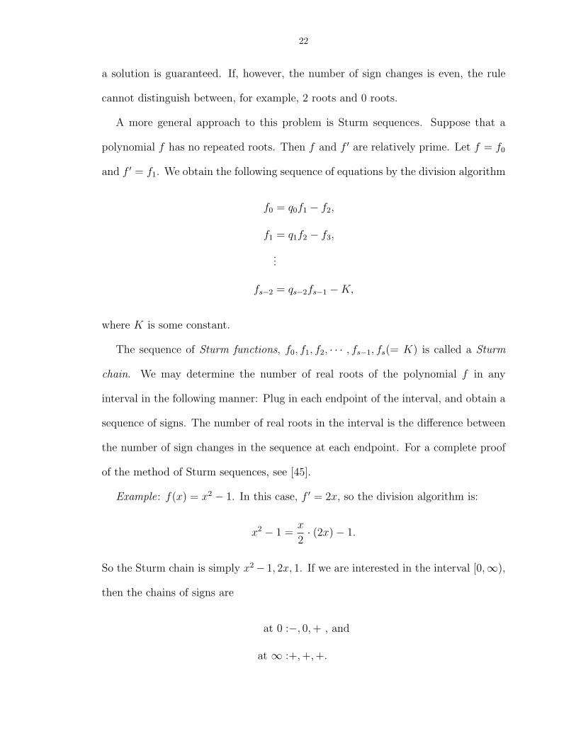
22

a solution is guaranteed. If, however, the number of sign changes is even, the rule

cannot distinguish between, for example, 2 roots and 0 roots.

A more general approach to this problem is Sturm sequences. Suppose that a

polynomial f has no repeated roots. Then f and f ′ are relatively prime. Let f = f0

and f ′ = f1. We obtain the following sequence of equations by the division algorithm

f0 = q0f1 − f2,

f1 = q1f2 − f3,

...

fs−2 = qs−2fs−1 −K,

where K is some constant.

The sequence of Sturm functions, f0, f1, f2, · · · , fs−1, fs(= K) is called a Sturm

chain. We may determine the number of real roots of the polynomial f in any

interval in the following manner: Plug in each endpoint of the interval, and obtain a

sequence of signs. The number of real roots in the interval is the difference between

the number of sign changes in the sequence at each endpoint. For a complete proof

of the method of Sturm sequences, see [45].

Example: f(x) = x2 − 1. In this case, f ′ = 2x, so the division algorithm is:

x2 − 1 =x

2· (2x)− 1.

So the Sturm chain is simply x2− 1, 2x, 1. If we are interested in the interval [0,∞),

then the chains of signs are

at 0 :−, 0,+ , and

at ∞ :+,+,+.

23

There is one sign change in the first sequence and zero in the last, and we conclude

that there is one positive real root to f(x). Similarly, suppose we were interested in

the interval [−2, 2]. Then the sign sequences are

at -2 :+,−,+ , and

at 2 :+,+,+.

There are two sign changes in the first sequence and zero in the second, confirming

that there are two roots in this interval.

Given a specified parameter set, this method gives a simple, implementable algo-

rithm for determining whether a bifurcation occurs, without the need to run the full

simulation of the system of equations for various delays.

2.3 Applications

In [39], we are faced with the characteristic equation

(2.9) λ3 + Aλ2 + (B − δce−λτ )λ+ δcρ− δc(ρ− ψ′)e−λτ = 0,

where A ≡ δ + c + ρ, B ≡ δc + (δ + c)ρ, and ψ′ ≡ ρ − dT > 0, the notation being

that of the paper. In the paper, it is shown that for τ � 1 and τ � 1 no change of

stability occurs. We can extend this result to all τ > 0.

In the notation we have been using, equation (2.9) yields

R1(σ) = −Aσ2 + δcρ,

Q1(σ) = −σ3 +Bσ,

R2(σ) = −δcdT ,

Q2(σ) = −δcσ.

24

Using these specific polynomials, (2.4) becomes

σ6 + (A2 − 2B)σ4 + (B2 − (δc)2 − 2δcρA)σ2 − (δc)2(ψ′2 − 2ρψ′) = 0, or

µ3 + (A2 − 2B)µ2 + (B2 − (δc)2 − 2δcρA)µ− (δc)2(ψ′2 − 2ρψ′) = 0.

(2.10)

This can be simplified by substituting the known values of A, B, and ψ′. For the

µ2 coefficient, we have

A2 − 2B = (δ + c+ ρ)2 − 2(δc+ (δ + c)ρ)

= δ2 + c2 + ρ2 + 2δc+ 2ρc+ 2δρ− 2δc− 2(δ + c)ρ

= δ2 + c2 + ρ2.

Further, for the µ coefficient, we have

B2 − 2δcρA− (δc)2 = ((δc)2 + (δρ)2 + (cρ)2 + 2δ2cρ+ 2δρc2 + 2ρ2δc)

− 2δcρ(ρ+ c+ δ)− (δc)2

= (δρ)2 + (cρ)2.

And for the constant term we have

ψ2 − 2ρψ′ = ψ′(ρ− dT − 2ρ) = −ψ′(ρ+ dT ).

So we may write equation (2.10) as

µ3 + (δ2 + c2 + ρ2)µ2 + ((δρ)2 + (cρ)2)µ+ (δc)2ψ′(ρ+ dT ) = 0.

This is a polynomial with positive coefficients, and cannot have any positive real

roots, therefore the introduction of a delay into the model in Nelson and Perelson

[39] cannot lead to a bifurcation. This is an extension of the results presented in

that paper, where it was proven by asymptotic methods that for very large and very

small delays, the steady state was stable. The argument above shows that this is the

case for all delay lengths.

25

In [38], the following characteristic equation is encountered for a system of delay

differential equations

λ2 + (δ + c)λ+ δc− ηe−λτ = 0,

where δ, c and η are positive constants. We have P1(λ) = λ2 + (δ + c)λ + δc, and

P2(λ) = −η. Thus

R1(σ) = −σ2 + δc,

Q1(σ) = (δ + c)σ,

R2(σ) = −η, and

Q2(σ) = 0.

By the method of the lemma, we arrive at

η2 = (σ2 − δc)2 + (δ + c)2σ2,

η2 = σ4 − 2δcσ2 + δ2c2 + (δ2 + 2δc+ c2)σ2,

0 = σ4 + (δ2 + c2)σ2 + δ2c2 − η2.

(2.11)

Let µ = σ2, then this becomes:

S(µ) ≡ µ2 + (δ2 + c2)µ+ δ2c2 − η2 = 0.

Since the linear coefficient of S is positive, by Descartes’ rule of signs, a positive

real root can occur if and only if the constant coefficient is negative. So a change

of stability occurs if and only if 0 > δ2c2 − η2 = (δc + η)(δc− η), i.e., if and only if

δc < η.

Checking nondegeneracy, we take the derivative of the last line of (2.11), and

check that equality does not hold.

0 = 4(σ∗)3 + 2(δ2 + c2)σ∗, and

0 = 4(σ∗)2 + 2(δ2 + c2),

26

which clearly has no roots. This shows, that a nondegenerate bifurcation does occur

for δc < η. This reproduces the results in Nelson et al [38].

Culshaw and Ruan, in [14] applied this same method to conclude that no bifur-

cations occurred in a delay model with characteristic equation

(2.12) λ3 + a1λ2 + a2λ+ a3e

−λτ + a4λe−λτ + a5 = 0.

In their paper, Culshaw and Ruan follow the method we have presented in Lemma

2, and arrive at the polynomial S if equation (2.5) in the form

z3 + αz2 + βz + γ

Proposition 2 in [14] states that if γ ≥ 0 and β > 0, then this polynomial has no

positive real roots. The proof of this proposition also assumes that α > 0. In this

case all of the coefficients are positive, and there are certainly no positive roots. The

condition α, β, γ > 0 is sufficient, but it is not necessary for no roots to exist. In the

next section we develop a criterion which will extend this result and give necessary

and sufficient conditions for a characteristic equation of the form (2.12) to produce

no bifurcations.

2.4 General Order Two and Three Characteristic Equations

Using Sturm sequences, we can derive some general results for low order char-

acteristic equations. We begin with the general degree two equation, for which a

general result is easy

(2.13) λ2 + aλ+ b+ (cλ+ d)e−λτ = 0.

A steady state with this characteristic is stable for τ = 0 if all of the roots of

λ2 + (a+ c)λ+ (b+ d) = 0

27

have negative real part. By the Routh-Hurwitz conditions, this occurs if and only if

a+ c > 0 and b+ d > 0.

Letting λ = iσ and proceeding as in Lemma 2, we arrive at the following form of

equation (2.5)

(2.14) µ2 + (a2 − c2 − 2b)µ+ (b2 − d2) = 0.

Let A ≡ a2− c2−2b and B ≡ b2−d2. Equation (2.14) has a positive real root in two

circumstances. Since the lead coefficient is positive, if B < 0 then there is a single

positive real root. If B > 0, the roots of (2.14) are

−A±√A2 − 4B

2,

and there is a simple positive root (in fact two simple positive real roots) if and only

if A < 0 and A2 − 4B > 0. Thus we can conclude

Proposition 2.3. A steady state with characteristic equation (2.13) is stable in the

absence of delay, and becomes unstable with increasing delay if and only if

i. a+ c > 0 and b+ d > 0, and

ii. either b2 < d2, or b2 > d2, a2 < c2 + 2b and (a2 − c2 − 2b)2 > 4(b2 − d2).

For similar results in the degree two case, and also for some more general results,

see Kuang [32].

For the degree three problem, the situation is somewhat more complex. The

general characteristic equation is

(2.15) λ3 + a2λ2 + a1λ+ a0 + (b2λ

2 + b1λ+ b0)e−λτ = 0.

The steady state is stable in the absence of delay if the roots of

λ3 + (a2 + b2)λ2 + (a1 + b1)λ+ (a0 + b0) = 0

28

have negative real part. This occurs if and only if a2 + b2 > 0, a0 + b0 > 0 and

(a2 + b2)(a1 + b1)− (a0 + b0) > 0.

In this case the form of equation (2.5) is

(2.16) µ3 + Aµ2 +Bµ+ C = 0,

where

(2.17) A ≡ a22 − b22 − 2a1, B ≡ a2

1 − b21 + 2b2b0 − 2a2a0 and C ≡ a20 − b20.

As in the degree two case, since the lead coefficient is positive, there are two

manners in which a positive real root can occur. The first and simplest is to have

C < 0. Now suppose that C > 0. Since the polynomial is odd, we are guaran-

teed a negative real root. The only way to have a simple positive real root in this

case is to have 2 positive real roots. In other words, all of the roots are real. Now

suppose we take the Sturm chain of the polynomial (2.16), denoted f0, f1, f2, f3.

We evaluate the entire real line, i.e., from −∞ and ∞, and construct a table of the

signs at these endpoints. f0 = µ3+Aµ2+Bµ+C and f1 = 3µ2+2Aµ+B, so we have

-∞ ∞

f0 - +

f1 + +

f2

f3

We know that there must be three real roots. The difference in the number of

sign changes at each endpoint must be three, but this is only possible if the Sturm

sequence at one endpoint is always positive or always negative, and the sequence at

29

the other endpoint must alternate. So the completed table must have the form

-∞ ∞

f0 - +

f1 + +

f2 - +

f3 + +

Notice that f0 and f2 are odd degree polynomials, and f1 and f3 are even degree

polynomials, and the signs at −∞ are the direct consequence of those at∞ (the same

for even polynomials, and the opposite for odd polynomials). Thus, the bifurcation

occurs in the case C > 0 if and only if the lead coefficients f2 and f3 are positive.

Carrying out the division algorithm, the lead coefficient of f2 is

−(2

3B − 2

9A2),

which is positive if and only if A2 − 3B > 0.

f3 is the constant

−9

4

4B3 − A2B2 − 18ABC + 4CA3 + 27C2

(A2 − 3B)2.

After some algebraic manipulation, we can see that this is positive if and only if

(2.18) 4(B2 − 3AC)(A2 − 3B)− (9C − AB)2 > 0.

Now we have conditions to guarantee that there are three real roots. We must

finally guarantee that one of these is positive. This occurs if (2.16) has a positive

critical point. The derivative function is

f1 = 3µ2 + 2Aµ+B,

30

whose roots are −A±√

A2−3B3

. One of these is positive if A < 0 or A > 0 and B < 0,

so either A or B must be negative. So we have

Theorem 2.4. A steady state with characteristic equation (2.15) is stable in the

absence of delay, and becomes unstable with increasing delay if and only if A,B, and

C are not all positive and

i. a2 + b2 > 0, a0 + b0 > 0, (a2 + b2)(a1 + b1)− (a0 + b0) > 0, and

ii. either C < 0, or C > 0, A2−3B > 0 and the condition (2.18) is satisfied, where

A, B and C are given by (2.17).

2.5 Conclusions

So we have developed a method of reducing the question of the existence of a delay-

induced loss of stability to the problem of finding real positive roots of a polynomial.

Although this method has been utilized before, it is useful to see the form of the

polynomials involved. These results are summarized in Lemma 2.2.

The method of this lemma can be used to verify and to extend the results in several

cases from the literature. More generally, it is easy, using the technique, to arrive at

general conditions on the coefficients of a characteristic equation of degree 2, such

that it describes an asymptotically stable steady state which becomes unstable as

the delay parameter is increased. This simple, practical test is given in Proposition

2.3, and is related to analysis done by Y. Kuang in Chapter 3 of his book [32].

The main result of this chapter, presented in Theorem 2.4, is for the degree three

case, where Sturm sequences are used to develop an elementary (though perhaps

algebraically complicated) test for bifurcation. It is hoped that this criterion will

make the investigation of third order systems of delay differential equations simpler,

31

both analytically and numerically. It provides a general algorithm for determining

stability that anyone modeling with delay differential equation models can use.

CHAPTER 3

Single Species Models

In the study of population dynamics, the use of differential equations to study

single species populations is well established. Exponential and logistic growth models

are the most common. We would like to study a class of differential equation models

for a single species that involve a time delay. The goal is to determine whether the

introduction of time delays might enrich the dynamics of these models, or whether

their behavior is essentially the same as the ordinary differential equations models

they modify. In particular, we are interested in determining the existence of periodic

solutions for these models.

In this chapter, I will begin by stating the theorems from functional analysis

which we will use to prove the existence of periodic solutions to the delay differential

equations I will study. This section is followed by the exploration of a model of the

form

(3.1) x(t) = b(x(t− τ))x(t− τ)− d(x(t))x(t),

with b nonincreasing and d nondecreasing, which represents the population dynamics

of a single species with a delayed birth term. Basic properties of this model are

determined, including the types of functions b and d which might lead to the existence

of periodic solutions.

32

33

In the Section 3.3, we specify to the case b(x) = be−ax and d(x) constant. In

this case, I prove the existence of a class of solutions oscillating about the nontrivial

steady state, and then go on to extend a result of Kuang [32], proving the existence

of a periodic solution to this model in a wider parameter set than has previously

been shown.

In Section 3.4, the final one dealing with this model, a delay-dependent term is

added to the parameter b. The effects of this alteration are explored, and conditions

are given for the existence and linear instability of the positive steady state.

Following this, I change the model to make the rate of change proportional to the

current state of the variable, so the model takes the form

(3.2) x(t) = [b(x(t− τ))− d(x(t))]x(t).

The same general plan is followed as with the first model. I begin by exploring the

basic properties of the model, and the forms of b(x) and d(x) which might give rise

to periodic solutions.

In Section 3.6, the case of a constant per capita death rate is explored in detail,

and it is shown that whenever the nontrivial steady state exists and is unstable, a

periodic solutions exists. Finally, we introduce a delay dependence in the parameters

of (3.2), and in the case b(x) = be−ax, I derive the exact range of delays τ for which

a positive periodic solution exists.

3.1 A Fixed-Point Theorem from Nonlinear Functional Analysis

The primary tool available for proving the existence of periodic solutions is the

theorem below from nonlinear functional analysis. Before stating the theorem, we

need to define what it means for a fixed point of a map to be ejective.

34

Definition 3.1. Let X be a Banach space, K a subset of X, and x0 ∈ K. The

point x0 is said to be an ejective point of a map A : X \ {x0} → X if there is an

open neighborhood G ⊂ X of x0 such that, if y ∈ G ∩K, y 6= x0, there is an integer

m = m(y) > 0 such that A(m)(y) /∈ G ∩K.

Intuitively, a point is ejective if it is surrounded by a neighborhood of points,

which the map will sends outside the neighborhood eventually. We now state the

theorem we apply in this chapter and Chapter 4.

Theorem 3.2. If K is a closed, bounded, convex and infinite dimensional set in a

Banach space X, and A : K \ {x0} → K is completely continuous, and x0 ∈ K is

ejective, then there is a fixed point of A in K \ {x0}.

A proof of this theorem is provided by Nussbaum [42]. The primary challenge in

applying this result consists of constructing an appropriate map A. We will show

that solutions of the system oscillate about the nontrivial steady state, and the

“return map” acts on the space of initial functions. A fixed point of this return

map corresponds to a periodic solution, since dictating the behavior of a solution

on an interval of length τ determines all future behavior. Just as with ordinary

differential equations, if an autonomous system returns to its initial condition (or

initial function), it is periodic. This method is analogous to examining a Poincare

map for an ordinary differential equation.

3.2 A General Single-Species Population Model with Delay

The first class of models we will examine will be of the form

(3.3) x(t) = b(x(t− τ))x(t− τ)− d(x(t))x(t).

35

We will consider that b(x) is a continuous, positive, decreasing function, i.e., that the

per capita growth rate of the population decreases with increased population levels.

This is an instance of density-limited growth, of which the logistic model is another

example. The delay in this instance can represent a gestation or maturation period,

so the number of individuals entering the population depends on the levels of the

population at a previous instance of time.

The function d(x) is nondecreasing and positive. This represents the per capita

death rate, which may be increased by intraspecific competition.

Models of this type have been used extensively in the mathematical biology lit-

erature, especially when there is an interest in modelling oscillatory phenomena.

In population biology, for example, [4] and [55] explore the model generally, while

[48] is a specific application to housefly populations. Such models are also used in

other branches of biology, such as physiology [36]. While oscillatory phenomena are

noted, few analytic results about the existence of periodic solutions exist for such

models. One such result is found in [32], Chapter 5, and I will refer to it often.

More commonly, results proving the existence of positive periodic solutions rely on

a non-autonomous periodic forcing term or periodic coefficients, with period greater

than zero ([21], [22], [54]).

Now let us proceed with the analysis by proving the following basic fact.

Lemma 3.3. Given positive initial data, solutions of equation (3.3), where b is a

positive function, remain positive for all time.

Proof. We can simply look at the rate of change by steps. By assumption, x(t) is

positive for t ∈ [−τ, 0], so for t ∈ [0, τ ], it is easy to see that x(t) > −d(x(t))x(t).

So if T ∈ [0, τ ] is the first time at which x(t) = 0, then x(T ) > 0. This is clearly a

36

contradiction, so x(t) > 0 in this interval. Now simply apply the same analysis to

[τ, 2τ ], and so on. So for all t, the solution remains positive.

The requirement that b(x) be positive is necessary, in spite of the analogy to,

for example, the logistic ordinary differential equation. If there is an x such that

b(x) < 0, then there are positive initial histories which become negative. One could

simply set the initial history to be x on [−τ,−ε] for some small ε > 0, and make it

continuous on [−ε, 0] so that x(0) is sufficiently small, say x(0) = −b(x)(τ−ε)x/2 > 0.

One sees that the solution will be driven negative in the interval [0, τ ]. If x(t) ≥ 0

on [0, τ − ε], then

x(τ − ε) ≤ x(0) +

∫ τ−ε

0

b(x(s− τ))x(s− τ)ds

= x(0) +

∫ τ−ε

0

b(x)xds

= −b(x)2

(τ − ε)x+ b(x)(τ − ε)x

=b(x)

2(τ − ε)x < 0,

contradicting the positivity of x(t) on [0, τ − ε).

I will now give three theorems which describe the most general division of possible

behavior regimes for the differential equation (3.3). These results are slightly more

general than the requirement that b be decreasing and d be increasing. Also, it is

likely that these simple results have already been obtained elsewhere, but I have not

seen them recorded. It is useful to see that the case I will consider in detail, that

which will be covered by Theorem 3.4, is the only one with interesting long-term

dynamics.

Theorem 3.4. Consider the delay differential equation (3.3), if b is a positive func-

tion and sup b(x) < inf d(x), then the zero steady state is globally asymptotically

37

stable.

Proof. Let B = sup b(x) and D = inf d(x). We have, then, that x(t) < Bx(t− τ)−

Dx(t), but solutions of y(t) = By(t − τ) − Dy(t) all approach 0 asymptotically as

t→∞, according to Lemma 1.4, since 0 < B < D. So all solutions of (3.3) approach

0 also.

Theorem 3.5. Let b and d be positive functions. Suppose that there exists an x such

that sign(b(x)− d(x)) = −sign(x− x), and b′(x) < d′(x). Then x is a positive steady

state, and the trivial steady state is unstable. If

(3.4) b′(x)x > −2d(x)− d′(x)x,

then x is linearly stable for all τ . Otherwise, there exists a τc > 0 such that x is

stable for τ < τc, and unstable for τ > τc.

Proof. To begin with, x is a unique positive steady state, since b(x)−d(x) = 0 if and

only if x = x. It is the point at which b(x) = d(x). Linearizing about this steady

state yields the equation

(3.5) x(t) = (d(x) + b′(x)x)x(t− τ)− (d(x) + d′(x)x)x(t),

which has characteristic equation

λ = αx(t− τ)− βx(t),

where α = d(x)+ b′(x)x and d(x)+d′(x)x. Since b′(x) < d′(x), α < β. Furthermore,

we know that for |α| < |β| = β, all roots of the characteristic equation have negative

real part. Since α < β, this condition is satisfied if and only if α > −β, but this is

exactly the condition (3.4).

38

If this is not the case, then α < −β. It is clear that for τ = 0, the only char-

acteristic root is λ = α − β < 0. Thus, by the continuity of the location of roots,

for small delays, the system is stable. The derived polynomial for the characteristic

equation is σ− α2− β2, which clearly has a positive real root. Thus there is a τc for

which the characteristic equation has a purely imaginary root. As τ increases past

τc, a root enters the right half-plane. Since the derived polynomial has degree 1, our

Sturm sequence analysis shows that this root can never exit. Thus for τ > τc, the

steady state is unstable.

In [12] the authors prove that if (b(x)x)′ > 0 for all x, then the steady state is

asymptotically stable. A more general result about the linear stability of the model

are also obtained in [12]. These results are contained in Theorem 3.5.

The only situation not covered by the theorems above is when b(x) > d(x) for

all x. In this case, there is no positive steady state, but the trivial steady state is

unstable. This situation is covered by the following theorem.

Theorem 3.6. If

(3.6) limx→∞

b(x) ≥ limx→∞

d(x),

then all solutions of (3.3) with positive initial data are unbounded.

In particular, no positive periodic solutions are possible in this case. We will prove

this theorem via a pair of lemmas.

Lemma 3.7. Given the condition (3.6), a solution, x(t), of equation (3.3) with

positive initial data is bounded if and only if limt→∞ x(t) = 0.

Proof. Since solutions are continuous, it is clear that if x(t) → 0, then it is bounded.

Now suppose that x(t) < M for all t. In this case, define N = b(M)− d(M). Since

39

b is decreasing and d is increasing, we have that b(x(t)) − d(x(t)) ≥ N for all t.

Integrating the differential equation (3.3) yields

x(t) = x(0) +

∫ t

0

[b(x(s− τ))x(s− τ)− d(x(s))x(s)]ds

= x(0) +

∫ 0

−τ

b(x(s))x(s)ds+

∫ t−τ

0

(b(x(s))− d(x(s)))x(s)ds−∫ t

t−τ

d(x(s))x(s)ds.

Define A = x(0) +∫ 0

−τb(x(s))x(s)ds, which is a constant determined by the initial

history of x. Continuing from above, we can find a lower bound on x(t) in the

following manner

x(t) = A+

∫ t−τ

0

(b(x(s))− d(x(s)))x(s)ds−∫ t

t−τ

d(x(s))x(s)ds

≥ A+

∫ t−τ

0

Nx(s)ds−∫ t

t−τ

d(M)Mds

= A− d(M)Mτ +

∫ t−τ

0

Nx(s)ds.(3.7)

Since x(t) < M , the lower bound given by (3.7) must be bounded for all t. In

particular, the integral ∫ ∞

0

Nx(s)ds

must be finite, which implies that x(t) → 0 as t→∞, since x(t) is always positive.

Lemma 3.8. The delay differential equation (3.3), under the conditions of Theorem

3.5 has no solutions which approach 0 as t→∞.

Proof. Given an initial history, we again begin with

x(t) = x(0)+

∫ 0

−τ

b(x(s))x(s)ds+

∫ t−τ

0

(b(x(s))−d(x(s)))x(s)ds−∫ t

t−τ

d(x(s))x(s)ds.

Notice that the first three terms of this expression are positive, and the final term is

the only negative term. Define B =∫ 0

−τb(x(s))x(s)ds. If x(t) → 0, then there exists

40

a T > 0 such that, for all t > T , x(t) < B2d(M)τ

. Where M is an upper bound on x(t).

Now for t > T , ∫ t

t−τ

d(x(s))x(s)ds ≤∫ t

t−τ

d(M)B

2d(M)τds =

B

2.

Thus, for t > T , x(t) > B2, a contradiction.

Given Lemmas 3.7 and 3.8, it is now obvious that solutions with positive initial

data must be unbounded, and thus Theorem 3.6 is proven.

3.3 A Specific Single-Species Delay Model

We will now look specifically at

(3.8) x(t) = bx(t− τ)e−ax(t−τ) − dx(t),

which is a particular case of equation (3.3). We will assume that b > d, so that we

are in the case of Theorem 3.5, where the nontrivial steady state exists.

This particular form of the more general model, with constant per capita death

rate and exponentially decaying per capita birth rate has been used in many models,

for example [4] and [24], especially those dealing with Nicholson’s famous blowfly data

([40], [41]), which sparked much debate about the possibility of chaotic dynamics in

natural populations.

Let us begin by looking at the particulars of this case. The nontrivial steady state

occurs when be−ax = d, i.e., x = 1aln b

d. According to Theorem 3.5 x is stable for all

τ if and only if

d

dxbe−ax

∣∣∣∣x=x

> −2d

x.

This is equivalent to the condition b < de2.

41

Now suppose that b > de2, and let α = ln bd−1. Then α > 1 and the characteristic

equation is

λ = −dαe−λτ − d.

When τ = 0, this is λ = −dα− d. Suppose τ > 0 and that λ = iσ, σ > 0 is a purely

imaginary root. Then the real and imaginary parts of the characteristic equation are

d = −dα cos(στ),

σ = dα sinστ.

Squaring these and summing, we get σ2 + d2 = d2α2, i.e. σ = d(α2 − 1)12 .

Rewriting the real and imaginary parts of the characteristic equation, we see,

cosστ = − 1

α< 0,

sinστ =(α2 − 1)

12

α> 0.

So for τc, the critical delay at which an eigenvalue crosses into the right half-plane,

στc ∈ (π2, π), and the critical delay is

(3.9) τc =1

d(α2 − 1)12

cos−1

(− 1

α

).

For τ > τc the steady state is unstable. From now on, we will assume that b > de2.

3.3.1 Oscillatory Solutions

Now let us take an initial function in the set

K = {φ ∈ C([−τ, 0],R+) : φ(−τ) = x, φ(t) > x, ∀t ∈ (−τ, 0]}.

So long as x(t) > x, a solution to (3.8) with an initial history in K will be decreasing,

since the entire graph of bxe−ax lies below that of dx when x > x (see Figure 3.1).

Let us also define the value xm < x so that xmb(xm) = dx. In the region (xm, x), the

42

entire graph of xb(x) lies above dx, and if a solution remains in this region, then it

must be increasing. We now show that any solution with initial history in K \ {x}

must oscillate about x infinitely often.

x

b(x)x

dx

Figure 3.1: The growth function, b(x)x, and the decay function, dx, intersecting at x

Lemma 3.9. If φ ∈ K, then there exist times 0 < t1 < t2 such that if x(t) is a

solution to (3.8) with initial function φ, then x(t1) = x(t2) = x , x(t1) < 0 and

x(t2) > 0 and x(t) 6= x for any other t ∈ (0, t2)

Proof. Suppose that x(t) > x for all t, then x is monotone decreasing and bounded

below. Thus, x(t) has a limit, and since x must approach 0 as x approaches this

limit, it is clear from the differential equation that x(t) → x.

In order to prove that solutions with initial data in the class K cannot remain

above x and have x as a limit, we must now look more carefully at the critical delay

length τc. We know that the nontrivial steady state is unstable if and only if τ > τc,

43

and we have seen that στc ∈ (π2, π). From the imaginary part of the characteristic

equation when τ = τc, recall that σ = dα sin(στ). We get the following chain of

inequalities, given that the nontrivial steady state is unstable

στ > στc >π

2

τ >π

2

1

dα sin(στ)

>π

2

1

dα>

1

dα.

The form of this inequality we will use is

−dα < −1

τ.

Now consider the function B(x) = xb(x). Taking the derivative at the point

x = x, we get B′(x) = −dα < 0. Note, in particular, that B is decreasing in a

neighborhood of x. For any slope s ∈ (B′(x), 0), there exists a δ > 0 such that for

0 < x− x ≤ δ, B(x)−B(x) < s(x− x). In particular, we now take s = − 1τ.

Let T > τ be a time such that x(T ) = x+ δ. Then for t ∈ [T, T + τ ] we have

x(t) = B(x(t− τ))− d(x(t))

< B(x(t− τ))− dx

< B(x(T ))−B(x)

since x(t) is decreasing for t > 0 and B is decreasing in a neighborhood of x. Also,

B(x) = dx. Continuing,

x(t) < −1

τ(x(T )− x) = − δ

τ

But if x(t) < − δτ

on the interval [T, T + τ ], then x(T + τ) < x(T ) − τ δτ

= x, con-

tradicting the assumption that x(t) remains above x. We are lead to the conclusion

44

that there exists a time t1 such that x(t1) = x, x(t) > x for t ∈ (0, t1), and x(t1) < 0,

as desired.

For t ∈ (t1, t1 + τ), x(t) ≤ x. To see this, suppose that x(t) = x, then x(t) =

x(t− τ)b(x(t− τ))− dx ≥ 0. This implies, x(t− τ)b(x(t− τ)) ≥ dx, but this is not

possible, since at time t − τ , xb(x) is less than dx, as is apparent in the figure 3.1.

Now suppose that x(t) < x for all t > t1. Integrating (3.8), one arrives at

x(t)− x =

∫ t1

t1−τ

f(x(s))x(s)ds+

∫ t−τ

t1

(f(x(s))− d)x(s)ds−∫ t

t−τ

dx(s)ds(3.10)

≥∫ t−τ

t1

(f(x(s))− d)x(s)ds+ A− dτ x,(3.11)

where A is defined to be∫ t1

t1−τf(x(s))x(s)ds, and is fixed by the value of the solution

before entering the region x < x. If the integral∫ t−τ

t1(f(x(s)) − d)x(s)ds fails to

converge, then x(t) → ∞, since the integrand is positive. As this contradicts the

assumption that x(t) < x, we must assume that the integral converges. In particular,

the integrand must approach zero. This can occur if and only if x approaches 0 or

x. We can rule out the case of x(t) → 0 using equation (3.10). As x → 0, the final

term on the right hand side becomes arbitrarily small, and thus x(t)− x > 0. Which

contradicts the assumption that x→ 0.

We conclude that if x(t) < x then x(t) → x. If this is the case, then there exists

a time T so that for x(t) > xm for all t > T , and for these times x(t) is increasing.

The proof that a time t2 exists such that the solution x(t) must increases across

the level x at time t2 is analogous to the proof of the existence of t1, above, and is

omitted.

We are easily led to the following, much more general, result.

Corollary 3.10. Any solution of the delay differential equation (3.8) with positive

initial data is equal to x infinitely often.

45

Proof. If we assume that the solution x(t) satisfies x(t) > x for all t > T , then the

analysis in the proof of the previous theorem derives a contradiction. Similarly, if

x(t) < x for t > T , the previous proof arrives at a contradiction.

3.3.2 An Extension of Previously Known Results

In [32], the author proves the existence of periodic solutions for certain equations

of the form

x(t) = B(x(t− τ))−D(x(t)).

An essential component of this proof, required to guarantee certain properties of the

solution map, was the existence of a value x ∈ (xM , x) such that B(D−1(B(x))) >

D(x). In this section, I provide a broader condition, which not only encompasses a

larger set in the space of parameters, but is also directly verifiable without the need

to find x. The proof of the existence of periodic solutions from [32] will again apply

to this broader case, extending the previous results.

Let B(x) = xb(x), D(x) = xd(x), and let xM be the point at which B achieves

its maximum. Also define xm ∈ (0, xM) such that B(xm) = B(x). If

(3.12) D−1(B(D−1(B(xM)))) > xm,

then the solution operator maps K into K.

Suppose that the initial function φ ∈ K. Then so long as x(t) remains above x,

the solution x(t) is decreasing. As we have seem, the form of the equation dictates

that the solution must cross x at some point t1. For the next τ time units, the value

of B(x(t− τ)) increases, since x(t− τ) decreases, and B is decreasing for x > x.

Claim: x(t) 6= x for t ∈ (t1, t1 + τ).

Proof. If x(t) = x for some t ∈ (t1, t1 +τ), and that t is the smallest such time. Then

46

D(x(t)) = D(x) = B(x) > B(x(t − τ)), and thus x(t) < 0, contradicting the fact

that x(t) < x for t ∈ (t1, t).

So for the interval (t1, t1 + τ), the solution x is below x. We now show for these

times x is above xm. Let us deal with this in two cases: x achieves its minimum at

t1 + τ , and it achieves its minimum at some time in (t1, t1 + τ). The first case is

impossible, since x(t1 + τ) = B(x) − d(x(t)) > B(x) −D(x) = 0. So the minimum

must occur in the interval (t1, t1 + τ). At the minimum,

0 = x(t) = B(x(t− τ))−D(x(t))

D(x(t)) = B(x(t− τ)) ≥ B(D−1(B(xM)))

x(t) ≥ D−1(B(D−1(B(xM)))) > xm.

Thus, in the interval (t1, t1 +τ), the solution x(t) remains in the region (xm, x). In

this region, B(y) > D(x) for all x and y. It follows that x is increasing for t ≥ t1 + τ

for as long as it remains below x. By the same argument as before, the solution must

cross x at some time t2 > t1 + τ . Arguing analogously to the above, since x stays

above xm in the interval (t2 − τ, t2), the maximum of x on the interval (t2, t2 + τ) is

less that F (xM).

Thus, K is mapped into K by the solution operator. Now the arguments from

Kuang apply to show that periodic solutions exist whenever the steady state is

linearly unstable.

For what parameter regimes does the condition (3.12) hold? To begin with, recall

that in our case B(x) = bxe−ax and D(x) = dx. For our functions B and D, the

value of xM can be determined by simply checking where B′(x) = 0. One finds that

xM = 1a. It is much more difficult to determine the value of xm. Rather, we can

find another condition, equivalent to (3.12), which does not require knowledge of the

47

actual value of xm. One has

(3.13) B(D−1(B(D−1(B(xM))))) > B(xm),

since D−1(B(D−1(B(xM)))) ∈ (0, x), and in this region, x > xm is equivalent to

B(x) > B(x) = dx. To apply this condition, one only needs knowledge of B(xm) =

B(x) = daln( b

d).

Now, insert xM = 1a

into (3.13).

b(1

a) =

b

ae−1

D−1(B(1

a)) =

b

ade−1

B(D−1(B(1

a))) =

b2

ade−1e−

bde−1

D−1(B(D−1(B(1

a)))) =

b2

ad2e−1e−

bde−1

B(D−1(B(D−1(B(1

a))))) =

b3

ad2e−1e−

bde−1

e−b2

d2 e−1e−bd

e−1

For the condition to hold, we need the expression above to be greater than B(x) =

daln( b

d). It is clear then that the only truly independent parameter is b

d. In fact, by

rescaling the differential equation, we can assume that the parameter d is equal to

1. We have then

b3

ae−1e−be−1

e−b2e−1e−be−1

>1

aln(b)

b3e−1e−be−1

e−b2e−1e−be−1

> ln(b)

This condition is by no means easy on the eye. We can plot the difference of the left

and right hand sides (see Figure 3.2), and see when the function is positive, in order

to get an idea of the range of the parameter b for which the condition is satisfied.

Recall that we are only interested in b > e2, which is approximately 7.3891.

48

6 8 10 12 14 16 18 20 22

−2

−1.5

−1

−0.5

0

0.5

1

1.5

b

Figure 3.2: The graph of b3e−1e−be−1e−b2e−1e−be−1

− ln(b) against b. When b > e2 and this functionis positive, we can prove the existence of periodic solutions to the delay differentialequation (3.8)

3.4 Delay Dependent Parameters

Staying with the same model as in the previous section, let us examine the effect

of allowing one of the parameters to depend on the length of the delay τ . Specifically,

consider

(3.14) x(t) = be−µτx(t− τ)e−ax(t−τ) − dx(t).

Since the first term in this equation represents recruitment or birth rate, the mod-

ification of this parameter could represent the decreased survivorship over a longer

incubation or maturation time. I will examine the effect of this delay dependence on

the existence and stability of the nontrivial steady state.

The mathematical difficulty imposed by this alteration is twofold. First of all, the

location of the steady state will now vary with the length of the delay. Secondly,

49

the form of the characteristic equation will change due to the direct inclusion of the

delay in the parameters, and the indirect changes resulting from the varying location

of the steady state.

Let us begin by locating the steady states of the model (3.14). The zero steady

state still exists, and a nontrivial steady state is given by

be−µτe−ax = d

which leads to

x =1

aln

b

deµτ

In particular, if τ > 1µ

ln bd, there is no positive steady state. In this case, given

positive initial data, we have

x(t) ≤ be−µτy(t− τ)− dy(t),

with be−µτ < d, so the solution goes to 0, and the trivial steady state is globally

stable.

Now we examine the characteristic equation for the positive steady state, given

a particular delay τ < 1µ

ln bd. We linearize the equation (3.14) as usual, and assume

an exponential solution to get the new characteristic equation

(3.15) λ = −dα(τ)e−λτ − d,

where α(τ) = 1− ln bdeµτ .

This characteristic equation is essentially the same as that for the delay-independent

case; only α(τ) is affected. In the case of delay-independent parameters, we found a

critical time delay τc, given in equation (3.9), such that the characteristic equation

λ = −dαe−λτ − d

50

has a root with positive real part if and only if τ > τc. We will now use this result

to get the condition for instability of (3.14).

Theorem 3.11. The nontrivial steady state of the delay differential equation (3.14)

is unstable if and only if

(3.16) τ >1

d(α(τ)2 − 1)12

cos−1

(− 1

α(τ)

).

Notice in particular that this condition includes the requirement that α(τ)2−1 >

0, which is equivalent to ln bdeµτ (ln b

deµτ − 2) > 0. This is equivalent to the condition

that be−µτ > de2, similar to the condition b > de2, which needed to be satisfied in

order for a change of stability to occur in the delay-independent case. So we have

Theorem 3.12. The positive steady state of (3.14) exists and is unstable if and only

if τ < 1µ

ln bd, and inequality (3.16) is satisfied. In this case, all solutions with positive

initial data oscillate about the steady state.

3.5 Another General Model

Now let us turn our attention to a slightly different model formulation.

(3.17) x(t) = (b(x(t− τ))− d(x(t)))x(t),

where b and d are again decreasing and increasing, respectively. As opposed to the

model in equation 3.3, in this model, only the nonlinear components of the birth term

are delayed. This could be thought of to correspond to a delayed density dependence

in the per capita birth rate. The delayed logistic models is a particular example

of (3.17). Dynamics of this form often form part of predator-prey and food chain

models, for example [37].

51

The conditions for the existence of a positive steady state are the same as before,

but the linearizations are different. As before, we have the following two results,

which are included for completeness, in spite of their simplicity.

Theorem 3.13. If b(0) < d(0), then the delay differential equation (3.17) has no

positive steady state, and the trivial steady state is globally asymptotically stable.

Proof. It is clear that x(t) ≤ (b(0) − d(0))x(t), and so solutions to the full delay

differential equation are bounded by x(0)e(b(0)−d(0))t, which approaches 0 as t →

∞.

Theorem 3.14. If

limx→∞

b(x) > limx→∞

d(x),

in equation (3.17), then any solution with positive initial history approaches ∞ as

t→∞

Proof. It is clear in this case that the graph of maxx≥0 d(x) < minx≥0 b(x), so x(t)

is positive for all t. If such an increasing solution is bounded, then it has a limit

L > 0, but this would imply 0 = limt→∞ x(t) = (b(L) − d(L))L, which is clearly

impossible.

The most interesting case of this model is, however, when the graphs of b and d

intersect, so that there is a nontrivial steady state. In contrast to the model (3.3), in

this case the nontrivial steady state does not always change stability. Let x(t) ≡ x be

the unique positive steady state of this delay differential equation, i.e. b(x) = d(x).

Then the linearization of the equation about this steady state is

(3.18) x(t) = b′(x)xx(t− τ)− d′(x)xx(t),

52

and the characteristic equation is

(3.19) λ = −ae−λτ − b,

where we define

a = −b′(x)x > 0, and

b = d′(x)x > 0.

When the delay τ is sufficiently small, this characteristic equation has only roots

with negative real part, and the steady state is stable. For some parameter regimes,

however, longer delays result in an unstable steady state. These results are summa-

rized in the following theorem.

Theorem 3.15. If d′(x) > −b′(x), then the nontrivial steady state x is linearly stable

for all τ . For d′(x) < −b′(x), there exists a τc such that for τ < τc, the steady state

is stable, and for τ > τc, it is unstable.

Proof. We have the characteristic equation (3.19). Write λ = µ + iσ, and we can

separate this equation into its real and imaginary parts, yielding

µ+ b = −ae−µτ cos(στ)(3.20)

σ = ae−µτ sin(στ).(3.21)

If b > a and µ ≥ 0, then the magnitude of the left hand side of the real part (3.20)

is always strictly greater than the magnitude of the right hand side. Thus only roots

with negative real part exist, for all τ . This proves the first part of the theorem.

Now suppose a > b. It is clear that when τ = 0, the steady state is stable

(λ = −a − b < 0). We use the method described in Chapter 2. The derived

polynomial equation in this case is σ2 + b2−a2 = 0. This has a solution if and only if

53

a > b. Since there is only one possible imaginary root, once a root passes to the right

half plane, further increases in τ cannot remove it, so the steady state is unstable

for all τ > τc. This completes the proof of the second part.

3.6 Constant per capita Death Rates

Now let us specify to the case of d(x) = d, a constant, so that we have the

differential equation

(3.22) x(t) = (b(x(t− τ))− d)x(t).

We will focus on the interesting case, where b(0) > d, b is decreasing and b(x) = d

for some unique x. For this case, we prove that this system has periodic orbits when

the nontrivial steady state is unstable.

Let us begin with the linear stability analysis. The nontrivial steady state, x

exists, and the linearization at this point is

(3.23) x(t) = b′(x)xx(t− τ).

This leads to the characteristic equation

(3.24) λ = −βe−λτ ,

where β = −b′(x)x > 0. Note that when τ = 0, the steady state is stable, as the

characteristic equation has exactly one root, which is negative. If we separate the

components of the eigenvalue as λ = µ + iσ, then the real and imaginary parts of

the characteristic equation are

µ = −βe−µτ cos(στ),(3.25)

σ = βe−µτ sin(στ).(3.26)

54

Now suppose that (3.24) has a purely imaginary root, λ = iσ. The equation becomes,

0 = −β cos(στ),(3.27)

σ = β sin(στ).(3.28)

We are looking for the smallest positive value of τ such that there is a solution

σ > 0. From the real part (3.27), we see that στ = π2

is the smallest possible value

for this product. Using this information in the imaginary part (3.28) we see that

σ = β = −b′(x)x. So we see that the critical delay τc at which the first eigenvalue

with positive real part emerges is τc = π2σ

, i.e.,

(3.29) τc =−π

2b′(x)x,

and for τ > τc, the nontrivial steady state x is unstable.

Any characteristic root of (3.24) with positive real part is also simple. If not, then

we must have

λ = −βe−λτ ,(3.30)

1 = βτe−λτ .(3.31)

Substituting the first formula in the second gives

(3.32) 1 = −τλ,

and it is clear that is Re(λ) > 0, then equation (3.32) cannot be.

Let us take the time now to record a couple of facts which we will refer to in

proving later results. If we choose the delay τ such that the steady state is unstable,

then b′(x) < −π2xτ

. Furthermore, when µ > 0, cos(στ) < 0 (from equation (3.25)) and

sin(στ) > 0, when we consider the complex root with nonnegative imaginary part.

So στ ∈ (π2, π).

55

Lemma 3.16. Suppose that x(t) is a solution of equation (3.22), x(t0) = x, and

x(t) < x for all t ∈ [t0 − τ, t0]. Then for all t > t0, x(t) < xe(b(0)−d))τ = M .

Proof. The function x(t) is increasing for t ∈ [t0, t0 + τ ], since b(x(t − τ)) > d for

these times. Since b(x) is a decreasing function, x(t) ≤ (b(0) − d)x(t), so it is clear

that x(t0 + τ) ≤ M . For t ∈ [t0 + τ, t0 + 2τ ], b(x(t − τ)) < d, so x(t) is decreasing.

If x(t) remains above x for all t ≥ t0, then it is always decreasing, and x(t) < M,∀t.

Otherwise, there is a time, t1 such that x(t1) = x. In this case, x(t) decreases on

the interval [t1, t1 + τ ]. If x(t) now remains below x for t > t1, then we are done.

Otherwise, there is a time t2 such that x(t2) = x. We have returned to the situation

of the lemma. So we have proven that such solutions either oscillate about x with

x(t) < M , or else are eventually monotone (in which case x(t) → x).

The final preparatory definition we require is of a subset, K ⊂ C([−τ, 0],R+) of

the Banach space of initial functions.

K = {φ ∈ C([−τ, 0],R+) : φ(−τ) = x, φ nondecreasing, and φ(0) ≤M}.

We will show that for any solution x(t) with initial function φ ∈ K1 = K \{x}, there

is a time t = t(φ) such that x(t+ s) is in K1.

Theorem 3.17. Suppose that φ ∈ K1, and that x(t) is the solution to the differential

equation (3.22) with initial function φ. Then there exists a time t1 such that x(t1) =

x, and x(t1) < 0. Further, there exists a time t2 > t1 + τ such that x(t2) = x and

x(t2) > 0. If t = t2 + τ , then the function defined by x(t + s) for −τ ≤ s ≤ 0 is in

K1.

Proof. Suppose that t1 does not exist, then for t > 0, x(t) is decreasing and bounded

below by x. It follows that x(t) approaches a limit L as t→∞. This is only possible

56

if L = x. Since b′(x) < −π2xτ

, for any α < π2, it is true that

b(x)− b(x) ≤ − α

τx(x− x),

for x such that |x− x| < δ′ = δ′(α). In particular, this is true for α = 1. See Figure

(3.3) for an illustration of this fact. Choose δ < min{x(τ), δ′(1)}. For x− x > δ,

b(x)

(π/2τ x*)(x−x*)+d

(1/τ x*)(x−x*)+d

Figure 3.3: The function b(x), its tangent, and a line with slope greater than the tangent

b(x)− d < b(x+ δ)− d < − 1

τ xδ,

since b(x) = d.

Now let T be a time such that x(T ) = x + δ. Due to the definition of δ, T > τ ,

and x(t) > x+ δ for t ∈ [T − τ, T ). Then for t ∈ [T, T + τ ], we have

x(t) = (b(x(t− τ))− d)x(t)

≤ (b(x(t− τ))− d)x

≤ − 1

τ xδx = − δ

τ.

57

Now x(T + τ) < x(T )− δττ = x(T )− δ = x, which is a contradiction.

We have shown that any solution with initial history in K1 must cross the non-

trivial steady state, at a time which we call t1. From this crossing time, the solution

continues to decrease for exactly τ units of time, and then begins to increase. We

now show that the solution must reach the nontrivial steady state again. Essentially

the same analysis works are before, now we have

b(x)− b(x) ≥ − 1

τ x(x− x) =

1

τ x(x− x).

From this point on, the work is analogous, with the directions of the inequalities

reversed.

The next order of business is to show that the steady state x is an ejective fixed

point to the return map. To do this we follow a method described in Kuang [32]

(Section 2.9) and proven by Chow and Hale [9]. If we consider the linearized equation

x(t) = −βx(t− τ),

then for any eigenvalue λ, there is a decomposition of the space of initial functions

C([−τ, 0],R+) = Pλ ⊕ Qλ into subspaces invariant under the solution operator, and

Pλ is the generalized eigenspace of eigenvalue λ. Let πλ be the projection onto Pλ.

Rather than proving it directly from the definition, we will use the following theorem

to show that the steady state x is ejective.

Theorem 3.18. Suppose that the following conditions are satisfied:

1. There is a characteristic root λ with Re(λ) > 0.

2. There is a closed convex set K, x ∈ K and δ > 0 so that

inf{||πλ(φ)|| : φ ∈ K, ||φ|| = δ} > 0,

and

58

3. There is a completely continuous function τ : K \ {x} → [α,∞), α ≥ 0 such

that the map defined by

Aφ = xτ(φ)(φ), φ ∈ K \ {x},

takes K \ {x} into K and is completely continuous.

Then x is ejective.

Since the eigenvalue λ is simple, Pλ is a one dimensional space. We define

φ1(θ) =1

1 + λτeλθ = γeλθ, for θ ∈ [−τ, 0]

ψ(s) = e−λs, for s ∈ [0, τ ],

Φ1 = (φ1, φ1),

Ψ = (ψ, ψ).

For the linear operator L in (3.23) and φ ∈ K1 we define a measure η(θ), by

L(f) = −βφ(−τ) =

∫ 0

−τ

dη(θ)φ(θ)

η(−τ) = 0, η(θ) = −β, for θ ∈ (−τ, 0]

We now compute the bilinear form

(ψ, φ1) = ψ(0)φ1(0)−∫ 0

−τ

∫ θ

0

ψ(ξ − θ)φ1(ξ)dξdη(θ)

= γ +

∫ 0

−τ

∫ ξ

−τ

ψ(ξ − θ)φ1(ξ)dη(θ)dξ

= γ −∫ 0

−τ

βψ(ξ + τ)φ1(ξ)dξ

= γ − γβ

∫ 0

−τ

e−(ξ+τ)λeλξdξ

= γ(1− βτe−λτ ) = γ(1 + λτ) = 1.

59

Also, we have

1

γ(ψ, φ1) = 1− β

∫ 0

−τ

e−λ(ξ+τ)eλξdξ

= 1− βe−λτ

[1

λ− λe(λ−λ)ξ

]0

−τ

= 1− β1

λ− λ(e−λτ − e−λτ )

=1

λ− λ(λ+ βe−λτ − (λ+ βe−λτ )) = 0.

From these two computations, it follows readily that (ψ, φ1) = 0 and (ψ, φ1) = 1.

So, (Ψ,Φ1) is the identity, so for any φ ∈ C([−τ, 0],R+), πλφ = Φ1(Ψ, φ). So we need

to show that

inf{||(ψ, φ− x)|| : φ ∈ K1, ||φ− x|| = δ} > 0.

Let λ = µiσ, and recall that µ > 0, στ ∈ (π2, π). We can compute the coefficient

(ψ, φ− x), and split it into its real and imaginary parts, yielding

Real part: φ(0)− x− β

∫ 0

−τ

e−µ(ξ+τ)(φ(ξ)− x) cos(ξ + τ)σdξ(3.33)

Imaginary part: β

∫ 0

−τ

e−µ(ξ+τ)(φ(ξ)− x) sin(ξ + τ)σdξ(3.34)

If the infimum is 0, then there is a sequence φn ∈ K1 with ||φn − x|| = δ, and

both the real and imaginary parts above go to zero. For the given range of σ and

ξ, sin(ξ + τ)σ > 0 and bounded away from 0 when ξ is near 0. Further, φn − x is

increasing, so the integral in (3.34) can only go to zero only if ||φn − x|| → 0, which

is a contradiction. Thus the fixed point x is ejective, and we can apply the Theorem

(3.2). This system has periodic solutions when the steady state is unstable.

3.7 Delay Dependent Parameters

60

0 5 10 15 20 25 30 35 400

50

100

150

t

x(t)

0 5 10 15 20 25 30 35 4020

22

24

26

28

t

x(t)

Figure 3.4: Solutions of the x(t) = (be−ax(t−τ) − d)x(t), with a = 0.1, b = 10, d = 1, with initialfunction x + 10t on [−τ, 0]. τc = 0.6822. The upper graph is for τ = 1, and the secondfor τ = 0.5.

As in section 3.4, we will now examine the effects of allowing a parameter in the

equation (3.22) depend on the delay, τ . We will use the same type of dependence,

so that we are interested in

(3.35) x(t) = (e−µτb(x(t− τ))− d)x(t).

This form of the delay model allows us to obtain much more explicit results than

were possible in Section 3.4. The location of the nontrivial steady state is now the

value x, for which

b(x) = deµτ ,

and since b is decreasing, the x is no longer biologically meaningful if b(0) < deµτ .

Thus as τ increases, the nontrivial steady state will disappear.

61

The characteristic equation for (3.35) is

λ = e−µτb′(x)xe−λτ ,

which is similar in form to the characteristic equation (3.24) for the delay-independent

case. We can use the analysis use in the previous section to prove the following result.

Theorem 3.19. If

(3.36)πeµτ

−2b′(x)x< τ <

1

µlog

b(0)

d,

then the nontrivial steady state of (3.35) exists and is unstable. Furthermore, there

exist positive, periodic solutions of this differential equation.

It must be remembered that x is a decreasing function of τ . The first inequality

in (3.36) is the condition for instability, obtained from our calculations of the critical

delay, τc, in the delay-independent case. The second inequality is the condition for

the positivity of the nontrivial steady state.

If we specify to the case where b(x) = be−ax, as we have considered previously,

then the picture becomes remarkably clear. In this case, b′(x) = −ab(x) = −adeµτ ,

b(0) = b, and x = 1aln b

deµτ . Thus the condition for the instability of the steady state

(3.36) becomes

τ >π

−2adx

=π

2d ln bde−µτ

=π

2d

1

ln bd− µτ

.

This becomes the quadratic equation in τ ,

µτ 2 − τ lnb

d+

π

2d< 0,

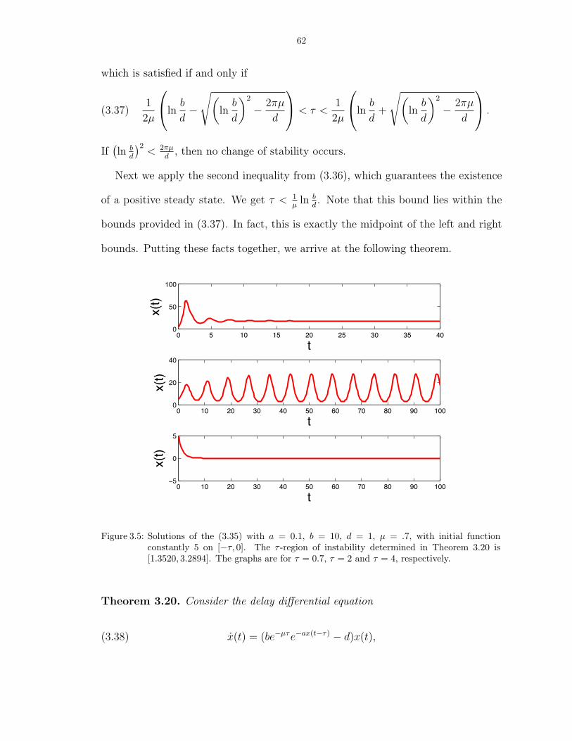
62

which is satisfied if and only if

(3.37)1

2µ

lnb

d−

√(lnb

d

)2

− 2πµ

d

< τ <1

2µ

lnb

d+

√(lnb

d

)2

− 2πµ

d

.

If(ln b

d

)2< 2πµ

d, then no change of stability occurs.

Next we apply the second inequality from (3.36), which guarantees the existence

of a positive steady state. We get τ < 1µ

ln bd. Note that this bound lies within the

bounds provided in (3.37). In fact, this is exactly the midpoint of the left and right

bounds. Putting these facts together, we arrive at the following theorem.

0 5 10 15 20 25 30 35 400

50

100

t

x(t)

0 10 20 30 40 50 60 70 80 90 1000

20

40

t

x(t)

0 10 20 30 40 50 60 70 80 90 100−5

0

5

t

x(t)

Figure 3.5: Solutions of the (3.35) with a = 0.1, b = 10, d = 1, µ = .7, with initial functionconstantly 5 on [−τ, 0]. The τ -region of instability determined in Theorem 3.20 is[1.3520, 3.2894]. The graphs are for τ = 0.7, τ = 2 and τ = 4, respectively.

Theorem 3.20. Consider the delay differential equation

(3.38) x(t) = (be−µτe−ax(t−τ) − d)x(t),

63

with b > d. If (lnb

d

)2

<2πµ

d,

then the nontrivial steady state is stable for all delays τ for which it exists. Otherwise,

for

1

2µ

lnb

d−

√(lnb

d

)2

− 2πµ

d

< τ <1

µlnb

d,

the nontrivial steady state is unstable, and positive periodic solutions exist. For

smaller τ , the nontrivial steady state is stable, and for larger τ , it is no longer

positive, and the zero steady state is globally stable.

CHAPTER 4

Predator-Prey Interaction Models

4.1 The Lotka-Volterra Predator-Prey Interaction Model

One of the most universally recognized models in mathematics is the classic model

for the interaction of a single predator species and a single prey specie developed by

Alfred Lotka [34] and Vito Volterra [53]. If we let x represent the prey species, and

we let y represent the predator species, then the model has the form,

x(t) = ax− bxy

y(t) = cxy − dy,

(4.1)

where a, b, c and d are positive constants. We see that this model includes an expo-

nential growth term for prey in the absence of predation, and an exponential decay

for predators in the absence of prey. The interaction of the two species is represented

by a mass action term, which implicitly assumes that the two species encounter each

other at a rate proportional to each population level, and that the effect of predation

on each is in turn proportional to the number of encounters.

This system of two ordinary differential equations has two steady state solutions,

(0, 0) and (dc, a

b). It is well known that the trivial steady state is a saddle, while the

nontrivial steady state is a center, and solutions in the phase plane form an infinite

family of periodic orbits (Figure 4.1).

64

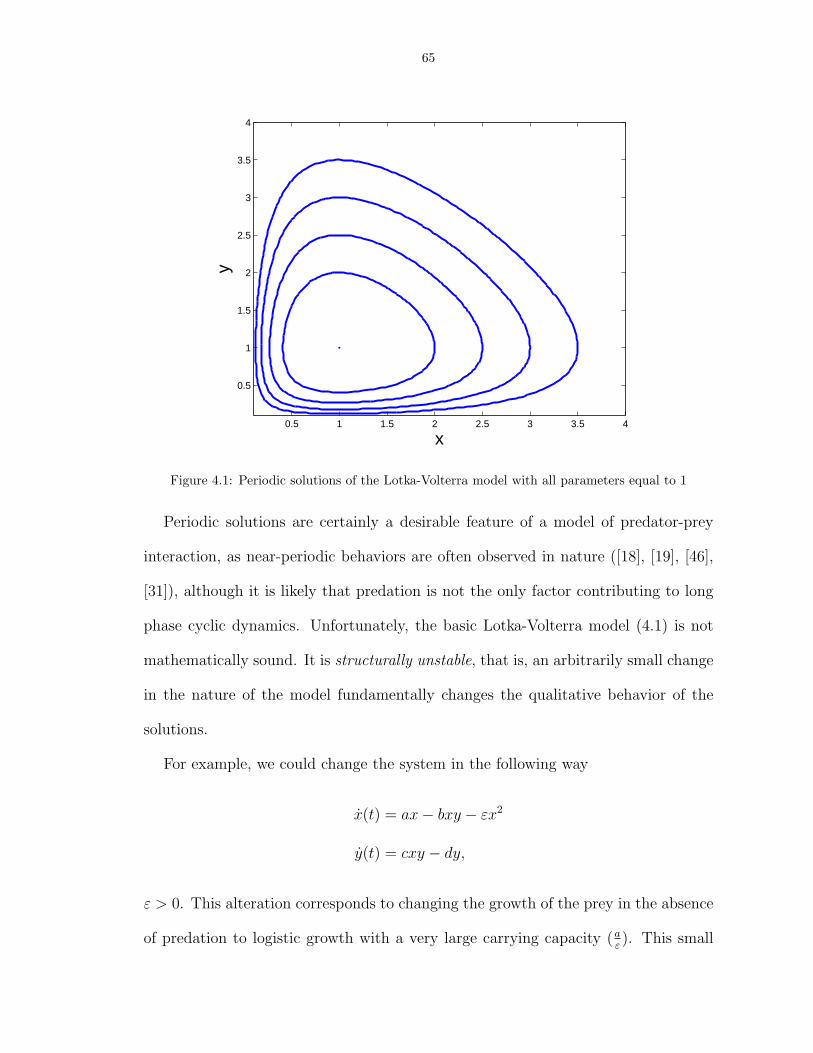
65

x

y

0.5 1 1.5 2 2.5 3 3.5 4

0.5

1

1.5

2

2.5

3

3.5

4

Figure 4.1: Periodic solutions of the Lotka-Volterra model with all parameters equal to 1

Periodic solutions are certainly a desirable feature of a model of predator-prey

interaction, as near-periodic behaviors are often observed in nature ([18], [19], [46],

[31]), although it is likely that predation is not the only factor contributing to long

phase cyclic dynamics. Unfortunately, the basic Lotka-Volterra model (4.1) is not

mathematically sound. It is structurally unstable, that is, an arbitrarily small change

in the nature of the model fundamentally changes the qualitative behavior of the

solutions.

For example, we could change the system in the following way

x(t) = ax− bxy − εx2

y(t) = cxy − dy,

ε > 0. This alteration corresponds to changing the growth of the prey in the absence

of predation to logistic growth with a very large carrying capacity (aε). This small

66

change in the nature of the model completely alters the nature of the phase portrait

of the models. The infinite family of periodic orbits is lost and replaced by solutions

which all approach the nontrivial steady state (Figure 4.2).

0 0.5 1 1.5 2 2.5 3 3.50

0.5

1

1.5

2

2.5

x

y

Figure 4.2: Solutions to the perturbed Lotka-Volterra model, ε = .2, a = b = c = d = 1

There are several possible ways of making the Lotka-Volterra system more palat-

able mathematically and biologically, each leading to interesting modelling questions

and mathematical results. To begin with, we will retain the logistic growth term for

the prey population in the absence of predation. Ideally, we will develop a model

which corresponds well with biologically observed behavior regimes, including some

kind of periodic behavior or sustained oscillation, and which is mathematically ro-

bust.

One option is to include stochastic effects in the model. This can often lead to

sustained oscillations due to the constant perturbation of the system. While this is

an intriguing option, it is beyond the scope of my current research.

67

Another option is to choose more robust nonlinearities in the predation term.

While mass action is reasonable, it is not the only possibility. If we write the preda-

tion term as p(x)y, p(x) is known as the functional response, and is a quantification

of the relative responsiveness of the predation rate to changes in prey density at

various population levels of prey. Kot [30] and Begon [1] describe four categories

of functional response encountered in the ecological literature ([25], [26], [27], [28],

[13]). Type I is the standard mass action or linear response

p(x) = cx.

Type II is the so-called Monod response

p(x) =cx

a+ x,

which is hyperbolic, with a saturation level (c) due to the time it takes to handle

prey. Type III is a sigmoidal response

p(x) =cx2

a2 + x2,

which includes the feature that predators are inefficient when prey levels are low.

These three types of functional response are all increasing functions of the prey

population x. A Type IV response includes a decrease at large population levels,

corresponding to prey group defenses or toxicity to predators. In the following, we

will consider functional responses of Types I-III.

Thirdly, one may alter the Lotka-Volterra model by including a delay. A delay

takes into account the non-instantaneous nature of biological processes. Statistical

evidence has been reported ([49], [50]) of delayed effects in the density dependence

of the growth rate of several insect and plant species. Another possibility for the

inclusion of delays is in the interaction term p(x)y. This would represent the time

68

necessary to convert prey biomass into predator biomass, for instance due to gestation

periods or time required for maturation. Some ecologists have also suggested that

the inclusion of a delay could help to explain certain phenomena observed in long

population cycles [5]. The inclusion of delays make the analysis of these models more

difficult, but also broadens the spectrum of possible behavior regimes.

4.2 A Delay Model of Predator-Prey Interaction

We will look at a system with three populations, x is the prey population, y

represents mature predators, and yj is the juvenile predator population, which does

not hunt.

dx

dt= rx(1− x

K)− yp(x)(4.2)

dy

dt= be−djτy(t− τ)p(x(t− τ))− dy(t)(4.3)

dyj

dt= by(t)p(x(t))− be−djτy(t− τ)p(x(t− τ))− djyj(t)(4.4)

Let us look at the third equation in more detail. Consumed prey are converted to

juvenile (immature) predator instantly with a conversion rate b. They remain in this

stage of development for τ units of time, decaying exponentially at rate dj. After

this time, the survivors are removed to the class of mature predators y. It is easy to

see that the third equation can be decoupled from the others, as the quantity yj does

not appear in either of the first two equations. This gives a system of two equations,

and a change of variables simplifies things as well, so that we are left with

x(t) = x(1− x)− yp(x)

y(t) = be−djτy(t− τ)p(x(t− τ))− dy.

(4.5)

The function p(x) represents the adult predators functional response to prey, and

we make the following assumptions

69

• p(0) = 0, i.e., no predation occurs in the absence of prey,

• p is increasing,

• p(x)/x is bounded and not 0 at x = 0.

These requirements include function responses of types I, II and III, but not IV, as

the latter violate the second requirement.

The most important feature of the model is the term

p(x(t− τ))y(t− τ),

with the delay in both state variables. Due to this, the dydt

is no longer proportional

to y(t), the current state of the system. If the delay were omitted from y(t), the

behavior of this system would be much simpler to understand. Biologically, however,

this type of nonlinear inclusion of the delay is entirely natural, and more logical than

including the delay only in the x term. In fact, this type of term is common in

delayed infection disease models [14], [39].

4.3 Preliminary Analysis

We begin by establishing some basic properties of solutions to the system (4.5).

• Given positive initial data, solutions remain positive for all time.

• Solutions are bounded (in fact, eventually uniformly bounded regardless of ini-

tial data).

• Thirdly, we need to determine steady states and their stability.

– The non-trivial steady state becomes unstable for larger delays.

– Periodic solutions exist.

70

4.3.1 Positivity of Solutions

It is relatively easy to establish that solutions remain positive for all times, given

a bounded positive initial history on an interval [a − τ, a]. For y, on the interval

[a, a + τ ], we have y(t) ≥ −dy(t). Thus it is clear that y must remain positive.

Further, y remains finite on this interval. If M is the bound on x(t) on [a − τ, a],

then y(t) ≤ be−djτy(t− τ)p(M)− dy(t), which implies

y(t)− dy(t) = be−djτy(t− τ)p(x(t− τ))

d

dt(e−dty(t)) = be−dte−djτy(t− τ)p(x(t− τ))

Integrating both sides from a to a+ ε, ε ∈ [0, τ ], yields

e−d(ε+a)y(a+ ε) = e−day(a) +

∫ a+ε

a

be−dse−djτy(s− τ)p(x(s− τ))ds

y(a+ ε) = edεy(a) +

∫ a+ε

a

bed(ε+a−s)e−djτy(s− τ)p(x(s− τ))ds.

The right hand side is finite for ε ∈ [0, τ ], since the integrand is also bounded.

For the prey population, the rate of change is essentially proportional to x

x = x(1− x− yp(x)

x).

The state variable x can only become negative if 1 − x − y p(x)x

becomes infinite

and negative as x → 0, but the function p(x)x

is bounded, and y is bounded for

t ∈ [a, a + τ ]. It follows that x cannot become negative on this interval. We may

iterate this argument to show that x and y are positive and finite for all t ≥ a− τ .

4.3.2 Uniform Boundedness of Solutions

Next we show that all solutions of (4.5) are eventually in a fixed region.

71

Theorem 4.1. There exists an M > 0 such that for any solution (x(t), y(t)) of the

system (4.5) with positive initial data,

max

{lim sup

t→∞x(t), lim sup

t→∞y(t)

}≤M.

Proof. Since p is a positive function for x > 0, and solutions remain positive for all

t, we have x(t) ≤ x(t)(1 − x(t)). Prey solutions of (4.5) with positive initial data

are thus given an upper bound by solutions of z(t) = z(1 − z) with positive initial

conditions. All such solutions converge to 1, so we can conclude that lim supt→∞ x(t)

is given an upper bound by 1, regardless of initial data.

Now consider the second equation of (4.5). Suppose that be−djτp(1)− d < 0 (we

shall see that this is the condition of nonexistence of a nontrivial steady state). There

exists an ε > 0 such that be−djτp(1 + ε) − d < 0, due to the continuity of p. Since

lim supt→∞ x(t) ≤ 1, there exists a T1 such that x(t) < 1 + ε for all t > T1 − τ . This

T1 will depend on the particular solution (i.e., initial data), but the bound provided

for lim supt→∞ y(t) will not depend on T1. For t > T1, we have

y(t) = be−djτp(x(t− τ))y(t− τ)− d(y)

≤ be−djτp(1 + ε)y(t− τ)− dy(t)

= ay(t− τ)− dy(t),

where we define a = be−djτp(1 + ε) < d. We have seen in Lemma 1.4 that solutions

of

z(t) = az(t− τ)− dz(t)

approach 0 as t → ∞. Further, the comparison lemma 1.5 now tells us that y(t) is

bounded by z, and thus goes to 0 as well. Clearly, then lim supt→∞ y(t) = 0 in this

case.

72

We are left with the case be−djτ ≥ d. Since 1 is a bound on lim supt→∞ x(t), for a

particular solution, there exists a time T2 such that x(t) < 2 for all t ≥ T2. Thus

(4.6) y(t) ≤ be−djτp(2)y(t− τ)− dy(t).

Looking at the equation for y again, we have y(t) ≥ −dy(t). From this, one easily

concludes that for t2 > t1,

y(t2) ≥ y(t1)ed(t2−t1).

In particular, let t2 = t > τ and t1 = t − τ , and one obtains y(t − τ) ≤ y(t)edτ .

Combining this information with equation (4.6) yields

y(t) ≤ (be−djτp(2)edτ − d)y(t)

= ∆y(t),

defining ∆ by this second equality. Now for t2 > t1, y(t2) < y(t1)e∆(t2−t1), and this

implies

(4.7) t2 − t1 ≥1

∆lny(t2)

y(t1).

Define p1(x) by p(x) = xp1(x). By our assumptions about p, we know that p1 is

bounded, positive and bounded away from 0 for x ≥ 0. Suppose that there exists a

time T3 such that p1(x(t))y(t) > 1 for all t ≥ T3. Then for t ≥ T3,

x(t) = x(t)(1− x(t)− p1(x(t))y(t)) ≤ −x(t)2.

Solutions to the differential x = −x2 tend uniformly to zero, so for any z0 > 0, there

exists a time T4 > τ such that x(t) < z0 for all t > T2 + T3 + T4. In particular,

we shall consider the case of z0 such that be−djτp(z0) < de−dτ < d. This yields the

estimate of the rate of change of y

y ≤ ay(t− τ)− dy(t),

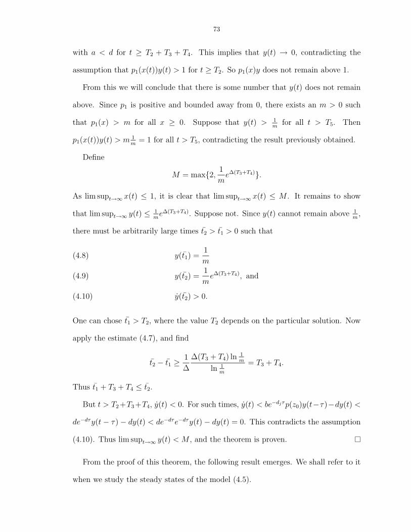
73

with a < d for t ≥ T2 + T3 + T4. This implies that y(t) → 0, contradicting the

assumption that p1(x(t))y(t) > 1 for t ≥ T2. So p1(x)y does not remain above 1.

From this we will conclude that there is some number that y(t) does not remain

above. Since p1 is positive and bounded away from 0, there exists an m > 0 such

that p1(x) > m for all x ≥ 0. Suppose that y(t) > 1m

for all t > T5. Then

p1(x(t))y(t) > m 1m

= 1 for all t > T5, contradicting the result previously obtained.

Define

M = max{2, 1

me∆(T3+T4)}.

As lim supt→∞ x(t) ≤ 1, it is clear that lim supt→∞ x(t) ≤ M . It remains to show

that lim supt→∞ y(t) ≤ 1me∆(T3+T4). Suppose not. Since y(t) cannot remain above 1

m,

there must be arbitrarily large times t2 > t1 > 0 such that

y(t1) =1

m(4.8)

y(t2) =1

me∆(T3+T4), and(4.9)

y(t2) > 0.(4.10)

One can chose t1 > T2, where the value T2 depends on the particular solution. Now

apply the estimate (4.7), and find

t2 − t1 ≥1

∆

∆(T3 + T4) ln 1m

ln 1m

= T3 + T4.

Thus t1 + T3 + T4 ≤ t2.

But t > T2+T3+T4, y(t) < 0. For such times, y(t) < be−djτp(z0)y(t−τ)−dy(t) <

de−dτy(t− τ)− dy(t) < de−dτe−dτy(t)− dy(t) = 0. This contradicts the assumption

(4.10). Thus lim supt→∞ y(t) < M , and the theorem is proven.

From the proof of this theorem, the following result emerges. We shall refer to it

when we study the steady states of the model (4.5).

74

Corollary 4.2. When be−djτp(1)−d < 0, solutions to (4.5) with positive initial data

satisfy

limt→∞

(x(t), y(t)) = (1, 0).

Proof. As we have seen in the previous proof, when be−djτp(1)−d < 0, lim supt→∞ y(t) =

0. Due to the positivity of solutions, this is equivalent to limt→∞ y(t) = 0. Re-

call also that lim supt→∞ x(t) ≤ 1. Thus, for ε > 0 there exists a time T such

that for t ≥ T , x(t) < 1 + ε, and, possibly by increasing T , one can assume that

p(x(t))y(t) < p(1 + ε)y(t) < ε. Now for t > T , if x(t) > 1, then

x(t) = x(t)(1− x(t))− p(x(t))y(t) < (1 + ε)(1− x(t)) < 0.

So x is decreasing. On the other hand, if x(t) < 1, then

x(t) = x(t)(1− x(t))− p(x(t))y(t) > x(t)(1− (1− ε))− ε = −ε(x(t)− 1) > 0

for t > T . So, in this case, x is increasing. It follows immediately that for t > T , x(t)

cannot cross x = 1, and is monotone. A limit must therefore exist, and x(t) → 1 is

the only possibility.

4.3.3 Steady States

To determine the steady states of the system (4.5), we simply assume that a

constant (x, y) is a solution and determine what these contant values must be. The

equations for determining steady states are

0 = x(1− x− yp(x)

x)(4.11)

0 = be−djτp(x)y − dy.(4.12)

75

If y = 0, then the second equation is satisfied, and the first gives (0, 0) and (1, 0)

as steady states.

If y 6= 0, then the steady state equations become

0 = 1− x− yp(x)

x(4.13)

d = be−djτp(x).(4.14)

For the equation (4.13), we must clearly have x ∈ (0, 1). Since p is an increasing

function, it is clear that the second equation has a solution if and only if

(4.15) p(1) >d

be−djτ.

So, if the condition (4.15) is satisfied, the system (4.5) has three steady state so-

lutions: (0, 0), (1, 0), and a nontrivial steady state (x∗, y∗). If (4.15) is not satisfied,

then only the first two steady states exist. Note, in particular, that as the length,

τ , of the delay is increased, this condition will eventually fail, due to the rational

function on the left hand side of (4.15).

4.3.4 Linear Stability

The linearization of the delayed Lotka-Volterra system (4.5) about the steady

state (0, 0) is x

y

=

1 0

0 −d

x

y

+

0 0

0 0

xτ

yτ

,

where xτ = x(t− τ), and similarly for y. This linear system clearly has eigenvalues

1 and −d, and is thus a saddle.

The linearization about the steady state (1, 0) is −1 −p(1)

0 −d

x

y

+

0 0

0 be−djτp(1)

xτ

yτ

.

76

The characteristic equation is

(4.16) (λ+ 1)(λ+ d− be−djτp(1)e−λτ ).

We will now see that the stability or instability of the steady state (1, 0) corre-

sponds exactly to the nonexistence or existence of the nontrivial steady state. Clearly,

λ = −1 is an eigenvalue, but has no bearing on linear stability. The stability of this

steady state therefore depends on the location of the roots of

(4.17) λ+ d− be−djτp(1)e−λτ = 0.

Recall that the condition for the existence of a nontrivial steady state is d <

be−djτp(1). In this case, if we rewrite the characteristic equations as

λ = be−djτp(1)e−λτ − d,

then the left hand side is 0 when λ = 0 and increases to infinity, and the left hand

side is positive when λ = 0, and decreases to 0. Therefore, we see that there is always

a positive real eigenvalue when the nontrivial steady state exists.

When the nontrivial steady state does not exist (i.e., d ≥ be−djτp(1)) we can show

that there are no eigenvalues with positive real part. Setting λ = µ+ iσ, with µ > 0,

the real part of the characteristic equation is

0 = µ+ d− be−djτp(1)e−µτ cos(στ)

≥ µ+ d− be−djτp(1) > 0

So the steady state (1, 0) is stable in the absence of the nontrivial steady state. In

fact, it we have already shown in Corollary 4.2 that in this case, (1, 0) is globally

stable, as demonstrated in Figure 4.3

77

0 0.5 10

0.5

1

1.5

x(t)

y(t)

Figure 4.3: Global stability of (1,0) in the absence of a nontrivial steady state

When the nontrivial steady state does exist, i.e., when d < be−djτp(1), (1, 0) is

always unstable. In fact, in this case the characteristic equation always has a real,

positive root. To see this consider, as before,

λ = be−djτp(1)e−λτ − d.

When λ = 0, the left hand side is zero, while the right hand side is positive. As

λ increases along the real line, the left hand side increases to infinity, while the

right hand side decreases to −d. Since the functions on the left and right sides are

continuous, they must intersect, proving the existence of a positive real eigenvalue.

The linear stability picture for the nontrivial steady state, (x∗, y∗) is more com-

plicated. If we take p(x) = px, then we can show that for small delays, the steady

state in stable.

P (λ, τ) +Q(λ, τ)e−(λ+dj)τ ,

78

where

P (λ, τ) = λ2 + (2x∗ + y∗p′(x∗)− 1 + d)λ+ d(2x∗ + y∗p′(x∗)− 1)

= (λ+ 2x∗ + y∗p′(x∗)− 1)(λ+ d)

Q(λ, τ) = p(x∗)λ− bp(x∗)(2x∗ − 1)

= p(x∗)(λ− b(2x∗ − 1))

We treat the length of delay, τ , as a bifurcation parameter. One should note, in

particular, that the coefficients of these polynomials depend on the location of the

steady state (x∗, y∗), which, in turn, depends on τ . When the parameters of the

model are independent of delay, i.e., dj = 0, the location of this steady state is fixed,

we may refer to the general criteria for determining whether delay induced instability

occurs, which were developed earlier (Chapter 2, also [20]).

When parameters depend on delay, no such criteria exist. Using methods which

depend in an essential manner on numerical estimations [3], Gourley and Kuang [23]

determined that there is a range of delays for which the nontrivial steady state exists

and is unstable. In this case, all steady states are unstable, and all solution are

eventually trapped in a fixed region. One is naturally led to consider the possibility

of periodic solutions.

4.4 Existence of Periodic Solution

The goal of my work on this two dimensional system has been to make progress

toward a proof of the following conjecture.

79

Conjecture 4.3. For the system

x(t) = x(1− x)− yp(x),

y(t) = be−djτy(t− τ)p(x(t− τ))− dy,

if the non-trivial steady state exists and is unstable, then a positive, nonconstant

periodic solution exists.

Numerical simulations give some hope that this result might hold. If we arrange

the parameters so that the nontrivial steady state exists in the absence of delay, then

for small delays, this steady state is globally stable (Figure 4.4).

0 0.1 0.2 0.30

1

2

3

4

x(t)

y(t)

τ=0.1,φ(t)=(.3,1) for −τ≤ t≤ 0

Figure 4.4: Global stability of (x∗, y∗) for small delays

As the delay is increased, a stable limit cycle appears to emerge (Figure 4.5).

For certain parameter regimes, however, the behavior of solutions appears chaotic

(Figures 4.6,4.7).

80

0 0.1 0.2 0.3 0.4 0.5 0.6 0.7 0.80

0.5

1

1.5

2

2.5

3A sample orbit, delayed LK system, unstable s.s.

x

y

Figure 4.5: Emergence of a stable limit cycle

4.4.1 The “Phase Plane”

If we plot y against x, then we get the “phase plane”, where it is easier to see the

interaction of the two population levels. In particular, it is useful to divide the x-y

plane into the following regions,

R1 = {(x, y) : x ≤ 0, f(x, y) ≥ 0}

R2 = {(x, y) : x ≤ 0, f(x, y) ≤ 0}

R3 = {(x, y) : x ≥ 0, f(x, y) ≤ 0}

R4 = {(x, y) : x ≥ 0, f(x, y) ≥ 0},

where f(x, y) is defined by x = −p(x)f(x, y), i.e., f(x, y) = y − x(1−x)p(x)

.

This division of the phase plane is depicted in Figure 4.8. It should be noted that

only the curve Γ is a true nullcline (in this case for x). When solutions are above

81

0 0.1 0.2 0.3 0.4 0.5 0.6 0.7 0.8 0.9 10

0.2

0.4

0.6

0.8

1

1.2

1.4

x(t)

y(t)

Figure 4.6: Chaotic solutions in the phase plane

this curve, x is decreasing, and when below, x is increasing. The vertical line x = x∗

is included only for reference. Due to the delays involved in the rate of change of y,

no meaningful nullcline can be drawn.

Furthermore, this is not a phase plane in the traditional sense; solutions can

cross each other, or even themselves. This possibility is demonstrated in Figure

4.6. Due to this complication, we cannot apply such geometrically-based results

as Poincare-Bendixson and Bendixson-Dulac to prove the existence or otherwise of

periodic solutions. We expect from the phase plane depicted in Figure 4.8 that

solutions will oscillate in a counterclockwise direction, but this behavior is much

trickier to prove than in the case of ordinary differential equations.

4.4.2 Oscillation of Solutions

82

400 450 500 550 600 650 700 750 8000

0.2

0.4

0.6

0.8

1

t

x(t)

400 450 500 550 600 650 700 750 8000

0.2

0.4

0.6

0.8

1

1.2

1.4

t

y(t)

Figure 4.7: Time series for a chaotic solution

As a first step in showing that solutions do indeed oscillate about the steady state

when it is unstable, we show that if the x component of solutions remain eventually

above or below x = x∗, they must approach the steady state. This result is contained

in the following theorems

Theorem 4.4. If there exists a T such that x(t) < x∗ for all t > T , then (x(t), y(t)) →

(x∗, y∗) as t→∞.

Proof. We begin with the differential equation for y(t)

y(t) = be−djτy(t− τ)p(x(t− τ))− dy(t).

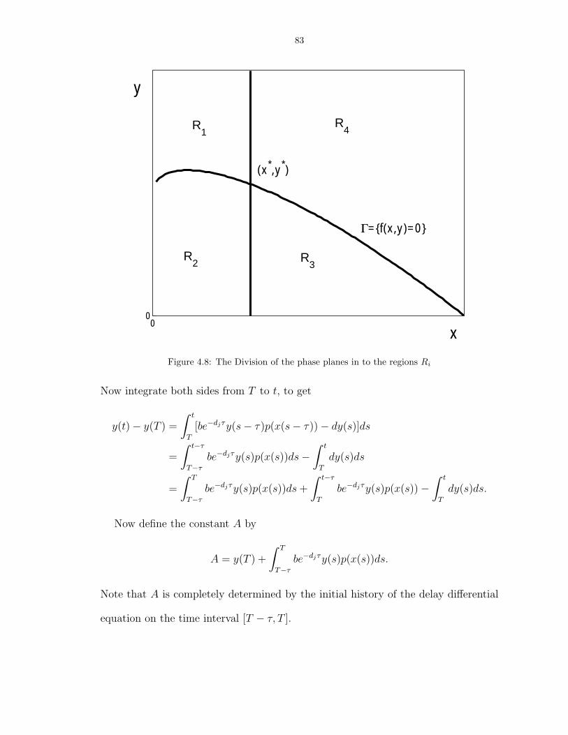
83

00

x

y

Γ={f(x,y)=0}

R4 R

1

R2 R

3

(x*,y*)

Figure 4.8: The Division of the phase planes in to the regions Ri

Now integrate both sides from T to t, to get

y(t)− y(T ) =

∫ t

T

[be−djτy(s− τ)p(x(s− τ))− dy(s)]ds

=

∫ t−τ

T−τ

be−djτy(s)p(x(s))ds−∫ t

T

dy(s)ds

=

∫ T

T−τ

be−djτy(s)p(x(s))ds+

∫ t−τ

T

be−djτy(s)p(x(s))−∫ t

T

dy(s)ds.

Now define the constant A by

A = y(T ) +

∫ T

T−τ

be−djτy(s)p(x(s))ds.

Note that A is completely determined by the initial history of the delay differential

equation on the time interval [T − τ, T ].

84

From the above equation, we can derive two inequalities. First, we have

y(t) ≤ A+

∫ t

T

be−djτy(s)p(x(s))−∫ t

T

dy(s)ds(4.18)

= A−∫ t

T

(d− be−djτp(x(s)))y(s)ds.(4.19)

We shall now use this bound on y to see that x(t) → x∗ under the hypothesis of

this theorem.

We begin with the case x(t) < x∗, i.e., be−djτp(x(t)) < d, and consider the

inequality (4.19) The integrand is positive, so the integral is increasing with t. Since

y(t) is known to be positive, we must have∫ ∞

T

(d− be−djτp(x(s)))y(s)ds <∞,

and the continuity of the integrand then allows us to conclude that

(d− be−djτp(x(t)))y(t) → 0,

as t→∞. One may not immediately conclude that either of the terms of this product

approaches 0, but we will show that indeed, d−be−djτp(x(t)) must approach 0, which

is to say, that x→ x∗.

To see this, consider the times t1, t2, · · · at which x(t) has a relative minimum.

It is obvious that these times can only occur when the solution crosses the curve Γ.

In the region where x < x∗, the y values of the curve Γ are bounded below by some

non-zero m. Thus (d − be−djτp(x(ti)))y(ti) ≥ (d − be−djτp(x(ti)))m ≥ 0. Since the

left-hand side goes to 0, the right hand side must do so as well. But this is only

possible if be−djτp(x(ti)) → d, i.e., x(ti) → x∗, and if the relative minima approach

x∗, then it is simple to see that x(t) → x∗.

If x → x∗, then x → 0, and we can see from the differential equation for x that

y(t) → y∗. This proves the theorem for the first case.

85

We can prove the same result in the case that x(t) > x∗. Before doing so, we need

to establish the following lemma.

Lemma 4.5. If x(t) > x∗ for t > T , and the initial history of x and y are positive,

then y is bounded away from 0 for t > T .

Proof. For positive initial data, it has already been shown in [23] we have already

seen that solutions are positive. We deal with two cases: y has finite number of

relative minima, and y has an infinite number relative minima.

In the first case, if y(t) is not bounded away from 0, then y(t) → 0, and there

exists a T2 > T such that y(t) < 0 for all t > T2. So for t > T2 + τ

0 > be−djτp(x(t− τ))y(t− τ)− dy(t)

y(t) >be−djτp(x(t− τ))

dy(t− τ) ≥ y(t− τ)

which contradicts the assumption that y(t) is decreasing.

For the second case, consider the times t1 < t2 < t3 < · · · at which y(t) has a

relative minimum. At such times we have y(ti) = 0, i.e.

y(ti) =be−djτp(x(ti − τ))

dy(ti − τ) ≥ y(ti − τ) ≥ y(tj)

for some j < i. We can continue thus until we arrive at y(t) for some t ∈ [T − τ, T ],

and thus

` = mint∈[T−τ,T ]

y(t) > 0

is a positive lower bound of y(t) with t > T .

Theorem 4.6. If there exists a T such that x(t) > x∗ for t > T , then (x(t), y(t)) →

(x∗, y∗) as t→∞.

86

Proof. Let M be an upper bound on y(t). We begin as before with

y(t) = A+

∫ t−τ

T

be−djτy(s)p(x(s))ds−∫ t

T

dy(s)ds(4.20)

= A+

∫ t−τ

T

(be−djτp(x(s))− d)y(s)ds− d

∫ t

t−τ

y(s)ds(4.21)

≥ A+

∫ t−τ

T

(be−djτp(x(s))− d)y(s)ds− dMτ.(4.22)

The function y(t) is bounded above, so the lower bound given by (4.22) must

remain finite as t→∞. As in the proof of the previous theorem, since the integrand

is positive, we must have (bedjτp(x(t)) − d)y(t) → 0, but Lemma 4.5 proves that

y is bounded away from 0 under the hypotheses of the theorem. It follows that,

be−djτp(x(t))−d→ 0, and as in the previous theorem, this implies that (x(t), y(t)) →

(x∗, y∗).

Now, when we choose τ large enough that the nontrivial steady state (x∗, y∗) is

unstable, it remains to derive a contradiction from this limiting behavior. Given such

a contradiction, we conclude that x(t) is not less than x∗ for all t, and the solution

curve must leave the region R1 ∪R2. The only possibility for this to occur is for the

curve to pass from region R2 to region R3 at a point with y < y∗. This is clear since

x is decreasing when the solution is above the curve Γ.

We have shown the following,

Theorem 4.7. If there exists a T such that x(t) < x∗ or x(t) > x∗ for all t > T ,

then

(x(t), y(t)) → (x∗, y∗)

as t→∞.

4.5 Future Work

87

Although much has been done to better our understanding of this system, much

work remains. To begin with, a contradiction must be derived to the possibility of a

solution approaching the linearly unstable nontrivial steady state as t→∞. Barring

this, some other argument must be made to guarantee that solutions cross into the

region R3. Once this is accomplished a similar argument will provide the desired

return map.

More generally, there are qualitative questions to answer about the nature of the

solution space for this model. For example, are multiple periodic solutions possible?

Also, when nontrivial periodic solutions do exist, what are their stability properties?

Numerical evidence (for example Figures 4.6 and 4.7) suggests the existence of chaotic

solution regimes. What conditions lead to this behavior for solutions?

Finally, how are these dynamics changed when the system is expanded to include

more equations? Such systems can be used as models for food chains. Even in

the case of ordinary differential equations, food chain systems based on the same

principles as Lotka-Volterra predator prey systems can display a wide variety of dy-

namics. Understanding the delay models could provide more insight into the nature

of such systems, or demonstrate that such models are inappropriate for modeling

such biological situations.

CHAPTER 5

Conclusion

The use of delay differential equations in the modeling of biological phenomena

has become more prevalent in recent years. Analytic results about the behavior of

such models is still largely lacking. While numerical simulations provide a basic

understanding of these systems, and allow, for example, the use of parameter fit-

ting, even when analytic results are unavailable. To be sure, increased computation

capacity and speed make the use of such simulations easier. A better analytic un-

derstanding of these models, however, would make the use of numerics even more

useful, and help in the selection of appropriate models in the first place.

The methods of Chapter 2 provide a straightforward and easily applicable method

for analyzing the linear stability of the steady states of such models. The later chap-

ters focused on showing the existence of periodic solutions. The methods for ap-

proaching such questions remain quite cumbersome. Ideally, a better understanding

of the functional analytic theorems at work here would lead to easier determination

of the existence or otherwise of periodic solutions, at least in the case of a system

of only two differential equations. For ordinary differential equations, one has theo-

rems such as Poincare-Bendixson which allow one to draw conclusions based solely

on global properties (the existence of a trapping region) and linear instability. I

88

89

hope that continued study of the question of periodicity will lead to steps in the

direction of such theorems for delay models. At the very least, a simpler method of

determining the ejectivity of a fixed point would be quite welcome.

I have spent much time in this thesis attempting to determine the properties

of delay differential equations models. I have mentioned that understanding these

properties would make it easier to determine the appropriateness of these models for

biological phenomena. Much work remains to be done on this question. Although

it seems intuitively clear that delays occur in nature, and that they might therefore

play a significant role in the dynamics of a given system, the models I have studied

are only first approximations. All of the models studied incorporate a discrete delay.

In other words, the dynamics depend on the current state of the system and the state

of the system exactly τ time units ago. This way of including the delay requires much

refinement.

Consider the example of human pregnancy. The gestation period is generally

stated to be nine months, but this is hardly exact. If such a reproductive delay

is significant in the dynamics of some model, then surely the variation about the

mean delay time will also be significant. Discrete delays are only an approximation.

These systems ought to be studied, since the chance of obtaining concrete results is

greater for discrete delays than for their distributed cousins, and knowledge of their

behavior provides insight into more complete, distributed models. One suspects that

the behavior of the discrete model should correspond to the expected behavior, for

example, of a stochastic model, where the length of delay is determined by a proba-

bility distribution function. If discrete delay models are to serve as approximations,

however, it will be important to determine the extent to which their behavior is an

artifact of the essentially discontinuous inclusion of past data.

90

As biologists turn to mathematics to provide a framework for understanding more

and more complicated phenomena, it is important to have as many modeling tech-

niques as possible available for use. While the inclusion of delays is but one approach

among many, the theory behind it should continue to be developed, with an eye es-

pecially toward practical results and the ability to draw applicable conclusions.

BIBLIOGRAPHY

91

92

BIBLIOGRAPHY

[1] M. Begon and M. Mortimer. Population Ecology. Blackwell Scientific Publications, Oxford,1981.

[2] R. Bellman and K. L. Cooke. Differential-Difference Equations. Academic Press, New York,1963.

[3] E. Beretta and Y. Kuang. Geometric stability switch criteria in delay differential systems withdelay dependent parameters. SIAM J. Math. Anal., 33(5):1144–1165, 2002.

[4] S.P. Blythe. Instability and complex dynamic behaviour in population models with long timedelays. Theor. Pop. Biol., 22:147–176, 1982.

[5] R. Boonstra, C.J. Krebs, and N.C. Stenseth. Population cycles in small mammals: The prob-lem of explaining the low phase. Ecology, 79:1479–1488, 1998.

[6] T.A. Burton. Stability and Periodic Solutions of Ordinary and Functional Differential Equa-tions. Academic Press, New York, 1985.

[7] S. A. Campbell, R. Edwards, and P. van den Driessche. Delayed coupling between two neuralnetwork loops. SIAM J. Appl. Math., 65(1):316–335, 2004.

[8] N. G. Chebotarev and N. N. Meiman. The Routh-Hurwitz problem for polynomials and entirefunctions. Trudy Mat. Inst. Steklov., 26, 1949.

[9] S.-N. Chow and J. K. Hale. Periodic solutions of autonomous equations. J. Math. Anal. Appl.,66:495–506, 1978.

[10] S. M. Ciupe, B. L. de Bivort, D. M. Bortz, and P. W. Nelson. Estimates of kinetic parametersfrom HIV patient data during primary infection through the eyes of three different models.Math. Biosci. in press.

[11] K. Cooke, Y. Kuang, and B. Li. Analyses of an antiviral immune response model with timedelays. Canad. Appl. Math. Quart., 6(4):321–354, 1998.

[12] K. L. Cooke, P. van den Driessche, and X. Zou. Interaction of maturation delay and nonlinearbirth in population and epidemic models. J. Math. Biol., 39:332–352, 1999.

[13] M. J. Crawley. Natural Enemies: The Population Biology of Predators, Parasites and Disease.Blackwell Scientific Publications, Oxford, 92.

[14] R. V. Culshaw and S. Ruan. A delay-differential equation model of HIV infection of CD4+T-cells. Math. Biosci., 165:27–39, 2000.

[15] R. D. Driver. Ordinary and Delay Differential Equations. Springer-Verlag, New York, 1977.

[16] L. Edelstein-Keshet. Mathematical Models in Biology. McGraw-Hill, New York, 1988.

[17] L.E. El’sgol’ts and S.B. Norkin. An Introduction to the Theory and Application of DifferentialEquations with Deviating Arguments. Academic Press, New York, 1973.

93

[18] J.P. Finerty. The Population Ecology of Cycles in Small Mammals. Yale University Press,New Haven, 1980.

[19] J.R. Flowerdew. Mammals: Their Reproductive Biology and Population Ecology. EdwardArnold, London, 1987.

[20] J. Forde and P. W. Nelson. Applications of Sturm sequences to bifurcation analysis of delaydifferential equation models. J. Math. Anal. Appl., 300:273–284, 2004.

[21] H. I. Freedman and J. H. Wu. Periodic solutions of single species models with periodic delay.SIAM J. Math. Anal., 23:689–701, 1992.

[22] H. I. Freedman and H. X. Xia. Periodic solutions of single species models with delay. Differ-ential Equations, Dynamical Systems and Control Science, pages 55–74, 1994.

[23] S. A. Gourley and Y. Kuang. A stage structured predator-prey model and its dependence onmaturation delay and death rate. J. Math. Biol., 49:188–200, 2004.

[24] W. S. C. Gurney, S. P. Blythe, and R. M. Nisbet. Nicholson’s blowfly revisited. Nature(London), 287:17–21, 1980.

[25] C. S. Holling. The characteristics of simple types of predation and parasitism. Can. Entomol.,91:385–398, 1959.

[26] C. S. Holling. The components of predation as revealed by the study of small mammal preda-tion of the European pine sawfly. Can. Entomol., 91:293–320, 1959.

[27] C. S. Holling. The functional response of predators to prey density and its role in mimicry andpopulation regulation. Mem. Entomol. Soc. Can., 45:1–60, 1965.

[28] C. S. Holling. The functional response of invertebrate predators to prey density. Mem. Ento-mol. Soc. Can., 47:2–86, 1966.

[29] E.I. Jury and M. Mansour. Positivity and nonnegativity conditions of a quartic equation andrelated problems. IEEE, Transactions on Automatic Control, 26:444–451, 1981.

[30] M. Kot. Elements of Mathematical Ecology. Cambridge University Press, Cambridge, 2001.

[31] C.J. Krebs, S. Boutin, R. Boonstra, A.R.E. Sinclair, J.N.M. Smith, M.R.T. Dale, K. Martin,and R. Turkington. Impact of food and predation on the snowshoe hare cycle. Science,269:1112–1115, 1995.

[32] Y. Kuang. Delay Differential Equations with Applications to Population Biology. AcademicPress, New York, 1993.

[33] M. S. Lee and C.S. Hsu. On the τ -decomposition method of stability analysis for retardeddynamical systems. SIAM J. of Control, 7:242–59, 1969.

[34] A. Lotka. Elements of Physical Biology. Williams and Wilkins, Baltimore, 1925.

[35] N. MacDonald. Biological Delay Systems: Linear Stability Theory. Cambridge UniversityPress, Cambridge, 1989.

[36] M. C. Mackey and L. Glass. Oscillation and chaos in physiological control systems. Science,197:287–289, 1977.

[37] R.M. May. Stability and Complexity in Model Ecosystems. Princeton University Press, Prince-ton, 1974.

[38] P. W. Nelson, J. D. Murray, and A. S. Perelson. A model of HIV-1 pathogenesis that includesan intracellular delay. Math. Biosci., 163:201–215, 2000.

94

[39] P. W. Nelson and A. S. Perelson. Mathematical analysis of delay differential equation modelsof HIV-1 infection. Math. Biosci., 179:73–94, 2002.

[40] A.J. Nicholson. An outline of the dynamics of animal populations. Aust. J. Zool., 2:9–65,1954.

[41] A.J. Nicholson. The self adjustment of populations of change. Cold Spring Harb. Symp. quant.Biol., 22:153–173, 1957.

[42] R. D. Nussbaum. Periodic solutions to some nonlinear autonomous functional differentialequations. Ann. Mat. Pura Appl. (4), 101:263–306, 1974.

[43] L. S. Pontriagin. On the zeros of some elementary transcendental functions. Izv. Acad. NaukSSSR, 6(3):115–134, 1942.

[44] M. M. Postnikov. Stable polynomials. Nauka, 1982.

[45] A. Prestel and C. N. Delzell. Positive Polynomials: from Hilbert’s 17th problem to real algebra.Springer-Verlag, Berlin, 2001.

[46] A.R.E. Sinclair, D. Chitty, C.I. Stefan, and C.J. Krebs. Mammal population cycles: evidencefor intrinsic differences during snowshoe hare cycles. Can. J. Zool./Rev. Can. Zool., 81:216–220, 2003.

[47] P. Smolen, D. Baxter, and J. Byrne. A reduced model clarifies the role of feedback loops andtime delays in the Drosophila circadian oscillator. Biophys. J., 83:2349–2359, 2002.

[48] C. E. Taylor and R. R. Sokal. Oscillation in housefly populations due to time lag. Ecology,57:1060–1067, 1976.

[49] P. Turchin. Rarity of density dependence or population regulation with lags. Nature, 344:660–663, 1990.

[50] P. Turchin and A. D. Taylor. Complex dynamics in ecological time series. Ecology, 73:289–305,1992.

[51] B. Vielle and G. Chauvet. Delay equation analysis of human respiratory stability. Math.Biosci., 152(2):105–122, 1998.

[52] M. Villasana and A. Radunskaya. A delay differential equation model for tumor growth. J.Math. Biol., 47(3):270–294, 2003.

[53] V. Volterra. Varizioni e fluttuazioni del numero d’individui in specie animali conviventi. Mem.R. Acad. Naz. dei Lincei (ser. 6), 2:31–113, 1926.

[54] W. Wang, P. Fergola, and C. Tenneriello. Global attractivity of periodic solutions of populationmodels. J. Math. Anal. Appl., 211:498–511, 1997.

[55] P.J. Wangersky and W. J. Cunningham. On time lags in equations of growth. Proc. Nat.Acad. Sci. USA, 42:699–702, 1956.

[56] T. Zhao. Global periodic solutions for a differential delay system modeling a microbial popu-lation in the chemostat. J. Math. Anal. Appl., 193:329–352, 1995.

ABSTRACT

Delay Differential Equation Models in Mathematical Biology

by

Jonathan Erwin Forde

Chair: Patrick W. Nelson

In this dissertation, delay differential equation models from mathematical biology

are studied, focusing on population ecology. In order to even begin a study of such

models, one must be able to determine the linear stability of their steady states, a

task made more difficult by their infinite dimensional nature. In Chapter 2, I have

developed a method of reducing such questions to the problem of determining the

existence or otherwise of positive real roots of a real polynomial. The method of

Sturm sequences is then used to make this determination. In particular, I devel-

oped general necessary and sufficient conditions for the existence of delay-induced

instability in systems of two or three first order delay differential equations. These

conditions depend only on the parameters of the system, and can be easily checked,

avoiding the necessity of simulations in these cases.

With this tool in hand, I begin studying delay differential equations for single

species, extending previously obtained results about the existence of periodic solu-

1

tions, and developing a proof for a previously unproven case. Due to the infinite

dimensional nature of these equations, it is quite difficult to prove the existence of

periodic solutions. Nonetheless, knowledge of their existence is essential if one is to

make decisions about the suitability of such models to biological situations. Further-

more, I explore the effect of delay-dependent parameters in these models, a feature

whose use is becoming more common in the mathematical biology literature.

Finally, I look at a delayed predator-prey model with delay dependent parame-

ters. Although I was unable to obtain a complete proof for the existence of periodic

solutions, significant progress has been made in understanding the nature of this

system, and it is hoped that future work will continue to clarify this picture. This

model seems to display chaotic behavior for certain parameter regimes, and thus the

existence of periodic solutions may be precluded in the most general case.