DEGREES OF BELIEF - forschung.ti.bfh.ch · This paper starts from the position that belief is...

DEGREES OF BELIEF

SYNTHESE LIBRARY

STUDIES IN EPISTEMOLOGY,LOGIC, METHODOLOGY, AND PHILOSOPHY OF SCIENCE

Editor-in-Chief:

VINCENT F. HENDRICKS, Roskilde University, Roskilde, DenmarkJOHN SYMONS, University of Texas at El Paso, U.S.A.

Honorary Editor:

JAAKKO HINTIKKA, Boston University, U.S.A.

Editors:

DIRK VAN DALEN, University of Utrecht, The NetherlandsTHEO A.F. KUIPERS, University of Groningen, The Netherlands

TEDDY SEIDENFELD, Carnegie Mellon University, U.S.A.PATRICK SUPPES, Stanford University, California, U.S.A.JAN WOLENSKI, Jagiellonian University, Krakow, Poland

VOLUME 342

DEGREES OF BELIEFEDITED BY

Franz HuberUniversity of Konstanz, Germany

Christoph Schmidt-PetriUniversity of Leipzig, Germany

123

EditorsDr. Franz HuberFormal Epistemology Research GroupZukunftskolleg and Department of PhilosophyUniversity of KonstanzP.O. Box X90678457 [email protected]/philosophie/huber

Dr. Christoph Schmidt-PetriUniversity of LeipzigDepartment of Philosophy04009 [email protected]

ISBN: 978-1-4020-9197-1 e-ISBN: 978-1-4020-9198-8

DOI 10.1007/978-1-4020-9198-8

Library of Congress Control Number: 2008935558

c© Springer Science+Business Media B.V. 2009No part of this work may be reproduced, stored in a retrieval system, or transmittedin any form or by any means, electronic, mechanical, photocopying, microfilming, recordingor otherwise, without written permission from the Publisher, with the exceptionof any material supplied specifically for the purpose of being enteredand executed on a computer system, for exclusive use by the purchaser of the work.

Printed on acid-free paper

9 8 7 6 5 4 3 2 1

springer.com

Foreword

This book has grown out of a conference on “Degrees of Belief” that was heldat the University of Konstanz in July 2004, organised by Luc Bovens, WolfgangSpohn, and the editors. The event was supported by the German Research Foun-dation (DFG), the Philosophy, Probability, and Modeling (PPM) Group, and theCenter for Junior Research Fellows (since 2008: Zukunftskolleg) at the University ofKonstanz. The PPM Group itself – of which the editors were members at the time –was sponsored by a Sofia Kovalevskaja Award by the Alexander von HumboldtFoundation, the Federal Ministry of Education and Research, and the Program forthe Investment in the Future (ZIP) of the German Government to Luc Bovens, whoco-directed the PPM Group with Stephan Hartmann. The publication of this bookreceived further support from the Emmy Noether Junior Research Group FormalEpistemology at the Zukunftskolleg and the Department of Philosophy at the Uni-versity of Konstanz, directed by Franz Huber, and funded by the DFG. We thankeveryone involved for their support.

Dedicated to the memory of Philippe Smets and Henry Kyburg.

Konstanz, Germany Franz HuberChristoph Schmidt-Petri

v

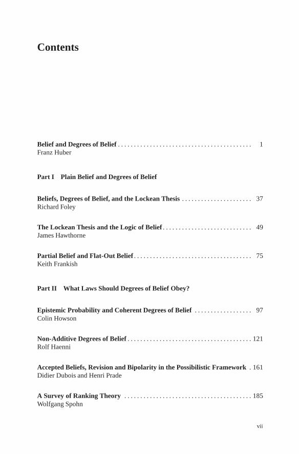
Contents

Belief and Degrees of Belief . . . . . . . . . . . . . . . . . . . . . . . . . . . . . . . . . . . . . . . . . . 1Franz Huber

Part I Plain Belief and Degrees of Belief

Beliefs, Degrees of Belief, and the Lockean Thesis . . . . . . . . . . . . . . . . . . . . . . 37Richard Foley

The Lockean Thesis and the Logic of Belief . . . . . . . . . . . . . . . . . . . . . . . . . . . . 49James Hawthorne

Partial Belief and Flat-Out Belief . . . . . . . . . . . . . . . . . . . . . . . . . . . . . . . . . . . . . 75Keith Frankish

Part II What Laws Should Degrees of Belief Obey?

Epistemic Probability and Coherent Degrees of Belief . . . . . . . . . . . . . . . . . . 97Colin Howson

Non-Additive Degrees of Belief . . . . . . . . . . . . . . . . . . . . . . . . . . . . . . . . . . . . . . . 121Rolf Haenni

Accepted Beliefs, Revision and Bipolarity in the Possibilistic Framework . 161Didier Dubois and Henri Prade

A Survey of Ranking Theory . . . . . . . . . . . . . . . . . . . . . . . . . . . . . . . . . . . . . . . . 185Wolfgang Spohn

vii

viii Contents

Arguments For—Or Against—Probabilism? . . . . . . . . . . . . . . . . . . . . . . . . . . 229Alan Hajek

Diachronic Coherence and Radical Probabilism . . . . . . . . . . . . . . . . . . . . . . . 253Brian Skyrms

Accuracy and Coherence: Prospects for an Alethic Epistemology ofPartial Belief . . . . . . . . . . . . . . . . . . . . . . . . . . . . . . . . . . . . . . . . . . . . . . . . . . . . . . 263James M. Joyce

Part III Logical Approaches

Degrees All the Way Down: Beliefs, Non-Beliefs and Disbeliefs . . . . . . . . . . 301Hans Rott

Levels of Belief in Nonmonotonic Reasoning . . . . . . . . . . . . . . . . . . . . . . . . . . . 341David Makinson

Contributors

Didier Dubois IRIT, Universite Paul Sabatier, Toulouse, France, [email protected]

Richard Foley New York University, New York, NY 10003, USA,[email protected]

Keith Frankish Department of Philosophy, The Open University, Walton Hall,Milton Keynes, MK7 6AA, UK, [email protected]

Rolf Haenni Bern University of Applied Sciences, Engineering and InformationTechnology, Hoheweg 80, CH-2501, Biel; Institute of Computer Science andApplied Mathematics, University of Bern, Neubruckstrasse 10, CH–3012, Bern,Switzerland, [email protected], [email protected]

Alan Hajek Research School of Social Sciences, Australian National University,Canberra, ACT 0200, Australia, [email protected]

James Hawthorne Department of Philosophy, University of Oklahoma, NormanOklahoma, 73019 USA, [email protected]

Colin Howson Department of Philosophy, Logic and Scientific Method,London School of Economics and Political Science, London WC2A 2AE, UK,[email protected]

Franz Huber Formal Epistemology Research Group, Zukunftskolleg andDepartment of Philosophy, University of Konstanz, Germany,[email protected]

James M. Joyce Department of Philosophy, University of Michigan, Ann Arbor,MI 48109-1003, USA, [email protected]

David Makinson London School of Economics, London WC2A 2AE, UK,[email protected]

Henri Prade IRIT, Universite Paul Sabatier, Toulouse, France, [email protected]

Hans Rott Department of Philosophy, University of Regensburg, 93040Regensburg, Germany, [email protected]

ix

x Contributors

Brian Skyrms Department of Logic and Philosophy of Science, Universityof California, Irvine 3151 Social Science Plaza, Irvine, CA 92697-5100, USA,[email protected]

Wolfgang Spohn Department of Philosophy, University of Konstanz, 78457Konstanz, Germany, [email protected]

Non-Additive Degrees of Belief

Rolf Haenni

Abstract The variety of formal approaches to numerical degrees of belief is divisi-ble into two main categories. They differ in the question of whether degrees of beliefof complementary hypotheses should sum up to one or not. The principal goal ofthis paper is to defend the position of non-additive degrees of belief. Another goal isto give an overview of approaches, point out their similarities and differences, andmake a link to existing historical roots. Particular attention is given to the Dempster-Shafer theory of evidence and the related theory of probabilistic argumentation. Thispaper is thought to serve as an extensive source of information, links, and referencesto the area of non-additive degrees of belief.

1 Introduction

This paper starts from the position that belief is primarily quantitative and not cat-egorical, i.e. we generally assume the existence of various degrees of belief. Thiscorresponds to the observation that most human beings experience belief as a mat-ter of degree. We follow the usual convention that such degrees of belief are valuesin the [0,1]-interval, including the two extreme cases 0 for “no belief ” and 1 for“full belief ”.1 Any other value in the unit interval represents its own level of certi-tude, thus allowing the quantification of statements like “I strongly believe ...” or “Ican hardly believe ...”. In this sense, we make a strict distinction between belief and

Rolf HaenniBern University of Applied Sciences, Engineering and Information Technology, Hoheweg 80, CH–2501, Biel, e-mail: [email protected] of Bern, Institute of Computer Science and Applied Mathematics, Neubruckstrasse 10,CH–3012 Bern, Switzerland, e-mail: [email protected]

1 A few authors proposed other belief scales such as [−1,+1] or R+. One of the most prominentexample is Spohn’s ranking theory [112, 113], where so-called ranks in R+ ∪∞ are assessed toexpress different gradings of disbelief.

1

2 Rolf Haenni

faith, the latter always being absolute. This position is in perfect accordance withthe following definition of belief:

Belief =

“Assent to the truth of something offered for acceptance. It may or may not imply certitude[...]. Faith almost always implies certitude.” [1]

Degrees of belief depend at least on two factors, namely the epistemic state of theperson who holds the belief, and the proposition or statement under consideration.The belief holder will subsequently be called agent, and with epistemic state werefer to the evidence or information that is available to the agent at a particular pointin time. The idea that belief depends on the available evidence is also included inthe following definition:

Belief =

“Mental acceptance of a proposition, statement, or fact, as true, on the ground of [...]evidence.” [2]

In a formal setting, we will talk about the degree of belief BelA,t(h) ∈ [0,1] of anagent A at time t with respect to a hypothesis h. The hypothesis itself is assumed tobe a proposition in a formal language that is either true or false, but the actual truthvalue of h is usually unknown to A. With ¬h we denote the complementary hypoth-esis that is true whenever h is false, and BelA,t(¬h) represents the correspondingdegree of belief in ¬h. Sometimes it is convenient to call BelA,t(¬h) degree of dis-belief [113] or degree of doubt [97]. Shackle referred to it as the degree of potentialsurprise [94, 95, 96], and 1−BelA,t(¬h) is sometimes called degree of plausibility[97, 109] or degree of possibility [37, 40].

1.1 Properties of Degrees of Belief

In an epistemic theory of belief, rational agents are expected to hold degrees of be-lief according to certain fundamental rules or laws. It is not our goal here to imposea comprehensive and universally acceptable axiomatic framework for degrees of be-lief, but rather to point out some of the most essential properties that most peoplewould be willing to accept, at least as a good approximation of the true characteris-tics of degrees of belief.2

In this respect, the first thing we assume is that if two agents A1 and A2 possessexactly the same amount of relevant information at time t, then they should holdequal degrees of belief with respect to a common hypothesis h. In other words, weassume that degrees of belief depend exclusively on the current amount of availableinformation, that is on the agent’s epistemic state, but not on the agent’s mentalstate as a whole. With this we exclude subjective preferences or any other form ofbias. If we call the available information at time t knowledge base3 and use ∆ t or

2 Smets gives such an axiomatic justification for Dempster-Shafer belief functions in [107].3 Smets prefers to call it evidential corpus ECA

t [109].

Non-Additive Degrees of Belief 3

simply ∆ to represent it, we may thus prefer to denote degrees of belief by Bel∆(h)rather than BelA,t(h). Often, ∆ will be expressed by set of sentences in a formallanguage, e.g. by logical or probabilistic constraints, but we do not further specifythis at this point. If ∆ (or A and t) is unambiguously determined by the context, wemay abbreviate Bel∆(h) by Bel(h). The process of building up degrees of belief froma given knowledge base is called reasoning.

Two of the most generally accepted properties of degrees of belief are consistencyand non-monotonicity. Consistency means that if a hypothesis h (logically) entailsanother hypothesis h′, then Bel(h) is expected to be smaller or equal than Bel(h′).We may thus impose that h |= h′ should imply Bel(h) ≤ Bel(h′), where |= meanslogical entailment. Additionally, we may assume that Bel(⊥) = 0 and Bel(>) = 1,where ⊥ denotes the hypothesis that is always false (and thus entails any otherpossible hypothesis) and > the hypothesis that is always true (and thus is entailedby any other possible hypothesis), respectively.

The non-monotonicity property tells us that obtaining new confirming (discon-firming) evidence may raise (lower) an agent’s degrees of belief.4 In general, learn-ing new information ∆′ (another set of logical or probabilistic constraints) will thusforce the agent to adapt existing degrees of belief non-monotonically in any possi-ble direction, depending on whether the new evidence supports or refutes currentdegrees of belief (or to leave them unchanged if ∆′ is already included in ∆ or if ∆′

is irrelevant to h):

Bel∆(h) S Bel∆∪∆′(h). (1)

More controversial is the question whether degrees of belief should be additiveor not. In this paper, we will assume non-additivity (or sub-additivity), which statesthat degrees of belief of complementary hypotheses h and ¬h do not necessarily addup to 1,

Bel(h)+Bel(¬h)≤ 1, (2)

or more generally, that the degrees of belief of two exclusive hypotheses h1 and h2do not necessarily add up to the degree of belief of their disjunction h1∨h2,

Bel(h1)+Bel(h2)≤ Bel(h1∨h2). (3)

Non-additivity is a direct consequence of assuming Bel /0(h) = 0 for all hypothesish 6=>. The idea of this is that the extreme case of total ignorance, expressed by anempty set ∆ = /0 of logical and probabilistic constraints, should never lead to degreesof belief different from zero (except for Bel /0(>) = 1). This reflects a very cautiousand sceptical attitude, according to which nothing is believed in the absence of sup-

4 In the context of inductive logic [27, 29, 45, 67], some authors start from the (stronger) criterion ofadequacy, which expects degrees of belief to converge towards 0 and 1, respectively: “As evidenceaccumulates, the degree to which the collection of true evidence statements comes to support ahypothesis, as measured by the logic, should tend to indicate that false hypotheses are probablyfalse and that true hypotheses are probably true” [47].

4 Rolf Haenni

porting evidence. This attitude implies Bel /0(h)+ Bel /0(¬h) = 0 for all h 66∈ ⊥,>,which is a particular case of the non-additivity assumption Bel(h)+ Bel(¬h) ≤ 1.Non-additive degrees of belief are appealing, since they allow a proper distinctionbetween uncertainty and ignorance (see Subsection 2.5). A number a different the-ories of uncertain reasoning are motivated by this, and it is what this paper is about.

Figure 1 illustrates how non-monotone and non-additive degrees of belief mayevolve if the available evidence ∆ t monotonically accumulates over time from aninitially empty set, i.e. if ∆ t ⊆ ∆ t ′ holds for all t ≤ t ′ and for ∆0 = /0.

Bel!t(h)

Bel!t(¬h)

t

0

1

0

Fig. 1 Non-monotone and non-additive degrees of belief.

Non-additive approaches to degrees of belief are in opposition to the Bayesianparadigm, according to which an agent’s degrees of belief are understood as subjec-tive probabilities and therefore follow the laws of probability theory [11, 85]. Updat-ing degrees of belief in the presence of new evidence (often called observations) isthen based on a rule that follows from Bayes’ theorem. Although the theorem itselfis undisputed, its usefulness depends on the ability to assign suitable prior proba-bilities. In the extreme case of no relevant background knowledge, e.g. for ∆ = /0, itmeans that an additive pair of values must be assigned to Bel /0(h) and Bel /0(¬h). Tosolve this problem, Bayesians tend to apply the principle of indifference (also calledthe principle of insufficient reason) [56], which states that if exclusive possibilitiesare indistinguishable (except for their names), then they are equally probable. Thisraises various problems such as various Bertrand-style paradoxes [22, 115]. In ourconcrete case of ∆ = /0, it implies Bel /0(h) = Bel /0(¬h) = 1/2 for all possible hypothe-ses h /∈ ⊥,>. The same conclusion results from applying the maximum entropyprinciple [79], a cautious version of the principle of insufficient reason, which in-structs us to choose the model with the greatest entropy [118].

From the perspective of a non-additive belief measure, additivity appears as anideal case in which degrees of belief coincide with long-run frequencies or sub-jective probabilities. There are numerous practical examples where the availableevidence is such that this ideal case actually occurs (for certain hypotheses), butthis seems not to be the case in general. As an example, consider the event of toss-ing a coin. In the ideal case, e.g. if the coin is known to be fair, one can concludefrom the available information ∆ = “the coin is fair” that the two possible out-


comes head and tail are equally (or at least nearly equally) probable. This impliesadditive degrees of belief Bel∆(head) = Bel∆(tail) = 1/2. However, if we supposethat nothing is known about the coin and the way it is tossed, we have a situationthat is quite different from the above ideal case, and non-additive degrees of beliefBel /0(head) = Bel /0(tail) = 0 seem to be more appropriate, particularly because theymake the obvious epistemic difference to the ideal case explicit. Dempster defendsthis point in one of his original papers:

“While it may count as a debit item that inferences are less precise than one might havehoped, it is a credit item that greater flexibility is allowed in the representation of a state ofknowledge.” [13, §1]

To strengthen the above argument about the coin tossing example, suppose thatthe coin toss is repeated, say 10 times, and that the outcome is 10 times head (seeLindley’s comment in the appendix of [13]). With a fair coin, we would certainlybe perplexed by the result, but most probably ascribe it to chance and continueto ascribe a degree of belief of 1/2 to future events head. With an unknown coin,however, we would regard the outcomes of the first 10 coin tosses as good evidencethat the coin is actually biased towards head and thus change our degree of beliefto a value closer to 1. Similar arguments in favor of non-additive degrees of belief,or in other words for adding a third category “don’t know” to the usual Bayesiandichotomy “h is true” or “h is false”, are given in [14, §2.4].

Another important argument for non-additive degrees of belief is the observa-tion that non-additivity is an implicit property of most formal logics. Since logic isusually not concerned with numbers, this is not very apparent at first sight. But ifwe consider logical entailment |= between a set of premises ∆ and a conclusion h,we may often encounter the case in which ∆ is insufficient to entail either h or itsnegation ¬h, i.e. where ∆ 6|= h and ∆ 6|= ¬h, and this translates most naturally intothe above-mentioned special case of total ignorance with Bel(h) = Bel(¬h) = 0.

1.2 Opinions

Beliefs in general and degrees of belief in particular are undoubtedly closely con-nected to an agent’s opinions. With the goal of representing different belief states,the term opinion has been introduced by Jøsang as the fundamental concept of whathe calls subjective logic [50, 51, 52, 53]. Essentially the same concept has beenstudied before under different names, first by Ginsberg [26] and later by Hajek et al.[43, 44] and Daniel [10]. In all cases, the starting point is a non-additive measure ofbelief, respectively a pair (b,d) of reals with b,d ≥ 0 and a+b ≤ 1. Here we focuson Jøsang’s original definition in [50], according to which an opinion with respectto a hypothesis h is a triple,5

5 Later in [51], opinions are defined as quadruples (b,d, i,a) with an additional component a, theso-called relative atomicity (we do not need this in this paper).

6 Rolf Haenni

ωh = (b,d, i), (4)

where b = Bel(h) is the degree of belief of the hypothesis h, d = Bel(¬h) the degreeof disbelief of h, and i = 1− (b+d) the so-called degree of ignorance.6 Since b, d,and i sum up to one by definition, opinions should be regarded as a two-dimensionalrather than three-dimensional concept, even if it is useful to always indicate all threedimensions for an improved readability. As shown in Figure 2, the set of all possibleopinions can be represented by a 2-simplex called opinion triangle [50]. To rep-resent a ternary probabilistic space, Dempster used a similar picture almost thirtyyears earlier in his most influential papers [12, 13]. Dempster did not have a par-ticular name, so he referred to it as barycentric coordinates, which is the correctmathematical term [9]. An isosceles triangle instead of a equilateral triangle wasused in [43] to picture the space of all degree of belief/disbelief pairs.

(0, 0, 1)

(1, 0, 0)(0, 1, 0)

Ignora

nce

BeliefDisb

elief

indi

!ere

nt

positivenegative

purelypositivepu

rely

nega

tive

Bayesian

neutral

extremalpositive

extremalnegative

Fig. 2 The opinion triangle with its three di-mensions.

Fig. 3 Special types of opinions.

To further illustrate the concept of an opinion with an example, suppose you meetan old friend from school after a long time. You remember her as a slim person,and except for her current balloon-shaped belly, this is still the case. Now consideryour updated opinion with regard to the the following three hypotheses: h1 =“Sheis pregnant”, h2 =“She is in the first month of pregnancy”, h3 =“This is her firstpregnancy”. Without any further information about your friend, your opinion ωh1will probably be close or equal to (1,0,0), ωh2 will be close or equal to (0,1,0), andωh3 will be close or equal to (0,0,1).

The three opinions in the above example are very particular extreme cases. Weadopt the terminology of [44], i.e. (1,0,0) and (0,1,0) are called extremal and(0,0,1) is called neutral.7 Examples of general opinions will be given in Subsec-tion 2.3 (see Example 2 and Figure 10). A general opinion ω = (b,d, i) is called

6 In [51], Jøsang calls i degree of uncertainty rather than degree of ignorance, but the latter seemsto be more appropriate and in better accordance with the literature (see Subsection 2.5).7 In the context of religious belief, they correspond to the positions of believers, atheists, andagnostics, respectively.


positive if b > d, and it is called negative if b < d. Positive opinions are located inthe right half and negative opinion in the left half of the opinion triangle. For b 6= d,(b,d, i) and (d,b, i) are called opposite opinions, i.e. the opposite of a positive opin-ion is negative, and vice versa.

In the opinion triangle, the two regions of positive and negative opinions are sepa-rated by the central vertical line of indifferent opinions for which b = d holds. Notethat the neutral opinion (0,0,1) is also indifferent. Another particular indifferentopinion is the point ( 1

2 , 12 ,0) at the bottom of the triangle.

Opinions are called pure if either b = 0 or d = 0, i.e. (b,0,1−b) is a purely pos-itive and (0,d,1−d) a purely negative opinion.8 More specifically, (1,0,0) is theextremal positive and (0,1,0) the extremal negative opinion. Pure opinions are lo-cated on the left and the right edge of the triangle. Finally, opinions (b,1−b,0) withi = 0, which form the bottom line of the triangle, are called Bayesian (or probabilis-tic). Note that the extremal opinions (1,0,0) and (0,1,0) are also Bayesian, as wellas the particular indifferent opinion ( 1

2 , 12 ,0). All those particular types of opinions

are shown in Figure 3.Notice that the special case of Bayesian opinions, which is unambiguously char-

acterized by a single (additive) value b ∈ [0,1], does not allow the agent to have “noopinion” or to say “I don’t know”. This limited expressiveness is why we think thatassuming additive degrees of belief is too restrictive for a general model of degreesof belief.

1.3 Related Work

Opinions as discussed above are implicitly included in many another approaches. Asmentioned earlier, a two-dimensional view of opinions has been studied by Gins-berg, Hajek et al., and Daniel in a proper algebraic setting, where pairs (b,d) arecalled Dempster pairs or simply d-pairs [10, 26, 43, 44]. The set of all such (non-extremal) Dempster pairs, together with Dempster’s rule of combination, forms acommutative semigroup with numerous interesting mathematical properties, e.g.that (0,0) is the neutral element of the combination.

Such belief/disbelief pairs are also obtained from probabilistic argumentation[34, 37], where b and d are the respective probabilistic weights of uncertain logicalarguments supporting the hypothesis and counter-arguments rejecting the hypothe-sis, respectively (see Section 3 for further details). In this particular context, b andd are also called degree of support and degree of refutation, respectively. One canthink of them as respective probabilities that the given evidence logically entails hor ¬h. Pearl questioned the usefulness of such probabilities of provability:

“Why should we concern ourselves with the probability that the evidence implies h, ratherthan the probability that h is true, given the evidence?” [82]

8 In [43], pure opinions are called simple.

8 Rolf Haenni

Of course, we would prefer having the latter, i.e. the ideal situation mentionedin the previous subsection, but the imperfection and incompleteness of the availableinformation does not provide this in general.

The term probability of provability (or probability of necessity) has first beenused by Pearl [81] and later by Laskey et al. in [71] and Smets in [106]. Ruspiniproposes a similar viewpoint, but he prefers to talk about epistemic probabilitiesP(Kh) and P(K¬h) of the epistemic states Kh (h is known) and K¬h (¬h is known),respectively [88, 89]. In Section 3, we will discuss this position in further detail.

The Dempster-Shafer theory [13, 97], also known as the theory of belief functionsor the theory of evidence, also yields such a pair of values, but the degree of disbe-lief Bel(¬h) is usually replaced by the degree of plausibility Pl(h) = 1−Bel(¬h).9

This implies 0 ≤ Bel(h) ≤ Pl(h) ≤ 1 for all possible hypotheses h and defines thusa partitioning of the unit interval [0,1] into three partitions. The same type of be-lief/plausibility pairs are used in Smets’ Transferable Belief Model (TBM) [109] andKohlas’ Theory of Hints [62]. Notice that the spirit behind such belief/plausibilitypairs is very similar to the modal operators (necessity) and ♦ (possibility) inmodal logic [7]. The connection to the opinion triangle is illustrated in Figure 4.

Bel(h) Pl(h)0 1

b di

!h

i

!h

0 1BetP (h)

Fig. 4 Belief and plausibility induced by anopinion ωh.

Fig. 5 Betting probability induced by anopinion ωh.

To obtain another two-dimensional representation of opinions, we may use theprinciple of indifference to transform Dempster pairs (b,d) into additive probabil-ities. In the TBM framework, this transformation is called pignistic transformation[109], and its result is called betting probability BetP(h). In the simple case of twocomplementary hypotheses h and ¬h, BetP(h) is simply the average over Bel(h) andBel(¬h). BetP(h) together with the degree of ignorance i = 1−Bel(h)−Bel(¬h) isanother possible two-dimensional view. It reflects the standpoint of some moderateBayesians, who admit that in addition to the (additive) degree of belief one should

9 The terms belief and plausibility were introduced by Shafer [97] as a replacement for whatDempster originally called lower and upper probability [12]. Note that Dempster’s lower and upperprobabilities are not to be confounded with lower and upper bounds obtained from inference withprobability intervals [68] or more generally with convex sets of probabilities [116].


also consider the strength of the belief, which depends on the amount of availablesupporting evidence. Hawthorne’s comment about this point goes as follows:

“I contend that Bayesians need two distinct notions of probability. We need the usual degree-of-belief notion that is central to the Bayesian account of rational decision. But Bayesiansalso need a separate notion of probability that represents the degree to which evidencesupports hypotheses.” [46, §1]

In this sense, additional supporting evidence can function in two ways: increasethe degree of belief or the strength of belief (or both). This point is the centralidea of what Schum [93] calls the Scandinavian School of Evidentiary Value [19,24], another non-additive approach to degrees of belief that is known today as theEvidentiary Value Model (EVM) [90]. It originates from the work of the Swedishlawyer Ekelof in the early sixties [20].

Instead of considering non-additive degrees of belief in the above sense, someauthors suggested so-called non-additive probabilities [25, 91, 92]. They are oftenunderstood as (lower and upper) bounds of probability intervals, which are inducedby sets of compatible probability functions [66, 68, 110, 117]. Today, the commongeneral term for this particular class of approaches is imprecise probabilities [116].Note that imprecise or non-additive probabilities have been in use in physics fora long time, where the role of the non-additivity is to describe the deviation ofelementary particles in mechanical wave-like behavior [23]. In this paper, in order toavoid unnecessary confusion, we prefer to make a strict distinction between additiveprobabilities (in the classical sense) and non-additive degrees of belief. In Section 3,we will see how to use the former to obtain the latter.

1.4 Historical Roots

As Shafer and later Kohlas pointed out [59, 98, 100, 101], examples of the two-dimensional (non-additive) view of degrees of belief can also be found in the lit-erature of the late seventeenth and early eighteenth centuries, well before Bayesianideas were developed. Historically, non-additive degrees of belief were mostly mo-tivated by judicial applications, such as the reliability of witnesses in the courtroom,or more generally by the credibility of testimonies on past events or miracles.

The first two combination rules for testimonies were published in 1699 in ananonymous article [3].10 One of those rules considers two witnesses with respec-tive credibilities (frequencies of saying the truth) p and p′. If we suppose that theydeliver the same report, they are either both telling the truth with probability pp′

or they are both lying with probability (1− p)(1− p′). Every other configuration

10 There is some disagreement about the authorship of this article. Shafer names the English clericGeorge Hooper (1640–1727) [99], but for Pearson, the true author is the English statistician Ed-mund Halley (1656–1742) [83]. Another possible author is the Scottish mathematician John Craig(1663–1731).

10 Rolf Haenni

is obviously impossible. The original formulation of the main statement goes asfollows:11

“The ratio of truth saying cases to the total number of cases,

pp′

pp′+(1− p)(1− p′), (5)

will represent the probability of both testifiers asserting the truth.” [3]

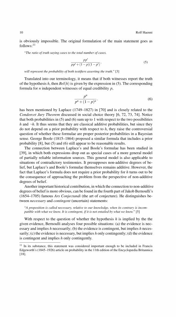
Translated into our terminology, it means that if both witnesses report the truthof the hypothesis h, then Bel(h) is given by the expression in (5). The correspondingformula for n independent witnesses of equal credibility p,

pn

pn +(1− p)n . (6)

has been mentioned by Laplace (1749–1827) in [70] and is closely related to theCondorcet Jury Theorem discussed in social choice theory [6, 72, 73, 74]. Noticethat both probabilities in (5) and (6) sum up to 1 with respect to the two possibilitiesh and ¬h. It thus seems that they are classical additive probabilities, but since theydo not depend on a prior probability with respect to h, they raise the controversialquestion of whether these formulae are proper posterior probabilities in a Bayesiansense. George Boole (1815–1864) proposed a similar formula that includes a priorprobability [8], but (5) and (6) still appear to be reasonable results.

The connection between Laplace’s and Boole’s formulae has been studied in[39], in which both expressions drop out as special cases of a more general modelof partially reliable information sources. This general model is also applicable tosituations of contradictory testimonies. It presupposes non-additive degrees of be-lief, but Laplace’s and Boole’s formulae themselves remains additive. However, thefact that Laplace’s formula does not require a prior probability for h turns out to bethe consequence of approaching the problem from the perspective of non-additivedegrees of belief.

Another important historical contribution, in which the connection to non-additivedegrees of belief is more obvious, can be found in the fourth part of Jakob Bernoulli’s(1654–1705) famous Ars Conjectandi (the art of conjecture). He distinguishes be-tween necessary and contingent (uncertain) statements:

“A proposition is called necessary, relative to our knowledge, when its contrary is incom-patible with what we know. It is contingent, if it is not entailed by what we know.” [5]

With respect to the question of whether the hypothesis h is implied by the thegiven evidence, Bernoulli analyses four possible situations: (a) the evidence is nec-essary and implies h necessarily; (b) the evidence is contingent, but implies h neces-sarily; (c) the evidence is necessary, but implies h only contingently; (d) the evidenceis contingent and implies h only contingently.

11 In its substance, this statement was considered important enough to be included in FrancisEdgeworth’s (1845–1926) article on probability in the 11th edition of the Encyclopædia Britannica[18].


In (c) and (d), a further distinction is made between pure and mixed arguments.In the mixed case, it is assumed that if the evidence does not imply h, it implies¬h, whereas nothing is said about ¬h in the pure case. Bernoulli then considers thenumber of cases in which the evidence occurs and in which h (or ¬h) is entailed.Finally, the corresponding ratios with respect to the total number of cases turn outto be non-additive in (b) and in the pure versions of (c) and (d).

Bernoulli also discusses the problem of combining several testimonies. Essen-tially, his combination rules are special cases of what is known today as Dempster’srule of combination (see Subsection 2.4 for details). In the mixed version of (c), theresults of the combination coincide with Laplace’s formula, again without requiringa prior probability for h. Laplace’s analysis is thus included in Bernoulli’s analysis,but the connection to non-additive degrees of belief is now more obvious.

Even more general is Johann Heinrich Lambert’s (1728–1777) discussion in[69]. From Lambert’s perspective, Bernoulli’s pure and mixed arguments are spe-cial cases of a more general situation, in which a syllogism (logical argument) hasthree parts, the affirmative, the negative, and the indeterminate. There is a numberattached to each of these parts, all three of them summing up to 1. This is exactlywhat is called today a Dempster pair (b,d) or an opinion ωh = (b,d, i). In this sense,Bernoulli’s distinction between pure and mixed arguments is a restriction to posi-tive and Bayesian opinions, respectively, but Lambert’s discussion covers the gen-eral case. A more comprehensive summary of Bernoulli’s, Lambert’s, and Laplace’swork with corresponding links to the modern view is given in [59, 98]. Notice thatthese very old ideas, until they were rediscovered by Dempster, Hacking, and Shaferat the end of the 20th century [12, 28, 97], were completely eliminated from main-stream probability over almost three full centuries.

2 Dempster-Shafer Theory

Probably the most influential and prominent non-additive approach to degrees ofbelief is the so-called Dempster-Shafer Theory (DST). It is designed to deal withthe distinction between uncertainty and ignorance. Rather than computing the prob-ability of an event H given some evidence, as in classical probability theory, thegoal here is to compute the probability that H is a necessity in the light of the avail-able evidence. This measure is called belief function Bel∆(H), and it satisfies all theproperties laid out in Subsection 1.1. Due to the central role of belief functions, DSTis sometimes called Theory of Belief Functions.

DST supposes the available information to be given in various pieces. We canthus think of ∆ = φ1, . . . ,φm as a collection of pieces or bodies of evidence φi.Smets calls such a set evidential corpus [109], but here we prefer the term knowledgebase, as suggested in Subsection 1.1. Each φ ∈ ∆ is encoded by a belief functionBelφ or the corresponding mass function mφ (see Subsection 2.2). If two or severalpieces of evidence are independent, then DST suggests a rule to combine them (seeSubsection 2.4). Formally, the result of the combination is denoted by φ1 ⊗φ2 (for

12 Rolf Haenni

a pair φ1 and φ2) and ⊗∆ (for the whole set ∆). The idea of combining evidence isfundamental in DST, and it includes Bayesian conditioning (derive posterior fromprior probabilities) as a special case.

The roots of DST go back to the late 1960s and Dempster’s concepts of lowerand upper probabilities, which result from a multi-valued mapping between twosample spaces Ω and Θ [12, 13]. The first space Ω carries an ordinary probabilitymeasure P, but the events of interests are subsets of Θ. In such a setting, we canuse the multi-valued mapping to turn the given probabilities given for Ω into lowerand upper probabilities for events H ⊆ Θ. In the early seventies, Glenn Shafer pro-posed a re-interpretation of Dempster’s lower probabilities as epistemic probabili-ties or degrees of belief. Shafer called his theory Mathematical Theory of Evidence[97], a name that is still in use. He took the rule for combining degrees of belief asfundamental. Since Shafer’s conjunctive combination rule was already included inDempster’s papers, he and most subsequent authors referred to it as Dempster’s ruleof combination (DRC). Nevertheless, Shafer’s original book is still one of the mostcomprehensive sources of information on DST.

In the late 1970s and early 1980s, Jeffrey Barnett brought Shafer’s theory into theAI community [4] and called it Dempster-Shafer theory (DST). Since then, numer-ous discussions, elaborations, and applications of DST were published by variousauthors. Particularly important contributions are Smets’ Transferable Belief Model[109] and Kohlas’ Mathematical Theory of Hints [62]. The more recent theory ofProbabilistic Argumentation proposes a new perspective, in which DST turns out tobe a unified theory of logical and probabilistic reasoning [34, 37, 40, 42, 60]. Thisapproach and its connection to DST will be discussed in Section 3.

In the late 1970s, the success story of DST was abruptly slowed down bya paper of Lotfi Zadeh, who presented an example for which Dempster’s ruleof combination produces results usually judged unsatisfactory or counter-intuitive[121, 122, 123, 124]. A common explanation is that possible conflicts between dif-ferent pieces of evidence are mismanaged by DRC. Since then, many authors haveused Zadeh’s example either to criticize DST as a whole, or as a motivation for con-structing alternative combination rules, which mainly differ from the way possibleconflicts are managed (the appendix of [108] gives a comprehensive overview ofsuch methods). Others do not reject DRC, but they try to fix the problem by consid-ering non-exclusive or non-exhaustive frames of discernment, see e.g. [104, 105]. Acritical note on the increasing number of possible combination rules and alternativeinterpretations of DST appeared in [30]. The most detailed and clarifying analysisof Zadeh’s puzzling example is given in [33]. Its conclusion is that it is not an in-trinsic problem of DRC, but a problem of its misapplication. We will briefly discussZadeh’s example in Subsection 2.4.

The goal of this section is to provide a rough overview of the main concepts,mathematical foundations, and different interpretations of DST. The discussion willbe restricted to finite frames, and only little or nothing will be said about computa-tion, implementation, or applications. For more information about these advancedtopics we refer to the corresponding literature, especially to the papers recently re-published as a collected volume [120].


2.1 Frame of Discernment

Belief is always related to a certain open question X . In general, we must considermany different possible answers for X . In the context of DST, it is assumed thatthere is a unique true (but unknown) answer. Such a question is therefore formallydescribed by a set ΘX of pairwise exclusive answers. Without loss of generality, wecan also assume ΘX to be exhaustive, i.e. the true answer is supposed to be one of itselements.12 Such an exhaustive and exclusive set ΘX is called frame of discernmentor simply frame [97]. Some authors call it universe of discourse or simply universe.In a context, in which X is unambiguously determined, we may simply write Θ

instead of ΘX . In the following, we make the additional assumption that Θ is finite.In the context of DST and with respect to a given frame ΘX , a hypothesis or

event is a subset H ⊆ ΘX of values.13 H is true if it contains the true answer of X ,otherwise it is false. 2Θ denotes the set of all subsets (power set) of Θ, i.e. the set ofall possible hypotheses.

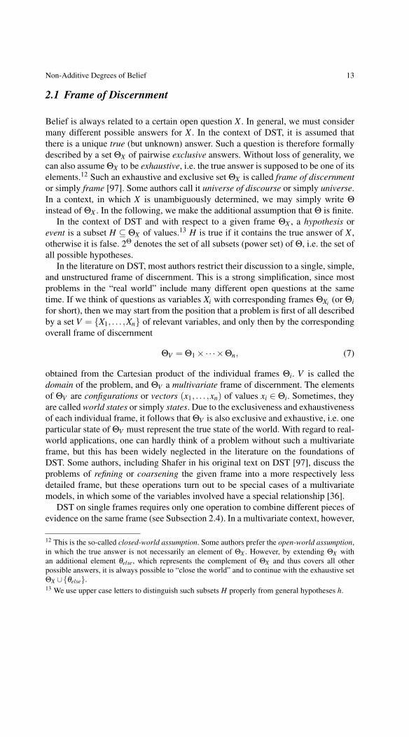
In the literature on DST, most authors restrict their discussion to a single, simple,and unstructured frame of discernment. This is a strong simplification, since mostproblems in the “real world” include many different open questions at the sametime. If we think of questions as variables Xi with corresponding frames ΘXi (or Θifor short), then we may start from the position that a problem is first of all describedby a set V = X1, . . . ,Xn of relevant variables, and only then by the correspondingoverall frame of discernment

ΘV = Θ1×·· ·×Θn, (7)

obtained from the Cartesian product of the individual frames Θi. V is called thedomain of the problem, and ΘV a multivariate frame of discernment. The elementsof ΘV are configurations or vectors (x1, . . . ,xn) of values xi ∈ Θi. Sometimes, theyare called world states or simply states. Due to the exclusiveness and exhaustivenessof each individual frame, it follows that ΘV is also exclusive and exhaustive, i.e. oneparticular state of ΘV must represent the true state of the world. With regard to real-world applications, one can hardly think of a problem without such a multivariateframe, but this has been widely neglected in the literature on the foundations ofDST. Some authors, including Shafer in his original text on DST [97], discuss theproblems of refining or coarsening the given frame into a more respectively lessdetailed frame, but these operations turn out to be special cases of a multivariatemodels, in which some of the variables involved have a special relationship [36].

DST on single frames requires only one operation to combine different pieces ofevidence on the same frame (see Subsection 2.4). In a multivariate context, however,

12 This is the so-called closed-world assumption. Some authors prefer the open-world assumption,in which the true answer is not necessarily an element of ΘX . However, by extending ΘX withan additional element θelse, which represents the complement of ΘX and thus covers all otherpossible answers, it is always possible to “close the world” and to continue with the exhaustive setΘX ∪θelse.13 We use upper case letters to distinguish such subsets H properly from general hypotheses h.

14 Rolf Haenni

every piece of evidence may concern a different (sub-)set of variables, and combin-ing them is thus a bit more complicated. If φ denotes a single piece of evidence,then we write d(φ)⊆V for the corresponding domain (set of relevant variables) ofφ. Working with such general cases requires then two additional operations, one toextend φ to larger domains D ⊇ d(φ) and one to project or marginalize it to smallerdomains d ⊆ d(φ). The extension operator is useful to transform two pieces of evi-dence φ1 and φ2 to their common domain d(φ1)∪d(φ2), which allows then the useof the normal combination operator. Sometimes, this particular type of extension isconsidered to be part of the combination operator. Such an extended combinationtogether with the marginalization operator, which is needed to focus the given infor-mation to one or some of the variables involved (the questions of interest), forms thebasis of so-called valuation or information algebras [59, 102]. This is an axiomaticinformation theory for which general inference procedures exist [32, 63, 103].

In this section, we will not further discuss DST with multivariate frames orvaluation-based inference. But we want to emphasize that these topics are of crucialimportance, not only for successfully applying and implementing DST to real-worldproblems, but also for a deeper and more comprehensive understanding of this the-ory. An particular variant of DST, in which multivariate frames are fundamental,will be presented in Section 3.

2.2 Mass Functions

The Bayesian view of additive degrees of belief is mainly based on the idea thatan agent’s total belief is dispersible into various portions. Additionally, if the agentcommits a certain degree of belief to a proposition, the remainder must be commit-ted to its alternatives. These are the two main features of the Bayesian approach. Tomake it more general, the obvious thing to do is to keep the first of these featureswhile discarding the second. In other words, the additivity property is no longerimposed. This is the fundamental idea that finally leads to DST.

At the core of DST is thus the idea that any piece of evidence φ, for a given frameof discernment Θ, is encoded by a function

mφ : 2Θ → [0,1], (8)

which maps every subset A ⊆ Θ of possible answers into a number mφ(A) of the[0,1]-interval, with the condition that

∑A⊆Θ

mφ(A) = 1. (9)

In a context in which the evidence φ is unambiguously clear, mφ is often ab-breviated by m. In Shafer’s book, such m-functions are called basic probability as-signments (bpa), and a single value mφ(A) is a basic probability number [97]. Thecommon names today are mass function for m and belief mass or simply mass of


A for single values m(A).14 A mass function m is called normalized, if additionallym( /0) = 0 holds, otherwise it is called unnormalized. Some authors prefer to restricttheir discussion to normalized mass functions, because no belief mass ought to becommitted to the empty set. This follows from the exhaustiveness of Θ. However,it is mathematically more convenient to allow unnormalized mass functions and totake care of the exhaustiveness later. In such an unnormalized context, m( /0) is calledconflicting mass.

A set A ⊆ Θ with mφ(A) > 0 is called focal set or focal element of φ. The set ofall focal elements is denoted by Fφ, and its union Cφ =

⋃Fφ is the core of φ. Mass

functions with respect to a frame Θ are similar to discrete probability distributions(also called probability mass functions), except that the values are assigned to sub-sets A ⊆ Θ instead of singletons θ ∈ Θ. Discrete probability distributions are thusspecial cases of mass functions, namely if all focal elements are singletons. Suchmass functions are called Bayesian or precise.

There is a number of other particular classes of mass functions. Vacuous massfunctions represent the case of total ignorance and are characterized by m(Θ) = 1(and thus m(A) = 0 for all strict subsets A⊂Θ). Simple mass functions have at mostone focal element distinct from Θ. Deterministic mass functions have exactly onefocal element. Consonant mass functions have nested focal elements, i.e. it is pos-sible to number the r elements Ai ∈ Fφ such that A1 ⊂ ·· · ⊂ Ar. The characteristicsof these classes are depicted in Figure 6.

! ! ! !!

a) Bayesian b) Vacuous c) Simple d) Deterministic e) Consonant

Fig. 6 Different classes of mass functions.

Each of these classes has its own special mathematical properties. The combi-nation of two Bayesian mass functions, for example, yields another Bayesian massfunction. For more details on this we refer to the literature [62, 97].

In Shafer’s original view, a belief mass m(A) should be understood as “[...] themeasure of belief that is committed exactly to A, [...]not the total belief one commitsto A” [97]. This is one possible interpretation, in which mass functions (or belieffunctions) are considered to be the “atoms” with which evidence is described. Thisis also the view defended in Smets’ Transferable Belief Model [109] and in Jøsang’sSubjective Logic [50], and it is the view that dominates the literature on DST today.

14 Smets prefers to talk about basic belief assignments (bba) for m-functions m and basic beliefmasses for single values m(A) [109].

16 Rolf Haenni

A similar viewpoint is the one in which belief masses are regarded as random sets[75, 76].

A slightly different perspective is offered by Dempster’s original concept ofmulti-valued mappings [12], where mass functions indirectly arise from two samplespaces Ω and Θ, a mapping

Γ : Ω → 2Θ (10)

from Ω to the power set of Θ, and a corresponding (additive) probability measure Pover Ω. Formally, the connection from such a multi-valued mapping to mass func-tions is given by

m(A) = ∑ω∈Ω,

Γ(ω)=A

P(ω) (11)

This is also Kohlas’s view in his Theory of Hints [62], where a quadrupleφ = (Ω,P,Γ,Θ) is called hint, and the elements ω of the additional set Ω are under-stood as possible interpretations of the hint.15 Probability remains thus the essentialconcept for both Dempster and Kohlas, whereas mass functions or non-additive de-grees of belief are induced as secondary elements. This is also the starting point inthe area of probabilistic argumentation [34], which will be discussed in Section 3.Shafer supports Dempster’s probabilistic view with the following words:

“The theory of belief functions is more flexible; it allows us to derive degrees of belief for aquestion from probabilities for a related question. These degrees of belief may or may nothave the mathematical properties of probabilities; how much they differ from probabilitieswill depend on how closely the two questions are related.” [99]

In the common foreword of [120], a recently published collected volume on clas-sic works of the Dempster-Shafer theory, both Dempster and Shafer strengthen thispoint:

“Some authors [...] have tried to distance the Dempster-Shafer theory from the notion ofprobability. But we have long believed that the theory is best regarded as a way of usingprobability. Understanding of this point is blocked by superficial but well entrenched dog-mas that still need to be overcome.”

From a mathematical point of view, one can always construct a multi-valuedmapping (or a hint) for a given mass function, such that (11) holds. On the otherhand, (11) can always be used to reduce a multi-valued mapping into a mass func-tion. Deciding between the two possible interpretations of DST is thus like trying tosolve the chicken and egg problem. However, Dempster’s probabilistic view offersat least the following three advantages:

• The first advantage is the fact that nothing more than the basic laws of probabilityand set theory is required. This is certainly less controversial than any attempt toaxiomatize DST in terms of belief or mass functions (an example of such anattempt is given in [107]).

15 In [43], a hint (Ω,P,Γ,Θ) is called Dempster space or simply d-space.


• The second advantage comes from the observation that transforming a multi-valued mapping or hint into a mass function always implies some loss of in-formation. If Θ is the only question of interest, this loss may be of little or noimportance, but this is not always the case.

• The third advantage is connected to the combination rule (see Subsection 2.4),for which Dempster’s probabilistic view offers a clear and unambiguous under-standing, in particular with respect to what is meant with independent pieces ofevidence.

The fact that the independence requirement has become one of the most con-troversial points of DST is presumably a consequence of today’s dominating non-probabilistic view and its attempt to see combination as a self-contained rule that isentirely detached from the notion of probabilistic independence.

Example 1. To illustrate the difference between the two possible views, consider theexample of a murder case in court, where some irrevocable evidence allows us to re-duce the list of suspects to an exhaustive and exclusive set Θ = John,Peter,Mary.Let W be a witness testifying that Peter was at home at crime time, and suppose thecourt judges W ’s reliability with a subjective (additive) probability of 0.8. Noticethat W ’s statement is not necessarily false if W is unreliable. We may thus denoteW ’s testimony by φW and represent it with an additional set ΩW = relW ,¬relW,the probabilities PW (relW) = 0.8 and PW (¬relW) = 0.2, and the multi-valuedmapping

ΓW (relW ) = John,Mary,ΓW (¬relW ) = John,Peter,Mary,

from ΩW to Θ. Altogether we obtain a hint φW = (ΩW ,PW ,ΓW ,Θ). The correspond-ing (simple) mass function mW over Θ, which we obtain with the aid of (11), hasthus two focal elements John,Mary and John,Peter,Mary, and it is defined by

mW (John,Mary) = 0.8,

mW (John,Peter,Mary) = 0.2.

Notice that the hint φW describes the given evidence with respect to two distinctquestions, whereas mW affects Θ only. The complete hint is thus more informativethan the mass function mW alone. The representations are illustrated in the picturesshown in Figure 7 and Figure 8.

To avoid the loss of information, we may start with a multivariate frame Θ′ =ΩW ×Θ from the beginning. The resulting mass function m′

W has again two focalsets and is similar to mW from above, but now all the information with respect toboth variables Ω and Θ is included:

m′W ((relW ,John),(relW ,Mary)) = 0.8,

m′W ((¬relW ,John),(¬relW ,Peter),(¬relW ,Mary)) = 0.2.

18 Rolf Haenni

Peter

John

Mary

!

0.8

0.2

!W

¬relW

relW

Peter

John

Mary

!

0.8

0.2

Fig. 7 The complete multi-valued mappingof the murder case example.

Fig. 8 The evidence reduced to a mass func-tion.

After all, the choice between a multi-valued mapping from Ω to Θ or a massfunction over the complete frame Ω×Θ turns out to be a matter of taste, whereasreducing the evidence to Θ alone means to lose information.

2.3 Belief and Plausibility Functions

Following Shafer’s original view, according to which “the quantity m(A) measuresthe belief that one commits exactly to A” [97], we obtain the total degree of beliefcommitted to a hypothesis H ⊆Θ by summing up the masses m(A) of all non-emptysubsets A⊆H. In the general case, where m is not necessarily normalized, it is addi-tionally necessary to divide this sum by 1−m( /0). This is a necessary consequenceof the exhaustiveness of Θ. Belief functions are finally defined as follows:

Bel(H) =1

1−m( /0) ∑/06=A⊆H

m(A). (12)

One can easily show that this definition is in accordance with all the basic prop-erties for degrees of belief laid out in Subsection 1.1, including non-additivity. Inthe case of a normalized mass function, it is possible to simplify (12) into

Bel(H) = ∑A⊆H

m(A). (13)

This is the definition commonly found in the literature. An alternative definitionis obtained from Dempster’s perspective of a multi-valued mapping. It is evidentthat the elements of the so-called support set SH = ω ∈ Ω : Γ(ω) ⊆ H are thestates in which H is a necessary consequence of the given evidence. In other words,every element ω ∈ SH supports H, and

P(SH) = ∑ω∈SH

P(ω) (14)


denotes the corresponding prior probability that H is supported by the evidence.In the general (unnormalized) case, we must additionally consider the conflict setS /0 = ω ∈ Ω : Γ(ω) = /0 of impossible states, the ones that are incompatible withthe exhaustiveness assumption. P(SH) must thus be conditioned on the complementof S /0. Note that S /0 ⊆ SH holds for all possible H ⊆ Θ. This leads to the followingalternative definition of belief functions:

Bel(H) = P(SH |Sc/0) =

P(SH ∩Sc/0)

P(Sc/0)

=P(SH\S /0)1−P(S /0)

=P(SH)−P(S /0)

1−P(S /0). (15)

It is easy to verify that (15) together with (11) and (14) leads to (12). The twodefinitions are thus mathematically equivalent. But (15) has the advantage of pro-viding a very clear and transparent semantics, in which Bel(H) is the probability ofprovability or probability of necessity of H in the light of the given model [81, 106].We will give a similar definition in the context of probabilistic argumentation (seeSection 3), where the same measure is called degree of support.

Due to the non-additive nature of belief functions, Bel(H) alone is not enough todescribe an agent’s full opinion with regard to a hypothesis H. Shafer calls Bel(Hc)degree of doubt and 1−Bel(Hc) upper probability of H [97]. The latter expressesthe extent to which H appears credible or plausible in the light of the evidence.Today, it is more common to talk about the plausibility

Pl(H) = 1−Bel(Hc) (16)

of H. This definition implies 0 ≤ Bel(H) ≤ Pl(H) ≤ 1 for all H ⊆ Θ. Note thatcorresponding mass, belief, and plausibility functions convey precisely the same in-formation. A given piece of evidence φ is thus fully and unambiguously representedby either function mφ, Belφ, or Plφ. Another possible representation is the so-calledcommonality function qφ [97], which possesses some interesting mathematical prop-erties. We refer to the literature for more information on commonality functions andon how to transform one representation into another.

Example 2. To further illustrate the connection between mass, belief, and plausi-bility functions, let’s look at another numerical example. Consider a frame Θ =A,B,C,D and an unnormalized mass function m with four non-zero values m( /0) =0.2, m(C) = 0.1, m(A,B) = 0.4, and m(B,C) = 0.3. The focal sets are thus/0, C, A,B, and B,C. Table 1 shows for all possible hypotheses H ⊆ Θ thevalues Bel(H) and Pl(H) as obtained from (12) and (16).

H /0 A B C A,B A,C B,C A,B,C

m(H) 0.2 0 0 0.1 0.4 0 0.3 0

Bel(H) 0 0 0 0.125 0.5 0.125 0.5 1

Pl(H) 0 0.5 0.875 0.5 0.875 1 1 1

Table 1 The connection between mass, belief, and plausibility functions.

20 Rolf Haenni

!

A

B

C

0.4

0.3

0.1

!1

!2

!3

!4

0.2 !!

!A,B,C

!A,B

!A,C

!B,C

!C

!B

!A

!!

Fig. 9 The complete multi-valued mapping. Fig. 10 The opinions for all H ⊆ Θ.

In the case of H = B,C, for example, we have two relevant focal sets, namelyC and B,C. If we divide the sum m(C)+m(B,C) = 0.1+0.3 = 0.4 of theirmasses by 1−m( /0) = 1−0.2 = 0.8, we obtain Bel(B,C) = 0.4/0.8 = 0.5. Thisand the fact that A is the complement of B,C implies Pl(A) = 1−0.5 = 0.5.

If we start, as indicated in Figure 9, from a hint φ = (Ω,P,Γ,Θ) with two setsΩ = ω1,ω2,ω3,ω4 and Θ = A,B,C,D, a multi-valued mapping Γ(ω1) = /0,Γ(ω2) = C, Γ(ω3) = A,B, Γ(ω4) = B,C, and corresponding probabilitiesP(ω1) = 0.2, P(ω2) = 0.1, P(ω3) = 0.4, P(ω4) = 0.3, we can derive thesame values from the support sets with the aid of (15) and (16). Table 2 lists thenecessary details for all H ⊆ Θ.

H /0 A B C A,B A,C B,C A,B,C

SH ω1 ω1 ω1 ω1,ω2 ω1,ω3 ω1,ω2 ω1,ω2,ω4 ω1,ω2,ω3,ω4SH\S /0 ω2 ω3 ω2 ω2,ω4 ω2,ω3,ω4

P(SH\S /0) 0 0 0 0.1 0.4 0.1 0.4 0.8

Bel(H) 0 0 0 0.125 0.5 0.125 0.5 1

Pl(H) 0 0.5 0.875 0.5 0.875 1 1 1

Table 2 Belief and plausibility functions induced by a hint.

Each pair of values Bel(H) and Pl(H) leads to an opinion in the sense of the def-inition given in Subsection 1.2. The opinions for all hypotheses H ⊆Θ are depictedin Figure 10. Note that the opinions of complementary hypotheses are symmetricwith respect to the vertical center line.

2.4 Dempster’s Rule of Combination

Representing evidence by mass, belief, or plausibility functions is the first key con-cept of DST. The second one is a general rule for combining such mass, belief, or


plausibility functions when they are based on independent pieces of evidence. In itsgeneral form, this combination rule was first described in Dempster’s original articlein which DST was founded [12]. Dempster called it orthogonal sum, but today mostauthors refer to it as Dempster’s rule of combination (DRC). Formally, the combina-tion of two pieces of evidence φ1 and φ2 is denoted by φ1⊗φ2. Some authors preferto write m1⊗m2 or Bel1⊗Bel2 for the combination of corresponding mass or belieffunctions, but here we will write mφ1⊗φ2

and Belφ1⊗φ2, respectively.

The most accessible and intuitive description of DRC is obtained in terms ofmass functions. In the following, let mφ1

and mφ2be two mass functions represent-

ing independent pieces of evidence φ1 and φ2 on the same frame of discernment Θ

(the problem of combining mass functions on distinct frames and the related topicof multivariate frames has been discussed in Subsection 2.1). Recall that we do notrequire the mass functions to be normalized, which allows us to define the unnor-malized version of DRC as follows:

mφ1⊗φ2(A) = ∑

A1∩A2=Amφ1

(A1)mφ2(A2). (17)

Note that (17) may produce a conflicting mass different from 0 even if both mφ1and mφ2

are normalized. In the normalized version of DST, which is slightly morecommon in the literature, it is therefore necessary to divide the right-hand expressionof (17) by the so-called (re-)normalization constant

k = 1− ∑A1∩A2= /0

mφ1(A1)mφ2

(A2), (18)

which corresponds to the division by 1−m( /0) in (12). In the following, we will usethe unnormalized rule together with (12). In either case, we may restrict the sets A1and A2 in (17) to the focal elements of m1 and m2. This is important for an efficientimplementation of DRC.

Dempster’s rule has a number of interesting mathematical properties. The mostimportant ones are commutativity, i.e. φ1 ⊗ φ2 = φ2 ⊗ φ1, and associativity, i.e.φ1 ⊗ (φ2 ⊗ φ3) = (φ1 ⊗ φ2)⊗ φ3. The order in which evidence is combined is thusirrelevant. This allows us to write ⊗∆ = φ1⊗·· ·⊗φm for the combined evidenceobtained from a set ∆ = φ1, . . . ,φm. DRC also satisfies all other properties of avaluation algebra [59], i.e. the general inference mechanisms for valuation algebrasare also applicable to DST.

An important prerequisite for DRC is the above-mentioned independence as-sumption. But what exactly does it mean for two mass or belief functions to beindependent? This question is one of the most controversial issues related to DST.However, if we start from two hints φ1 = Ω1,Θ,Γ1,P1 and φ2 = Ω2,Θ,Γ2,P2instead of two mass functions m1 and m2, it is possible to define independence withrespect to pieces of evidence in terms of standard probabilistic independence be-tween Ω1 and Ω2, for which marginal probabilities P1 respectively P2 are given.The joint probability over the Cartesian product Ω12 = Ω1×Ω2 is then the prod-

22 Rolf Haenni

uct P12 = P1P2, i.e. P12(ω) = P1(ω1)P2(ω2) is the probability of an elementω = (ω1,ω2) ∈ Ω12 in the product space.

If we suppose that ω = (ω1,ω2) ∈ Ω12 is the true state of Ω12, then φ1 impliesthat the true state of Θ is in Γ1(ω1), whereas φ2 implies that the true state of Θ

is in Γ2(ω2). As a consequence, we can conclude that the true state of Θ is inΓ1(ω1)∩Γ2(ω2). Combining two hints φ1 and φ2 thus means to pointwise multiplyprobabilities and intersect corresponding focal sets. This is the core of the followingalternative definition of Dempster’s rule:

φ12 = φ1⊗φ2 = (Ω12,P12,Γ12,Θ) = (Ω1×Ω2,P1P2,Γ1∩Γ2,Θ). (19)

If we use (11) to obtain the mass functions mφ1, mφ2

, and mφ12from φ1, φ2, and

φ12, respectively, it is easy to show that mφ1⊗mφ2

= mφ12holds. Mathematically,

the two definitions of DRC given in (17) and (19) are thus equivalent. But since (19)defines the underlying independence assumption unambiguously in terms of prob-abilistic independence, it offers a less controversial understanding of DRC. Unfor-tunately, this view is far less common in the literature than the one obtained from(17). An axiomatic justification of the latter is included in [105].

Example 3. Consider the murder case of Example 1 and suppose that a secondwitness V , who saw the crime from a distance, testifies with 90% certainty thatthe murderer is male, i.e. either John or Peter. Of course, if V is mistaken aboutthe gender, the murderer is Mary. In addition to the hint φW given in Exam-ple 1, we must now consider a second hint φV = (ΩV ,PV ,ΓV ,Θ with respect tothe same frame Θ = John,Peter,Mary, but with ΩV = relV ,¬relV, the multi-valued mapping ΓV (relV ) = John,Peter, ΓV (¬relV ) = Mary, and the probabil-ities PV (relV) = 0.9 and PV (¬relV) = 0.1. Combining the two hints accord-ing to (19) produces then a new hint φWV = φW ⊗ φV = (ΩWV ,PWV ,ΓWV ,Θ) withΩWV = relW relV ,relW¬relV ,¬relW relV ,¬relW¬relV, PWV = PW PV , and the fol-lowing multi-valued mapping:

ΓWV (relW relV ) = John, PWV (relW relV) = 0.72,

ΓWV (relW¬relV ) = Mary, PWV (relW¬relV) = 0.08,

ΓWV (¬relW relV ) = John,Peter, PWV (¬relW relV) = 0.18,

ΓWV (¬relW¬relV ) = Mary, PWV (¬relW¬relV) = 0.02.

If the resulting hint φWV is transformed into a mass function, we get mWV (John) =0.72, mWV (John,Peter) = 0.18, and mWV (Mary) = 0.08 + 0.02 = 0.1. It iseasy to verify that the same result is obtained from applying (17) to mW and mV .

Example 4. Let’s have short look at Zadeh’s example of disagreeing experts. In theliterature, the example appears in different but essentially equivalent versions. Onepossible version is the story of a doctor who reasons about possible diseases. LetΘ = M,C,T be the set of possible diseases (M stands for meningitis, C for con-cussion, and T for tumor), i.e. exactly one of these diseases is supposed to be the


true disease. In order to further restrict this set, suppose the doctor consults twoother experts E1 and E2 who give him the following reports:

E1: “I am 99% sure it’s meningitis, but there is a small chance of 1% that it’sconcussion.”

E2: “I am 99% sure it’s a tumor, but there is a small chance of 1% that it’s con-cussion.”

Encoding these statements according to Zadeh’s analysis leads to two mass func-tions m1 and m2 defined by

m1(A) =

0.99, for A = M0.01, for A = C0, for all other A ⊆ Θ

, m2(A) =

0.99, for A = T0.01, for A = C0, for all other A ⊆ Θ

.

Combining m1 and m2 with the aid of the unnormalized version of DRC leads thento a new mass function m defined by

m12(A) = m1⊗m2(A) =

0.0001, for A = C0.9999, for A = /00, for all other A ⊆ Θ

.

Note that m12 is highly conflicting. Normalization according to (12) then leads toBel12(M) = Bel12(T) = 0 and Bel12(C) = 1, from which the doctor con-cludes that C is the right answer, i.e. the patient suffers from concussion. In thelight of the given statements from E1 and E2, this conclusion seems to be counter-intuitive. How can a disease such as C, which has almost completely been ruled outby both experts, become the only remaining option?

Mathematically, the situation is very clear. The puzzling result is due to thefact that m1(T) = 0 completely eliminates T as a possible answer, whereasm2(M) = 0 entirely excludes M, thus leaving C as the only possible answer. Inother words, E1 implicitly says that T is wrong (with absolute certainty), and E2says that M is wrong (with absolute certainty). Together with the assumption that Θ

is exclusive and exhaustive, it follows then that C remains as the only possible trueanswer.16 The result obtained from Zadeh’s example is thus a simple logical con-sequence of the given information. This is the starting point of the analysis in [33],in which not Dempster’s rule but Zadeh’s particular way of modeling the availableevidence is identified to be the cause of the puzzle. In a more sophisticated model, inwhich (1) the possible diseases are not necessarily exclusive and/or (2) the experts

16 In Sir Arthur Conan Doyle’s The Sign of Four [16], Sherlock Holmes describes this type ofsituation as follows: “How often have I said to you that when you have eliminated the impossible,whatever remains, however improbable, must be the truth”. In A Study in Scarlet [17], he refers toit as the method of exclusion: “By the method of exclusion, I had arrived at this result, for no otherhypothesis would meet the facts”. For more information about Sherlock Holmes’s way of reasoningwe refer to [114].

24 Rolf Haenni

are not fully reliable, Dempster’s rule turns out to be in full accordance with whatintuitively would be expected. For more details we refer to the discussion in [33].

2.5 Aleatory vs. Epistemic Uncertainty

From the perspective of the hint model, i.e. with the multi-valued mapping from aprobability space Ω to another set Θ in mind, DST seems to make a distinction be-tween different types of uncertainty. The first one is represented with the aid of theprobability measure P over Ω, whereas the second one manifests itself in the multi-valued mapping Γ from Ω to Θ. Traditionally, probability theory has been used tocharacterize both types of uncertainty, but recently, the scientific and engineeringcommunity has begun to recognize the utility of defining multiple types of uncer-tainty. According to [48], the dual nature of uncertainty should be described withthe following definitions:

• Epistemic Uncertainty: The type of uncertainty which results from the lack ofknowledge about a system and is a property of the analysts performing the anal-ysis (also known as: subjective uncertainty, type B uncertainty, reducible un-certainty, state of knowledge uncertainty, model form uncertainty, ambiguity,ignorance).

• Aleatory Uncertainty: The type of uncertainty which results from the fact that asystem can behave in random ways (also known as: stochastic uncertainty, type Auncertainty, irreducible uncertainty, variability, objective uncertainty, randomuncertainty);

One of the most distinguishing characteristics between epistemic and aleatory un-certainty is the fact that the former is a property of the analyst or agent, whereasthe latter is tied to the system under consideration. As a consequence, it is pos-sible to reduce epistemic uncertainty with research, which is not the case foraleatory uncertainty. In realistic problems, aleatory and epistemic uncertainties aremostly intricately interwoven. Some authors prefer to simply distinguish betweenuncertainty (for aleatory uncertainty) and ignorance (for epistemic uncertainty)[31, 54, 55, 111].

It is well recognized that aleatory uncertainty is best dealt with the frequentistapproach associated with classical probability theory, but fully capturing epistemicuncertainty seems to be beyond the capabilities of traditional additive probabilities.This is where the benefits of non-additive approaches such as DST start. WithinDST, for example, it is possible to represent the extreme case of full aleatory uncer-tainty (e.g. tossing a fair coin) by a uniform probability distribution over Ω, whereasfull epistemic uncertainty (e.g. tossing an unknown coin) is modeled by Γ(ω) = Θ

for all ω ∈ Ω. DST allows thus a proper distinction between both types of uncer-tainty, which is not the case with standard (first-order) probabilities alone.17 With

17 Some probabilists try to evade the problem of properly distinguishing between epistemicand aleatory uncertainty using second-order probability distributions over first-order probabilities


respect to a hypothesis H, this distinction finally leads to a two-dimensional quanti-tative result Bel(H)≤ Pl(H) and thus to a general opinion in the sense of the discus-sion in Subsection 1.2. The i-value of such an opinion is a measure of the epistemicuncertainty, including the extreme cases of i = 0 (no epistemic uncertainty) and i = 1(total epistemic uncertainty).

What are the benefits of distinguishing two types of uncertainty? First, by takinginto account the possibility of lacking knowledge or missing data, we get a morerealistic and more complete picture with regard to the hypothesis to be evaluated inthe light of the given knowledge. Second, if reasoning serves as a preliminary stepfor decision making, a proper measure of ignorance is useful to decide whether theavailable knowledge justifies an immediate decision. The idea is that high degreesof ignorance imply low confidence in the results. On the other hand, low degrees ofignorance result from situations where the available knowledge forms a solid basisfor a decision. Therefore, decision making should always consider the additionaloption of postponing the decision until enough information is available.18 The studyof decision theories with the option of further deliberation is a current research topicin philosophy of economics [15, 55, 92]. Apart from that, decision making underignorance is a relatively unexplored discipline. For an overview of attempts in thecontext of Dempster-Shafer theory we refer to [77].

3 Probabilistic Argumentation

As we have seen, the capability of DST to represent both types of epistemic andaleatory uncertainty is a result of the multi-valued mapping from a probability spaceΩ into another set Θ. Now suppose that both Ω and Θ are complex sets, e.g. productspaces relative to some underlying variables. This is the typical situation in mostreal-world applications. Note that Ω may be a sub-space of Θ.

The problem of working with such complex sets is to specify the multi-valuedmapping. The explicit enumeration of all (ω,Γ(ω))-pairs is certainly not practical.The idea now, which leads us to the topic of this section, is to use a logical languageLV over a set V of variables. The simplest case of such a language is the language ofpropositional logic, where V degenerates into a set of propositional variables [40].Other typical languages are obtained from finite set constraints [41], interval con-straints [78], or general multivariate constraints such as (linear) equations and/or

[68, 80]. The shape (or the variance) of the underlying density function allows then the discrim-ination of different situations, e.g. a flat shape for full epistemic uncertainty or one peaking at1/2 for full aleatory uncertainty. In addition to the increased mathematical complexity, various ob-jections have been raised against second-order probabilities. One important point is the apparentnon-applicability of “Dutch book” arguments [111].18 It’s like in real life: people do not like decisions under ignorance. In other words, people preferbetting on events they know about. This psychological phenomenon is called ambiguity aversionand has been experimentally demonstrated by Ellsberg [21]. His observations are rephrased inEllsberg’s paradox, which is often used as an argument against decision-making on the basis ofsubjective probabilities.

26 Rolf Haenni

inequalities [61, 119]. The goal thus is to exploit the expressive power and flexibil-ity of such languages in the context of DST.

The basic requirement is that the language defines a proper logical consequenceoperator on the basis of a multi-dimensional state space. Together with the prob-ability measure defined over Ω, we obtain then a unified theory of probabilis-tic and logical reasoning, which is known in the literature as the theory of prob-abilistic argumentation [34, 37, 60]. This theory demonstrates how to decoratethe mathematical foundations of DST with the expressiveness and convenienceof a logical language. As an extract of [34] and [37], this section gives a shortintroduction. We refer to the literature for examples of successful applications[35, 38, 39, 49, 57, 58, 64, 65, 84, 86, 87].

3.1 Unifying Logic and Probability

Logic and probability theory have both a long history in science. They are mainlyrooted in philosophy and mathematics, but are nowadays important tools in manyother fields such as computer science and, in particular, artificial intelligence. Somephilosophers studied the connection between logical and probabilistic reasoning,and some attempts to combine these disciplines have been made in computer sci-ence, but logic and probability theory are still widely considered to be separatetheories that are only loosely connected.

In order to build such a unifying theory, we must first try to better understand theorigin of the differences between logical and probabilistic reasoning. In this respect,one of the key points to realize is based on the following simple observation: pureprobabilistic reasoning usually presupposes the existence of a probability measureover all variables in the model, whereas logical reasoning does not deal with prob-abilities at all, i.e. it presupposes a probability function over none of the variablesinvolved. If we call the variables over which a probability function is known proba-bilistic, we can say that a probabilistic model consist of probabilistic variables only,whereas all variables of a logical model are non-probabilistic. From this point ofview, the main difference between logical and probabilistic reasoning is the num-ber of probabilistic variables. This simple observation turns out to be crucial forunderstanding some of the main similarities and differences between logical andprobabilistic reasoning.19

With this remark in mind, building a more general theory of reasoning is quitestraightforward. The simple idea is to allow an arbitrary number of probabilisticvariables. More formally, if V is the set of all variables involved in the model, wesuppose to have a subset W ⊆ V of probabilistic variables. If ΩX denotes the finiteset of possible values (or states) of a single variable X ∈V and ΩS = ΩX1 ×·· ·×ΩXs

the corresponding Cartesian product for a subset S = X1, . . . ,Xs⊆V , then we con-

19 The literature on how to combine logic and probability is huge, but the idea of distinguishingprobabilistic and non-probabilistic variables seems to be relatively new.


sider a probability measure P : 2ΩW → [0,1] w.r.t. the σ -algebra of subsets of ΩW .20

Clearly, logical reasoning is characterized by W = /0 and probabilistic reasoningby W = V , but we are now interested in the more general case of arbitrary sets ofprobabilistic variables. This is the conceptual starting point of the theory of proba-bilistic argumentation. The connection between probabilistic argumentation and theclassical fields of logical and probabilistic reasoning is illustrated in Figure 11.

0% 100%

ProbabilisticReasoning

LogicalReasoning

ProbabilisticArgumentation

Percentage ofProbabilisticVariables

Fig. 11 Different sets of probabilistic variables.

In addition to the probability measure over ΩW , let the given knowledge orevidence be encoded by a set Φ ⊆ LV of logical sentences. It determines a setEV = JΦK ⊆ ΩV of admissible states, the models of Φ, and it is assumed that thetrue state of the world is exactly one element of EV . A probabilistic argumentationsystem is then defined as a quintuple

A = (V,LV ,Φ,W,P). (20)

This is the mathematical structure into which the available evidence is compiled.We will see later that every probabilistic argumentation systems defines a hint witha corresponding multi-valued mapping from ΩW to ΩV .

Example 5. Alice flips a fair coin and promises to invite us to a barbecue tomorrownight provided that the coin lands on head. Alice is well-known to always keep herpromises, but she does not say anything about what she is doing in case the coinlands on tail, i.e. she may or may not organize the barbecue in that case. Of course,we would like to know whether the barbecue takes place or not. How can this storybe expressed in terms of a probabilistic argumentation system?

The given evidence consists of two pieces: the first one is Alice’s reliablepromise, and the second one is the fact that the two possible outcomes of toss-ing a fair coin are known to be equally likely. Thus the evidence is best mod-eled with two Boolean variables, say H (for head) and B (for barbecue), with do-

20 Note that the finiteness assumption with regard to ΩW is not a conceptual restriction of thistheory, but it allows us to define P with respect to the σ -algebra 2ΩW and thus helps to keep themathematics simple.

28 Rolf Haenni

mains ΩH = ΩB = 0,1, a (uniform) probability function over ΩH , and a proposi-tional sentence h → b (with h and b as placeholders for the atomic events H = 1and B = 1, respectively). We have thus V = H,B, Φ = h → b, W = H,and P(h) = P(¬h) = 0.5. Altogether we get a probabilistic argumentation systemA = (V,LV ,Φ,W,P) as defined above, where LV is the language of propositionallogic over V .

3.2 Degree of Support

With respect to a given probabilistic argumentation system A = (V,LV ,Φ,W,P),the problem to solve is to evaluate quantitatively whether a hypothesis, expressed asa sentence h ∈ LV , is true or false. Let H = JhK ⊆ ΩV be the corresponding set ofmodels of h, i.e. h is true if and only if the true state of the world is an element of H.In the general case, i.e. for Φ 66|= h and Φ 6|= ¬h, the question is how to use the givenprobability measure P for judging the possible truth of h.

For judging a hypothesis h ∈ LV , the key concept is the notion of degree ofsupport, denoted by dsp(h) ∈ [0,1]. The formal definition given below is based ontwo observations. The first one is the fact that the set EV ⊆ ΩV , which restricts theset of possible states relative to V , also restricts the possible states relative to W . Theelements s ∈ ΩW are called scenarios, and P(s) denotes the corresponding priorprobability of s. By projecting EV from ΩV onto ΩW , we get the set EW = E↓W

V ⊆ΩWof scenarios that are consistent with EV . This means that exactly one element of EWcorresponds to the true state of the world in ΩV , and all other scenarios s ∈ΩW\EWare impossible. This tells us to condition P on EW , i.e. to replace the given priorprobability P(·) by a posterior probability P′(·) = P(·|EW ). EW thus plays the roleof the evidence, which is used to update P in a Bayesian way. This mechanism isillustrated in Figure 12 for the particular case of V = X ,Y and W = X.

The second observation goes in the other direction, that is from ΩW to ΩV . Let’sassume that a certain scenario s ∈ ΩW is the true scenario. This reduces the set ofpossible states with respect to V from EV to

EV |s = x ∈ EV : x↓W = s, (21)

where x↓W denotes the projection of the state x from V to W . Thus, EV |s contains allatomic events of EV that are compatible with s. This idea is illustrated in Figure 13for V = X ,Y, W = X, and four scenarios s0, s1, s2, and s3. Note that s ∈ EWimplies EV |s 6= /0 and vice versa. Consider then a consistent scenario s ∈ EW forwhich EV |s ⊆ H holds. In logical terms, this means that Φ|s |= h holds, where Φ|sdenotes the set of logical sentences obtained from Φ by instantiating all probabilisticvariables according to s. Since h is a logical consequence of s and Φ, and we can sees as a defeasible or hypothetical proof for h in the light of Φ. We must say defeasible,because it is generally unknown whether s is the true scenario or not. In other words,h is only supported by s, but not entirely proven. Such supporting scenarios are also


!X

!Y

EV

EW

P !(·) = P (·|EW ) P (·)

!X

!Y

EV H

s0 s1 s2

EV |s2

EV |s1

s3

EV |s3

Fig. 12 Prior and posterior distributions overprobabilistic variables.

Fig. 13 Evidence conditioned on variousscenarios.

called arguments for h, and the set of all arguments for h is denoted by

ARGS(h) = s ∈ EW : Φ|s |= h= s ∈ ΩW : ⊥ 6≡ Φ|s |= h. (22)

The elements of the set ARGS(¬h) are sometimes called counter-arguments ofh. In other words, they refute h in the light of the given evidence. In the example ofFigure 8, the hypothesis h is supported by s3, but not by s0, s1, or s2 (s0 is inconsis-tent). Similarly, ¬h is supported (or h is refuted) by s1, but not by s0, s1, or s3. Inthe case of s2, nothing definite is known about h. The existence of such neutral sce-narios is the reason why degrees of support (see definition below) are non-additive.The decomposition of the set ΩW into supporting, refuting, neutral, and inconsistentscenarios is depicted in Figure 14.

!W

EW

!W \EW

ARGS (h)

ARGS (¬h)

!|s |= h

!|s |= ¬h

!|s !|= ¬h

!|s !|= h

!|s |= !

Fig. 14 Supporting, refuting, neutral, and inconsistent scenarios.

30 Rolf Haenni

The above definition of supporting arguments is the key notion for the follow-ing definition of degree of support. In fact, because every arguments s ∈ ARGS(h)contributes to the possible truth of h, we can measure the strength of such a contri-bution by the posterior probability P′(s) = P(s|EW ), and the total support for hcorresponds to the sum

dsp(h) = ∑s∈ARGS(h)

P′(s) = P′(ARGS(h)) =P(ARGS(h))

P(EW )(23)

over all elements of ARGS(h). The fact that the sets ARGS(h) and ARGS(¬h) are notnecessarily complementary (or exhaustive) implies dsp(h)+ dsp(¬h) ≤ 1. Degreesof support should therefore be understood as non-additive posterior probabilities ofprovability. Under the condition that Φ 6|= ⊥, they are well-defined for all possiblehypotheses h ∈ LV , that is even in cases in which the prior probability P does notcover all variables. This is the main advantage over classical probabilistic reasoning,which presupposes the existence of a prior distribution over all variables. For moretechnical details on probabilistic argumentation we refer to [37].

3.3 Connection to Dempster-Shafer Theory

The connection between probabilistic argumentation and DST is quite straightfor-ward, especially if by looking at DST from the hint perspective and a correspondingmulti-valued mapping between two spaces. If we start from a probabilistic argumen-tation system (V,LV ,Φ,W,P), we simply need to set Γ(s) = EV |s for all s ∈ ΩWto obtain a corresponding hint (ΩW ,P,Γ,ΩV ). To see that the two definitions ofBel(H) and dsp(h) coincide, consider the definition of the support set SH in Sub-section 2.3. In the current context, we get SH = s ∈ ΩW : EV |s ⊆ H and thereforeS /0 = s∈ΩW : EV |s = /0. This implies EW = ΩW \S /0, which allows us to transformthe third expression of (15) into (23):

Bel(H) =P(SH ∩EW )

P(EW )=

P(s ∈ EW : EV |s ⊆ H)P(EW )

=P(ARGS(h))

P(EW )= dsp(h).

This shows that DST and probabilistic argumentation are mathematically equiva-lent. Another way to show this equivalence is to transform all sentences φ ∈ Φ intocorresponding mass functions mφ, and to combine them with the Bayesian massfunction mP derived from P, This transformation is also interesting from a com-putational point of view, but for further details we refer to [42]. Finally, it is alsopossible to express any arbitrary mass function as a probabilistic argumentation sys-tem and formulate Dempster’s combination rule as a particular form of merging twoprobabilistic argumentation systems.

Despite these technical similarities, the theories are still quite different from aconceptual point of view. Dempster’s rule of combination, for example, which is


one of the central concepts in the Dempster-Shafer theory, is no big issue in thetheory of probabilistic argumentation. Another difference is the fact that the notionsof belief and plausibility in the Dempster-Shafer theory are often entirely detachedfrom a probabilistic interpretation (especially in Smets’s TBM framework), whereasdegrees of support are probabilities by definition. Finally, while the use of a logi-cal language to express factual information is an intrinsic part of a probabilisticargumentation system, it is an almost unknown technique in the Dempster-Shafertheory. In other words, probabilistic argumentation demonstrates how to decoratethe mathematical foundations of Dempster-Shafer theory with the expressivenessand convenience of a logical language.

3.4 Logical and Probabilistic Reasoning

To complete this section, let us briefly investigate how the classical fields of logicaland probabilistic reasoning fit into this general theory. As mentioned earlier, logicalreasoning is simply characterized by W = /0. This has a number of consequences.First, it implies that the set of possible scenarios ΩW = 〈〉 consists of a singleelement 〈〉, which represents the empty vector of values. This means that P(〈〉) =1 fully specifies the prior probability. Furthermore, we have EV |〈〉 = EV , whichallows us to simplify (22) into

ARGS(h) =

〈〉, for ⊥ 6≡ Φ|s |= h/0, otherwise.

(24)

Finally, if we assume Φ 6|= ⊥, we get EW = 〈〉 = ΩW and thus P′(〈〉) = 1,and this implies

dsp(h) =

1, for Φ |= h,

0, otherwise,(25)

which corresponds to the usual understanding of provability in the context of logicalreasoning.

Probabilistic reasoning, on the other hand, is characterized by W = V , whichagain has a number of consequences. Most obviously, we have ΩW = ΩV and thusE = EW = EV . This implies

E|s =

s, for s ∈ E,

/0, otherwise,(26)

from which we conclude that ARGS(h) = H ∩E and therefore

32 Rolf Haenni

dsp(h) =P(H ∩E)

P(E)= P(H|E), (27)

which is the usual way of defining posterior probabilities in the context of proba-bilistic reasoning.

Probabilistic argumentation is therefore a true generalization of the two classicaltypes of logical and probabilistic reasoning. This is a remarkable conclusion, whichlifts probabilistic argumentation from its original intention as a theory of argumen-tative reasoning up to a unified theory of logical and probabilistic reasoning.

4 Conclusion

Non-additive degrees of belief seem to arise naturally from the skeptical attitude ofnot believing anything without available supporting evidence. Accepting this posi-tion means to understand degrees of belief as epistemic degrees of supports ratherthan Bayesian probabilities. A direct consequence of this alternative view is theintuitive concept of an opinion, which allows all possible combined situations ofbelief, disbelief, and epistemic ignorance to be properly discriminated. This is thecommon conceptual starting point of numerous formal approaches to non-additivedegrees of belief, among which Dempster-Shafer theory is the most prominent one.Interestingly, the same ideas were already present in the 17th and 18 century, i.e. inthe early days of probability theory.

An alternative perspective is to see non-additive degrees of belief as the result ofcombining the basic characteristics of logical and probabilistic reasoning. This is themotivation of the theory of probabilistic argumentation, which shows how to enrichthe mathematical foundations of Dempster-Shafer theory with the expressivenessand convenience of a logical language. At the same time, a precise response is givento a very fundamental question in the are of reasoning and inference, namely howthe areas of logic and probability theory are connected.

Acknowledgements Thanks to Michael Wachter for helpful remarks and proof-reading. This re-search is supported by the Swiss National Science Foundation, Project No. PP002–102652.

References

1. Merriam-Webster Online Dictionary. URL http://www.m-w.com2. Oxford English Dictionary. URL http://dictionary.oed.com3. Anonymous Author: A calculation of the credibility of human testimony. Philosophical

Transactions of the Royal Society 21, 359–365 (1699)4. Barnett, J.A.: Computational methods for a mathematical theory of evidence. In: P.J. Hayes

(ed.) IJCAI’81, 7th International Joint Conference on Artificial Intelligence, pp. 868–875.Vancouver, Canada (1981)

5. Bernoulli, J.: Ars Conjectandi. Thurnisiorum, Basel (1713)


6. Black, D.: Theory of Committees and Elections. Cambridge University Press, Cambridge,USA (1958)

7. Blackburn, P., de Rijke, M., Venema, Y.: Modal Logic. Cambridge University Press (2001)8. Boole, G.: The Laws of Thought. Walton and Maberley, London (1854)9. Bottema, O.: On the area of a triangle in barycentric coordinates. Crux Mathematicorum 8,

228–231 (1982)10. Daniel, M.: Algebraic structures related to Dempster-Shafer theory. In: B. Bouchon-Meunier,

R.R. Yager, L.A. Zadeh (eds.) IPMU’94, 5th International Conference on Information Pro-cessing and Management of Uncertainty in Knowledge-Based Systems, LNCS 945, pp. 51–61. Springer, Paris, France (1994)

11. de Finetti, B.: La prevision: ses lois logiques, ses sources subjectives. Annales de l’InstitutHenri Poincare 7(1), 1–68 (1937)

12. Dempster, A.P.: Upper and lower probabilities induced by a multivalued mapping. Annals ofMathematical Statistics 38, 325–339 (1967)

13. Dempster, A.P.: A generalization of Bayesian inference. Journal of the Royal StatisticalSociety 30(2), 205–247 (1968)

14. Dempster, A.P.: The Dempster-Shafer calculus for statisticians. International Journal of Ap-proximate Reasoning 48(2), 365–377 (2008)

15. Douven, I.: Decision theory and the rationality of further deliberation. Economics and Phi-losophy 18(2), 303–328 (2002)

16. Doyle, A.C.: The sign of four. Lippincott’s Magazine (1890)17. Doyle, A.C.: A study in scarlet, pt. 2. Beeton’s Christmas Annual (1890)18. Edgeworth, F.Y.: Probability. In: H. Chisholm (ed.) Encyclopædia Britannica, vol. 22, 11th

edn., pp. 376–403. University of Cambridge (1911)19. Edman, M.: Adding independent pieces of evidence. In: Modality, Morality and other

Problems of Sense and Nonsense: Essays dedicated to Soren Hallden, pp. 180–191. CWKGleerups, Lund, Sweden (1973)

20. Ekelof, P.O.: Rattegang, 6th edn. Norstedts Juridik AB, Stockholm, Sweden (1992)21. Ellsberg, D.: Risk, ambiguity, and the Savage axioms. Quarterly Journal of Economics 75,

643–669 (1961)22. Erickson, G.W.: Dictionary of Paradox. University Press of America (1998)23. Feynman, R.P., Leighton, R.B., Sands, M.: The Feynman Lectures on Physics, vol. I, 2nd

edn. Addison-Wesley (1963)24. Gardenfors, P., Hansson, B., Sahlin, N.E. (eds.): Evidentiary Value: Philosophical, Judicial

and Psychological Aspects of a Theory. CWK Gleerups, Lund, Sweden (1983)25. Gilboa, I.: Expected utility with purely subjective non-additive probabilities. Journal of

Mathematical Economics 16, 65–88 (1987)26. Ginsberg, M.: Non-monotonic reasoning using Dempster’s rule. In: R.J. Brachman (ed.)

AAAI’84, 4th National Conference on Artificial Intelligence, pp. 112–119. Austin, USA(1984)

27. Gustason, W.: Reasoning from Evidence: Inductive Logic. Prentice Hall (1998)28. Hacking, I.: The Emergence of Probability. Cambridge University Press (1975)29. Hacking, I.: An Introduction to Probability and Inductive Logic. Cambridge University Press

(2001)30. Haenni, R.: Are alternatives to Dempster’s rule alternatives? – Comments on “About the

belief function combination and the conflict management problem”. International Journal ofInformation Fusion 3(3), 237–241 (2002)

31. Haenni, R.: Ignoring ignorance is ignorant. Tech. rep., Center for Junior Research Fellows,University of Konstanz, Germany (2003)

32. Haenni, R.: Ordered valuation algebras: a generic framework for approximating inference.International Journal of Approximate Reasoning 37(1), 1–41 (2004)

33. Haenni, R.: Shedding new light on Zadeh’s criticism of Dempster’s rule of combination.In: FUSION’05, 8th International Conference on Information Fusion, vol. 2, pp. 879–884.Philadelphia, USA (2005)

34 Rolf Haenni

34. Haenni, R.: Towards a unifying theory of logical and probabilistic reasoning. In: F.B. Coz-man, R. Nau, T. Seidenfeld (eds.) ISIPTA’05, 4th International Symposium on ImpreciseProbabilities and Their Applications, pp. 193–202. Pittsburgh, USA (2005)

35. Haenni, R.: Using probabilistic argumentation for key validation in public-key cryptography.International Journal of Approximate Reasoning 38(3), 355–376 (2005)

36. Haenni, R.: Uncover Dempster’s rule where it is hidden. In: FUSION’06, 9th InternationalConference on Information Fusion, contribution No. 251. Florence, Italy (2006)

37. Haenni, R.: Probabilistic argumentation. Journal of Applied Logic (2008)38. Haenni, R., Hartmann, S.: A general model for partially reliable information sources. In:

P. Svensson, J. Schubert (eds.) FUSION’04, 7th International Conference on InformationFusion, vol. I, pp. 153–160. Stockholm, Sweden (2004)

39. Haenni, R., Hartmann, S.: Modeling partially reliable information sources: a general ap-proach based on Dempster-Shafer theory. International Journal of Information Fusion 7(4),361–379 (2006)

40. Haenni, R., Kohlas, J., Lehmann, N.: Probabilistic argumentation systems. In: D.M. Gabbay,P. Smets (eds.) Handbook of Defeasible Reasoning and Uncertainty Management Systems,vol. 5: Algorithms for Uncertainty and Defeasible Reasoning, pp. 221–288. Kluwer Aca-demic Publishers, Dordrecht, Netherlands (2000)

41. Haenni, R., Lehmann, N.: Building argumentation systems on set constraint logic. In:B. Bouchon-Meunier, R.R. Yager, L.A. Zadeh (eds.) Information, Uncertainty and Fusion,pp. 393–406. Kluwer Academic Publishers, Dordrecht, Netherlands (2000)

42. Haenni, R., Lehmann, N.: Probabilistic argumentation systems: a new perspective onDempster-Shafer theory. International Journal of Intelligent Systems, Special Issue on theDempster-Shafer Theory of Evidence 18(1), 93–106 (2003)

43. Hajek, P., Havranek, T., Jirousek, R.: Uncertain Information Processing in Expert Systems.CRC Press, Boca Raton, USA (1992)

44. Hajek, P., Valdes, J.J.: Generalized algebraic approach to uncertainty processing in rule-basedexpert systems (dempsteroids). Computers and Artificial Intelligence 10, 29–42 (1991)

45. Harrod, R.: Foundations of Inductive Logic. Macmillan (1974)46. Hawthorne, J.: Degree-of-belief and degree-of-support: Why Bayesians need both notions.

Mind 114(454), 277–320 (2005)47. Hawthorne, J.: Inductive logic. In: E.N. Zalta (ed.) The Stanford Encyclopedia of Philosophy.

Center for the Study of Language and Information, Stanford University, USA (2005). URLhttp://plato.stanford.edu/archives/sum2005/entries/logic-inductive/

48. Helton, J.C.: Uncertainty and sensitivity analysis in the presence of stochastic and subjectiveuncertainty. Journal of Statistical Computation and Simulation 57, 3–76 (1997)

49. Jonczy, J., Haenni, R.: Credential networks: a general model for distributed trust and authen-ticity management. In: A. Ghorbani, S. Marsh (eds.) PST’05, 3rd Annual Conference onPrivacy, Security and Trust, pp. 101–112. St. Andrews, Canada (2005)

50. Jøsang, A.: Artificial reasoning with subjective logic. In: A.C. Nayak, M. Pagnucco (eds.)2nd Australian Workshop on Commonsense Reasoning. Perth, Australia (1997)

51. Jøsang, A.: A logic for uncertain probabilities. International Journal of Uncertainty, Fuzzi-ness and Knowledge-Based Systems 9(3), 279–311 (2001)

52. Jøsang, A.: The consensus operator for combining beliefs. Artificial Intelligence 141(1),157–170 (2002)

53. Jøsang, A., Bondi, V.A.: Legal reasoning with subjective logic. Artificial Intelligence andLaw 8(4), 289–315 (2000)

54. Katzner, D.W.: Time, Ignorance, and Uncertainty in Economic Models. University of Michi-gan Press (1998)

55. Kelsey, D., Quiggin, J.: Theories of choice under ignorance and uncertainty. Journal ofEconomic Surveys 6(2), 133–53 (1992)

56. Keynes, J.M.: A Treatise of Probability. Macmillan, London (1921)57. Khosla, D.: Method and apparatus for joint kinematic and feature tracking us-

ing probabilistic argumentation. United States Patent No. 7026979 (2006). URLhttp://www.wikipatents.com/7026979.html


58. Khosla, D., Chen, Y.: Joint kinematic and feature tracking using probabilistic argumenta-tion. In: FUSION’03, 6th International Conference on Information Fusion, vol. I, pp. 11–16.Cairns, Australia (2003)

59. Kohlas, J.: Information Algebras: Generic Stuctures for Inference. Springer, London (2003)60. Kohlas, J.: Probabilistic argumentation systems: A new way to combine logic with probabil-

ity. Journal of Applied Logic 1(3–4), 225–253 (2003)61. Kohlas, J., Monney, P.A.: Propagating belief functions through constraint systems. Interna-

tional Journal of Approximate Reasoning 5, 433–461 (1991)62. Kohlas, J., Monney, P.A.: A Mathematical Theory of Hints – An Approach to the Dempster-

Shafer Theory of Evidence, Lecture Notes in Economics and Mathematical Systems, vol.425. Springer (1995)

63. Kohlas, J., Shenoy, P.P.: Computation in valuation algebras. In: D.M. Gabbay, P. Smets(eds.) Handbook of Defeasible Reasoning and Uncertainty Management Systems, vol. 5: Al-gorithms for Uncertainty and Defeasible Reasoning, pp. 5–39. Kluwer Academic Publishers,Dordrecht, Netherlands (2000)

64. Kohlas, R.: Decentralized trust evaluation and public-key authentication. Ph.D. thesis, Uni-versity of Bern, Switzerland (2007)

65. Kohlas, R., Jonczy, J., Haenni, R.: A trust evaluation method based on logic and probabilitytheory. In: IFIPTM’08, 2nd Joint iTrust and PST Conferences on Privacy Trust Managementand Security. Trondheim, Norway (2008)

66. Koopman, B.O.: The axioms and algebra of intuitive probability. Annals of Mathematics andArtificial Intelligence 41, 269–292 (1940)

67. Kyburg, H.E.: Probability and Inductive Logic. Macmillan, New York, USA (1970)68. Kyburg, H.E.: Higher order probabilities and intervals. International Journal of Approximate

Reasoning 2, 195–209 (1988)69. Lambert, J.H.: Neues Organon oder Gedanken uber die Erforschung und Bezeichnung des

Wahren und dessen Unterscheidung vom Irrtum und Schein. Johann Wendler, Leipzig (1764)70. Laplace, P.S.: Theorie Analytique des Probabilites, 3eme edn. Courcier, Paris (1820)71. Laskey, K.B., Lehner, P.E.: Assumptions, beliefs and probabilities. Artificial Intelligence

41(1), 65–77 (1989)72. List, C.: On the significance of the absolute margin. British Journal for the Philosophy of

Science 55(3), 521–544 (2004)73. List, C., Goodin, R.E.: Epistemic democracy: Generalizing the Condorcet jury theorem. Jour-

nal of Political Philosophy 9(3), 277–306 (2001)74. Marquis de Condorcet: Essai sur l’application de l’analyse a la probabilite des decisions

rendues a la pluralite des voix. L’Imprimerie Royale, Paris, France (1785)75. Matheron, G.: Random Sets and Integral Geometry. John Wiley and Sons (1975)76. Nguyen, H.T.: On random sets and belief functions. Journal of Mathematical Analysis and

Applications 63, 531–542 (1978)77. Nguyen, H.T., Walker, E.A.: On decision making using belief functions. In: R.R. Yager,

J. Kacprzyk, M. Fedrizzi (eds.) Advances in the Dempster-Shafer Theory of Evidence, pp.311–330. John Wiley and Sons, New York, USA (1994)

78. Older, W., Vellino, A.: Constraint arithmetic on real intervals. In: F. Benhamou, A. Colmer-auer (eds.) Constraint Logic Programming: Selected Research, pp. 175–196. MIT Press(1993)

79. Paris, J.: The Uncertain Reasoner’s Companion – a Mathematical Perspective. No. 39 inCambridge Tracts in Theoretical Computer Science. Cambridge University Press (1994)

80. Pearl, J.: How to do with probabilities what people say you can’t. In: CAIA’85, 2nd IEEEConference on AI Applications, pp. 6–12. Miami, USA (1985)

81. Pearl, J.: Probabilistic Reasoning in Intelligent Systems. Morgan Kaufmann, San Mateo,USA (1988)

82. Pearl, J.: Reasoning with belief functions: An analysis of compatibility. International Journalof Approximate Reasoning 4(5–6), 363–389 (1990)

36 Rolf Haenni

83. Pearson, K.: The History of Statistics in the 17th and 18th Centuries against the Chang-ing Background of Intellectual, Scientific and Religious Thought: Lectures by Karl Pearsongiven at University College (London) during the Academic Sessions 1921–1933. Lubrecht& Cramer, London, U.K. (1978)

84. Picard, J., Savoy, J.: Using probabilistic argumentation systems to search and classify websites. IEEE Data Engineering Bulletin 24(3), 33–41 (2001)

85. Ramsey, F.P.: Truth and probability. In: R.B. Braithwaite (ed.) The Foundations of Mathe-matics and other Logical Essays, chap. 7, pp. 156–198. Routledge, London, U.K. (1926)

86. Rogova, G.L., Scott, P.D., Lollett, C.: Higher level fusion for post-disaster casualty miti-gation operations. In: FUSION’05, 8th International Conference on Information Fusion,contribution No. C10-1, vol. 2. Philadelphia, USA (2005)

87. Rogova, G.L., Scott, P.D., Lollett, C., Mudiyanur, R.: Reasoning about situations in the earlypost-disaster response environment. In: FUSION’06, 9th International Conference on Infor-mation Fusion, contribution No. 211. Florence, Italy (2006)

88. Ruspini, E.H.: The logical foundations of evidential reasoning. Tech. Rep. 408, SRI Interna-tional, AI Center, Menlo Park, USA (1986)

89. Ruspini, E.H., Lowrance, J., Strat, T.: Understanding evidential reasoning. InternationalJournal of Approximate Reasoning 6(3), 401–424 (1992)

90. Sahlin, N.E., Rabinowicz, W.: The evidentiary value model. In: D.M. Gabbay, P. Smets(eds.) Handbook of Defeasible Reasoning and Uncertainty Management Systems, vol. 1:Quantified Representation of Uncertainty and Imprecision, pp. 247–266. Kluwer AcademicPublishers, Dordrecht, Netherlands (1998)

91. Sarin, R.H., Wakker, P.P.: A simple axiomatization of nonadditive expected utility. Econo-metrica 60, 1255–1272 (1992)

92. Schmeidler, D.: Subjective probability and expected utility without additivity. Econometrica57(3), 571–587 (1989)

93. Schum, D.A.: Probability and the process of discovery, proof, and choice. Boston UniversityLaw Review 66(3–4), 825–876 (1986)

94. Shackle, G.L.S.: A non-additive measure of uncertainty. Review of Economic Studies 17(1),70–74 (1949)

95. Shackle, G.L.S.: Expectation in Economics, 2 edn. Cambridge University Press (1952)96. Shackle, G.L.S.: The logic of surprise. Economica, New Series 20(78), 112–117 (1953)97. Shafer, G.: A Mathematical Theory of Evidence. Princeton University Press (1976)98. Shafer, G.: Non-additive probabilities in the work of Bernoulli and Lambert. Archive for

History of Exact Sciences 19, 309–370 (1978)99. Shafer, G.: Perspectives on the theory and practice of belief functions. International Journal

of Approximate Reasoning 4(5–6), 323–362 (1990)100. Shafer, G.: The early development of mathematical probability. In: I. Grattan-Guinness (ed.)

Companion Encyclopedia of the History and Philosophy of the Mathematical Sciences, pp.1293–1302. Routledge, London, U.K. (1993)

101. Shafer, G.: The significance of Jacob Bernoulli’s Ars Conjectandi for the philosophy of prob-ability today. Journal of Econometrics 75, 15–32 (1996)

102. Shenoy, P.P.: Valuation-based systems: A framework for managing uncertainty in expert sys-tems. In: L.A. Zadeh, J. Kacprzyk (eds.) Fuzzy Logic for the Management of Uncertainty,pp. 83–104. John Wiley and Sons, New York, USA (1992)

103. Shenoy, P.P., Shafer, G.: Axioms for probability and belief-function propagation. In: R.D.Shachter, T.S. Levitt, J.F. Lemmer, L.N. Kanal (eds.) UAI’88, 4th Conference on Uncertaintyin Artificial Intelligence, pp. 169–198. Minneapolis, USA (1988)

104. Smarandache, F., Dezert, J.: Advances and Applications of DSmT for Information Fusion.American Research Press (2004)

105. Smets, P.: The combination of evidence in the Transferable Belief Model. IEEE PatternAnalysis and Machine Intelligence 12, 447–458 (1990)

106. Smets, P.: Probability of provability and belief functions. Journal de la Logique et Analyse133, 177–195 (1991)


107. Smets, P.: Quantifying beliefs by belief functions: An axiomatic justification. In: R. Bajcsy(ed.) IJCAI’93: 13th International Joint Conference on Artificial Intelligence, pp. 598–603.Chambery, France (1993)

108. Smets, P.: Analyzing the combination of conflicting belief functions. Information Fusion8(4), 387–412 (2007)

109. Smets, P., Kennes, R.: The transferable belief model. Artificial Intelligence 66, 191–234(1994)

110. Smith, C.A.B.: Consistency in statistical inference and decision. Journal of the Royal Statis-tical Society 23, 31–37 (1961)

111. Smithson, M.: Ignorance and Uncertainty. Springer (1988)112. Spohn, W.: Ordinal conditional functions: A dynamic theory of epistemic states. In: W.L.

Harper, B. Skyrms (eds.) Causation in Decision, Belief Change, and Statistics, vol. II, pp.105–134. Kluwer Academic Publishers (1988)

113. Spohn, W.: Survey of ranking theory. In: F. Huber, C. Schmidt-Petri (eds.) Degrees of Belief.Springer (2008)

114. Uchii, S.: Sherlock Holmes and probabilistic induction (1991). URLhttp://www1.kcn.ne.jp/ h-uchii/Holmes/index.html

115. Van Fraassen, B.C.: Laws and Symmetry. Oxford University Press, Oxford, U.K. (1990)116. Walley, P.: Statistical Reasoning with Imprecise Probabilities. Monographs on Statistics and

Applied Probability 42. Chapman and Hall, London, U.K. (1991)117. Walley, P., Fine, T.L.: Towards a frequentist theory of upper and lower probability. Annals

of Statistics 10, 741–761 (1982)118. Williamson, J.: Objective Bayesian nets. In: S.N. Artemov, H. Barringer, A.S. d’Avila

Garcez, L.C. Lamb, J. Woods (eds.) We Will Show Them! Essays in Honour of Dov Gabbay,vol. 22, pp. 713–730. College Publications (2005)

119. Wilson, N.: Uncertain linear constraints. In: R. Lopez de Mantaras, L. Saitta (eds.) ECAI’04:16th European Conference on Artificial Intelligence, pp. 231–235. Valencia, Spain (2004)

120. Yager, R.R., Liping, L. (eds.): Classic Works of the Dempster-Shafer Theory of Belief Func-tions, Studies in Fuzziness and Soft Computing, vol. 219. Springer (2008)

121. Yen, J.: Can evidence be combined in the Dempster-Shafer theory? International Journal ofApproximate Reasoning 2(3), 346–347 (1988)

122. Zadeh, L.A.: On the validity of Dempster’s rule of combination of evidence. Tech. Rep.79/24, University of California, Berkely (1979)

123. Zadeh, L.A.: A mathematical theory of evidence (book review). AI Magazine 55(81—83)(1984)

124. Zadeh, L.A.: A simple view of the Dempster-Shafer theory of evidence and its implicationfor the rule of combination. AI Magazine 7(2), 85–90 (1986)

DEGREES OF BELIEF - forschung.ti.bfh.ch · This paper starts from the position that belief is...

Documents

Transcript of DEGREES OF BELIEF - forschung.ti.bfh.ch · This paper starts from the position that belief is...