Estimation of rock mass deformation modulus and strength of jointed

i
DEFORMATION AND MODULUS
CHANGES OF NUCLEAR GRAPHITE
DUE TO HYDROSTATIC PRESSURE
LOADING
A THESIS SUBMITTED TO THE UNIVERSITY OF MANCHESTER FOR THE
DEGREE OF DOCTOR OF PHILOSOPHY IN THE FACULTY OF ENGINEERING
AND PHYSICAL SCIENCES
2012
Adetokunboh Temitope Bakenne
School of Mechanical, Aerospace and Civil Engineering

ii
Abstract
Graphite is used within a reactor as a moderator and a reflector material. During fast neutron
irradiation, the physical properties and dimensions of nuclear graphite are changed significantly.
Graphite shrinkage could lead to disengagement of individual component and loss of core
geometry; differential shrinkage in the graphite component could lead to the generation of
internal stresses and component failure by cracking. The latter behaviour is complicated by the
irradiation induced changes in Young’s modulus and strength.
These dimensional and modulus change have been associated with the irradiation-induced
closure of many thousands of micro-cracks associated with the graphite crystallites due to crystal
dimensional change. Closure of microcracks in nuclear graphite was simulated by external
pressure (hydrostatic loading, deviatory stress and dynamic loading) and not by irradiation, whilst
Young’s modulus was measured to check if there was any correlation between the two
mechanisms.
A study of the deformation behaviour of polycrystalline graphite hydrostatically loaded up to
200MPa are reported. Gilsocarbon specimens (isotropic) and Pile Grade A (PGA) specimens are
(anisotropic in nature) were investigated. Strain measurements were made in the axial and
circumferential directions of cylindrical samples by using strain gauges. Dynamic Young’s
modulus was also investigated from the propagation velocity of an ultrasonic wave. Porosity
measurements are made to determine the change in the porosity before and after deformation
and also their contribution towards the compression and dilatation of graphite under pressure.
Graphite crystal orientation during loading was also investigated by using XRD (X-ray
diffraction) pole figures. Effective medium models were also investigated to describe the effect
of porosity on graphite elastic modulus.
All the graphite specimens investigated exhibited non-linear pressure- volumetric strain
behaviour in both direction (axial and circumferencial). In most of the experiments, the
deformation was closing porosity despite new porosity being generated. Under hydrostatic
loading, PGA graphite initially stiff then it became less stiff after a few percent of volume strain
and then after about ~20% volumetric strain they stiffen up again, whist Gilsocarbon showed
similar behaviour at lower volumetric strain (~10-13%). Gilsocarbon was stiff than PGA; this
behaviour is due to the fact that Gilsocarbon has higher density and lower porosity than PGA.
During unloading, a large hysteresis was formed. The stressed grains are relieved; the initial
closed pores began to reopen. It is suggested that during this stage, the volume of pore re-

iii
opening superseded the volume of pores closing, the graphite sample volume almost fully
recovered.
In the axial compression test, PGA perpendicular to the extrusion direction (PGA-AG) was less
stiff than PGA parallel to the extrusion direction (PGA-WG); in the hydrostatic compaction test,
the PGA-WG sample deformed more because it had to undergo a less complicated shape
change. This is because the symmetry of their anisotropy is parallel to the symmetry of the
sample.
The Pole figures showed an evidence of slight crystal reorientation after hydrostatic loaded up to
200MPa. The effective medium model revealed the importance of porosity interaction in
graphite during loading.

iv
Acknowledgement
The research reported in this thesis could not have been completed without the help and support
of many people. First, I wish to express my profound gratitude to my supervisors Prof. Barry
Marsden, Dr. Abbie Jones, Dr. Graham Hall, Dr. Julian Mecklenburgh and Prof. Paul
Mummery who were immensely helpful to me from the beginning to the end of my research in
more ways than I can’t possibly explain, God bless you guys. I would also like to thank my
colleagues and friends from the University of Manchester Nuclear Graphite Research Group and
Rock Deformation Laboratory for always been there and never make me feel lonely.
I will also like to thank EPSRC, KNOO and DTA for kindly funding my PhD, which enabled
me to focus on my research instead of worrying about how to survive. I also wish to thank
Oyindamola Esuruoso, Dr. Roland Ukor, Seun Awoga, Tope Akinloye, Michael Adenuga,
Blessing Ugbi, Saran Toure, Titi Lucas, Dr. Ankur, Dr Oluwadamilola Awoye, Dr. Emanuel
Adegbite, Dr. Bolaji Esuruoso, Dr. Eze Nwachukwu, Farouq Dosunmu, Oluwabankole
Johnson, all the Agsoba’s 98 and so many others friends for their love and care and friendship.
Thanks to my father and mother in the lord, Pastor Abimbola and Folu Komolafe, thanks a
zillion for all the prayers, care and support, as well as for being very understanding during the
times when the pressures of writing up meant that I was not as available as I should have been.
I also wish to appreciate to the technicians (Steve, Bill, Mark, Andy, Gary, Judith) for the
research community exposure I received as a result of working with their individual workshop. I
am extremely grateful to my family; to my parents who never abandoned me, but kept praying
for me and supporting me in every way possible; and to my 5 siblings Abayomi, Omolara,
Damola, Iyabo and Oyinkansola, who have been extremely wonderful to me even when I did not
get in touch for extended periods of time. I also wish to thank Uncles and family friends
Odunbaku’s, and Olokode’s. Thank you so much for your love, I am forever indebted to you all.
Above all, I am grateful to God.
To my nephew and nieces (King-David, Favour and Victoria), I love you guys and I cannot wait
to see you guys during my holiday.
A special thanks to my wife to be, for her consistent support and word of encouragement, even
when I almost lost it
Adetokunboh Temitope Bakenne
December 2012.

v
Dedication
I dedicated this to my loving mother (Marian Adunni Bakenne) and my wonderful father
(Prince Adebayo Semiu Bakenne). Above all to God, for without him I am nobody.

vi
The author
Adetokunboh is a final year Nuclear Engineering PhD student at the University of Manchester.
He is a tutor at the University of Manchester residential hall. He is currently undertaking a six
month PhD internship at KPMG’s corporate tax department in Manchester as a Research and
Development Tax assistant, this involves writing technical reports for Tax Relief Claims for
client such as Magnox limited, Sellafield, EDF etc. During his undergraduate degree, he worked
as a Research and Development Trainee at Arcelor Mittal in Belgium. At Arcelor Mittal, he was
assigned to work on a five months project which involved communicating coatings such as
Piezoelectric and colour coatings on steel sheet and its applications. During this internship, he
recommended capex purchase of machine for improving mixing of powders in preparing
coatings which led to greater coating coverage and good product finish. His undergraduate
degree was in Material Science and Engineering from the Queen Mary University of London
where he was awarded the best final year undergraduate project.

vii
Declaration and Copyright statement
No portion of the work presented in the thesis has been submitted in support of an application
for another degree or qualification of this or any other university or other institute of learning.
The author of this thesis (including any appendices and/ or schedules to this thesis) owns certain
copyright related rights in it (the “copyright” and s/he has given the University of Manchester
certain rights to use such copyright including for administrative proposes.
Copies of this thesis, wither in full or in extracts and whether in hard or electronic copy, may be
made only in accordance with the copyright, Designs and Patents Act 1988 (as amended) and
regulations issued under it or, where appropriate, in accordance with licensing agreements which
the university has from time to time. This page must form part of any such copies made.
The ownership of certain Copyright, patents, designs, trademarks and other intellectual property
( the “intellectual property”) and any reproduction of copy right works in the thesis, for example
graphs and tables (“Reproductions”), which may be described in this thesis, may not be owned
by the author and may be owned by third parties. Such intellectual Property and Reproductions
cannot and must not be made available to use without the prior written permission of the
owner(s) of the relevant Intellectual Property and/ or Reproductions.
Further information on the conditions under which disclosure, publication and
commercialisation of this thesis, the copyright and intellectual property and/ or Reproductions
described in it may take place is available in the University IP Policy (see
https://documnets.manchester.ac.uk/DocuInfo.aspx?DocID=487), in any relevant thesis
restriction declarations deposited in the University Library, The University Library’s regulations
(see http://www.manchester.ac.uk/library/aboutus/regulations) and in The University’s policy
on Presentation of Theses

viii
Contents
Abstract ........................................................................................................................................................ ii
Acknowledgement ..................................................................................................................................... iv
Dedication .................................................................................................................................................... v
The author ................................................................................................................................................... vi
Declaration and Copyright statement .................................................................................................... vii
Contents .................................................................................................................................................... viii
List of Figures ............................................................................................................................................. xi
List of Tables ............................................................................................................................................. xv
List of Abbreviations ............................................................................................................................... xvi
List of Symbols ........................................................................................................................................ xvii
CHAPTER 1 ............................................................................................................................................... 1
1 Introduction ........................................................................................................................................ 1
CHAPTER 2 ............................................................................................................................................... 5
2 Theory and literature review ............................................................................................................ 5
2.1 Importance of nuclear graphite in a nuclear reactor ............................................................. 5
2.2 Manufacture of nuclear graphite; PGA & Gilsocarbon ....................................................... 5
2.2.1 Crystal and bulk physical properties of PGA and Gilsocarbon .................................. 6
2.3 Microstructural characterisation of nuclear graphite; PGA and Gilsocarbon ................. 11
2.3.1 Porosity in Polycrystalline Graphite .............................................................................. 12
2.4 Mechanical properties and hydrostatic deformation of polycrystalline graphite; bulk
modulus, non-linearity and hysteresis behaviour - elastic properties ........................................... 15
2.5 Hydrostatic deformation investigation .................................................................................. 17
2.5.1 Paterson and Edmond’s work ........................................................................................ 17
2.5.2 Boey and Bacon work ..................................................................................................... 20
2.5.3 Study of Kmetko et al. [55]............................................................................................. 23
2.5.4 Work from Yoda et al. 1984 ........................................................................................... 25
2.5.5 Basis of the author’s work ............................................................................................. 26
2.6 Effect of irradiation on elastic property changes in nuclear graphite ............................... 27
2.6.1 Fast neutron effect ........................................................................................................... 27
2.6.2 Oxidation effects .............................................................................................................. 31
2.7 Deformation of graphite under high hydrostatic pressure ................................................. 33
2.8 Using theoretical models to estimate effective medium moduli ....................................... 36

ix
2.8.1 Voigt-Reuss-Hill bounds (VRH) ................................................................................... 37
2.8.2 Hashin-Shtrikman bounds .............................................................................................. 37
2.8.3 Kuster and Toksoz models (KT) ................................................................................... 39
2.9 Conclusion................................................................................................................................. 40
CHAPTER 3 ............................................................................................................................................. 42
3 Materials and Methods .................................................................................................................... 42
3.1 Materials ..................................................................................................................................... 42
3.2 X- ray Techniques .................................................................................................................... 44
3.2.1 X-ray tomography ............................................................................................................ 44
3.2.2 X-ray texture goniometry ................................................................................................ 47
3.2.3 Pole figure ......................................................................................................................... 49
3.2.4 Intensity corrections and data reduction ...................................................................... 49
3.2.5 Orientation Distribution Function (ODF) .................................................................. 52
3.3 Porosity measurement ............................................................................................................. 54
3.3.1 Helium pycnometer ......................................................................................................... 54
3.3.2 Mercury porosimeter ....................................................................................................... 57
3.4 Dynamic Young’s modulus measurement ............................................................................ 58
3.5 Triaxial Deformation Apparatus (Big rig) ............................................................................ 59
3.5.1 Axial loading system ........................................................................................................ 60
3.6 Pressure vessel (Seismic velocity rig) ..................................................................................... 61
3.7 Strain gauge instrumentation .................................................................................................. 63
3.7.1 Sample assembly............................................................................................................... 63
3.8 Hydrostatic tests ....................................................................................................................... 64
3.9 Axial deformation tests............................................................................................................ 65
3.10 Seismic velocity measurements .............................................................................................. 65
3.11 Calibration data (Hydrostatic pressure measurement) ........................................................ 66
3.12 Calibration data (Hydrostatic P- and S- waves measurements) ......................................... 68
3.13 Conclusion................................................................................................................................. 69
CHAPTER 4 ............................................................................................................................................. 74
4 Results................................................................................................................................................ 74
4.1 Pre-microstructural characterization and properties measurement .................................. 74
4.1.1 X-ray goniometry results ................................................................................................. 74
4.1.2 Tomography scans and mercury pycnometry results ................................................. 78
4.1.3 Dynamic Young’s modulus and helium pycnometer results ..................................... 82

x
4.2 High pressure loading (hydrostatic measurement) .............................................................. 84
4.2.1 Combined hydrostatic and differential stress (axial deformation) ............................ 95
4.2.2 Axial deformation ............................................................................................................ 96
4.2.3 Poisson’s ratio................................................................................................................. 101
4.3 High pressure ultrasonic measurements ............................................................................. 102
4.3.1 Hydrostatic P-wave measurements ............................................................................. 103
4.3.2 Hydrostatic S-wave measurement ............................................................................... 109
4.3.3 Comparison between static and dynamic modulus of PGA and Gilsocarbon ..... 110
4.3.4 Discussion and conclusion ........................................................................................... 110
4.4 Post-deformation microstructural characterization and properties measurement ....... 111
4.4.1 Tomography scans and mercury pycnometry results ............................................... 111
4.4.2 Gilsocarbon dynamic Young’s modulus and helium pycnometer results ............. 115
4.4.3 PGA dynamic Young’s modulus and helium pycnometer results .......................... 118
4.4.4 Pole figures for PGA ..................................................................................................... 120
4.4.5 Discussion ....................................................................................................................... 121
4.5 Conclusion............................................................................................................................... 122
CHAPTER 5 ........................................................................................................................................... 124
5 Micromechanics modelling ........................................................................................................... 124
5.1.1 Elastic of Pore-free aggregate ...................................................................................... 124
5.1.2 Modelling the influence of porosity ............................................................................ 125
5.1.3 Voigt Reuss Hill (VRH) and Hashin-Shtrikman (HS) bounds................................ 125
5.2 Kuster and Toksoz model..................................................................................................... 126
5.3 Conclusion............................................................................................................................... 128
CHAPTER 6 ........................................................................................................................................... 130
6 Summary, conclusions and further work .................................................................................... 130
6.1 Potential future research directions are outlined below ................................................... 131
7 Appendix ......................................................................................................................................... 134
8 References ....................................................................................................................................... 135

xi
List of Figures
Figure 2.1 Crystal structure of Graphite showing ABAB stacking sequence and unit cell in
Yellow (adapted from [16] ) ......................................................................................................................... 6
Figure 2.2 Schematic of (A) Hexagonal and (B) Rhombohedral lattice of graphite crystal [22, 23]8
Figure 2.3: The manufacturing process for nuclear graphite (adapted from previous work [20, 25,
27]) ................................................................................................................................................................ 9
Figure 2.4 Tomography images of PGA sample (J12) and Gilso (Gilsocarbon (I8)). The filler
particles in each micrograph were marked in red ................................................................................. 12
Figure 2.5 Mercury pycnometry result of pore size distribution in the nuclear graphite materials
(adapted from Saheed [4]) ........................................................................................................................ 13
Figure 2.6 Transmission electron microscopy (TEM) image of nuclear graphite showing
Mrozowski cracks (from Jones’s work [2]) ........................................................................................... 14
Figure 2.7 crystal lattice showing Mrozowski crack ............................................................................. 15
2.8 ATJ graphite specimen stressed in compression (adapted from Seldin’s [42]) ......................... 15
Figure 2.9 Total history of volume change during multiple high hydrostatic pressure cycling
(Paterson and Edmond [54]). The elastic line represents the behaviour expected from single
crystal compressibility modulus. The high pressure deformation apparatus used consists of a
pressure vessel containing a fluid medium into which piston was introduced to apply a
superimposed axial load to the specimen .............................................................................................. 19
Figure 2.10 A) Compression stress-strain curves and B) Volume change during deformation at
confining pressures from 1 – 8kb. The scatter represents the error bar .......................................... 19
Figure 2.11 Pressure versus strain for uncoated specimens of virgin graphite (adapted from Boey
and Bacon [49]) ......................................................................................................................................... 21
Figure 2.12 Pressure versus strain for coated specimens of virgin graphite (adapted from Boey
and Bacon [49]) ......................................................................................................................................... 21
Figure 2.13 Pressure versus strain for uncoated specimens of graphite irradiated to a neutron
dose of 7, 11, and 17x1020n/cm2 in circumferential (c) and longitudinal strain (l) directions
(adapted from Boey and Bacon [49]). .................................................................................................... 22
Figure 2.14 Displacement of AUC graphite along the extrusion direction during hydrostatic
compression (adapted from Kmetko el al. work [55])......................................................................... 24
Figure 2.15 Hydrostatic pressure versus observed strain curves showing deformation behaviour
of IG-11 and ISO-20 (adapted from previous work [56]) .................................................................. 26
Figure 2.16 Schematic of displacement cascade in graphite crystal (adapted from [20, 58]) ......... 28
Figure 2.17 The effect of fast neutrons on the Gilsocarbon Young’s modulus (adapted from [34])
..................................................................................................................................................................... 30
Figure 2.18 The effect of thermal cycling (between ambient temperature and 1100OC) on the
DYM of Gilsocarbon (transfers direction). The solid line represents heating while broken line
represents cooling (adapted from [63]) .................................................................................................. 30
Figure 2.19 Change in Young’s modulus associated with weight loss (adapted from [12, 13]) .... 33
Figure 2.20 Optical image of PGA graphite ......................................................................................... 34
Figure 2.21 Typical detailed microstructure of graphite (adapted from [71]) .................................. 35
Figure 2.22 Schematic diagram of applied hydrostatic pressure ........................................................ 36

xii
Figure 2.23 Bulk modulus curves for Calcite rock with water using effective medium theories
(adapted from[78]) .................................................................................................................................... 38
Figure 3.1 Schematics showing poles to the basal plane in extruded graphite a) in which the
preferentially alignment of the grains is parallel to the extrusion direction X, b) in which the
preferentially alignment of the grains is parallel to the extrusion direction X, c) Moulded
Gilsocarbon, with no preferred orientation .......................................................................................... 43
Figure 3.2 Schematic of the orientation of specimens taken from the PGA graphite brick ......... 44
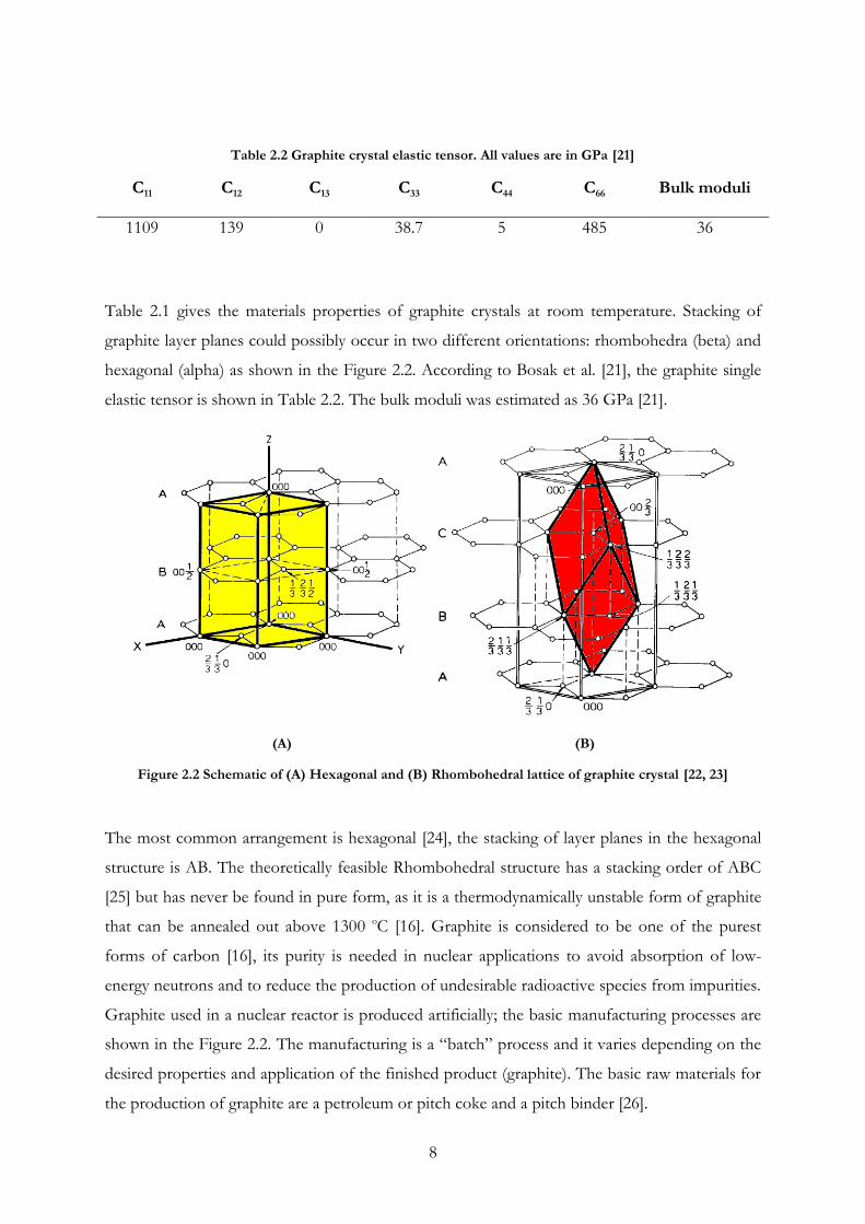
Figure 3.3 Schematic of the X- ray micro- tomography device adapted from Hall et al. [11] ......... 45
Figure 3.4 X-ray micro- tomography system used (X-Tek HMS- 320kV) ...................................... 46
Figure 3.5 Schematic diagram of stereographic projection (sample orientation is usually
expressed in terms of 2 Euler angles phi (Φ) and psi (ψ)) .................................................................. 49
Figure 3.6 Philips X’pert 1 goniometer.................................................................................................. 51
Figure 3.7 Texture analysis procedure (data regeneration) ................................................................. 52
Figure 3.8 Symmetric definition of Euler angles as spherical coordinates for a vector on the
surface of a unit sphere (adapted from [91]) ......................................................................................... 54
Figure 3.9 Helium Porosimeter ............................................................................................................... 55
Figure 3.10 Schematic diagram of helium porosimeter apparatus adapted from [104] .................. 56
Figure 3.11 PoreMaster series adapted from Quantachrome limited ............................................... 58
Figure 3.12 Big rig and Schematic of the whole big rig system ......................................................... 60
Figure 3.13 Picture and Schematic diagram of seismic velocity rig ................................................... 62
Figure 3.14 Piston assembly .................................................................................................................... 62
Figure 3.15 Sample assembling; A) component built by the author to protect the cables during
pressurization, B) sample with strain gauges attached, covered with heat shrink, C) the sample
jacketed to the loading piston, D) the sample was jacketed with heat shrink to the loading pistons
..................................................................................................................................................................... 64
Figure 3.16 Calibration for the pressure transducer, the voltage supply is 11.72V ......................... 67
Figure 3.17 Big rig force gauge calibration ............................................................................................ 67
Figure 3.18 P-P transducer Assembly Calibration ............................................................................... 68
Figure 3.19 P-S transducer Assembly Calibration ................................................................................ 69
Figure 4.1 X-ray diffraction spectrum for PGA ................................................................................... 75
Figure 4.2 Pole figures of the considered Gilsocarbon graphite sample, a) experimental figures
derived by the X-ray diffraction method, b) recalculated pole figures from ODF derived from
the experimental pole figures, c) difference between calculated ODF and the experimental data.
The set colour range in represent the intensity scales. The colour range have no unit, it was
denoted as multiples of uniform distribution (mud) values. It varies from 0 to 1.2mud for the
ODF derived ............................................................................................................................................. 76
Figure 4.3 Pole figures of the considered PGA (against grain) graphite sample, a) correction of
the experimental figures derived by X-ray diffraction data, b) recalculated pole figures from ODF
derived from the experimental pole figures, c) difference between calculated ODF and the
corrected x-ray data, d) Young’s modulus calculated from elastic tensor of a single crystal and
ODF. The colour range varies from 0 to 1.7 mud for the ODF derived......................................... 77
Figure 4.4 Tomography of Virgin PGA and Virgin Gilsocarbon (Gilso) ........................................ 79
Figure 4.5 Normalised PGA open pore volume entrance radius versus open pore volume ......... 80
Figure 4.6 Pore size distribution in Virgin PGA (B2, B4 and J18) and Gilsocarbon (A2, I11 and
I11b) nuclear graphite .............................................................................................................................. 81

xiii
Figure 4.7 Dynamic Young’s modulus (DYM) against total porosity in PGA-WG (PGA sample
parallel to the extrusion direction), PGA-AG (PGA sample against the extrusion direction) and
Gilsocarbon ............................................................................................................................................... 83
Figure 4.8 Shear modulus against total porosity in PGA-WG (PGA sample parallel to the
extrusion direction), PGA-AG (PGA sample against the extrusion direction) and Gilsocarbon. 84
Figure 4.9 Volumetric strain (V.S.) of PGA-WG- J4 and F1 during hydrostatic compression up
to 60MPa (dotted line) and 200MPa (solid line). The volumetric strain was changed from
negative strain to positive strain. The three stages (I, II and III) were explained in Table 4.2 ..... 85
Figure 4.10 Spring/frictional element diagram ..................................................................................... 87
Figure 4.11 Energy lost in the stress- strain curve of sample F1 ....................................................... 88
Figure 4.12 The history of axial, circumferential and volumetric strain during hydrostatic
compression of PGA with grain-J4 (dotted line) and PGA against grain-F4 (solid line) at 60 MPa.
A.A- Average axial strain, A.C- Average Circumferential strain, V.S- Volumetric strain .............. 89
Figure 4.13 Schematic diagram of PGA-WG and PGA-AG, the three dimensional schematic are
proposed by the author and the two dimension schematic are adapted from Eto et al. [118], .... 90
Figure 4.14 Volumetric behaviour of Gilsocarbon (E2), PGA AG (F5) and WG (F1) under
hydrostatic stress (200 MPa) states ......................................................................................................... 91
Figures 4.15 Gilsocarbon (E2) graphs of average bulk modulus against a) pressure and b)
porosity ....................................................................................................................................................... 92
Figure 4.16 PGA WG (F1) and AG (F5) average bulk modulus against confining pressure ........ 94
Figure 4.17 Total history of PGA-AG (F6) volume change during experiments (increase in
confining pressure, followed by axial deformation, and then confining pressure unloading) ....... 95
Figure 4.18 Schematic stress-strain curves for the confined axially symmetric shortening of
graphite ....................................................................................................................................................... 97
Figure 4.19 Axial deformation tests of PGA-WG (F2) (solid lines) and PGA-AG (F7) (dotted
lines) samples at CP of 60 MPa and both taken to maximum differential stresses of 50 MPa
(A.A. - Average axial strain, A.C. - Average circumferential strain, V.S. - Volumetric strain) ...... 98
Figure 4.20 Axial deformation tests of two PGA (AG) samples, one at CP of 60 MPa – F7 (solid
lines); maximum differential stress of 50 MPa and another at CP of 200 MPa – F6 (dotted lines);
maximum differential stress of 62 MPa (A.A.- Average axial strain, A.C.- Average circumferential
strain, V.S.- Volumetric strain). A and B represent the slope of the first and second axial loading
of F7. The test conducted using samples F6 and F7 are listed in Table 3.4 .................................... 99
Figure 4.21 Axial deformation tests of PGA-WG (J3) (solid lines) and Gilsocarbon (I2 as shown
in Table 3.4) (dotted lines) samples at CP of 200 MPa and both taken to maximum differential
stresses of 57 MPa (A.A. - Average axial strain, A.C. - Average circumferential strain, V.S. -
Volumetric strain) ................................................................................................................................... 101
Figure 4.22 Poisson’s ratios of two PGA-AG graphite samples (F7) at CP of 60 MPa and PGA-
AG (F6) at CP of 200 MPa during axial deformation ....................................................................... 102
Figure 4.23 Dynamic Young’s modulus with respect to the applied confining pressure on the
PGA-AG (J9) and PGA-WG (J23) graphite samples ........................................................................ 104
Figure 4.24 Dynamic Young’s modulus against the porosity change due to pressure effect on the
PGA-AG (J9) and PGA-WG (J23) graphite samples ........................................................................ 105
Figure 4.25 Dynamic Young’s modulus with respect to the applied confining pressure on the
Gilsocarbon graphite sample (I4) ......................................................................................................... 106

xiv
Figure 4.26 Dynamic Young’s modulus with respect to the applied cyclic confining pressure on
the PGA-WG (J23) graphite samples .................................................................................................. 107
Figure 4.27 Dynamic Young’s modulus with respect to the applied cyclic confining pressure on
the Gilsocarbon (I10) graphite samples ............................................................................................... 108
Figure 4.28 Shear modulus with respect to applied confining pressure on the PGA-AG (J15)
graphite samples ...................................................................................................................................... 109
Figure 4.29 Shear modulus against applied confining pressure on the Gilsocarbon graphite
sample (I5) ............................................................................................................................................... 110
Figure 4.30 Tomographic scans of Gilsocarbon (I8); (A) before and (B) after cyclic confining
pressure of up to 200 MPa. The red circled areas showed some of the regions where there was
porosity closure while the green areas showed some of the areas where crack opening was
noticed after deformation. ..................................................................................................................... 112
Figure 4.31 Frequency of the equivalent pore diameter of Gilsocarbon sample I8 tomography
scans before and after deformation ...................................................................................................... 113
Figure 4.32 Pore size distribution of virgin and deformed Gilsocarbon graphites (I1 –
hydrostatically loaded up to 200 MPa, I3 – hydrostatically loaded up to 200 MPa and differential
stressed up to 36 kN, and I7- hydrostatically loaded up to 80 MPa) .............................................. 114
Figure 4.33 DYM and shear modulus of Gilsocarbon against the Open Pore Volume (OPV)
before and after deformation at different loading modes (i.e. hydrostatic loading, differential
stress and dynamic loading) ................................................................................................................... 116
Figure 4.34 Pore size distribution of virgin and deformed PGA-WG graphites (J2 -
hydrostatically loaded up to 200 MPa and differential stressed up to 57 MPa, J22 - hydrostatically
loaded up to 200 MPa) ........................................................................................................................... 117
Figure 4.35 Pore size distribution of virgin and deformed PGA graphites (J8 - PGA-WG sample
hydrostatically loaded up to 200 MPa and differential stressed up to 74 MPa, J9 - PGA-WG
sample hydrostatically loaded up to 200 MPa) ................................................................................... 118
Figure 4.36 DYM and shear modulus of PGA-WG against the Open Pore Volume (OPV) before
and after deformation at different loading mode ............................................................................... 120
Figure 4.37 DYM and shear modulus of PGA-AG against the Open Pore Volume (OPV) before
and after deformation at different loading mode ............................................................................... 120
Figure 4.38 Pole to basal planes derived from the ODF calculated from the PGA experimental
pole figures before and after deformation. Colour scale is in multiples of uniform distribution.
................................................................................................................................................................... 121
Figure 5.1 Bulk modulus against porosity for the Voigt, Reuss, HS- and HS+ averaging schemes
compared with the experimental data for the Gilsocarbon sample (I3)–hydrostatically loaded up
to 202 MPa (loading data only). The I3 experimental data conform closely to the predictions of
Reuss and HS- averaging scheme. ........................................................................................................ 126
Figure 5.2 Bulk modulus against porosity of the KT model for the crack aspect ratio shown and
a zero-porosity modulus of 8.3 GPa, compared with the experimental data for the Gilsocarbon
sample (I3)–hydrostatically loaded up to 202 MPa (loading data only) .......................................... 127
Figure 5.3 DYM against porosity of the KT model for the crack aspect ratio shown and sphere
porosity compared with the experimental data for the DYM of PGA sample (J9) – seismic
loaded up to 202 MPa (loading data only) .......................................................................................... 128

xv
List of Tables
Table 2.1 Material properties of a graphite crystal at room temperature[20] ..................................... 7
Table 2.2 Graphite crystal elastic tensor. All values are in GPa [21] ................................................... 8
Table 2.3 Summary of Boey and Bacon results [49]; unirradiated graphite samples and Sleeve C
(Irradiated sample) .................................................................................................................................... 23
Table 3.1 Properties of PGA and Gilsocarbon nuclear graphites as reported by [83, 84] ............. 42
Table 3.2 X- ray Tomography scan settings .......................................................................................... 46
Table 3.3 XRD scan settings ................................................................................................................... 48
Table 3.4 The samples identities, directions and dimensions as well as the test done on each
sample ......................................................................................................................................................... 71
Table 4.1 Average DYM of the graphite ............................................................................................... 83
Table 4.2 Description of graphite inelastic and recovery behaviour using the volumetric strain
curve ............................................................................................................................................................ 86
Table 4.3 Change in Gilsocarbon elastic properties at different loading mode (i.e hydrostatic
loading, differential stress and dynamic loading) ............................................................................... 115
Table 4.4 Change in PGA elastic properties at different loading mode ......................................... 119
Table 5.1 Estimated elastic stiffness constants for pore-free, isotropically-textured polycrystalline
aggregates of the hexagonal crystals of Graphites A, B [125] and Graphite C (Single crystal
constants used in calculations are found in Bosak [21], estimated using equations from Toonder
et al. [126] and Berryman [125]). All units are GPa ........................................................................... 124
Table 7.1 Summary of data reported in the text for Gilsocarbon graphites ( K is the bulk
modulus, whilst K after is the bulk moduli after deformation E is the dynamic moduli, whilst E
after is the dynamic moduli after deformation, G is the shear moduli whilst G after is the shear
moduli after deformation). .................................................................................................................... 134

xvi
List of Abbreviations
AG Against grain
AGR Advanced gas-cooled reactor
CCD Charge coupled device
CT Computed tomography
CTE Coefficient of thermal expansion
DHP Digital helium porosimeter
DYM Dynamic Young’s moduli
EM Effective medium
Gilso Gilsocarbon graphite
HS Hashin-Shtrikman
KT Kuster and Toksoz
LPO Lattice preferred orientation
LVDT Linear variable differential transformer
ODF Orientation distribution function
PGA Pile Grade A graphite
PGA-AG Pile Grade A against grain
PGA-WG Pile Grade A with grain
TEM Transmission electron microscopy
VRH Voigt-Reuss-Hill
WG With grain
XRD X-ray diffraction
CPV Closed pore volume
OPV Open pore volume

xvii
List of Symbols
Mv Effective elastic modulus of Voigt bounds
MR Effective elastic modulus of Reuss bounds
μ1, μ2 The shear moduli of individual phases
E Young’s modulus
G Shear modulus
M P-wave modulus
υ Poisson’s ratio
K Bulk modulus
CH2 Methylene
C2H6 Ethane
H2S Hydrogen sulphide
H2 Hydrogen
CH3SH Methyl mercaptan
A Elastic compliance
σ Stress
B Material constant that characterises the plastic deformation.
ε Total strain
E Elastic modulus
P Porosity
Young’s Moduli of non-porous solid
Porosity
Ks The bulk modulus of solid
K air The bulk modulus of air (void)
Effective shear moduli of Hashin Shtrikman bounds
Effective bulk moduli of Kuster and Toksoz bounds

xviii
Effective shear moduli Kuster and Toksoz bounds
µ Absorption coefficient
λ Wavelength of electromagnetic radiation to the diffraction angle
d the lattice spacing of the lattice plane
n Integer
θ Incident angle
Euler angles
ψ Pole distance
Corrected intensity
Intensity from the random sample
Measured intensity from the texture sample
The pore radius
VL Compressional wave velocity
VT Transverse wave velocity
R The universal gas constant
T Temperature
n Number of moles
V Volume of the gas
P Pressure of the system
Vg Grain volume
Vb Bulk volume
VT Theoretical volume
VC Volume of the crystal
Vs Volumetric stress
F The frictional element
Ka Squashing spring
Kb The poroelasticity of the large pores

xix
Effective porosity percentage
Volumetric strain
Maximum compression direction

1
CHAPTER 1
1 Introduction
Artificially produced graphite as used in nuclear reactors is a porous (~20% porosity)
polycrystalline material. It can be classified as an engineering material with several advanced
applications, some examples of its use are:
in the steel industry, it is used an electrode material for arc furnace applications, the
anisotropy of graphites is one of the desired properties because it provides electrode with
adequate flexural strength along its length [1, 2].
the high electrical conductivity of graphite makes it desirable for use as electrodes and
brushes in electric motors as well as in solar energy applications [1]
while diamond is one of the hardest substance known, graphite is one of the softest.
Graphite can also be used for pencil and as a lubricant or coating to reduce friction and
corrosion [3].
graphite is suitable for use in rocket nozzles, due to its excellent thermal shock resistance
and,
in the nuclear industry, high purity graphite (nuclear graphite) is used within a reactor as a
moderator and reflector material, due to its low neutron absorption, and it is also an
excellent high temperature material [4].
It is the latter application, in particular the simulation of changes due to fast neutron irradiation
that the thesis is concerned.
Graphite bricks shrink when irradiated; pores and cracks are forced to close up to accommodate
the crystal expansion, and take up thermal expansion on the c-axis of the basal plane [5]. These
physical changes result in higher elastic modulus and strength of the material [6, 7]. Graphite
shrinkage could lead to disengagement of individual component and loss of core geometry.
Differential shrinkage in the graphite component can lead to the generation of internal stresses
and component failure by cracking. The latter behaviour is complicated by irradiation induced
changes in Young’s modulus and strength.
These dimensional and modulus change have been associated with the irradiation-induced
closure of many thousands of micro-cracks associated with the graphite crystallites due to crystal
dimensional change [8].
The aim of this work is to simulate the effects of closure of microcracks in nuclear graphite not
by irradiation but by external pressure, whilst measuring Young’s modulus, and to see if there are

2
any synergies between the changes in properties due to the two mechanisms (Hydrostatic
compaction and irradiation).
The harsh nuclear reactor environmental conditions (e.g. fast neutron fluence, radiolytic
oxidation and high temperatures) need to be accounted for when considering the structural
design and safety of core graphite structures. Safe design of graphite components requires full
understanding of the mechanical properties such as Young’s modulus, shear modulus and
Poisson’s ratio [7, 9].
The Young’s modulus of a nuclear graphite can be measured using two different methods i.e.
From the slope of the stress-strain curve close to the origin (tangent/secant/average
modulus)
The propagation velocity of an ultrasonic wave and the resonance frequency (dynamic
modulus).
The value of Young’s modulus calculated using these methods are not identical and there is
limited information on the relationship between the moduli obtained using these methods [7].
Extensive studies have been made in order to establish an understanding of the behaviour of
nuclear graphite under a variety of conditions, as well as to understand the structure-property
relationships governing the behaviour of artificially produced polycrystalline graphite [8, 10, 11].
Since irradiation changes are related to opening and closure of porosity and reorientation of the
crystallites in polycrystalline graphite, it is considered that an indication to the nature of these
changes may be gleamed by loading graphite under high hydrostatic pressure (up to 200MPa) as
a method of simulating crack closure. In the work reported here the effect of high pressure
(hydrostatic loading, differential stress and dynamic loading) on the static and dynamic moduli of
the nuclear graphite has been analysed and compared with each other. Mercury and helium
pycnometers have been used to measure the open porosity in each graphite sample before and
after hydrostatic loading. During testing the modulus was determined by monitoring the loading
and by using strain gauges and in some cases directly by ultrasonic measurement, in order to
investigate the effect of porosity distribution on static and dynamic modulus. In addition the
porosity of the samples has been examined before and after hydrostatic deformation using X -ray
micrography and is compared with the effective porosity distribution obtained using the mercury
pycnometry.
The relationship between experimental dynamic modulus and porosity change is compared with
literature data [12, 13] on the change in Young’s modulus of irradiated reactor graphite (Magnox
3
PGA and AGR Gilsocarbon graphite), in order to investigate relationship between the
hydrostatic compressed virgin samples and irradiated samples.
The research reported here combines measurement of mechanical properties of graphite under
high pressure and compares the experimental results with predictions made using various
effective medium models (Voigt, Reuss, Hill, Kuster and Toksoz, and Hashin-Shtrikman
bounds) previously developed to explain and verify the pressure/property relationships in other
materials (i.e. rocks and other porous materials). The effect of basal dislocation, surface energy,
porosity closure and heat lost during hydrostatic deformation were also considered. Helium and
mercury pycnometry was used to determine the porosity in loaded and unloaded samples. The
behaviour of graphite under the different loading conditions mentioned above was also analysed
and compared with each other.
This advantage of this approach to the investigation of crack closure in graphite is
the author did not have the expenses and difficulties associated with irradiating
specimens in a reactor or dealing with active material.
in this approach, the whole volume of graphite is altered during loading, and one can
examine the bulk property change, unlike in ion-irradiation where the irradiated volume
is minute, leading to difficulties in property measurement.
change in Young’s modulus can be measured in real time whilst the cracks are closing.
the experimental time scale is very short compared with irradiating samples.
differential stress can be applied at different initial hydrostatic pressures and hence crack
closure states.
From a scientific point of view graphite is an unusual material with extremely interesting
material properties; graphite properties and behaviour under loading is worthy of
investigation in its own right. Therefore this work is not only of interest to the nuclear
industry but it is an interest to science community as a whole
The design and safety assessment of nuclear graphite components is often based on empirical
rules derived from material irradiation data, but the accumulation of operational experience have
proven such empirical rules to be inadequate in some cases, therefore more understanding of the
relationship between change in microstructures and bulk mechanical properties is required [14].
The changes in graphite properties in a reactor are driven predominantly by fast neutron
irradiation (and radiolytic oxidation). Understanding graphite microstructural changes during

4
hydrostatic loading may help to reveal how the dimensional and property changes in graphite are
influenced as the internal porosity is closed by irradiation-induced crystal dimensional change

5
CHAPTER 2
2 Theory and literature review
2.1 Importance of nuclear graphite in a nuclear reactor
During operation, graphite in a nuclear reactor undergoes significant property changes due to the
nuclear reactor environmental conditions (i.e. fluence, radiolytic oxidation, high temperature).
These effects change the crystal properties and microstructure of nuclear graphite in a complex
manner. These property changes have been studied over many years [5]. Bulk graphite
mechanical property changes influence the reactor core lifetime integrity. In order to understand
the irradiation behaviour of bulk graphite, it is very important to understanding the behaviour of
graphite crystallites. Graphite shrinkage may lead to disengagement of individual component and
loss of core geometry; graphite expansion could lead to large forces between structures
(component generation of high stresses i.e. higher Young’s modulus) and component failure by
cracking. Two of the most important considerations in designing a graphite moderator that will
have a long life are designing for component integrity and design that will ensuring that changes
in graphite core geometry are acceptable. Both these design issues are affected by irradiation
induced dimensional change and changes to the thermal and mechanical properties [15]. Of
particular interest are irradiation induced to changes to Young’s modulus, which is also affected
by radiolytic weight loss.
2.2 Manufacture of nuclear graphite; PGA & Gilsocarbon
An understanding of graphite microstructure which is determined by the manufacturing process
is required, because this influence the quality and behaviour of graphite. In general graphite is an
allotrope of carbon [16] and has many applications varying from pencil lead to electrodes.
Nuclear graphite is used within a reactor as a moderator and reflector material (sustaining the
nuclear fission chain reaction). For this purpose high purity graphite (free from neutron
absorption material e.g. boron) is required. Nuclear graphite is also used for other features
related to reactor cores, such as fuel sleeves, spacer rings, and shield-wall protection. Graphite
was also chosen for use in a nuclear reactor due to its high thermal conductance and its high
strength at temperature [17]. Anisotropic extruded pure petroleum coke graphite called Pile
Grade A (PGA) was used in the construction of the early United Kingdom nuclear power

6
reactors (Magnox) while a much improved graphite called Gilsocarbon, a near isotropic moulded
graphite manufactured from Gilsonite coke (natural asphalt mined in Utah, USA) was used as a
moderator in the Advanced Gas-cooled Reactor [18].
2.2.1 Crystal and bulk physical properties of PGA and Gilsocarbon
The graphite crystal structure (as shown in the Figure 2.1) was first proposed in 1924 by John
Desmond Bernal [19]. Graphite consists of layered planes of carbon atoms, the layers are stacked
above one another in a staggered manner. The spacing between layers is approximately 2.3 times
the distance between the adjacent carbon atoms in a layer.
Figure 2.1 Crystal structure of Graphite showing ABAB stacking sequence and unit cell in Yellow (adapted from [16] )
The crystal lattice has two main axes: the three directions along the basal plane (a-axes) and the
direction perpendicular to the basal plane (c-axis). In each layer plane, the carbon atom is bonded
to three other neighboring carbons to form continuous hexagons. The covalent bonding
between two carbons is very strong (524 kJ/mol) and short in length (0.141 nm). The bonding

7
between layer planes is longer (0.335 nm) and weaker (7 kJ/mol) and is attributed to van der
Waals forces [5, 16].
Table 2.1 Material properties of a graphite crystal at room temperature[20]
Property Units Value
a-axis c-axis
Density g/cm3 2.267
Interlayer spacing 10-12 m 335
Mosaic spread ° 0.15
Electrical resistivity ohm-cm 40 10-6 0.01 to 1.0
Thermal conductivity watts/cm K 2 to 5 0.4 to 0.8
Thermal expansion K-1 (20-100°C) -1.5 10-6 27 10-6
Thermoelectric power -5 not available
Magnetic
susceptibility emu/g -0.3 10-6 -21 10-6
8
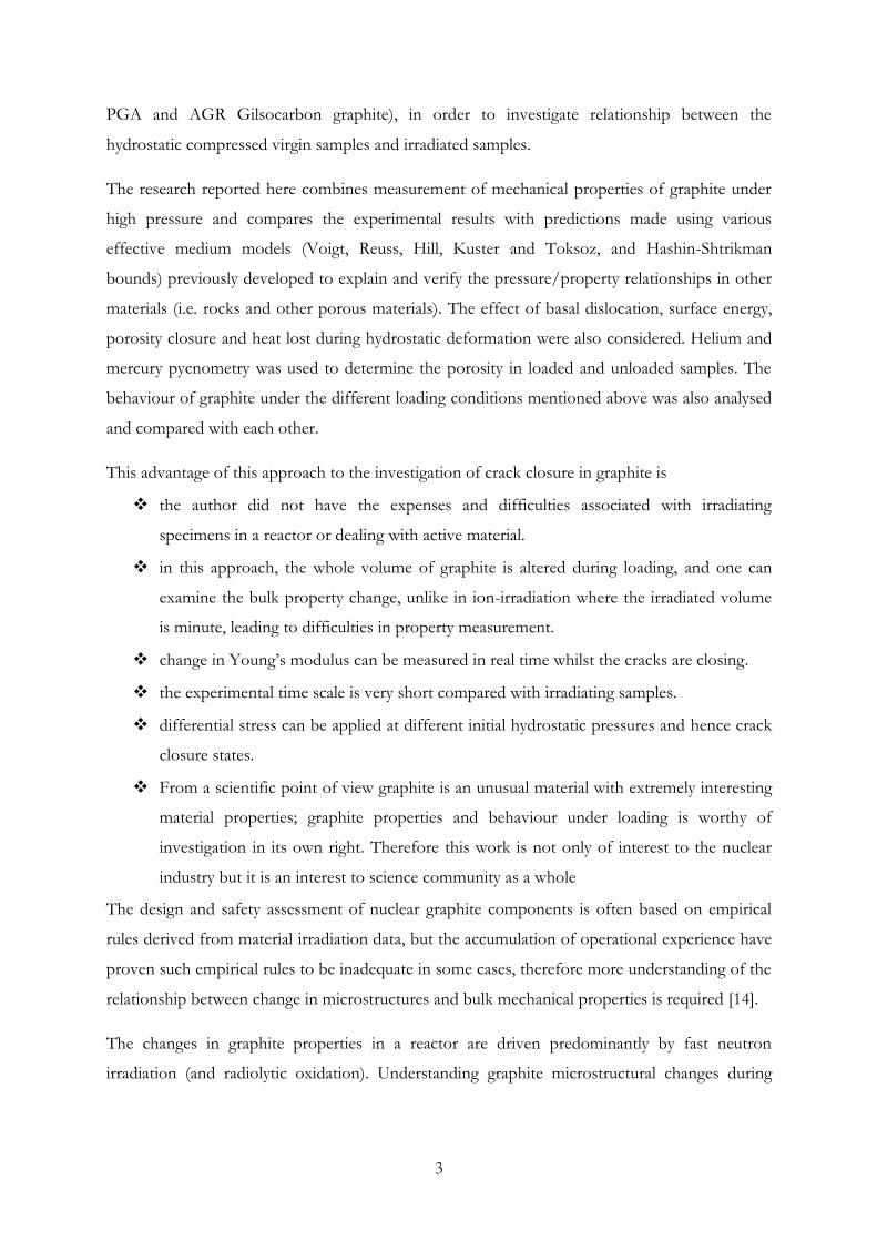
Table 2.2 Graphite crystal elastic tensor. All values are in GPa [21]
C11 C12 C13 C33 C44 C66 Bulk moduli
1109 139 0 38.7 5 485 36
Table 2.1 gives the materials properties of graphite crystals at room temperature. Stacking of
graphite layer planes could possibly occur in two different orientations: rhombohedra (beta) and
hexagonal (alpha) as shown in the Figure 2.2. According to Bosak et al. [21], the graphite single
elastic tensor is shown in Table 2.2. The bulk moduli was estimated as 36 GPa [21].
(A) (B)
Figure 2.2 Schematic of (A) Hexagonal and (B) Rhombohedral lattice of graphite crystal [22, 23]
The most common arrangement is hexagonal [24], the stacking of layer planes in the hexagonal
structure is AB. The theoretically feasible Rhombohedral structure has a stacking order of ABC
[25] but has never be found in pure form, as it is a thermodynamically unstable form of graphite
that can be annealed out above 1300 oC [16]. Graphite is considered to be one of the purest
forms of carbon [16], its purity is needed in nuclear applications to avoid absorption of low-
energy neutrons and to reduce the production of undesirable radioactive species from impurities.
Graphite used in a nuclear reactor is produced artificially; the basic manufacturing processes are
shown in the Figure 2.2. The manufacturing is a “batch” process and it varies depending on the
desired properties and application of the finished product (graphite). The basic raw materials for
the production of graphite are a petroleum or pitch coke and a pitch binder [26].

9
Figure 2.3: The manufacturing process for nuclear graphite (adapted from previous work [20, 25, 27])
The essential steps in the manufacturing process are: coke calcination, mixing, forming into
green shapes, baking and impregnation, and graphitising. In addition in some cases a final
purification step is required. The steps are outlined as follows:
Coke calcination: Petroleum coke is a by-product from the processing of crude oil
while pitch coke is manufactured from coal tar pitch or naturally occurring pitch.
Petroleum coke has a poor crystalline structure which can be improved through heating;
pitch coke structure is less ordered than petroleum coke. Coke is calcined prior to being
processed into graphite [25]. It is heated to 1300 0C during calcination in order to remove
any residual volatile hydrocarbons i.e. (methylene (CH2), ethane (C2H6), hydrogen
sulphide (H2S), hydrogen (H2) and methyl mercaptan (CH3SH) [28], resulting in a
materials volume reduction. The coke crystallinity is improved at the same time during
heating. In PGA and Gilsocarbon, the coke is produced from petroleum and Gilsonite
pitch respectively [29]. The calcined coke is crushed, ground and blended to obtain the
required filler particle distribution before mixing.
Mixing (the binder): Binder pitch is mixed with blended calcined coke. The binder is
either a petroleum or coal-tar pitch. Coal tar is a thermoplastic material; it is solid at
room temperature and it becomes viscous when heated. It is suitable as a binder for
graphite manufacture because of its high viscosity at high temperature, high carbon
content, high specific gravity, and because it is relatively cheap.

10
Forming into green shapes: After mixing, the aggregate is then allowed to cool before
being extruded or moulded into an artefact. The artefacts are of different sizes and
shapes, depending on the initial type of coke used and are termed the “green artefact”
although the article colour is not green. In PGA, the mixture is carefully extruded at
constant pressure and rate, resulting in a general alignment of the filler particles, which
are needle shaped, parallel to the direction of extrusion. The extrusion process gives rise
to an anisotropic bulk material, In Gilsocarbon, the mixture is moulded resulting in a
much smaller degree of directionality (alignment) of the filler particles. The degree of
anisotropy is also influenced by the size of the particle (i.e. 0.5 - 1 mm) and source of the
coke [25].
Baking and impregnation: The green artefact is baked at 1000 0C, where the remaining
volatile ash in the green artefact is removed and the pitch binder is carbonised. After
baking, the density of the green artefact is usually between 1.65 g/cm3 and 1.70 g/cm3.
The baked artefact is impregnated with pitch in order to increase the density and
improve the final material properties. A higher density can be achieved by repeating the
impregnation with a suitable pitch and then re-baking. The baking process leads to a
distribution of gas evolution pores in the structure of the final material [27, 28]
Graphitisation: Graphitisation involves a displacement and rearrangement of layer
planes and smaller groups of planes to achieve a three-dimensional ordering. Carbon can
be graphitised when heated at a temperature greater than 2500 0C in a furnace packed
with coke dust and silicon sand to prevent thermal oxidation. An high degree of
crystallinity is reached as the structure approaching a perfect crystal, resulting in changes
to the material properties. Graphitisation takes 3-4 days [20, 28].
Historically, the manufactured nuclear graphite’s density was 1.6-1.80 g/cm3. The density of
pure graphite crystal is 2.26 g/cm3 compared with the density of PGA (1.74 g/cm3) and
Gilsocarbon (1.81 g/cm3) [18, 30]. This suggested that both nuclear grades have ~20% porosity.
The lower density of PGA compared to Gilsocarbon is due to the differences in porosity
between the two nuclear graphite grades, which will be discussed later in this report.

11
2.3 Microstructural characterisation of nuclear graphite; PGA and
Gilsocarbon
The graphite article produced during graphitization consists of inter-connected filler grains and a
binder phase. This article is called polycrystalline graphite, due to the array of small
submicroscopic graphite crystallites making up the filler and the binder phases. Crystalline size
varies from 20-50 nanometer to a few microns in polycrystalline material [23, 31], their
orientations depend on the manufacturing process.
Polycrystalline graphite structure includes graphite crystal lattice, grain size and shape, the degree
of ordering within the tiny crystallites present in the polycrystalline phases, different pore size
distribution, and shape. Coke particle size varies between 25-300 μm [25, 32], the particle size
below 10 μm size are called flour [25]. In polycrystalline graphite, binder and filler are sometimes
indistinguishable. The nature of the binder-filler boundary, their shape and size is not well
understood. Filler particles consist of aligned crystallites and provide high strength to the
material [33, 34]. PGA nuclear graphite has distinguishable alignment of the filler particles.
PGA was manufactured for early gas-cooled reactors and the filler particles are derived from the
petroleum industries. PGA has an oval or needle-like shaped filler particle which is preferentially
aligned with the extrusion axis. The bulk material had anisotropic material properties since the
crystallites within the filler particle were preferentially aligned [10].
Gilsocarbon was manufactured for advanced gas-cooled reactors (AGRs) and the filler was
obtained from Gilsonite (naturally occurring asphalt mined in the USA). It has spherical, onion
shaped filler particles which have no preferential alignment during manufacturing process. The
bulk material had near-isotropic material properties, as the crystallites within the filler particle
tends to align circumferentially [10].
The filler particles in each graphite grade were highlighted with red mark as shown in the Figure
2.4. The black regions in the tomography are the porosity while the grey regions comprise the
graphite block.

12
Figure 2.4 Tomography images of PGA sample (J12) and Gilso (Gilsocarbon (I8)). The filler particles in each micrograph were marked in red
The binder and impregnated crystallites in both graphite grades are randomly oriented with no
preferential alignment. Extensive networks of interconnected pores, leading from the surface to
the core are also a common feature; these are referred to as ‘open pores’ as they are accessible to
gas or fluid. Isolated pores are referred to as ‘closed pores’ [35]. The manufacturing process
described above gives rise to a population of porosity and crystallite orientations in nuclear
graphite. Pore structures develop in the binder during the baking process. Binder can be
characterised by ‘domains’, which are regions of common basal plane alignment extending over
linear dimensions greater than 100 µm and ‘mosaics’ which are regions of crystallite disorderliness
with linear dimensions of common basal plane orientation of less than 10 µm [36].
2.3.1 Porosity in Polycrystalline Graphite
Previous work [4] investigated the porosity distribution in nuclear graphite and wide range
spectrum of pores was observed as shown in the Figure 2.5. Pores can be classified into three
families according to their size namely:
(a) micropores (very fine pores) < 2 nm,
(b) mesopores (fine pores) in the range of 2 nm - 50 nm and
(c) macropores (large pore) > 50 nm [37, 38].
The porosity populations can include gas evolution pores (micrometers in size), calcination
cracks (micrometers in width and tens of micrometer in length), and Mrozowski cracks
(nanometers wide and micrometers in length).

13
Figure 2.5 Mercury pycnometry result of pore size distribution in the nuclear graphite materials (adapted from Saheed [4])
Gas evolution pore: During the baking of the green artefact, gases and hydrocarbons
are driven off, resulting in cylindrical aspect ratio pores otherwise known as gas evolution
pores [39] They are sometimes referred to as open porosity, as they provide the route for
gases to penetrate into bulk structure.
Calcination crack: Calcination cracks formed during the coking process. They are large
cracks (few micrometers in length and width) and there are two types of this crack;
lenticular cracks which are aligned around the filler particle and non-lenticular cracks
from that crack through the layers. These crack populations are found in both nuclear
graphites, which will be discussed later in this thesis.

14
Figure 2.6 Transmission electron microscopy (TEM) image of nuclear graphite showing Mrozowski cracks (from Jones’s work [2])
Mrozowski cracks: These narrow cracks lie between the basal planes and arise from the
anisotropic shrinkage of the crystallites during cooling from graphitisation temperatures.
They are named after the author who first described their occurrence (Mrozowski) [40].
Typical Mrozowski cracks within Gilsocarbon graphite are shown in Figure 2.6. These
are important features in bulk graphite as during irradiation the crystals swell and result
in a closure of these cracks which affects to the bulk mechanical properties and cause
dimensional changes. Moreover their formation can also be linked with internal stresses
generated during cooling after graphitization.
At graphitisation temperatures above 2800 OC the thermal energy breaks the atomic bonds in the
structure and reform during cool down until the structure shocked. The high c-axis coefficient of
thermal expansion (CTE) results in local stresses with the structure. If there is a high local stress,
the structure has to accommodate for this and microcracks form. These align parallel to the
crystal c-axis [34, 39]. Mrozwoski cracks are present in the filler particle and binder. Mrozowski
cracks range from 10 nm in width and few nanometers to over 1 μm in length (example of
Mrozwoski crack show in Figure 2.7 [41].

15
Figure 2.7 crystal lattice showing Mrozowski crack
2.4 Mechanical properties and hydrostatic deformation of polycrystalline
graphite; bulk modulus, non-linearity and hysteresis behaviour - elastic
properties
Graphite is a weak and brittle solid material; compressive strengths are 3-4 times higher than the
tensile strengths [42]. The stress-strain behaviour is known for its non-linearity with load and a
hysteresis loop forms during cyclic loading, with permanent deformation on removal of applied
load. The uniaxial unconfined compression stress-strain relationships in polycrystalline graphite
have been widely studied in the past. Seldin [42] and Jenkins [43, 44] showed a non-linear stress-
strain curves similar to those shown in the Figure 2.7
2.8 ATJ graphite specimen stressed in compression (adapted from Seldin’s [42])
In uniaxial compression, the loading curve is convex upward while the unloading curve is always
concave downward with permanent sets formed at zero stress. The permanent set increases

16
when the previous maximum loading stress increases. Greenstreet et al. [1] also investigated size
effects and stress gradient upon the graphite material behaviour under flexural and uniaxial tests.
The size effects (volume and cross sectional area) were reported to be small or non-existent
within the size range investigated. Jenkins [45] relates graphite microstructural aspect to bulk
material behaviour by deducing a mechanical analogy for use in predicting stress-strain behaviour
in tension and compression. Elastic restraintt from the carbon network controls the extent of
plastic deformation experienced by the grain. The higher the stress, the less the restraint of this
network and more grains deform plastically. This carbon network allows non-linear deformation
even at very low strain. According to Jenkin’s model, the initial loading is described by
(2.1)
Where,
ε = total strain
A = Elastic compliance,
σ = Stress,
B = Material constant that characterises the plastic deformation.
The first part of the Equation 2.1 represents the elastic strain and the second part represents the
plastic strain. This general parabolic law fits the stress-strain curve fairly accurately at low stress
and strain rate [45]. At high stresses, Jenkin’s model deviates from the actual behaviour, probably
due to a reduction in apparent modulus, caused by an increased in microcrack density.
The properties of the polycrystalline materials are affected by porosity since 10-20 % of the total
volume is occupied by pores. There have been attempts to model the porous solid by relating
their bulk modulus to volume fraction of porosity. Spriggs [46] and Hasselman-Hashin [47, 48]
investigated the relationship between elastic Young’s modulus, E and porosity, P. The following
expressions were obtained respectively
(2.2)
(2.3)
Where K0 and E0 are the moduli of non-porous solid at a given stress (i.e. P = 0), b and c are the
empirical constants. Equation 2.3 was obtained for porous materials by Hasselman [47] from the
approximate expressions for bulk modulus (K) of heterogenous media derived by Hashin [48].
Hashin’s treatment is for closed pores while Spriggs equation is for total porosity in a volume of
solid. Boey and Bacon [49] assumed that K for coated (Jacketed specimen) and uncoated

17
(unjacketed specimen) graphite is determined by the closed and total porosity respectively.
According to Boey, the two equations above can only be applied to graphite, if it was further
assumed that the empirical form of Equation 2.2 may be applicable to K, that Equation 2.3
applies to anisotropic solids and that the constants b and c do not depend on the nature of the
porosity.
Brocklehurst et al. [50] investigated the effect of radiolytic oxidation on the properties of PGA
and isotropic reactor graphites for weight loss up to 35%. It was concluded that properties such
as thermal conductivity, Young’s modulus and strength were reported to decrease with weight
loss associated with increasing porosity (formation of microcracks).
Jenkins [51], Slagle [52], Oku and Eto [53] studied the formation or growth of cracks (increase in
porosity) in nuclear graphite during loading (bending, compression) and it was concluded that
there was an evidence for a buildup in crack density as original crack stabilized at pores and new
ones formed. Oku and Eto [53] suggested that crack growth becomes more evident around 60 %
of the compressive failure stress. It was also reported that the effect of pre-stressing shown a
decrease in Young’s modulus. The closer the stress approaches a critical value, the greater the
probability of localised crack formed, hence the greater the decrease in Young’s modulus. Hall
[11] noted that the fall in Young’s modulus value at low pre stress level is due to an increase in
dislocation density which would recover completely following thermal annealing treatment.
2.5 Hydrostatic deformation investigation
Since the aim of this work is to develop an investigation of graphite response to hydrostatic
loading, previous work by Paterson and Edmond [54], Boey and Bacon [49], Kmetko et al. [55]
and Yoda [56] were investigated to other to establish the facts and assumption about graphite
microstructural changes and there relevance to the authors research.
2.5.1 Paterson and Edmond’s work
Paterson and Edmond [54] studied large uniaxially symmetric deformation of porous
polycrystalline graphite (electrographite grade EY9) at high pressure. The specimen is enclosed
during the test in a dilatometer which fits inside pressure vessel and permits simultaneous
determination of volume change and stress/strain characteristics. This genius method is the
pioneer of its kind. High hydrostatic pressure applied prior to differential stress suppressed
deformation by growth of dilatant and microcracks. According to Paterson and Edmond, the
large deformation might help in understanding the mechanisms of deformation of graphite. High

18
pressure experiments showed that the compression stress-strain curve of a polycrystalline
graphite depended upon the applied confining pressure (1-8 kbar) [54]. In the work of Paterson
and Edmond, volume changes occur during deformation as well as during application of
pressure. There is almost complete recovery of length and volume during the release of pressure
after 20% strain.

19
Figure 2.9 Total history of volume change during multiple high hydrostatic pressure cycling (Paterson and Edmond [54]). The elastic line represents the behaviour expected from single crystal compressibility
modulus. The high pressure deformation apparatus used consists of a pressure vessel containing a fluid medium into which piston was introduced to apply a superimposed axial load to the specimen
Figure 2.10 A) Compression stress-strain curves and B) Volume change during deformation at confining pressures from 1 – 8kb. The scatter represents the error bar
In the Figure 2.9, the volume of the graphite changes at various pressures. Each stage of the
volume change was described as follows.

20
Volume decrease as confining pressure increases.
During the 20 % straining, volume decreases further at fixed confining pressure.
Slight increase in volume on removing the differential stress (same confining pressure) as
shown in Figure 2.10B.
Large increase in volume during release of confining pressure, this recovers almost the
initial volume, mainly below 0.5 kb
Above 1 kb, there is also length recovery, final length of the specimen is 1-2 % shorter than
initial length. Paterson concluded that
The stress strain curves (shown in Figure 2.10A) show strong dependence on pressure.
Assumes that the deformation is due to sliding of granular particles against the resistance
of macroscopic friction.
When the high pressure is released the internal stresses are relived resulting in high strain
recovery.
The deformation may also accompanied by ‘flexure of platelets’ which could also
introduces the internal stresses responsible for recovery effects.
Opening of new cracks and pores during pressure release may also contribute to the
recovery effects, including giving rise to additional volume recovery
2.5.2 Boey and Bacon work
According to Boey and Bacon [49], polycrystalline nuclear graphite density is less than that due
to graphite crystals alone due to the presence of porosity which has implications for the bulk
compressibility. The work of Boey and Bacon [49] was to investigate on unirradiated and
irradiated deformation behaviour of several graphites under a gas pressure up to 4.14 MPa (600
psi) and the effect of increasing the closed porosity on hydrostatic deformation of graphite.
Boey and Bacon [49] hydrostatically deformed various uncoated and coated virgin Gilsocarbon,
PGA moderator graphites and pitchcoke (fuel sleeve graphite). The results are shown in Figures
2.11 and 2.12, (the symbol (l) represents a sample cut in the longitudinal direction while (c)
represents samples cut in the circumferential direction). Both virgin coated and uncoated
graphite samples exhibit linear pressure strain relationship. There was reduction in strain in the
uncoated specimen for a comparable pressure compare to coated sample, Boey and Bacon
concluded that the coated specimens are stiffer that uncoated specimens [49].

21
Figure 2.11 Pressure versus strain for uncoated specimens of virgin graphite (adapted from Boey and Bacon [49])
Figure 2.12 Pressure versus strain for coated specimens of virgin graphite (adapted from Boey and Bacon [49])

22
The result for the hydrostatic deformation of uncoated irradiated fuel sleeve graphite is shown in
the Figure 2.13. These irradiated uncoated specimens exhibit a non-linear pressure/strain
relationship and large hysteresis looping behaviour is exhibited.
Figure 2.13 Pressure versus strain for uncoated specimens of graphite irradiated to a neutron dose of 7, 11, and 17x1020n/cm2 in circumferential (c) and longitudinal strain (l) directions (adapted from Boey and
Bacon [49]).
It was noted that the circumferential loops were generally larger than those observed in the
longitudinal direction, but in Graphite irradiated to neutron dose 11x1020n/cm2, the
longitudinal strains was slightly larger due to the fact that the specimens were machined in the
circumferential from the sleeve material.
In the irradiated samples there is a reduction in strain for a comparable pressure compared to
unirradiated samples, implying that the irradiated graphite is stiffer than unirradiated graphite.

23
Table 2.3 Summary of Boey and Bacon results [49]; unirradiated graphite samples and Sleeve C (Irradiated sample)
A summary of Boey and Bacon [49] values for Young’s modulus E and Poisson’s ratio υ
obtained from static uniaxial tests are given in the Table 2.3. There is considerable variation in
bulk modulus K between graphites. The value for sealed graphite is reduced significantly. The
bulk modulus (K) for irradiated sample is higher than for the virgin samples as shown in the
Table 2.3. Boey and Bacon suggested that the elastic changes were due to the changes that took
place in the graphite microstructure, which contains spectrum of pores inherited in the raw
material or arise from the graphite manufacturing process. Boey and Bacon concluded that
K is reduced when graphite sample is sealed.
Under uniaxial loads, all pores can assist in accommodating normal and shear
deformation thereby contribute to E and υ, which correspondingly reduced.
Under fluid pressure, deformation in open porosity is restricted because of its
accessibility to fluid, closed micropores shrink, K decreases.
Microcracks present in the grains reduce the restraint on plastic deformation that
crystallites experience due to their neighbours while macropores within the binder phase
can accommodate the shear deformation of individual particles.
2.5.3 Study of Kmetko et al. [55]
Kmetko et al. [55] studied the hydrostatic compression of synthetic polycrystalline graphite
(AUC graphite) and the effect of pore structure accessibility. The sample was studied under two
conditions:

24
sealed in a 2-3 mm thick copper jacket to prevent confining fluid (pentane) penetration
into the graphite pores
not jacketed, to allow fluid penetration.
The length change was measured with dilatometer located inside the pressure vessel, the result
from the two conditions are significantly different to each other as shown in the Figure 2.14. The
displacement observed in the jacketed sample is non-linear and has a larger magnitude compared
with the unjacketed sample. In the unjacketed sample, the compressive stress was applied to
individual crystallites comprising rigid cross-linked of solid. In the jacketed sample, the
hydrostatic stress was applied to the outside boundary of the graphite therefore the whole
microstructural (crystallite network including porosity) was compressed, leading to large strain of
jacketed sample as shown in the Figure 2.14.
Figure 2.14 Displacement of AUC graphite along the extrusion direction during hydrostatic compression (adapted from Kmetko el al. work [55])
Kmetko et al. concluded that:
The difference in behaviour is attributed to the effect of porosity of the AUC graphite.

25
Graphite experienced slight deformation when unjacketed but grossly deformed when
jacketed and subjected to pressure.
It was estimated that the total volume decrease of 30 % below 600 MPa suggested that
virtually all of the porosity has been closed.
The coefficient of thermal expansion (CTE) is estimated to be ~0.4 greater perpendicular
than parallel to its direction of extrusion [55, 57].
The compressibility of unjacketed graphite sample is 0.35 times that of the jacketed
materials in its densified state above ~600MPa. This value is approximately the fraction
of the volume CTE for AUC graphite to that of the single crystal which is in agreement
with the assumption that the structural sensitivities of thermal expansion to that of
compressibility are similar.
Hydrostatic deformation changes polycrystalline graphite’s macroscopic dimensions in a
similar manner to the thermal contraction of the aggregate
2.5.4 Work from Yoda et al. 1984
The aim of the Yoda et al. [56] work was to understand the characteristics of ISO-20 and IG-11
polycrystalline graphite under hydrostatic stress. These are fine-grained isotropic graphites
manufactured by Toyo Tanso limited. The samples were hydrostatically loaded in a piston-
cylinder type pressure apparatus up to a maximum confining pressure (fluid medium) of 600
MPa. ISO-20 was subjected to 2 cycles while IG-11 was subjected to 3 cycles, and the change in
observed axial elongation as the pressure increases are shown in the Figure 2.15. During the first
cycles the total deformations at the unloading and reloading points increased with increased cycle
number, indicating that there was a slight increase in the apparent density during cycling.
ISO-20 seems to be stiffer than IG-11, Yoda et al. suggested that this behaviour might be due to
the high density and unconfined compressive strength (1.90 g/cm3, 140 MPa respectively) of
ISO-20 compared to that of IG-11(1.75 g/cm3, 80MPa respectively).
The relationship between the axial strain and volumetric strain for large strain deformation of an
isotropic solid was considered. The large strain ( ) is ~ 0.05, the quadratic elongation ( ) could
be written as (1+ )2 or ( )2 . The volumetric strain was calculated as 0.156 using the quadratic
elongation equations. For small strains (where 2 « ) the volumetric strain is calculated as 0.15
by adding . The difference between the two calculated volumetric strains is small
(0.006).

26
Figure 2.15 Hydrostatic pressure versus observed strain curves showing deformation behaviour of IG-11 and ISO-20 (adapted from previous work [56])
Yoda et al. [56] concluded that
The concave shape of the curve at higher pressure would be identified by the shrinking
of pores in the graphites caused by the pressure [56].
At high pressure, the graphite is expected to behave as a hypothetical graphite without
pores.
2.5.5 Basis of the author’s work
Although all the previous work suggested that closure and opening of cracks play a major role in
the non-linear and hysteresis loop behaviour of graphite under hydrostatic loading, none of the
previous work analyses the contribution of porosity sizes to the graphite behaviour. Even though
Boey and Bacon [49] analysed the total porosity change before and after deformation but the
effect of porosity sizes were unknown which made it difficult to understand which porosity size
scales (micopores or macropores) have the major effect on graphite behaviour under load. It is
considered by the author that the knowledge of pore size distribution will help to reveal the
dominant features in the graphite microstructure, whether the binder which has high
concentration of both micropores and macropores or the filler particles that have high

27
concentrations of microcracks. Moreover the internal microstructural changes before and after
hydrostatic deformations were not examined by previous work. In the present study, highlights
regions of interest in the graphite micrograph before and after deformation are highlighted. The
effect of hydrostatic pressure on crystallites is also examined.
2.6 Effect of irradiation on elastic property changes in nuclear graphite
Carbon and graphite have been widely used as structural materials for the high temperature
environment (furnace, nuclear reactors and aerospace), due to their superior toughness at high
temperature. The elastic modulus and strength of nuclear graphite increase with temperature [12,
58], the elastic modulus shows maximum value at 1800 OC, while the tensile strength reaches
maximum around 2500 OC above [59]. Characterisation of the mechanical properties (i.e. elastic
moduli) of graphite is fundamental to determining the induced and applied stresses on the
graphite components in a reactor. Determining the resulting stress within and around the
graphite component from the exposure to a reactor environment is necessary to estimate the
ability of graphite to withstand the imposed loads and continued service conditions. Therefore it
is paramount to develop a database of the properties for a given graphite grades (i.e. PGA and
Gilsocarbon).
2.6.1 Fast neutron effect
Fast neutrons produced by the fission process in a reactor collide with the nuclei of carbon
atoms (primary atoms) in the graphite moderator and transfer energy to them. If the bonding
energy of the carbon atom in the lattice (≈ 5 eV ≈ 500 KJ/mol) is less than the energy of
energetic neutron, primary atoms will be knocked out from the lattice and collide with another
atom causing further displacements and projectiles in a cascade effect through the crystal as
shown in Figure 2.16 [58].

28
~0.01 m
Vacant lattice site
Interstitial atom
1 keV
0.001 m ~500 eV
Figure 2.16 Schematic of displacement cascade in graphite crystal (adapted from [20, 58])
The initial collision between a carbon atom and a neutron produces a large number of
displacements in the form of either interstitial carbon atoms and/or vacant lattice defects.
Interstitial defects may form when an atom occupies a position between normal lattice positions,
and vacancy defects occur where atoms have been removed from its lattice position. Previous
works [5, 60] have proposed damage mechanisms of neutron irradiation in graphite crystals.
It was suggested [5] that the vacant lattice sites can be considered to be stable while the
interstitial atoms move in between the basal planes. Violent thermodynamically stable
concentration of thermal produced defect, it was previously proposed that large numbers of the
mobile interstitial atoms might recombine with the vacant lattice sites (annihilation) [5] while
some of them combine with one another to form small interstitial groups or clusters with a
stable size of 4 ± 2 atoms. The interstitial groups may collapse under further neutron irradiation.
The size and number of these interstitial groups that can be formed is a function of temperature,
speed of transport through the graphite crystal and time. As the temperature is increased, the
groups can potentially form bigger clusters and the group quantity is reduced. Moreover it was
suggested that vacancies can be filled without interstitial annihilation resulting in increased lattice
strain [58]. This lattice strain damage mechanism causes significant structural (i.e. dimensional
changes) and property changes (i.e. elastic moduli) to graphite [61]. These damage mechanism
above is postulated to cause crystal growth perpendicular to the basal plane (c-axis direction)
whereas shrinkage parallel to the layer planes (a-axis direction) is said to be due to vacancy
formation, Poisson’s ratio effect and c-axis expansion [39, 60, 62]. Since the polycrystalline
graphite consists of random orientations of filler particles and crystallite cracks and porosity,

29
polycrystalline graphite dimensional changes are governed by the irradiation - induced changes in
the crystallites and interaction of porosity with the crystallites [61].
In polycrystalline graphite, there is initial expansion in the crystallographic c- direction due to
interstitial defect formation and shrinkage in the a- direction due to coalescence of vacancies,
hence graphite net volume shrinkage is observed [61]. During neutron irradiation, the cracks and
pores start to close up in order to accommodate crystal expansion in the c-axis. These physical
changes are postulated to result in higher elastic modulus and strength of the material [61]. The
Young’s modulus of irradiated graphite may be increased by three times its value before neutron
irradiation as shown in Figure 2.17. Accumulation of new pores at high dose is thought to reduce
the strength and modulus [61]. In Figure 2.17, increasing the temperature to 600 OC increases the
rates of the second increase and of the decrease, but the maximum Young’s modulus reduces
slightly. It was also noted that the dose at which the Young’s modulus decreases also reduces
with increasing temperature [34]. Graphite strains by localized slipping of the basal plane. At
lower dose, the pinning of dislocations suppresses anelastic behaviour causes an increase in
Young’s modulus. This is otherwise known as irradiation stiffness. The effect on Young’s
modulus is known as “pinning”. Further increase in Young’s modulus after irradiation stiffness
due to pinning is attributed to structural tightening due to crystal swelling or crystalline
deformations. This behaviour is referred to as a structural effect. Eventually, the DYM falls with
further increase in dose due to generation of cracks within the microstructure associated with
weight loss caused by radiolytic oxidation
Other work [5, 6, 60] on irradiation behaviour of nuclear graphite concluded that volumetric
changes were similar to the changes mentioned above (initial densification followed by a rapid
expansion). As the neutron flux increase, this densification increases until all the pores were
exhausted and the c-axis expansion of the crystallites was able to be transmitted to the bulk
material. This signified the beginning of the expansion phase where a large porosity formed
between the filler particles at high doses and accounted for the large volume expansion of the
graphite.

30
Figure 2.17 The effect of fast neutrons on the Gilsocarbon Young’s modulus (adapted from [34])
Figure 2.18 The effect of thermal cycling (between ambient temperature and 1100OC) on the DYM of Gilsocarbon (transfers direction). The solid line represents heating while broken line represents cooling
(adapted from [63])

31
A well known characteristic of polycrystalline graphite is that the elastic modulus rises with an
increase in temperature, for temperatures well above room temperature (i.e. 250-300 OC) [64]. As
the temperature increases further (>~250 OC), the modulus increases up to 10 %. This might be
associated with tightening of the graphite structure and closure of porosity. Thermal cycling
showed that after heating up to 1100 OC and cooling to ambient temperature, the modulus
decreased slightly by 1 %.
The changes in Figures 2.17 and 2.18 have been related with mechanisms such as crystallite
swelling, formation and closure of porosity, pinning (pinned dislocations in the basal planes) in
the case of irradiation and tightening of the graphite structure [20].
2.6.2 Oxidation effects
Several studies have been made of the relationship between the graphite pore structure and their
oxidation characteristics [34, 50, 65-67]. In graphite moderated reactor cooled by carbondioxide
(CO2), some degree of graphite oxidation will occur. The gas contained in the open pores of the
graphite material absorbs radiation energy (gamma radiation), causing CO2 to breakdown into
active species (CO2*) which attack the graphite material (pore surface) as shown in the Equation
2.4. This process is called radiolytic oxidation. It adversely affects the physical properties of
graphite and results in the enlargement of existing pores. The knocked-out carbon atoms in
graphite leave vacancies, which can then be enlarged by reacting with the carbon atoms in the
gaseous phase. According to previous work [50, 65] the most noticeable effect of oxidation on
graphite microstructure is the enlargement of the pores caused by reaction of carbon atoms of
the solid material with the oxygen molecules of the gas phase.
(2.4)
The density of oxidized graphite is altered by enlargement of existing pores, new pores
generation, and development of micro failure. Radiolytic oxidation occurs uniformly throughout
the specimen and this removal of materials from the internal surfaces affect the physical
properties of the graphite [50].
Radiolytic corrosion can be controlled by the addition of methane inhibitor to the CO2 coolant.
Methane protects graphite by forming a carbonaceous film on the surface of the pore, corrosion
becomes increasingly inhibited to low surface area pores. In the recent AGRs, the use of
improved near-isotropic Gilsocarbon as the moderator readily controlled the corrosion to an

32
acceptably low rate, due to low open porosity volume (~0.10 cm3/cm3) compared with PGA in
the Magnox station which has higher open pore volume (~0.21 cm3/cm3) [50].
Kelly et al. [6, 68] report on thermal annealing of irradiated graphite shows that it is possible to
remove the effect of the small interstitial and vacancy groups to the extent that Young’s modulus
is covered to the unirradiated (original) value. However the annealing does not return graphite
microstructure to its original state but changes the configuration of the defects (interstitial,
vacancy etc.) so that they no longer influence the physical properties of Young’s modulus. Kelly
et al. [69] reported the mechanical property (Young’s modulus) changes for irradiated
Gilsocarbon after neutron irradiation damage annealing by heat treatment. Spriggs’ [46] and
Knudsen’s [14, 70] equations were expressed in term of changes in Young’s modulus E, and it
was reported as follows
(2.5)
Modulus of non-porous solid is represented with , the effect of radiolytic oxidation on nuclear
graphite was simulated by Brocklehurst and Adams [12], this was achieved by drilling different
arrangement of holes in the graphite samples. These samples were tested to determine their
mechanical properties for weight losses ranging from 0 to 50%. The effect of increasing
simulated oxidation on Young’s modulus was reported as:
(2.6)
The changes in the Young’s modulus were lower in the drilled specimen than the Young’s
modulus of real radiolytic oxidised graphite by a factor of 1.3 [12, 13]. The difference between
these two Equations (2.5 and 2.6) is shown in Figure 2.19

33
Figure 2.19 Change in Young’s modulus associated with weight loss (adapted from [12, 13])
The complex physical and mechanical properties changes seen in neutron induced radiolytic
oxidised graphite are not fully understood. Since the mechanism of porosity closure and
formation and crystal growth have been associated with the irradiated graphite property change,
these mechanistic behaviours of irradiated graphite can be simulated by deforming virgin
graphite hydrostatically using a high pressure rig. Studying the changes in virgin graphite
microstructure as a result of different loading modes might help to gain an understanding of
complex physical and mechanical properties of irradiated graphite.
2.7 Deformation of graphite under high hydrostatic pressure
According to Seldon [42], the effect of externally applied stresses within the crystallites can lead
to a combination of elastic deformation, irreversible shear and plastic deformation, internal stress
relief and local stresses which can produce microcracks. The elastic and plastic deformation
y = e-2.7x
y = e-3.6x
0
0.2
0.4
0.6
0.8
1
1.2
0 0.1 0.2 0.3 0.4 0.5
Rela
tive
Yo
un
g's
mo
du
lus,
E/
EO
Porosity
Drilled
Oxidised
Expon. (Drilled)
Expon. (Oxidised)

34
effects are used to describe the stress against strain behaviour of graphite while the other effects
mentioned are used to describe the stress against strain curve in different directions.
The hydrostatic deformation behaviour of nuclear graphite is in a way different to uniaxial
compression. Both open and closed pores presences in graphite microstructure have different
effects on the way the graphite deforms under different modes of loading (i.e. uniaxial and
hydrostatic loading). In order to understand the effect of these loadings on the graphite
microstructural changes, it is necessary to understand the microstructures of the polycrystalline
aggregate consisting of a few particles as shown in Figure 2.20 (graphite microstructure optical
image) and schematically in Figure 2.21.
Figure 2.20 Optical image of PGA graphite
During baking, the coke particles support each other until the binder is solidified (filler particles
are supported by binder matix); therefore the particles are always in close contact with each
other, linked by bridges of coke binder. The shrinking binder does not provide a high density
shell around each particle, hence the binder layer is full of microcracks perpendicular to the
surface of the particles.
Macropores appear in between the particles and also spread throughout the binder phase. The
crystallites within the coke are all nearly parallel. They are microcracks formed within the

35
crystallites due to differential thermal contraction and disorientation of these crystallites. It can
be concluded that the coke grains are full of pores and cracks.
Figure 2.21 Typical detailed microstructure of graphite (adapted from [71])
Under uniaxial loading both open and closed porosity behave in the same manner, the porosity
provide space for accommodating shear deformation of the coke particles, contributing to the
overall deformation of the porous aggregate [42, 49]. The strain observed during uniaxial
deformation should be higher than the strain observed during hydrostatic deformation due to
the presence of major shearing of the coke particles into the open porosity.
Under hydrostatic loading of graphite, porosity allows crystallites to deform by shear motion of
the layer planes, producing shear stresses which can induce plastic flow [49]. Individual particles
are suspected to be accessible by pressure fluid, due to the existence of open pores in the binder
phase as well as several cracks in the binder layer surrounding the coke particles. During
compression, the coke particles compressed and shear also occurs at the same time. The
confining pressure compressed the grains into each other resulting to dilatation of individual
particles/grains. This is demonstrated in the Figure 2.22 by the same particles shown
schematically in Figure 2.21.

36
Figure 2.22 Schematic diagram of applied hydrostatic pressure
In polycrystalline graphites, the population of the mobile plane dislocations is greater than in the
single crystals due to large population of twin and tilt boundaries between and within crystallites
[72]. According to Boey and Bacon [49], the shear deformation of the coke particles into the
surrounding pores is responsible for the apparent low value of Poisson’s ratio for the
polycrystalline materials. The closed pores between the particles can contribute to the hydrostatic
deformation of the graphite by accommodating the internal strains in the particle.
2.8 Using theoretical models to estimate effective medium moduli
Effective medium theories have been developed in the previous work [73-77] to estimate the
effective medium moduli of polycrystalline solids (i.e. rock, graphite etc.) in terms of the
properties of various constituent minerals and pore fluids. To achieve this, the following must
me incorporated
The individual elastic moduli of the constituents
The volume fractions of the constituents
Geometric details of how the constituents are arranged
Since the geometric details of the constituents of a polycrystalline solid are quite challenging to
measure, boundary methods have been adapted to estimate the effective moduli of the
polycrystalline solid by estimating the upper and lower bounds on the moduli. The bounds
models are one of the types of theoretical models that are relatively free of assumptions about
the material microstructure and give rigorous upper and lower limits on the moduli, given the
composition. The theoretical models used in this work are Voigt-Reuss-Hill bounds (VRH),
Hashin-Shtrikman bounds (HS), and Kuster and Toksoz models (KT).

37
2.8.1 Voigt-Reuss-Hill bounds (VRH)
The Voigt and Reuss averages are interpreted as the ratio of average stress and average strain
within composites [74]. The upper bound (Voigt) and lower bound (Reuss) are found assuming
that there are uniformity in strain and stress respectively throughout the whole composite. The
Voigt upper bound and Reuss lower bound of the effective elastic, modulus, Mv, of N phases are
∑
(2.7)
∑
(2.8)
Where fi is the volume fraction of the ith phase,
Mi is the elastic modulus of the ith phase and
Mv and MR are the effective elastic modulus of Voigt and Reuss bounds respectively
represents fraction
Ks and K air are the bulk modulus of solid and air (void)
The Voigt-Reuss-Hill average is the average of Voigt upper bound and the Reuss lower bound as
shown in Equation 2.9
(2.9)
This method assumes that each constituent is isotropic, linear, and elastic. It is commonly used
in estimating rock elastic properties.
2.8.2 Hashin-Shtrikman bounds
The Voigt-Reuss bounds are wider than Hashin-Shtrikman (HS) bounds. This bound is the
narrowest possible bound on moduli that can be estimated for an isotropic material, knowing the
volume fractions of the constituents. When there are only two constituents, the bounds are
written as;
( )
(2.10)

38
( )
(2.11)
Where K1 and K2 are the bulk moduli of individual phases; μ1 and μ2 are the shear moduli of
individual phases; and f1 and f2 are the volume fractions of individual phases. The upper (HS+)
and lower (HS-) bounds are computed by interchanging which material is termed 1 and which is
termed 2. When the stiffest material is termed 1, the expressions yield the upper bound and the
lower bound when the softest material is termed 1. Like the VRH model, this method also
assumes that each consistent is isotropic, linear, and elastic. It is used in estimating rock elastic
properties.
Figure 2.23 Bulk modulus curves for Calcite rock with water using effective medium theories (adapted from[78])
Distance between upper and lower bounds depends on difference between the end member
constituents. Bulk moduli of Calcite and water are 7 GPa and 2.2 GPa respectively as shown in
the Figure 2.23, the mixture of Calcite and water gives widely spaced bounds. The HS- and
Reuss bounds are identical. The Voigt bound is more stiff than other bounds.

39
2.8.3 Kuster and Toksoz models (KT)
Kuster and Toksoz [73] derived expressions for P- and S-wave velocities by using a long-
wavelength first-order scattering theory. Their formulation can be used to calculate effective
moduli for randomly distributed inclusions [73, 77]. A generalization of the expressions for the
effective bulk moduli and shear moduli can be written as
( )
(
)
∑
(2.12)
∑
(2.13)
(
) (2.14)
Where the ,
are the effective bulk and shear moduli respectively for a variety of
inclusion shapes. The coefficients and describe the effect of an inclusion of material, i
in a background medium, m, while is the volume concentration of the inclusion, is the
fraction of effective bulk and shear moduli. Inclusion shapes include spheres, needles, disks and
penny cracks.
According to previous work [74], for spherical inclusions, the KT expression for bulk modulus
are identical to the HS upper bound, even though the KT expressions are formally limited to low
porosity. KT formulation assume
isotropic, linear, and elastic media;
limitation due to dilute concentrations of the inclusions; and
idealized ellipsoidal inclusion shapes.
Since Gilsocarbon is near-isotropic graphite, it was suggested that these theoretical models
(VRH, HS+, HS-, and KT) can be used to validate the experimental results (behaviour of
Gilsocarbon under hydrostatic pressure) by comparing the effect of porosity on effective bulk
moduli. The comparison between experimental curves and the theoretical models is discussed
further in Chapter 5.

40
2.9 Conclusion
The deformation behaviour of polycrystalline graphite differs from that of a single crystal on a
macroscopic scale due to the existence of pores and cracks in the graphite microstructure, which
effectively reduce the load carrying area of the porous material.
The effect of non-hyhydrostatic deformation on the mechanical and physical properties of
polycrystalline graphite materials has been widely studied in past work [42, 53, 79, 80]. According
to Seldin [42], the experimental study of uniaxial stress-strain relationships is non-linear in both
tension and compression. Under uniaxial loading, polycrystalline graphite deviates from Hooke’s
law, cyclic loading results in hysteresis loops and residual strain even at smaller applied stresses
[53, 79]. A more detailed study of the effect of triaxial stress on Young’s modulus of graphite has
also been studied by Yoda el al. [56, 81], but little effort has been directed to the understanding
of the microstructural changes of graphite during hydrostatic loading.
The hydrostatic deformation behaviour of graphite microstructure (both unirradiated and
irradiated) under gas pressure up to 4.14 MPa was investigated Boey and Bacon [49]. Large
hysteresis loop, non-linear pressure strain relationship and reduction in strain were observed in
irradiated graphite compared to unirradiated graphite [49]. Brocklehurst and Kelly [82] studied
the uniaxial dimensional change in graphite under fast neutron irradiation and he suggested that
the decrease in the residual strain of irradiated specimen might be primarily due to the decrease
in the amount of basal slip in the deformation process within the specimen after irradiation.
The effect of closed porosity on hydrostatic deformation of graphite was investigated by Boey
and Bacon [49], who observed reduction in bulk modulus of graphite under fluid pressure, due
to restriction in open porosity deformation resulting to shrinkage in closed micropores. Boey and
Bacon [49] worked at a lower pressure compared with the pressure used in this work. Paterson
and Edmond [54] and Yoda et al. [56, 81] studied the deformation of graphite at high pressure,
and it was suggested that the compression stress-strain curve of polycrystalline graphite depends
on confining pressure between 100- 600 MPa. There is a large volume recovery during the
release of confining pressure. Samples recover almost their initial volume below 50 MPa [54].
Paterson and Edmond [54] suggested that the deformation is due to sliding of granular particles
against the resistance of microscopic friction, deformation may also accompanied by flexure of
platelets which could also introduces the internal stresses responsible for recovery effects [54].
But there was not enough evidence to support these suggestions by Paterson and Edmond [54].

41
The hydrostatic deformation of nuclear graphite is caused by the crystallite and their interaction
with each other and with the microporosity present in the particle. The presence of micropores
in the coke particles has the effect of reducing the restraint on the plastic flow on one crystallite
which might be exerted by neighboring crystallites of different orientation. The presence of the
macropores in the binder phase provides free surface to accommodate the deformation of
individual coke particles
The effect of irradiation on nuclear graphite has been associated with mechanisms such as
crystallite swelling, formation and closure of porosity, pinning and tightening of the graphite
crystallite. Similar effects have been noticed in the previous work on hydrostatic deformation of
graphite, but the relationship between the graphite elastic properties changes due to hydrostatic
deformation and study of the irradiated effects has not been compared in the past.

42
CHAPTER 3
3 Materials and Methods
All experimental work described herein was completed in the Experimental Rock Deformation
Laboratory in the school of Earth, Atmosphere and Environmental Sciences of the University of
Manchester. This chapter describes the materials, experimental equipment and methods used in
this work. The pressure vessels such as large capacity room temperature rig (big rig) and seismic
velocity rig were used to perform high pressure tests on nuclear graphite, and all strains (axial,
circumferential and volumetric) were measured using post yield strain gauges. Hydrostatic tests
and axial deformation tests were conducted using the big rig while the hydrostatic and ultrasonic
measurements were conducted in the seismic velocity rig.
3.1 Materials
The Pile Grade A (PGA) and Gilsocarbon nuclear graphites were used in this work. The
Gilsocarbon specimens were isotropic in nature and were designated A2, E1-E4 and I1-I11
while the PGA specimens were anisotropic in nature and were designated B2, B4, F1-F7 and J1-
J25 as shown in the Table 3.4. The experiments performed with each sample and their elastic
property changes before and after deformation will be discussed further in the Chapter 4. The
properties of these nuclear graphites are shown in Table 3.1
Table 3.1 Properties of PGA and Gilsocarbon nuclear graphites as reported by [83, 84]
Graphite Manufacturer Coke type Forming process
Grain or cell size
Density (g/cm3)
PGA Anglo- Great Lakes Limited
Petroleum coke graphite anisotropic
Extrusion
1 mm (Max.) 1.74
Gilsocarbon
Manufactured by BAEL,
UCAR (formerly
BAEL), and AGL.
Gilsonite coke graphite
Near Isotropic
Moulding
0.5-1 mm (Max.)
1.8
When polycrystalline graphite is manufactured either by extrusion, moulding or iso-moulding
there is always some degree of preferred orientation. PGA Graphite, as an extruded material
based on “needle” shaped coke, displays substantial anisotropy along the grain/extrusion
direction (“with grain” or WG) compared to across that orientation (“against grain” or AG) [20,
85]. The WG and AG definitions of direction are commonly used in the nuclear graphite

43
community to define the anisotropy of properties such as strength and stiffness. Apart from the
inherent anisotropy of graphite, grain sizes, porosity distributions have an effect. These features
can contribute considerably to the apparent differences in the material properties measured in
different directions [85]. Both extruded and moulded polycrystalline graphites are transversely
isotropic. The preferred orientation of the crystals in each figure with a sketch (0001) pole figure
is shown in the Figure 3.1
Figure 3.1 Schematics showing poles to the basal plane in extruded graphite a) in which the preferentially alignment of the grains is parallel to the extrusion direction X, b) in which the preferentially alignment of the grains is parallel to the extrusion direction X, c) Moulded Gilsocarbon, with no preferred orientation
PGA graphite brick were produced by an extrusion process, which tends to align the needle-like
crystallites with their basal planes parallel to the extrusion direction. PGA specimens were
machined from PGA graphite brick in the form of preferred orientated cylindrical shape (AG
and WG), this is illustrated in Figure 3.2. Gilsocarbon samples were machined randomly from
the Gilsocarbon brick, because the author assumed there is less significant degree of orientation
in a particular direction due to moulding forming process.

44
Figure 3.2 Schematic of the orientation of specimens taken from the PGA graphite brick
The directional dependence is a result of the geometry of the filler particles used and the
manufacturing process. All graphites have been developed with anisotropic or near isotropic
material properties [20, 29, 30, 86]. Both PGA and Gilsocarbon have a maximum grain size of
(~1 mm) as shown in Table 3.1
3.2 X- ray Techniques
In order to predict microstructural damage of the graphite grades (PGA and Gilsocarbon), it is
necessary fully to understand the microstructure and the effect of high pressure on the
microstructure of graphite. Two different X-ray techniques have been used technique to probe
the microstructure of the samples
X- ray Tomography was focused on obtaining high resolution micrograph slices of the
porosity structure of both graphites. Post-processing of these data was performed using
the Avizo© (3D visualization software).
The graphite texture and bulk crystallinity was characterized using X-ray texture
goniometry and X-ray diffraction (XRD).
The type and distribution of porosity contained in graphite microstructures was characterised
using X-ray tomography (a non- destructive technique) and analysed using Matlab and Aviso©.
Using this technique the average pore size before and after deformation was measured to
ascertain if there were any pore size differences caused by the deformation. Lastly, the
microstructure was characterised by observing the graphite crystalline orientation, XRD texture
(pole figure, orientation distribution function) was analysed using the Matlab toolbox for
quantitative texture analysis called Mtex [87].
3.2.1 X-ray tomography
X- ray tomography equipment is similar to that of medical CT (medical computed tomography).
It is a technique used to obtain a 3D images and measurements of microstructural features inside
a specimen. X-ray tomography was used to characterise the pore microstructure of virgin PGA

45
and Gilsocarbon nuclear graphites before and after loading. This is a non-destructive technique
for examining the three dimensional (3D) microstructure of a material. It is very sensitive to
composition and density [11]. Three-dimensional images can be obtained at different resolutions.
The graphite micrograph slices obtained from X-ray tomography have several black features
(region with no X-rays absorption) distributed through out the 3D image; these features are
graphite pores, while the grey features (region which diffract and absorb X-rays) are the graphite.
After image acquisition with x-ray tomography, Avizo© was used to reconstruct and analyse the
pore distribution and porosity volume in the graphite micrograph. Porosity was analysed in order
to quantify graphite microstructural changes before and after deformation.
The sample is illustrated with a divergent X-ray beam and the transmitted X-rays were recorded
by a charge-coupled device (CCD) at a number of angles of rotation of the specimen (usually
over a range of either 180o or 360o) about a central axis (Figure 3.3).
Figure 3.3 Schematic of the X- ray micro- tomography device adapted from Hall et al. [11]
The integrated absorption coefficient (µ) of a material is the ratio of transmitted to incident
photons is a function of the density and atomic number of the material [11, 88, 89]. A series of
two-dimensional images (projections of the volume) are obtained, from which it is possible to
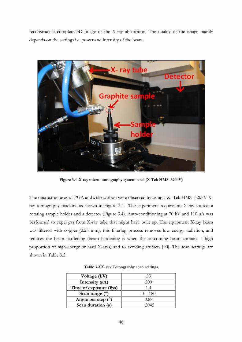
46
reconstruct a complete 3D image of the X-ray absorption. The quality of the image mainly
depends on the settings i.e. power and intensity of the beam.
Figure 3.4 X-ray micro- tomography system used (X-Tek HMS- 320kV)
The microstructures of PGA and Gilsocarbon were observed by using a X- Tek HMS- 320kV X-
ray tomography machine as shown in Figure 3.4. The experiment requires an X-ray source, a
rotating sample holder and a detector (Figure 3.4). Auto-conditioning at 70 kV and 110 µA was
performed to expel gas from X-ray tube that might have built up. The equipment X-ray beam
was filtered with copper (0.25 mm), this filtering process removes low energy radiation, and
reduces the beam hardening (beam hardening is when the outcoming beam contains a high
proportion of high-energy or hard X-rays) and to avoiding artifacts [90]. The scan settings are
shown in Table 3.2.
Table 3.2 X- ray Tomography scan settings
Voltage (kV) 55
Intensity (µA) 200
Time of exposure (fps) 1.4
Scan range (°) 0 – 180
Angle per step (°) 0.88
Scan duration (s) 2045

47
The sample is rotated by motorised turntable while scanning. The typical resolution accessible by
this equipment is 11.3- 14.6 µm per voxel
One thousand eight hundred radiographs of the sample were taken during each scan. The VG
studio package was used to reconstruct the volume of high-resolution images obtained. The
sample height used varied from 40 - 50.8 mm. Three-dimensional images of virgin PGA and
Gilsocarbon comprised 1900 x 1900 x 1800 voxels. A voxel is a volume element representing a
value in 3D space, and it can be coded in 8, 16 and 32 bits, but in this work it was coded in 8bits
with a grey scale of 0 - 256 (28 values). The high-resolution images obtained from this equipment
allow the characterisation of graphite microstructure such as porosity morphology.
3.2.2 X-ray texture goniometry
The preferential crystal orientation in the PGA and Gilsocarbon nuclear graphite prepared by
extrusion and moulding respectively were investigated. Young’s modulus of a polycrystalline
aggregate without porosity was calculated from the orientation distribution function (ODF). A
quantitative description of orientation characteristics gave a good interpretation of texture in a
given sample. The term ‘texture’ is a collective term for a non-uniform distribution of
crystallographic orientations in a polycrystalline aggregate or is a synonym for preferred
crystallographic orientation in the polycrystalline material [91]. Texture analysis is the
determination of the preferred orientation of the crystallites in polycrystalline aggregates. It is not
possible to measure directly the distribution of crystal orientations in a polycrystalline sample by
bulk diffraction techniques. Texture goniometry is only capable of determining the distribution
of crystal poles and further analysis is required to extract the orientation distribution from these
data. The preferred orientation is usually described in terms of pole figures [91, 92].
X- ray diffraction is a non-destructive analytical technique used for identification and qualitative
determination of the various crystalline forms or phases in a material. X-rays are generated by a
cathode ray tube, filtered to produce monochromatic radiation, collimated to concentrate, and
directed toward the graphite sample [25, 93]. The interaction of the incident rays with lattice
planes within the sample produces constructive interference and a diffracted ray when conditions
satisfy Bragg's law;
(3.1)

48
This law relates the wavelength (λ) of electromagnetic radiation to the diffraction angle and the
lattice spacing (d ) of the lattice plane that is causing the diffraction, n and θ are integer and
incident angle [93]. These diffracted X-rays are then detected and counted. By changing the
geometry of the incident rays, all possible diffraction conditions for each grain were explored. In
this work, Phillips X’pert 1 goniometry was used to scan the graphite samples.
Table 3.3 XRD scan settings
Angles Phi (Φ) Psi (ψ)
Scan range (°) 0 -360 0-85
Step size (°) 0.05 0.05
Time/step (s) 10 10
Scan duration (s) 72000 17000
Texture goniometry measures the intensity of the diffracted X-rays for a specific 2θ (e.g. for a
specific lattice plane) over a whole range of sample orientations. The sample orientation is
usually expressed in terms of 2 Euler angles phi (Φ) and psi (ψ). This data is then density
controlled and represented on a stereographic projection of a hemisphere (often called pole
figures) here different points on the hemisphere represent different orientations of the sample.
A texture scan used, three peaks ([002], [100], and [110] planes) selected randomly amongst the
other peaks for texture measurement, the scan settings are shown in Table 3. A texture
measurement is also referred to as a pole figure. In Figure 3.5, considering the plane (h, k, l) in a
given crystallite in a sample, the direction of the plane normal is projected onto the sphere
around the crystallite. The point where the plane normal intersects the sphere is defined by two
angles, a pole distance (ψ = 85o) and an azimuth (Φ= 360o). Occasionally and are used to
represent the pole distance and azimuth angles respectively. The azimuth angle is measured
counter clockwise from the point E (East). The intensity of a given reflection (h, k , l) is
proportional to the number of h, k, l planes in diffraction condition (Bragg’s law). Hence, the
pole figure gives the probability of finding a given crystal-plane-normal as function of the
specimen orientation. If the crystallites in the sample have a uniform distribution of orientations
recorded then intensity will be uniform [94]. Assuming that the plane normal for the plane (h, k,
l) are projected from all the crystallites irradiated in the sample onto the sphere, each plane
normal intercepting the sphere represents a point (X) on the sphere.

49
Figure 3.5 Schematic diagram of stereographic projection (sample orientation is usually expressed in terms of 2 Euler angles phi (Φ) and psi (ψ))
3.2.3 Pole figure
A pole figure is a projection of directions on to a plane. It is described when intensity
distribution gained from the measurement of a lattice reflection with indices (h, k, l) where the
sample is rotated around two axes (angles ψ and Φ) is drawn into a polar grid using contours
lines [91]. The diffracted intensity is proportional to the fraction of crystallites within the tested
volume oriented in a specific direction. Three angles are required to define the orientation of a
crystallite in relation to the sample axes, a set of Euler angles ( ) are commonly used for
the consecutive rotations around the z-axis, x-axis, and again z-axis [95]. The texture of a tested
sample can be also described completely by the orientation distribution function with the
orientation, ), this is described later in this chapter. A representation of the crystal
orientation with respect to a unique sample orientation is called an inverse pole figure. Any
sample orientation with respect to an external reference frame has its own inverse pole figure.
3.2.4 Intensity corrections and data reduction
A Complete pole figure cannot be measured by laboratory X-ray diffraction due to the strong
defocusing effect and diffraction geometry, therefore the obtained intensity need to be corrected.
Background corrections and defocusing measurements were performed, by removing the
background and correcting for the beam defocusing that occurs as the ψ angle increases. As a
result more accurate pole figures are produced [94]. Background intensity results from

50
incoherent scattering and fluorescence in the sample, from interaction of the beam with air
molecules, and from electronic noise. Air scattering can be reduced by setting the incoming
beam collimator and a receiving collimator close to the sample or by measuring in a vacuum.
Background can also be reduced by choosing a small window for the pulse height analyser,
because most of the background x-ray photons have a different wavelength. In practise one
cannot eliminate the background, but the background intensity can be subtracted from the
measured intensity [91]. The background correction curve is best determined empirically on a
sample with similar composition but few diffraction peaks by placing the detector on a
background region removed from any Bragg peak. The first step in data correction is to subtract
the background from the intensity curve.
If
is measured background at then the background
at is
(3.2)
The ratio as shown in the Equation 3.3 is the empirically determined background correction
curve
(3.3)
The shape of the irradiated area depends on the collimating system and the orientation of the
sample surface relative to the incident x-ray beam. Since the x-rays penetrate the sample up to
about 100- 200 , the covered volume is larger and the true geometry is more complicated. The
spread in area and the resulting distortion of the reflected signal causes defocusing x-rays. X-ray
texture measurements usually record peak intensities rather than integrated intensities, the
intensity decrease with tilt is severe, and therefore it is necessary to correct the intensity.
An empirical defocusing correction curve can be measured on a sample of the same material or a
material with similar 2θ peak positions and the same sample geometry but with no preferred
orientation. In this case, a Gilsocarbon sample was used for the defocusing scan to correct all the
other texture scans; because it was assumed that Gilsocarbon has no preferred orientation. The
correction depends on the alignment of the instrument, the shape and size of collimator and
receiving slit, and the diffraction angle 2θ. A corrected intensity is obtained from;

51
(3.4)
Where is the measured intensity from the texture sample, and is the intensity from the
random sample at the same value of , all these intensities must be corrected for background.
The correction curves obtained from Gilsocarbon (uniform orientation sample) were used as
standard and applied to correct PGA samples. It was necessary to ascertain the uniformity of
texture of the standard by measuring a pole figure and applying empirical corrections. This
should produce a uniform distribution. The result from the standard sample is shown in chapter
4.
In this work, the pole figure was scanned from the center (ψ = 00), out to about ψ = 850 using
Philips X’pert 1 goniometer (Figure 3.6).
Figure 3.6 Philips X’pert 1 goniometer
It allows automatic scanning of the pole figure on a true spiral by changing and ψ
simultaneously and continuously [96]. By collecting pole figure data for several (h k l), the

52
complete orientation distribution function (ODF) of the material can be determined. This was
achieved using Mtex (Matlab toolbox) [97]. MTex is an open- source Matlab toolbox for texture
analysis and modelling [98]. It comprises functions to import, analyse and visualize diffraction
pole figure data, to estimate an ODF, and compute texture characteristics.
Figure 3.7 Texture analysis procedure (data regeneration)
The texture analysis procedure shown in the Figure 3.7 and it is summarised as follows
The pole figure data including the background and defocussing data were collected for
the following lattice planes [002], [100], and [110], and were imported in the command
window of Matlab
The graphite is Hexagonal with the following lattice spacings (a= 2.465 Ǻ, c= 6.753 Ǻ,
and angles; α = 900, β = 900, γ = 1200 and is in the 6/mm Laue group.
The script (m-file) was generated and worked with in other to visualize and to represent
the pole figures.
3.2.5 Orientation Distribution Function (ODF)
Preferred orientation of the crystalline regions in polycrystalline samples may be investigated by
X-ray diffraction. The information concerning the preferred orientation of each Bragg plane
obtained can be examined [99]. These data may be summarised concisely by a series of pole
figure diagrams. A collection of pole figure diagrams for a sample implicitly contains general and
useful information called the distribution of orientations of the crystallographic unit cell.
Mathematical procedures have been developed for deducing this information in the form of
crystallite orientation distribution [95, 100-102]. Once the crystallite orientation distribution
function has been determined, it may be used to compute pole figures for unmeasured planes.
The crystallite Orientation Distribution Function (ODF) offers the most complete
representation which can be gained from a given set of pole figure data [95]. Bunge [95] and
Kocks et al. [91] defined ODF ( ) as
(3.5)

53
The volume of all crystallites in a sample is denoted by , it contains an orientation within an
orientation region , may be specified in a numerous ways (i.e. Euler angles ). is
the total sample volume. The volume fraction of orientations within a certain region of
orientation space is then
(3.6)
Where x denotes the entire orientation space and denotes the region around the texture
component of interest. In common practice, uniform density, is normally set to 1. This is
often called orientation density in multiples of a uniform distribution (m.u.d.). When the
orientations are represented by Euler angles, the infinitesimal volume element is
(3.7)
(3.8)
Where 𝚯, is the pole distance and Ψ is the Euler angle (azimuth in pole figure) and 𝜙 represent
the tilt angle in goniometer, is area element, whose magnitude depends on declination, these
are shown in the Figure 3.8. The volume of element is corrected by .

54
Figure 3.8 Symmetric definition of Euler angles as spherical coordinates for a vector on the surface of a unit sphere (adapted from [91])
3.3 Porosity measurement
Helium pycnometry was used to measure the percentage of connected pores (effective porosity)
of each sample before and after deformation, while mercury porosimetery was used to measure
the porosity volume, size and distribution of deformed and undeformed samples. The porosity
distribution in each sample was compared with each other to gain more understanding of the
effect of high pressure on porosity and the pore size distribution.
3.3.1 Helium pycnometer
The helium pycnometer was invented by Edward Y.H. Keng in 1967 [103]. It is a non-
destructive instrument that allows the measurement of the volume and hence true density of
solid sample. This is achieved by employing Boyle’s law to determine the true sample volume.
Boyle’s law is employed with helium as the gas to determine the solid volume of a sample. The
technique is rapid, and is valid on clean and dry samples. As the size of helium molecule is very
small, it can the penetrates even the smallest open pores. In this work, the DHP-100 Digital
Helium Porosimeter (Figure 3.9) was used to calculate the effective porosity percentage in each
graphite sample before and after loading. The results are discussed in Chapter 4.

55
Figure 3.9 Helium Porosimeter
The effective porosity of the sample was calculated by applying the following procedure; the
Boyle’s law states that for an ideal gas, the pressure exerted by a gas held at a constant
temperature varies inversely with the volume of the gas.
(3.9)
Where R is the universal gas constant, P is the pressure of the system; is the volume of the gas,
n is the number of moles and T is the temperature. The helium gas in the reference cell
isothermally expands into a sample cell. Thus the pressure-volume products are equal before and
after opening the core holder valve.

56
Figure 3.10 Schematic diagram of helium porosimeter apparatus adapted from [104]
(3.10)
After expansion, the resultant equilibrium pressure is measured. The helium porosimeter
apparatus is shown schematically in the Figure 3.10.
Calculating grain volume requires the knowledge of (reference pressure, gauge
pressure reading, reference volume and sample chamber volume). The gauge pressure reading
was obtained when the helium expands into the specimen chamber and it was assumed that
temperature (≈ 20 OC) is constant. The ≈ 7 bar, reading was taking to 0.001 bar. In solving the
equation of unknown volume, ;
(3.11)
Since the product of the initial pressure and volume of the helium in the system is equal to the
final pressure and volume of the helium in the system. Therefore, if a sample of unknown
volume is placed in the core holder, its grain volume can be calculated by rearranging Equation
(3.12)
(3.12)
(3.13)
Theoretical bulk volume ( ) is calculated by using the equation of the volume of cylinder

57
(3.14)
The effective porosity is defined as the ratio of pore volume ( ) to bulk volume ( ), and
in this work it is expressed as a percentage ( ), in equation form
The open porosity of Gilsocarbon and PGA samples were measured in a helium pycnometer
before and after deformation, and the closed porosity was calculated by using the equations
below
(3.25)
(3.16)
Where VT represents the theoretical volume while the VC represents the volume of the
crystallites. The total porosity volume is the overall closed pore volume ( ) and open pore
volume ( ).
3.3.2 Mercury porosimeter
Mercury porosimetry can be used to characterize pore size distribution ranging from 0.003µm to
950µm. Some of the useful sample characteristics obtained are the total porosity, open
(accessible) porosities, mean pore diameter and distributions of the pore size, a direct
comparison was made between the amount of effective porosity available to mercury and to
helium. The experimental method in mercury porosimetry involves filling up an evacuated
sample holder with mercury and then applying pressure to force the mercury pore spaces [104].
Both applied pressure and intruded volume are recorded and the data produced can be used to
calculate the sample characteristic mentioned above.
Mercury porosimetry uses the Washburn equation (Equation 3.17) to describe the intrusion of
mercury into a porous material as a function of pressure applied to the mercury [104-106].
Mercury is used because it is non-wetting and non-reactive for most solid surfaces. It also has a
contact angle (θ) of about 140° for most solids and it will not enter fine pores until sufficient
pressure is applied to force its entry into the pore[105].
(3.17)
Where P, the applied pressure, is in MPa and , the pore radius, is in micrometers. PoreMaster
60 shown in Figure 3.11 was used for the mercury porosimetry measurements. It generates

58
pressure up to 414 MPa for pore size analysis from over 950 µm to 0.0036 µm pore
diameter[107]. The evacuation setting was increased to 2 hours to allow proper evacuation of the
glass cell and to allow mercury settling in the sample steadily during low pressure measurement.
Figure 3.11 PoreMaster series adapted from Quantachrome limited
The mercury porosimeter can cause damage to graphite specimens above a critical pressure
range, which could make the porosimetry measurements misleading [106]. The results of
porosity measurements are treated carefully taking account of the limitations of the technique,
therefore good absolute, comparative values of porosities were obtained.
3.4 Dynamic Young’s modulus measurement
The traditional method for measuring the dynamic elastic constants has been to employ an
ultrasonic method in which the time of flight of an ultrasonic pulse along a specimen is
measured [108]. A high frequency electrical pulse is transmitted to a sender piezoelectric
transducer that creates an ultrasonic wave that passes through the sample and is received by the
receiver piezoelectric transducer and reconverted to an electric signal [108, 109]. Travel time for
the pulse through the specimen is measured. The use of both compressional and shear

59
transducers permits both compressional waves and shear waves to be observed so that both
compressional wave velocity (VL) and transverse wave velocity (VT) can be determined. The bulk
density of each sample is calculated from the ratio of weight (mass) to bulk volume of the
sample. The dynamic Young’s modulus (E) and shear modulus (G) of each sample before and
after loading was calculated from the velocity of longitudinal waves and shear ultrasonic waves
using the following equation [108, 110]
(3.18)
(
) (3.19)
(3.20)
The equations above shows the relationships between longitudinal and transverse wave velocities
with Young’s modulus and shear modulus.
3.5 Triaxial Deformation Apparatus (Big rig)
The big rig consists of a pressure vessel using synthetic oil as the confining medium into which a
piston is introduced to apply elevated axial loads to the specimen; the confining pressure and
axial load are independently controlled and measured. This rig was initially designed to study
meso-scale fracturing processes. The rig is called big rig because it can be used to deform
relatively large sample (25 mm diameter 55 mm long cylindrical samples) and it can be used at
pressures up to 300 MPa.
The big rig allows compression testing by superimposing a hydrostatic pressure and uniaxial
stress. The system can deform samples under axially symmetric shortening or axially symmetric
extension by using a servo-controlled axial loading system that lower or withdraws the piston to
produce the required deformation conditions. The picture and the cross section of the big rig is
shown in Figure 3.12. A pressure vessel is housed in a cylindrical shaped steel shield.

60
Figure 3.12 Big rig and Schematic of the whole big rig system
Confining pressure was applied using a compressed air-driven Haskel-type pump (SC Pump 600)
to pressurize the vessel up to 7 MPa. Further confining pressure (up to 300 MPa) was controlled
using a servo-controlled pressure regulator above 7 MPa. The confining fluid is Di-ethyl ester
called Reolube-DOS® (chemically inert, no health hazard in use). Confining pressure was
measured using a pressure transducer which was calibrated against a high accuracy solid front
29617 Heise pressure gauge. Confining pressure can be measured to an accuracy of 0.156 MPa,
as shown in Figure 3.16.
3.5.1 Axial loading system
The axial loading system consists of ball screw press with an axial load capacity of 35tons. The
ball screw is driven via a short gear train; in turn driven by a DC servo motor with a maximum
speed of 3000 rpm and torque 90 Nm when driven by 60 Vdc from a servo- amplifier. The
servo-control system generates uniform axial displacement rate by measuring the displacement of
the piston with a LVDT (Linear Variable Differential Transformer) and automatically adjusting
the motor speed to keep the piston displacement rate constant. Axial displacement rates of 1.22
mm/min that correspond to strain rate of 0.0004 s-1 were used in this work for both small and
large samples respectively. The internal force gauge in the big rig measures axial force during the
axial deformation experiment. As the force deforms strain gauges, the strain gauges convert the
deformation strain to electrical signals and hence into a force value that is displayed on the
instrument. The force gauge was calibrated, the result is discussed below.

61
3.6 Pressure vessel (Seismic velocity rig)
This is a high pressure (500 MPa) rig designed for measuring seismic velocities of solid materials
at room temperature. Each sample was assembled (as shown in Figure 3.14) and placed in a
pressure vessel so that pressure can be applied. Acoustic velocity measurements were taken
during hydrostatic loading in the seismic velocity rig shown in Figure 3.13. In this experiment,
the acoustic transducers used are 25mm diameter piezoelectric ceramic plates supplied by
Morgan Acoustic Ceramics. The piezoelectric material used is lead zirconium titanate, referred to
as PZT (Pb(Zr,Ti)O3). These transducer plates (Sender and receiver) are operated when
confining pressure was applied; good acoustic and electrical connections are necessary to achieve
a good result. This work was carried out at confining pressure up to 200 MPa. The sample
lengths were measured before and after test, length corrections were considered during data
processing to take account of the change in volume and hence length of the sample due to the
applied hydrostatic pressure. The changes in axial and volumetric strain as graphite compressed
under hydrostatic compression are known from the static loading tests in the big rig. The results
obtained from this experiment allowed detailed comparison between volume change and velocity
change. The sample’s density was corrected in order to calculate the dynamic elastic moduli as
the sample compressed hydrostatically.

62
Figure 3.13 Picture and Schematic diagram of seismic velocity rig
Figure 3.14 Piston assembly

63
3.7 Strain gauge instrumentation
A strain gauge is a device used to measure the strain (axial and circumferential) of a solid material
by producing a resistance change proportional to the change in strain. YFLA-5-NOL post yield
strain gauges were used in this work; they were made and supplied by Tokyo Sokki Kenkyujo
Co. This gauge was used because it was designed for measurement of large strains up to 15 – 20
% without creeping or cracking. The gauge length, width and resistance are 5 mm, 2 mm and 120
± 0.3 respectively, with a gauge factor of 2.10 ± 2 %. The operational temperature is -20~+80
OC. CN-E glue is designed for bonding strain gauges to porous materials; the curing time under
normal conditions is 4 - 120 seconds. It was used to attach the strain gauges to the graphite
sample with the help of a technician (Bill Storey).
3.7.1 Sample assembly
Four strain gauges were attached to each sample, two strain gauges were attached parallel to the
sample axis and two parallel to the sample circumference. There are two layers of heat shrink
sleeving applied, one to protect strain gauges and connecting wires and the second to isolate the
sample from the confining pressure. The sample was jacketed with heat shrink to prevent the
wire attached to strain gauges from breaking. The strain gauge driving voltage is 125 ΩH. To
avoid heating, the energy generated by each gauge is 1 watt (YFLA-5-NOL post yield strain
gauges are sensitive to keeping low watt).
The sample was jacketed with heat shrink to the loading pistons. The connected cables were
pushed through the hole in the middle of the piston as shown in Figures 3.15A and 35B below
(final assembling). The whole assembly is lowered into the pressure vessel, making sure that it
was carefully placed on top of the internal load cell. The loading frame (gear train, ball screw,
driver motor and external loading cell) are pivoted into place and the main closure nuts are
tightened to the pressure vessel. The data logging proceeds for the duration of the test, the
output data is saved as text file containing raw data such as time (hours), time (seconds), strain 1,
strain 2, strain 3, strain 4, force (kN), volumetric strain, confining pressure (MPa). The saved files
can be opened in an Excel spreadsheet for further analysis. The sample final assembling is shown
in Figures 3.15A – 3.15D.

64
Figure 3.15 Sample assembling; A) component built by the author to protect the cables during pressurization, B) sample with strain gauges attached, covered with heat shrink, C) the sample jacketed to
the loading piston, D) the sample was jacketed with heat shrink to the loading pistons
3.8 Hydrostatic tests
Each cylindrical graphite specimen was subjected to confining pressure up to 30000 Psi (200
MPa). The pressure rate was controlled by a servo-controlled motor that moved a piston in and
out of a pressure vessel via a gear box and screw jack. Servo control was achieved with a
Eurotherm PID control which used the pressure transducer as the feedback. The longitudinal
and circumferential strains and pressure were continuously logged throughout the experiment.
When a pressure of 200 MPa was reached, the pressure was lowered at the same rate at which it
was applied and the strain was measured as the pressure was lowered. The loading and unloading
pressure-strain curves from the data points represent the deformation behaviour of graphite
under a complete pressure cycle. The effect of hydrostatic cycling on graphite deformation was
also investigated by repeating the whole hydrostatic test procedure. The effect of creep on

65
hydrostatic deformation was investigated by loading graphite up to 200 MPa and then holding
the pressure constant for 24 hours before unloading to atmospheric pressure.
3.9 Axial deformation tests
Axial compression was performed on hydrostatically compressed graphite specimens to obtain
useful data such as Young’s modulus and Poisson’s ratio. When the required confining pressure
(200 MPa) was attained, the axial drive motor was controlled automatically at desired
displacement rate (1.22 mm/min). Each sample was loaded to different stresses; cyclic axial
deformation test were also conducted to various differential stresses. At the end of the test, the
axial load was removed. The confining pressure was then released, and the sample was taken out
of the rig.
3.10 Seismic velocity measurements
The compressional and shear wave velocities were determined for the samples from the transit
time of ultrasonic pulses (approximately 1 MHz). The time difference between the two
transducers (sender and receiver) is the time required for the group stress waves to travel
through the specimen. The higher the excitation frequency, the more reliable is the time pick
(sharp first break at the receiver), but more attenuation occurs at higher frequencies, both within
the sample and through the decrease in gain of the pulse amplifier with frequency.
A signal generator (TG130S Oscillator) was used to generate 1 V peak to peak (P - P) square
wave pulse or half cycle sinewave. This pulse was amplified to provide a driver waveform of up
to 150 V- 400 V P-P for piezo transducer (sender). The rise of the driver waveform was used to
trigger a LeCroy 300 MHz digital storage oscilloscope. The detected signal from the piezo
transducer (receiver) was connected to the LeCroy9310 Oscilloscope. The signals (pulses at
300ms interval) were averaged to reduce noise. Time of flight was read off from the oscilloscope
trace to a resolution of 0.0075 s. In choosing the first break, it is estimated that the time could
be estimated reliably to half of 1 % of the time of flight. The time of flight through the steel
piston at each end of the specimen (determined separately) was subtracted from the total time of
flight through steel and sample. This was conducted by measuring the time delay with the platens
in contact (no sample) with an applied load.

66
3.11 Calibration data (Hydrostatic pressure measurement)
The big rig loading system was calibrated by carrying out hydrostatic and axial deformation tests
on an EN24 steel specimen in order to measure the strain in a material with well-known elastic
properties. Confining pressure was measured using a pressure transducer with an excitation
voltage of 11.72 V. The calibration was carried out, and was very linear with parameters 47.1
MPa/mV with 0.16 mV output at zero pressure. The calibration graph of the pressure
transducers and the force gauge are shown in the Figures 3.16 and 3.17 respectively. At zero
force, the internal force gauge output during loading and unloading are 0.0782 V and 0.1641 V
respectively.

67
Figure 3.16 Calibration for the pressure transducer, the voltage supply is 11.72V
Figure 3.17 Big rig force gauge calibration

68
3.12 Calibration data (Hydrostatic P- and S- waves measurements)
The total time of flight of the ultrasonic pulse recorded includes the time taken for the wave to
travel through the steel piston between the piezoelectric transducers and the sample. A
correction for this time must be made. This was achieved through running a calibration with no
sample so that the pistons are in direct contact with each other, so that the time of flight
measured is only the time taken for the seismic wave to pass through the pistons. Such a
calibration was run at a number of pressures and the pressure of flight was seen to decrease with
time for two reasons
the steel was becoming slightly stiffer with increasing pressure and
the length of the steel piston reduced as the pressure increased.
Such a calibration is shown in the Figure 3.18.
Figure 3.18 P-P transducer Assembly Calibration
The linear equations obtained from the pressure circle in Figure 3.18 were used to correct the
time of flight of the P-waves on all the samples measured. Dynamic Young’s modulus and shear
modulus were calculated from the P- and S- wave velocities respectively using Equations 3.18
and 3.20 in Chapter 3.

69
The P-S sample- transducer arrangement allows simultaneous measurements of P and S
velocities. The P-S sample was loaded up to 208 MPa without a sample and the history of
pressure versus time of flight is shown in Figure 3.19.
Figure 3.19 P-S transducer Assembly Calibration
Similar calibration that was done with the P-P transducer assembly in the Figure 3.18 was
repeated with the P-S transducer assembly, the calibration is shown in the Figure 3.19. The linear
equations obtained from the pressure circle in the Figure 3.19 were used to correct the time of
flight of the S-waves on all the samples measured in this experiment. Shear moduli was
calculated from the S- wave velocities respectively using Equation 3.20 in Chapter 3
3.13 Conclusion
The mechanical properties of nuclear graphite are necessary to determine the structural integrity
of graphite component in a reactor. These mechanical properties (static and dynamic elastic
moduli, uniaxial strength, strain to failure e.t.c.) are vital to determining the capability of the
structural strength and integrity of the reactor core.

70
The irradiation changes to graphite properties are related to opening and closure of porosity and
reorientation of the crystallites in polycrystalline graphite. Loading graphite under high
hydrostatic pressure (up to 200 MPa) is a method of simulating this behaviour and was employed
in this work. In order to understand changes in graphite microstructure under stress, a change in
microstructure will be induced by loading the samples hydrostatically and also with differential
stress, using two high pressure rigs (big rig and seismic rig).
Non-destructive X-ray tomography will be investigated for its ability to determine the
microstructure within individual test samples. It allowed samples to be analysed before and after
the loading tests. Image analysis techniques (using Matlab) will be used to enhance information
such as pore size distribution in the virgin and deformed micrographs. The visible
microstructural change in the deformed sample micrographs due to stress history will be
compared to the original micrographs, so that the microstructural evolution and modifications as
a result of hydrostatic stress can be established. The X-ray diffraction method will be
investigated in order to examine the orientation of the crystals in the graphite microstructure
before and after tests.
Precise dimensional measurements (diameter and length) of all deformed samples will allow
macroscopic dimensional changes to be determined; the pore size distribution of the deformed
samples will be calculated (using helium and mercury porosimeter) and compared to virgin
samples values for each test. Each cylindrical shaped graphite sample’s identity (ID), the
dimensions and the samples direction of extrusion (AG and WG) is shown in the Table 3.4.

71
Table 3.4 The samples identities, directions and dimensions as well as the test done on each sample
Sample ID Direction Diameter
(mm)
Height
(mm) Machining and Experiments
Gilsocarbon A2 9.97 20.03 Machined to 9X19 mm cylindrical shape samples for Hg porosimeter
E1 20.02 40.04 It was loaded up to 200 MPa in seismic rig, but there was a leak
E2 20.02 40.04 Confining pressure of 200 MPa
E3 20.02 40.04
E4 20.02 40.07 Machined to two 9X19 mm cylindrical shape samples for Hg porosimeter
I1 24.96 50.84 Confining pressure of 200 MPa
I2 24.98 50.84 Confining pressure of 200 MPa and cyclic differential forces of 28 KN & 17 KN
I3 24.98 50.85 Confining pressure of 202 MPa and cyclic differential forces of 36 KN & 20 KN
I4 25.37 50.81 Seismic loading up to 207 MPa with a P rod (Pwave)
I5 25.37 50.81 Seismic loading up to 207 MPa with a S rod (P&Swave)
I6 25.37 50.81 Seismic loading up to 207 MPa with a S rod (Swave)
I7 25.34 50.81 Cable disconnected twice during the test, sample was still loaded up to 80 MPa
I8 25.37 50.82 Cyclic confining pressure of up to 200 MPa, down to 20 MPa, up to 200 MPa,down to
16 MPa, up to 100 MPa
I9 25.37 50.82
I10 25.38 50.82 Cyclic seismic loading up to 207 MPa with a P rod (Pwave)
I11 25.38 50.82 Machined to two 9X19 mm cylindrical shape samples for Hg porosimeter
PGA B2 WG 9.97 20.02 Machined to 9X19 mm cylindrical shape samples for Hg porosimeter
B4 AG 10 20.04 Machined to 9X19 mm cylindrical shape samples for Hg porosimeter
F1 WG 20.02 40.06 Confining pressure of 200 MPa
F2 WG 20.01 40.15 Confining pressure of 60 MPa and cyclic differential forces of 16 KN & 11 KN
F3 WG 20.03 40.07 Confining pressure of 60 MPa and cyclic differential forces of 17 KN & 12 KN

72
F4 AG 20.02 40.07 Confining pressure of 60 MPa
F5 AG 20.03 40.07 Confining pressure of 200 MPa
F6 AG 20.02 40.04 Repetition of J8 but Confining pressure of 200 MPa and cyclic differential forces of 17
KN & 20 KN
F7 AG 20.04 40.09 Confining pressure of 60 MPa and cyclic differential forces of 16 KN & 11 KN
J1 WG 25.01 50.85 Confined up to 58 MPa, then shut circuit, sample reassembled and loaded up to 200
MPa
J2 WG 25.01 50.88 Confining pressure of 200 MPa and differential force of 28 KN
J3 WG 25.01 50.84 Confining pressure of 200 MPa and cyclic differential force of 17,20,23 & 28 KN
J4 WG 25.01 50.99 Confining pressure of 60 MPa
J5 AG 24.99 50.85 Confining pressure of 120 MPa
J6 AG 25 50.87 Shut circuited during test, beside the sample cracked, therefore the result was not
reliable
J7 AG 24.98 50.84 Confining pressure of 200 MPa and differential force of 28 KN
J8 AG 24.97 50.84 Confining pressure of 200 MPa and differential force of 36 KN
J9 AG 25.35 50.84 Seismic loading up to 207 MPa with a P rod (Pwave)
J10 AG 25.37 50.84
J11 AG 25.38 50.81
J12 AG 25.32 50.81 Cyclic confining pressure of up to 200 MPa, down to 20 MPa, loaded and unloaded at
200 MPa
J13 AG 25.31 50.82 Machined to 20X39 mm cylindrical shape sample for Hg porosimeter
J14 AG 25.36 50.82
J15 AG 35.35 50.82 Seismic loading up to 207 MPa with a S rod (Swave)
J16 AG 25.36 50.82
J17 AG 25.36 50.82
J18 AG 25.34 50.82 Machined a disk for XRD experiment & 9X19 mm cylindrical shaped sample for Hg
porosimeter
J19 AG 25.36 50.82

73
J20 AG 25.33 50.82
J21 WG 25.33 50.73
J22 WG 25.28 50.72 Confining pressure of 200 MPa, loaded and leave up to 24hours before unloading (creep
test)
J23 WG 25.31 50.73 Cyclic seismic loading up to 207 MPa with a P rod (Pwave)
J24 WG 25.31 50.73 Seismic loading up to 207 MPa with a S rod (P&Swave)
J25 WG 25.3 50.73 Machined to 20X39 mm cylindrical shape sample for Hg porosimeter

74
CHAPTER 4
4 Results
The irradiation changes to bulk properties are said to be, in part, related to closure of porosity
and reorientation of the crystallites [60, 82]. Pore closure and crystallite reorientation can be
mimicked by loading graphite under high hydrostatic pressure [54]. PGA (WG and AG) and
Gilsocarbon nuclear graphites were loaded hydrostatically up to 200MPa, the relationships
between the graphites’ mechanical properties such as static and dynamic bulk modulus, shear
modulus and Poisson’s ratio were analysed. The relationships between the mechanical properties
of different loading modes such as
hydrostatic loading using strain gauges,
hydrostatic loading followed by shortening,
cyclic hydrostatic loading,
measuring acoustic loading under hydrostatic stress to express the moduli
were analysed. This research combined measurement of properties under high pressure and
compares the experimental results with various to effective medium (EM) models in Chapter 5.
Each sample was characterized before (pre-microstructural characterization) and after loading
(post-microstructural characterization), by using the equipment listed in the Chapter 3. The
results obtained are discussed in this chapter.
4.1 Pre-microstructural characterization and properties measurement
4.1.1 X-ray goniometry results
A summary of the experimental X-ray diffraction spectrum is shown in Figure 4.1, showing the
positions of all Bragg reflections. A general texture two dimensional scan was taken; three peaks
were needed for the texture measurement. Several pole figures are needed to define the ODF (as
discussed in the Chapter 3). Since the 002, 100 and 110 peaks are the most intense and sharp
peaks, they were selected for the texture measurements.

75
Figure 4.1 X-ray diffraction spectrum for PGA
The pole figures shown below (Figures 4.2 and 4.3) are only projections of three crystallographic
axes of the full ODF. The pole figures describe the orientation distribution of all crystal cells of a
given phase of the sample. The experimental pole figures of the sample for three graphite crystal
planes (h k l) are determined by X-ray diffraction and they are shown in the Figures 4.2a and
4.3a. Gilsocarbon (Figure 4.2) is nearly isotropic, this is shown by uniform intensity across the
pole figures while PGA (Figure 4.3) showed preferred orientation (anisotropic characteristic).

76
Figure 4.2 Pole figures of the considered Gilsocarbon graphite sample, a) experimental figures derived by the X-ray diffraction method, b) recalculated pole figures from ODF derived from the experimental pole
figures, c) difference between calculated ODF and the experimental data. The set colour range in represent the intensity scales. The colour range have no unit, it was denoted as multiples of uniform
distribution (mud) values. It varies from 0 to 1.2mud for the ODF derived
The region of extreme intensity is in some way correlated with the axes of the sample coordinate
system (X is the extrusion direction; Y and Z are approximately parallel to the other sides of the
original graphite block). The calculated pole figures in the Figure 4.2b show no preferred
orientation (the grains are uniformly orientated), however there is an artifact around the
circumference. The original pole figure data collected below 75O tilt of the sample can be trusted;
the data above 75O is unreliable because of defocusing of x-ray beam which in systematically
lower intensity as the tilt is increased. The pole figures for PGA were corrected for the
defocusing effect using pole figures for a sample of Gilsocarbon, that has almost no lattice
preferred orientation. The moulding of Gilsocarbon might have led to the random orientation of
the graphite crystal cells in the block, and having spherical grains (Gilsocarbon coke) or grains

77
within which the layer plane orientation which has considerable variation, these contributed to
the isotropic nature in Gilsocarbon [111].
Figure 4.3 Pole figures of the considered PGA (against grain) graphite sample, a) correction of the experimental figures derived by X-ray diffraction data, b) recalculated pole figures from ODF derived from
the experimental pole figures, c) difference between calculated ODF and the corrected x-ray data, d) Young’s modulus calculated from elastic tensor of a single crystal and ODF. The colour range varies from
0 to 1.7 mud for the ODF derived.
It can be seen that PGA has a preferred orientation of the lattice planes especially the basal
planes (Figure 4.3). This is in contrast to Gilsocarbon which has a more random distribution
(Figure 4.2). The lattice preferred orientation LPO of anisotropic PGA graphite can be seen
from pole figures where the (0001) poles and hence c-axes are preferentially oriented in a plane
perpendicular to the extrusion direction. There are weak clusters of the ( ̅0) and ( ̅0) axes
parallel to the extrusion (Figure 4.3).

78
It is possible to calculate the bulk properties of a polycrystalline material if the properties of the
single crystal and ODF are known [112]. The Young’s modulus in different directions can be
calculated from the single-crystalline graphite elastic tensor(Cij) [21] and ODF assuming the
aggregate has no porosity. The minimum and maximum Young’s modulus of PGA calculated in
this way are 283 GPa and 330 GPa respectively (Figure 4.3d), these clearly indicated that the
modulus is higher in the direction (x) parallel to the extrusion direction than in the plane
perpendicular to the extrusion direction. These Young’s moduli calculated are 28 - 32 times
stiffer than the modulus of polycrystalline nuclear graphites (Gilsocarbon and PGA). This is due
to the present of 18-26 % porosity in the polycrystalline graphites.
The graphite elastic tensor obtained from Bosak [21] was used to calculate the VRH elastic bulk
modulus by using Berryman’s equation [113]. The effective bulk moduli of non-porous graphite
calculated is 36 GPa. The effect of porosity on Bulk modulus was considered by using models
such as VRH, HT and KT. The effective bulk modulus (36 GPa) was used and addition of
porosity was also considered in the models. This is discussed later in Chapter 5.
4.1.2 Tomography scans and mercury pycnometry results
The virgin PGA and Gilsocarbon microstructural properties and porosity distributions were
characterised using X-ray computed tomography, helium pycnometry and mercury porosimetry.
Example tomographic images of PGA and Gilsocarbon are shown in the Figure 4.4. The grey
region (region that absorbed X-rays) in the tomographic image represents the graphite material
whilst the black region (region with no X-rays absorption) represents the porosity.

79
Figure 4.4 Tomography of Virgin PGA and Virgin Gilsocarbon (Gilso)
This non-destructive method allows investigation of the microstructural changes before and after
deformation. The smallest resolvable feature in the tomographic image is 14.6 , and the
change in microstructural features below this resolution was not visible. Since graphite
microcracks closure and formation have also been reported in previous work [54] to be
responsible for changes in elastic properties, it was important to investigate porosity size ranges
beyond the resolution of the tomography technique. Therefore the changes in microstructure
were analysed by using mercury porosimetry and helium pycnometry to measure the porosity
distribution and total porosity in the virgin and deformed graphite. According to previous
work[4], the pore entrance radius in nuclear graphite ranged from nanometres to micrometres
(100 ). In this work, the pore entrance radius ranged between 3.6 to 100 as shown in
the Figure 4.5.

80
Figure 4.5 Normalised PGA open pore volume entrance radius versus open pore volume
The mercury porosimetry of different sizes of PGA samples (J18 and J25) are compared with
other data for PGA [4, 114]. The pore volume of each PGA graphite is normalized by its
maximum value in order to compare the author’s data to previous work (as shown in Figure 4.5).
Sample J25 was a large virgin PGA sample (20 mm diameter by 39 mm in length). Therefore the
pore distribution analysis was carried in a macro cell assembly (27 mm diameter by 40.6 mm in
length) attached to the porosimeter kit. The pore radius measurement showed an inconsistency
between the low pressure and high pressure measurements, which suggested that there was
insufficient mercury available to fill the pores of such a large sample.
Sample J18 was a small virgin PGA sample (9 mm diameter by 19 mm in length). Therefore the
pore distribution analysis was carried in a small cell assembly (11 mm diameter by 25 mm in
length) attached to the porosimeter kit. The pore radius measurement showed consistency
between the low pressure and high pressure measurements, which suggested that there was

81
sufficient mercury available for the analysis due to the smaller size of the sample compared with
sample J25.
Fazluddin [84] porosity distribution was similar to the author’s measurements (J18) at high
pressure as well as Williams’ [114] data. At low pressure, the data in the work of Fazluddin [84]
increased sharply suggesting that the low pressure measurement might have been run faster due
to scan mode settings and short evacuation period compared with the 2 hours evacuation
settings used in this study.
Figure 4.6 Pore size distribution in Virgin PGA (B2, B4 and J18) and Gilsocarbon (A2, I11 and I11b) nuclear graphite
Both PGA and Gilsocarbon samples showed a distribution within the macropore region
extending to the mesopore and micropore regions as shown in Figure 4.6. At higher pressures

82
(13.8 - 20.6 MPa- critical pressure range) measurement, porosity is being created by injected
mercury opening new cracks. Previous work [4, 114] suggested that some closed porosity was
graphites was made accessible under high mercury pressure and also completely new porosity are
generated. The additional accessible porosity might be caused by mechanical break-down of thin
pore walls and the rest by reversible elastic crack opening. Therefore it was safer to use mercury
porosimetry data only below a critical porosimetry pressure. The critical pressure was estimated
from the porosity curves in Figure 4.6. PGA’s open pores cumulative mercury intruded volume
was 0.225 cm3 (red line) while the Gilsocarbon open pores cumulative mercury intruded volume
was 0.1125 cm3 (blue line), these values of open pore volume are roughly coincident with an
inflexion point in the maximum value of open porosity obtained from the helium pycnometry
results. According to previous work [106], the critical porosimetry pressure for most graphite lies
between 13.8 - 20.6 MPa. In this work, the mercury porosity was equal to the helium porosity at
an intermediate pressure of 20.6 MPa, corresponding to a pore radius of about 0.05 µm.
The PGA graphite samples had the largest volume of open porosity volume due to high
cumulative volume of mercury intruded (0.225 cm3) compared with Gilsocarbon samples which
had a lower mercury intrusion volume (0.113 cm3). The volumes of mercury intruded into PGA
and Gilsocarbon were similar to the average open porosity (22% and 10% respectively) obtained
from helium porosimetry. It can be physically observed that the graphite microstructure has a
wide range of small pore sizes, with a fair proportion of large pores, but the pores size
distribution does reflect this. The Graphite material is heterogeneous; therefore different parts of
the graphite machined from the same graphite block could show similar or different porosity
distribution from each other as shown in the Figure 4.6. After measuring the open porosity by
helium pycnometry, the calculated closed porosity of the PGA and Gilsocarbon samples were
4% and 8% closed porosity respectively.
4.1.3 Dynamic Young’s modulus and helium pycnometer results
Dynamic moduli (Young’s modulus and shear modulus) were measured before and after
deformation by using bench top piezoelectric transducers at atmospheric pressure. The
Gilsocarbon microstructure is near isotopic and therefore can be an elastically isotropic linear
material which can have their elastic properties determined by any two of the following moduli;
Young’s modulus (E), Poisson’s ratio (υ), Bulk modulus (K), Shear modulus (G), and P-wave
modulus(M). From any two moduli, any other elastic moduli can be calculated. Bulk modulus is
calculated by using Equation 4.1 below

83
Due to graphite spatial heterogeneity, each graphite sample from the same graphite block can be
expected to display significant differences in moduli as shown in the Figures 4.7 and 4.8.
Table 4.1 Average DYM of the graphite
Graphite Average E (GPa) Average G (GPa)
PGA-WG 11.1 4.2
PGA-AG 5.9 3.3
Gilsocarbon 12.4 5.1
The average DYM and shear modulus of PGA-WG, PGA-AG and Gilsocarbon were shown in
the Figures 4.7 and 4.8. These values (shown in Table 4.1) correspond with the values from
previous work [115, 116] on PGA (DYM = 11.7 GPa and shear modulus = 5.4 GPa
respectively) and Gilsocarbon (DYM = 11.6 GPa). There was a vague trend of DYM lowering
with increase in porosity in the PGA while the Gilsocarbon DYM seemed to be independent of
porosity.
Figure 4.7 Dynamic Young’s modulus (DYM) against total porosity in PGA-WG (PGA sample parallel to the extrusion direction), PGA-AG (PGA sample against the extrusion direction) and Gilsocarbon

84
Figure 4.8 Shear modulus against total porosity in PGA-WG (PGA sample parallel to the extrusion direction), PGA-AG (PGA sample against the extrusion direction) and Gilsocarbon
4.2 High pressure loading (hydrostatic measurement)
Variation of volumetric strain of PGA-WG with hydrostatic pressure up to 60 MPa and 200
MPa are depicted in Figure 4.9. The conventional stress-strain curve for graphite aggregates
under uniaxial stress have a convex upward shape [42, 56], and it is interesting that observe the
resulting curve from hydrostatic compression exhibited a concave shape. The generic behaviour
of the graphite aggregates under hydrostatic stress is divided into three stages: these can be
marked I, II and III on the volumetric strain curve for the 200 MPa experiment in the Figure 4.9.
The stages were described in the Table 4.2

85
Figure 4.9 Volumetric strain (V.S.) of PGA-WG- J4 and F1 during hydrostatic compression up to 60MPa (dotted line) and 200MPa (solid line). The volumetric strain was changed from negative strain to positive
strain. The three stages (I, II and III) were explained in Table 4.2
When a sample is compressed, the change in length and strain are negative, but for the purpose
of clarity in this work, the negative strain was changed to positive strain. In the Figure 4.9, the
samples J4 and F1 were compressed, the sample sizes were reduced as the confining pressure
increased. The removal of applied pressure results in a small amount of permanent strain
indicating that there are some pores must have collapsed permanently during initial loading.
There was a remarkable volume recovery during the release of confining pressure at ~50 MPa;
for the PGA sample compressed at 60 MPa, original volume was approximately recovered, but
for the sample compressed at 200MPa, 98-99% volume recovery was noted. A permanent set of
1 - 2 % was comparable with Paterson’s work [54]. The postulated mechanisms for the graphite
inelastic and recovery behaviour are presented in Table 4.2.

86
Table 4.2 Description of graphite inelastic and recovery behaviour using the volumetric strain curve
Stages Loading Unloading
I
The strain increased with an increasing
in pressure (up to 8 %). It is suggested
that there might be not enough
pressure to overcome the friction
between the basal plane, lower rate of
pore closure with increase in pressure
Rapid volume recovery at below 50 MPa was
observed. This behaviour was generic to both
PGA with-grain and against-grain. It is
suggested that during this stage there was
enough pressure release to overcome the
friction between the basal plane
II
The strain increased substantially with
small increase in pressure (from 8-21
%). The author suggests that the
graphite deforms and large pores close
easily (i.e. lenticular and globular
porosity)
From 150 to 50MPa, the material slightly
recovered 1% of its volume after loading.
III
The strain almost level off with the
pressure (from 21-22 %). According to
Yoda et al. [56], this behaviour can only
be observed in elastomer material e.g.
rubber.
Majority of graphite pores closed at
high pressures (approaching zero
porosity); therefore for further increase
in pressure makes the graphite less
deformable and grain compression
dominate. The graphite behaviour
approaches hypothetically non-porous
graphite.
Many pores disappeared; the material held on
to its strain (22 %), even though the
confining pressure was released, the material
volume remains constant.
The behaviour of graphite under hydrostatic loading can also be explained further by using
micromechanical model such as spring and frictional element diagram shown in the Figure 4.10,
where Ka and Kc represent the two springs and F represents the frictional element (Ka ~ Kc ) and
(Kb « Ka ).

87
Figure 4.10 Spring/frictional element diagram
Considering the loading behaviour of graphite samples (i.e. sample F1 in the Figure 4.9), it was
initially stiff then it became less stiff after a few percent volume strain and then after about 20%
the material stiffens up again.
Conceptually it was envisaged that during the initial loading, the graphite was initially stiff as
large, equant pores are not closing. In the model above the initial loading represent compression
of spring Ka. Once some critical value of stress is reached, to overcome either friction on basal
planes or break some van der Waal’s bonds between basal planes, then the frictional element (F)
will slide, the spring Kb hit the buffer (combination of Ka and Kb), allowing the less-stiff Kc to be
loaded which represents the poroelasticity of the smaller inequant cracks and pores. Once all the
large pores have closed (represented by the limited displacement capacity of Kc), Kc will no
longer be able to accommodate any strain therefore any further strain will have to be
accommodated by further displacements on the stiffer Ka which represents the elasticity of the
graphite with remaining open microcracks and the collapse of the more equant larger pores.
During unloading, the slope of the stress/strain curve was steep and in the model above, the
spring Ka was been unloaded without sliding on the frictional element and Kc does not unload.
Once the stress difference on either side of the frictional element had reached a critical value, it
started to slide unloading Kb and finally unloading Kc. One possibility of explaining this is when
the equant porosity closes, basal planes of graphite are placed together and they bind together
with weak van der Waals bonds. They only break on release of the pressure when there is critical
stress on them. One of the ideas for interpreting the hysteresis was to see whether this was
possible with the energy lost in the process.
Mechanical workdone is the area under stress-strain curve. Work was done on the sample as it
was compressed. This energy was stored as strain energy. Since the material showed hysteresis
behaviour during unloading, only some of this energy was recovered. In the Figure 4.11, the

88
energy lost during loading and unloading was calculated as ~155 J. This energy must have been
dissipated through:
creation of new surface area by rupture and sliding of the basal planes (i.e. crystallites
reorientation resulting to porosity closure and opening) as suggested by Abrahamson
[117]
dissipation through plastic deformation and defect creation (creation of basal plane
dislocations)
heat lost ( : the heat lost was calculated (using thermodynamic equation; )
to be ~308.2 K/35 OC
Figure 4.11 Energy lost in the stress- strain curve of sample F1
The work done per unit volume to deform a material from a stress free reference state to a
loaded state is the strain energy density of that material. The strain energy density was calculated
as 12.3 MJm-3. In this work, the effect of the loading on the graphite microstructure was
examined.
PGA-WG and PGA-AG samples were hydrostatically compressed up to 60 MPa in order to
study the effect of graphite crystallite orientation on their compressibility. PGA-WG axial strain

89
was less than circumferential strain as shown in the Figure 4.12, but PGA-AG showed opposite
behaviour. This behaviour was due to the preferential alignment of the graphite grains in
different direction (i.e. PGA-WG: parallel to extrusion direction, therefore it became easier to
close the pores perpendicular to the circumferential strain gauge, whilst vice-versa for PGA-AG).
The volumetric strain is independent of the alignment of the specimen. The PGA-AG was taken
to higher pressure than PGA-WG, therefore the volumetric strain of PGA-AG is larger than
PGA-WG. In Figure 4.12, the true error was calculated using error propagation between extreme
individual observations in strain was represented with the error bars, this serves as a form of
reliability of the observed strain. The uncertainty in the confining pressure was calculated as ±
150 - 155 Pa, which was too small to be included in Figure 4.12.
Figure 4.12 The history of axial, circumferential and volumetric strain during hydrostatic compression of PGA with grain-J4 (dotted line) and PGA against grain-F4 (solid line) at 60 MPa. A.A- Average axial strain,
A.C- Average Circumferential strain, V.S- Volumetric strain
The schematic diagram in the Figure 4.13 was proposed in order to interpret the result in the
Figure 4.14 in term of porosity closure. The two dimensional schematic diagram in the Figure
4.13 shows the alignment of elliptical pores (i.e. lenticular cracks) parallel to the basal plane and
other randomly oriented circular porosity (i.e. globular pores) in the binder. Polycrystalline
graphite consists of binder, grains and porosity [23, 25, 41, 79]. Lens shaped pores are

90
preferentially aligned parallel to the direction of extrusion in the PGA-WG. It was noticed that
under hydrostatic compression, that samples whose axis was parallel to the extrusion direction
compressed more in the circumference direction than the axial direction, this was due to closure
of elliptical pores that are preferentially oriented parallel to the sample axis. With sample whose
axis are perpendicular to the extrusion direction, axial strain was higher than the average
circumferential strain and there was also slightly anisotropy in the circumferential strain.
Resulting in slightly lower circumferential strains recorded in strain gauges glued parallel to the
extrusion direction. The volumetric strain of the samples cored in the two directions under
hydrostatic compression is the same just as expected.
Figure 4.13 Schematic diagram of PGA-WG and PGA-AG, the three dimensional schematic are proposed by the author and the two dimension schematic are adapted from Eto et al. [118],
The Figure 4.14 shows the volumetric compression behaviour of Gilsocarbon, PGA-AG and
PGA-WG nuclear graphites under hydrostatic load up to 200 MPa. The figure shows the
experimental data obtained upon hydrostatic loading and unloading respectively.

91
Figure 4.14 Volumetric behaviour of Gilsocarbon (E2), PGA AG (F5) and WG (F1) under hydrostatic stress (200 MPa) states
The variation of volumetric strain with hydrostatic pressure up to 200 MPa are shown in Figure
14. The data have been divided up into a number of segments within which slope on the Figure
14 was roughly constant (I-XII, A-J and a- k). From the slope the average bulk modulus within
each pressure range was estimated. The magnitude of permanent strain in the PGA samples was
higher than the Gilsocarbon, resulting from the fact that the compressive strength of
Gilsocarbon (70 MNm-2) was higher than the compressive strength of PGA (27 MNm-2) [116].
The strain in the conventional uniaxial stress-strain curve is much lower than the strain in the
hydrostatic stress-strain curve in this work. A conventional stress-strain curve under uniaxial
stress exhibits a convex shape (probably because of less pore closure), while the resulting curve
under hydrostatic stress exhibits a concave feature beyond a strain of 0.01 for Gilsocarbon and
0.15 for PGA. Porosity closure in graphite was the main strain accommodation mechanism [54,
56]. At the maximum applied pressure, the change in volume of Gilsocarbon, PGA-AG and
PGA-WG graphites are about 13, 20 and 23 % respectively. When compared to the starting
porosities of 20 % for Gilsocarbon and 26 % for PGA it can be seen that the majority of the
porosity has been closed by the application of 200 MPa confining pressure.

92
In Figure 4.14, Gilsocarbon seems not to display stage II mentioned in the Figure 4.9, unlike
both PGA samples where stage I, II and III appeared. This might be due to less porosity volume
fraction in Gilsocarbon compared with PGA.
The bulk modulus of Gilsocarbon was calculated using Equation 4.1, where and are bulk
modulus, Young’s modulus and Poisson’s ratio respectively. Using the DYM value at
atmospheric pressure in the Table 7.1, the bulk modulus of Gilsocarbon was calculated as 6.11
GPa, and the observed value was in good agreement with this.
(4.1)
a) Average bulk modulus against confining pressure b) Average bulk modulus against porosity
Figures 4.15 Gilsocarbon (E2) graphs of average bulk modulus against a) pressure and b) porosity
The change in average bulk modulus of Gilsocarbon as porosity changes is shown in Figure 4.15.
During the initial loading, there was a lower rate of pore closure (from 19.3 % to 15 % porosity),
as pressure increased, resulting in a decrease in bulk modulus to 1 GPa until a sudden change in
direction was experienced at higher pressure i.e. from 100 MPa. Above 100 MPa, there was an
increase in bulk modulus to 2.2 GPa; this is due to closure of the large porosity. At maximum
applied pressure (200 MPa), the volumetric strain in Gilsocarbon is 12.5 % (Figure 4.14), which
suggested that majority of porosity would have closed (13 % closed). In this state; the graphite is
behaving like lower porosity graphite. According to Barsoum et al. [119], during graphite loading,
there is an accumulation of local dislocations resulting in formation of kink bands. Since
dislocations are confined to the basal planes, they cannot entangle and can thus move reversibly

93
over relatively large distances resulting in the dissipation of energy during each cycle (loading to
unloading) [119].
In the spring model shown in Figure 4.10, during the initial stage of unloading, the force on both
spring Ka, Kb and Kc are equilibrium, further unloading makes Ka extend first until there is a
large enough difference in force on either side of the frictional element to make it slide. Once it
slides, Kb can be unloaded and then Kc unloaded subsequently. In the nuclear graphite, it was
assumed that during unloading, the basal planes which were held together due to the dislocation
pile up, were released gradually until it reaches critical pressure, where the sample almost
recovered its initial volume. This was why there was a large difference between the average bulk
modulus at maximum pressure after loading (2.2 GPa, this is inelastic) and before unloading (8
GPa, this is elastic).
By using a nano-indentation technique, Berre et al. [120] measured the Young’s modulus and
Poisson’s ratio of hypothetical non porous graphite to be 15 GPa and 0.2 respectively [120]. The
resultant calculated bulk modulus of non-porous gilsocarbon graphite is 8.3 GPa. In this work,
the average bulk modulus of the resulting Gilsocarbon curve upon unloading from the maximum
pressure (200 MPa) appears to be 8.1 GPa. The discrepancy between the observed bulk modulus
upon unloading and calculated bulk modulus seems to be insignificant. During unloading,
initially only internal distortion within graphite crystals is unloaded, then once the stress dropped
below a certain value closed pores started opening gradually, resulting in a decrease in bulk
modulus to 1 GPa. At 50 MPa a sudden rise in K was observed, this might be due to the fact
that the reopening of the larger pores forced the large population of microcracks to close,
therefore increasing in bulk modulus. This could also mean that maybe the frictional element has
stopped sliding so easily, therefore the poroelastic element was not offloaded so much but more
of the intracrystalline elasticity was unloaded. PGA did not show this behaviour.

94
Figure 4.16 PGA WG (F1) and AG (F5) average bulk modulus against confining pressure
The deformation behaviour of both PGA WG (F1) and AG (F5) in the Figure 4.14 was
evaluated in the Figure 4.16 in a similar manner to the Gilsocarbon graphite mentioned above in
the Figure 4.15. Gilsocarbon is denser than PGA graphite, but PGA-AG and PGA-WG samples
have the same density, yet the apparent average bulk moduli of each PGA-AG and WG sample
was ~1 GPa. The loading history shows that the difference between the average bulk modulus of
PGA AG and WG during loading seems to be insignificant since they are the same material.
During loading of PGA a sudden change in slope was observed at much lower pressure (50
MPa) unlike Gilsocarbon. This suggested that the threshold stress to activate pore closure in
Gilsocarbon is higher than in the PGA samples. This may be due to the crystallographic
preferred orientation of PGA, which means that when a pore closes by sliding on a basal plane it
is more likely to be compatible with closure of other pores in similar orientations. The apparent
bulk modulus of the resulting curves upon unloading from the maximum pressure were similar,
and reduced from 12.7 GPa to 0.3 GPa, this value (12.7 GPa) was higher than the bulk modulus
of graphite, this might be due to the LPO and preferred pore orientation. If pore collapse is
0
2
4
6
8
10
12
14
0 50 100 150 200
K (
Gp
a)
Pressure (MPa)
WG-Loading
WG-Unloading
AG-Loading
AG-Unloading
Poly. (WG-Loading)
Poly. (WG-Unloading)
Poly. (AG-Loading)
Poly. (AG-Unloading)

95
mainly parallel to the c-direction, if inhibited by the friction component then compressibility has
to be accommodated more within the basal planes which are much stiffer.
4.2.1 Combined hydrostatic and differential stress (axial deformation)
A triaxial compression test is generally conducted in two phases; a hydrostatic compression
phase and a differential phase. During the hydrostatic phase, the specimen is subjected to
isotropic compression, while measurements of axial and radial deformations are made. The
differential phase of the test is conducted after the desired confining pressure has been reached
during the hydrostatic phase. While holding the desired confining pressure constant, the axial
load is increased. The total history of the volume change during the experiment is shown in
Figure 4.17.
Figure 4.17 Total history of PGA-AG (F6) volume change during experiments (increase in confining pressure, followed by axial deformation, and then confining pressure unloading)
After the volume decrease on applying confining pressure up to 200 MPa, the sample is then
deformed axially; there was a further volume decrease during an additional 12.5 % axial strain at
fixed confining pressure. A large increase in volume occurred during the release of confining
pressure (Figure 4.17).

96
4.2.2 Axial deformation
In the axial deformation curve, the axial strains represent a contraction and the circumferential
strains represent an expansion. The circumferential strain curves in Figures 4.19-4.21 show strain
around the sample circumference for the applied stress along the axial direction (referring to the
experiment listed in Table 3.4). At low stresses, compaction occurs. This stage was quite brief,
immediately after compaction the elastic-plastic deformation follows. There is limited
deformation at the elastic region. If the load were to be released in the elastic region, it is
suggested that the strain might be recoverable up to about 2/3 the elastic region.
In the inelastic deformation, as the stress increases, the axial strain begins to show nonlinear
behaviour, it is suggested that the beginning of this stage, there was a competition between
closure of pores oriented roughly perpendicular to the sample axis and opening of pores
roughly parallel to the sample axis. Initially the closure of cracks overcome the opening of cracks
but as the stress increased more pores opened up parallel to the axis which had a dramatic effect
on the circumferential strain, resulting to production of dilatancy. The behaviour was different
at higher pressure. The sample is only start dilating when the slope of the volumetric strain graph
goes positive. The dilatancy results in a net volume expansion of the sample. The higher the
stress, the more granular microcracks grow, the strains at higher stress are not recoverable. The
typical confined stress-strain curve behaviour is shown in the Figure 4.18.

97
Figure 4.18 Schematic stress-strain curves for the confined axially symmetric shortening of graphite
The Figure 4.18 stress-strain curve can also be explained using the micromechanical model. At
the initial loading stage, the slope was stiff until a critical stress was reached, and then the
material became less stiff due to the changes in the microstructure caused by an increase in force.
This is applicable to both axial and circumferential strains.
The confined average axial, circumferential and volumetric stress-strain curves for PGA-AG
samples in compression are shown in the Figures 4.19, 4.20 and 4.21. The axial strain represent
contraction and circumferential strain represent expansion. In all cases average axial and
circumferential strains were measured as a function of applied load before failure. Average
volumetric strain was measured or calculated from the combined average axial and
circumferential strains as shown in the Equation 4.2. The form of the stress-strain curve is
consistent with numerous experimental data sets for graphite [42]. For small strains (where 2 «
) the volumetric strain is given by:
(4.2)

98
Figure 4.19 Axial deformation tests of PGA-WG (F2) (solid lines) and PGA-AG (F7) (dotted lines) samples at CP of 60 MPa and both taken to maximum differential stresses of 50 MPa (A.A. - Average axial strain,
A.C. - Average circumferential strain, V.S. - Volumetric strain)
As the stress increased the graphite pore spaces are closed due to the porosity orientation
roughly perpendicular or parallel to the sample axis and the volume is seen to decrease, the grain
to grain contacts becomes stressed or stiffer. This region is quickly passed as the stresses for new
fracture development to occur. This marks the onset of dilatancy in the sample. The onset of
dilatancy can be easily observed from the behaviour of volumetric strain.
It was surprising to see that the PGA-AG and PGA-WG have such similar behaviour as shown
in the Figure 4.19, considering the anisotropy of the DYM and the differences in the axial and
circumferential strains in the hydrostatic compaction experiments. However there are still some
differences in the behaviour of both samples.
Referring to the Figure 4.13, for PGA graphite, initial pores tend to be preferentially arranged
parallel to the direction of extrusion, therefore when axial load is applied perpendicular to the
extrusion direction, the porosity will be more easily closed as the pores are preferentially oriented
perpendicular to the maximum compression direction ( ). As shown in Figure 4.19, it was
suggested that PGA (AG) was slightly less stiff than PGA (WG) during axial deformation.

99
During unloading, the stress within the graphite grains reduced, and permanent strain was
noticed. This strain is almost recovered on the release of confining pressure. Similar behaviour
was reported in previous work [42, 52].
Figure 4.20 Axial deformation tests of two PGA (AG) samples, one at CP of 60 MPa – F7 (solid lines); maximum differential stress of 50 MPa and another at CP of 200 MPa – F6 (dotted lines); maximum
differential stress of 62 MPa (A.A.- Average axial strain, A.C.- Average circumferential strain, V.S.- Volumetric strain). A and B represent the slope of the first and second axial loading of F7. The test
conducted using samples F6 and F7 are listed in Table 3.4
The “permanent” strain whilst under confining pressure was observed which increased with
stress attained, as shown in Figure 20. The generic behaviour of both samples indicated that
there is more axial contraction than circumferential expansion. The volumetric strain at 60 MPa
confining pressure (solid lines) is much less stiff than for a confining pressure of 200 MPa
(dotted lines), this is due to more porosity closure during initial hydrostatic loading to higher
pressure (Figure 4.20). Also it can be seen that the deformation at 200 MPa occurs at
approximately constant volume (Figure 4.20).
In Figure 4.20, A and B represent the first and second loading period on the average axial strain
curve. In the first loading cycle taking the differential stress up to 50 MPa, a certain amount of
porosity collapsed during this loading. At 50 MPa, the sample was unloaded back to zero

100
differential stress. The sample deformed plastically, resulting in a permanent strain at that
hydrostatic pressure. The majority of this strain was accommodated by porosity change. This
means that the sample has a lower porosity and hence should be stiffer. At loading period B, the
sample was reloaded up to 35 MPa, before unloading back to zero differential stress. The
inelastic Young’s modulus of A (first loading) and B (second loading) are 0.4 GPa and 2.63 GPa
respectively. These Young’s modulus values were calculated from the linear part of the curves.
The difference in stiffness for low pressure samples can be explained by the reduction in
porosity as seen by the volumetric strain but the high pressure samples do not change volume
during the axial deformation so the porosity is constant. The stiffness change for the high
pressure experiments could be explained by either or both of the following:
despite the sample being deformed at constant volume there was pore closure in the axial
direction but this was offset by the amount of pore opening in the radial direction. Thus
there was a reduction in the porosity in an orientation that was easily closed by axial
loading.
the strain induced in the first loading cycle has locked in some residual internal stress that
compressed the aggregate, making it stiffer.
This suggests that the material with higher porosity was less stiff and has lower Young’s modulus
in comparison with a material with lower porosity, as would be expected. After axial
deformation, confining pressure was released. Each sample recovers almost their original volume
and dimensions. The samples F7 and F6 are 1.2 % and 2 % smaller than their original volume.

101
Figure 4.21 Axial deformation tests of PGA-WG (J3) (solid lines) and Gilsocarbon (I2 as shown in Table 3.4) (dotted lines) samples at CP of 200 MPa and both taken to maximum differential stresses of 57 MPa
(A.A. - Average axial strain, A.C. - Average circumferential strain, V.S. - Volumetric strain)
The change in strain of both PGA (WG) and Gilsocarbon samples under axial deformation are
shown in the Figure 4.21. The maximum differential stress attained during cyclic deformation
was 57 MPa. As the stress increases, both Gilsocarbon axial and circumferential strain increased
less rapidly than both PGA strains. At the same strain value, Gilsocarbon sample supported
more differential stress than PGA samples. This suggested that Gilsocarbon was stiffer than
PGA, due to lower porosity in Gilsocarbon compared to PGA as mentioned above.
4.2.3 Poisson’s ratio
The ratio of circumferential to axial strain magnitudes is dependent upon the stress, yielding a
Poisson’s ratio ( ) [42]. In the Figure 4.22, sample (F6) at a confining pressure of 200 MPa has a
lower Poisson’s ratio (0.2 - 0.3) than sample (F7) at confining pressure of 60 MPa (0.25 - 0.45).
Low Poisson’s ratio implies volume reduction during loading. High porosity material was closer
to a Poisson’s ratio of 0.5 (constant volume deformation).

102
Figure 4.22 Poisson’s ratios of two PGA-AG graphite samples (F7) at CP of 60 MPa and PGA-AG (F6) at CP of 200 MPa during axial deformation
4.3 High pressure ultrasonic measurements
One effect of nonlinear elasticity on strain wave propagation is that the velocity of the elastic
wave is a function of the applied stress or strain on the material. The ultrasonic method used in
this study to determine the bulk elastic properties of graphite is based on the measurement of the
ultrasonic velocities in different directions of the sample. The velocity obtained from ultrasonic
measurements of each sample was used to calculate the dynamic Young’s moduli (DYM) as a
function of pressure. The results show the overall bulk elastic constants at different pressures,
including the influence of porosity on bulk modulus.
The main difference between the ultrasonic tests and the static tests described above is that the
static method is based on the measurement of deformation induced in a material by the
application of known force whilst dynamic method is based on the measurement of ultrasonic
body wave velocities
The piston-sample-transducer assembly employed allowed the simultaneous measurement of
compressional (P) and shear (S) wave velocities parallel to the sample axis (Z) direction as a
function of confining pressure up to 200 MPa. Dynamic modulus is directly proportional to the

103
ultrasonic velocity (as shown in Equations 3.18- 3.20 in chapter 3) and therefore an increase in
P-wave velocity implies an increase in the dynamic modulus. However as the pressure was
increased, material become more stiff and therefore the density increased, this change in density
during loading was taken into account by correcting the sample density, using the bulk density of
the sample at zero pressure. Upon loading, there are elastic and inelastic deformation occurring
whereas upon unloading, the initial slope corresponded to mostly elastic deformation
4.3.1 Hydrostatic P-wave measurements
With increasing the confining pressure, the dynamic Young’s modulus and shear modulus
showed a nonlinear increase and the Figures 4.23, 4.25 - 4.30 show that the non-linearity increase
approaches linear behaviour above 200 MPa.
Both PGA (AG and WG) and Gilsocarbon were loaded up to 207 MPa in the seismic rig, using
the P-wave and S-wave assemblies. The Figures 4.23 and 4.24 show how DYM varies with
pressure for PGA and Gilsocarbon respectively. Both PGA samples show very similar
behaviour, exhibiting of hysteresis and a non-linear increase in dynamic modulus (ultrasonic
velocity with increasing pressure). The dependency of P-wave velocity on confining pressure was
similar to the behaviour observed in previous work on graphites under pressure [112] and also
on rocks [121, 122]. According to Lokajicek et al. [112], the P-wave velocity increase in graphite
is mainly related to the closure of the internal pores and possibly closure of basal (cleavage)
microcracks.

104
Figure 4.23 Dynamic Young’s modulus with respect to the applied confining pressure on the PGA-AG (J9) and PGA-WG (J23) graphite samples
It may be suggested [21] that at low pressure (below 50 MPa), there is not enough pressure to
distort the graphite grains in order to close the pores. In the hydrostatic experiments, it was
known that between 50 MPa and 100 MPa there was a large change in the slope of the
hydrostatic compaction curve and this corresponds to a steepening of the DYM against pressure
graph shown above. Above 50MPa, the graphite becomes more stiff, less dense, hence increase
in DYM. As shown in Figure 4.23, at 207 MPa, the maximum DYM of PGA-AG and PGA-WG
are 22 GPa and 25.5 GPa respectively. These values are less than the both modulus of graphite
single crystal c11 and c33 (1056 GPa and 36 GPa respectively) [123], and also there is a huge
difference in elastic properties. This will be discussed later in Chapter 6. At 207 MPa, the DYM
was still rising which indicated that the pores and microcracks in the graphite were not
completely closed at this pressure (as shown in the Figure 4.24). The change in behaviour in
PGA around 50 MPa was also noticed in the static loading.

105
At the beginning of unloading, the time of flight stayed almost the same, the sample change in
length was constant due to fact that the graphite sample held on to its initial strain at 207MPa.
The more pressure was released the more the DYM decreases. The hysteresis loop is much less
pronounced for the DYM than for the volumetric strain. In the Figure 4.23, it can be seen PGA-
AG is less stiff than PGA-WG, the time of flight of PGA-WG is shorter than PGA-AG due to
the preferential alignment of the stiff basal planes parallel to the measurement direction in the
PGA-WG sample.
The average DYM of PGA-AG before and after loading were 6.5 GPa and 3.3 GPa respectively,
whilst the average DYM of PGA-WG before and after deformation were 10.4 GPa and 6 GPa.
The value after loading is almost half of the value before loading. This might be due to change in
microstructure (complex reorientation of the crystallite due to closure of pores and opening of
grain boundaries).
Figure 4.24 Dynamic Young’s modulus against the porosity change due to pressure effect on the PGA-AG (J9) and PGA-WG (J23) graphite samples

106
The change in DYM against porosity change is shown in the Figure 4.24. Hysteresis loop was
observed in the porosity change, which means the rate of change of porosity during loading, was
different from the rate of change of porosity after loading. The porosity gradual closure was
noticed at lower pressure, at higher pressure, the DYM increased sharply as the porosity closed
(as expected). During unloading, porosity opened gradually as the graphite volume recovered.
However not all porosity that closed during loading recovered during unloading, resulting to
change in the graphite microstructure (sample became smaller in size compared with virgin
sample size), hence the DYM value after loading reduced.
In Figure 4.23, slight decrease in modulus from 0 - 50 MPa, followed by a large increase in
modulus behaviour is observed in irradiated graphite (see Figure 2.16 in the chapter 2).
Figure 4.25 Dynamic Young’s modulus with respect to the applied confining pressure on the Gilsocarbon graphite sample (I4)
The Figure 4.25, shows the different behaviour of Gilsocarbon (I4) compared with PGA. With
increased pressure, the value of DYM dropped from 14 to 10.5 GPa over the first 100 MPa and

107
then rose to 14 GPa at 200 MPa. As the pressure increased, the grains became less stiff unlike
PGA, and the DYM began to decrease, a sudden increase in DYM at 120 MPa was probably due
to the fact that the grains became more stiff (enough pressure for closing larger porosity), and
the DYM value was raised by 14 % of the initial DYM value at room pressure (12.4 GPa).
During unloading, the DYM decreased and the sudden increase in DYM was experienced at 50
MPa, similar to the sudden volume recovery experienced at 50 MPa. The value of the residual
DYM was 8 % less than the initial DYM value at room pressure.
Figure 4.26 Dynamic Young’s modulus with respect to the applied cyclic confining pressure on the PGA-WG (J23) graphite samples

108
In the Figure 4.26 and 4.27, both PGA and Gilsocarbon showed similar trend in their cyclic
behaviour compared with their first cycle, only that their second cycle of loading became stiffer
compared with the first circle of loading. The non-linear steep DYM increase with pressure was
clearly a result of progressive closure of microcracks. The turnaround (sudden change) tends to
move slightly to the left hand side during the second cycle which suggested that the reloaded
graphite microstructure is different to the virgin microstructure, hence different behaviour
during loading leading to different values of the turnaround. The author suggests that repeating
the loading cycle more than once would increase the stiffness of the sample until there was no
further major change in the sample microstructure. This is at least consistent with compaction of
rocks (polycrystalline material) that compact more if pressure cycled [124].
Figure 4.27 Dynamic Young’s modulus with respect to the applied cyclic confining pressure on the Gilsocarbon (I10) graphite samples
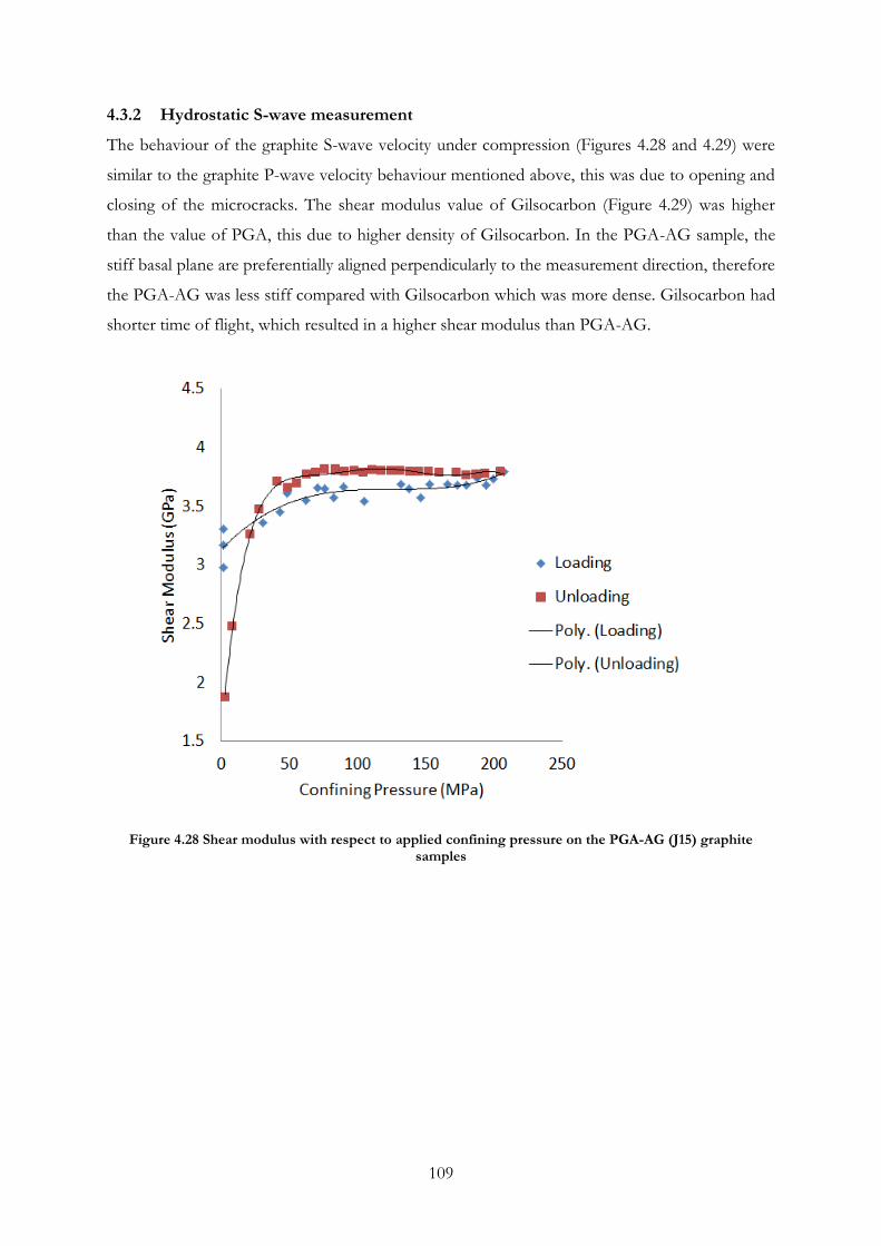
109
4.3.2 Hydrostatic S-wave measurement
The behaviour of the graphite S-wave velocity under compression (Figures 4.28 and 4.29) were
similar to the graphite P-wave velocity behaviour mentioned above, this was due to opening and
closing of the microcracks. The shear modulus value of Gilsocarbon (Figure 4.29) was higher
than the value of PGA, this due to higher density of Gilsocarbon. In the PGA-AG sample, the
stiff basal plane are preferentially aligned perpendicularly to the measurement direction, therefore
the PGA-AG was less stiff compared with Gilsocarbon which was more dense. Gilsocarbon had
shorter time of flight, which resulted in a higher shear modulus than PGA-AG.
Figure 4.28 Shear modulus with respect to applied confining pressure on the PGA-AG (J15) graphite samples

110
Figure 4.29 Shear modulus against applied confining pressure on the Gilsocarbon graphite sample (I5)
4.3.3 Comparison between static and dynamic modulus of PGA and Gilsocarbon
The magnitude of the strain in variation and dynamic experiment was tiny compared to the strain
variation in a static experiment. Also the wave length of the ultrasonic wave was important as
the wavelength must be much larger than the grain size otherwise if the wavelength was too
small it could pass through the material without interacting with the porosity.
As shown by the hydrostatic loading cycles (Figures 4.15 and 4.16), the static stiffness
corresponding to the slope of the loading line was much lower than the dynamic stiffness in the
Figures 4.23 and 4.25- 4.27 that was determined from the ultrasonic velocity measurements.
Upon loading, there are elastic and inelastic deformation occurring whereas upon unloading, the
initial slope corresponded to mostly elastic deformation. Hence the unloading stiffness (as
illustrated in the Figure 4.15 and 4.16) are quite similar to the dynamically measured stiffness
during loading apart from Gilsocarbon dynamic loading stiffness.
4.3.4 Discussion and conclusion
The static and dynamic elastic moduli of the two grades of graphites (PGA and Gilsocarbon)
have been measured for comparison. It was shown that the anisotropy of the elastic properties
of PGA is due to the crystallographic texture formed during the extrusion process, the pores and

111
microcracks are not totally closed at a pressure of 200 MPa and they greatly influence the exact
values of the bulk elastic moduli of graphite. At low pressure, the increase in modulus was
negligible, due to the fact that there was not enough pressure to cause major grain distortion and
porosity. The modulus of the graphite grades increased rapidly in a non-linear manner below and
above a critical pressure, critical pressure referred to as the crack-closure pressure, as the
pressure increased. During loading, the microcracks are closed at critical pressures of ~50 MPa
and ~100 MPa for PGA and Gilsocarbon respectively. The modulus increased sharply after
these critical pressures. During unloading, closed cracks reopened gradually until the critical
pressure was reached. Below the critical pressure, the graphite almost recovered its original
volume at a faster rate. It can be concluded that there was strong stress dependency in the
hydrostatic confining conditions due to closure and opening of microcracks.
4.4 Post-deformation microstructural characterization and properties
measurement
After deformation, the change in microstructure properties was characterized using the x-ray
tomography technique, the helium pycnometer and the mercury porosimeter mentioned in
Chapter 3.
4.4.1 Tomography scans and mercury pycnometry results
Gilsocarbon graphite sample (I8) was scanned before and after hydrostatic deformation, the total
tomography slices for each sample was 1800 slices. One of the middle slices (slice 957 is shown
in the Figure 4.30) was chosen in order to examine the microstructural change. The scan of the
virgin sample is shown in the Figure 4.30A and the scan of the deformed sample is displayed in
the Figure 4.30B. In the deformed scan, the red circled areas showed some of the regions where
there was porosity closure while the green areas showed some of the areas where crack opening
was noticed. Both porosity opening and closure were noticed though out the whole graphite
microstructure (filler and binder). These microstructural changes were responsible for the
behaviour of graphite under high pressure measurement.

112
Figure 4.30 Tomographic scans of Gilsocarbon (I8); (A) before and (B) after cyclic confining pressure of up to 200 MPa. The red circled areas showed some of the regions where there was porosity closure while
the green areas showed some of the areas where crack opening was noticed after deformation.
In order to investigate the porosity changes before and after deformation, Aviso was used to
estimate the equivalent pore diameter of tomography scans of Gilsocarbon sample (I8) before
and after deformation. The same region of interest was analysed in both scans. A volume of
300X300X300 voxels was analysed. The result is shown in the Figure 4.31. The smallest feature
in the tomography scan was 14.6 /pixel. In the Figure 4.31, the equivalent pore diameter
below 51.1 is reduced after deformation. The results indicate that the amount of macropores
have reduced after deformation. The same trend (closure of macropores from pore radius 10 -
100 ) was noticed in the mercury pycnometry result shown in Figure 4.32. It provided
reasonable evidence that confirmed the pore closure seen in the two dimensional image (Figure
4.30). The only limitation to with this approach is that porosity micropores below 14.6
cannot be seen in the scans.

113
Figure 4.31 Frequency of the equivalent pore diameter of Gilsocarbon sample I8 tomography scans before and after deformation
The change in porosity throughout the whole scanned micrograph was investigated further by
using mercury porosimetry to analyse the porosity distribution before and after deformation.
These results are shown in Figures 4.32 and 4.33

114
Figure 4.32 Pore size distribution of virgin and deformed Gilsocarbon graphites (I1 – hydrostatically loaded up to 200 MPa, I3 – hydrostatically loaded up to 200 MPa and differential stressed up to 36 kN, and
I7- hydrostatically loaded up to 80 MPa)
In the Figure 4.32, the broken lines represent the deformed Gilsocarbon while the solid lines
represent the virgin Gilsocarbon. There seems to be a general decrease in the porosity volume of
pores radius 1 – 100 m while increase in the volume of open pore radius <1 m. The sample
I3 was hydrostatically loaded up to 200 MPa and differential stressed up to 36 kN while sample
I7 was loaded up to 80 MPa, the sample I3’s volume of open pore entrance radius 1 - 100 m
seemed to be smaller than the sample I7’s volume of open pore entrance radius 1-100 m. In
both cases, more open pore entrance radius <1 m are produced compared with the virgin
sample. Hydrostatic load up to 200 MPa seemed to have a microcrack formation effect on

115
Gilsocarbon microstructure compared with other loading mode i.e. axial deformation, which
seemed to have closed more microcracks formed by the hydrostatic stress. This behaviour is
strange because axial deformation rather than hydrostatic compaction was expected to induce a
greater microcrack formation effect on the Gilsocarbon microstructure. It is suggested that in
closing the large pores during hydrostatic loading, induced strain heterogeneity caused sites of
high internal stress that opened up pores when the pressure was released. The axial deformation
might have “healed” these sites of high internal stress causing them not to open as micropores
when the stress was released.
4.4.2 Gilsocarbon dynamic Young’s modulus and helium pycnometer results
It can be concluded that the higher the hydrostatic stress (200 MPa), the more microcracks that
formed between the grains and the more closure of macropores resulted in decrease in DYM, by
up to 11 %. In axial deformation, pore size ≥ 1 closed, therefore reduced the DYM by 11.5
%. These results are illustrated in the Table 4.3.
Table 4.3 Change in Gilsocarbon elastic properties at different loading mode (i.e hydrostatic loading, differential stress and dynamic loading)
Elastic properties
Virgin Gilso (GPa)
Low CP up to 80MPa
High CP up to
200MPa
CP of 200MPa
and Axial deformation
E 12.4 -6 % -11 % -11.5 %
G 5.1 -2 % -2 % -6 %
Axial deformation created more shear effect in the Gilsocarbon microstructure due to sliding of
the bassal planes on top of each other in the process of moving the crystal into the neighbour
accomodative void. It is suggested that the bonds between the planes become weaker as the
frictional forces increase resulting in lowering of the shear modulus.
The DYM and the shear modulus of Gilsocarbon (before and after deformation) for all different
loading modes are shown in the Figure 4.33.The DYM value for the deformed samples seemed
to be more reduced than the shear modulus as expected. The Gilsocarbon behaviour seemed to
be independent of porosity compared with PGA (Figures 4.36 and 4.37), this shows that PGA
microstructure is more heterogeneous.

116
Figure 4.33 DYM and shear modulus of Gilsocarbon against the Open Pore Volume (OPV) before and after deformation at different loading modes (i.e. hydrostatic loading, differential stress and dynamic
loading)
In the Figures 4.34 and 4.35, both Virgin and deformed PGA show porosity distribution range
from macropores region to the micropores and mesopores regions. The microstructure of both
deformed samples shows overall reduction in the volume of open pore radius 0.003 – 12 m
compared with the virgin sample. Unlike the Gilsocarbon, there was general reduction PGA-WG
and PGA-AG macropores size < 10 m. This might be due to higher total porosity in PGA than
Gilsocarbon. There seems to be more deformation or collapse in the PGA graphite structure due
to more accommodative void in the PGA microstructure compared with Gilsocarbon which is
denser.
PGA-WG (J22) pore sizes generally decreased more than PGA-AG (J9) under the same loading
condition (confining pressure up to 200 MPa), which suggested that more pores closed in the
PGA-WG sample than PGA-AG. This explained the reason why PGA-AG (F5) sample
appeared to be stiffer than PGA-WG (F1) sample in the Figure 4.14.

117
Figure 4.34 Pore size distribution of virgin and deformed PGA-WG graphites (J2 - hydrostatically loaded up to 200 MPa and differential stressed up to 57 MPa, J22 - hydrostatically loaded up to 200 MPa)

118
Figure 4.35 Pore size distribution of virgin and deformed PGA graphites (J8 - PGA-WG sample hydrostatically loaded up to 200 MPa and differential stressed up to 74 MPa, J9 - PGA-WG sample
hydrostatically loaded up to 200 MPa)
4.4.3 PGA dynamic Young’s modulus and helium pycnometer results
In Table 4.4, E and G represent the DYM and shear moduli parallel to the extrusion direction
(PGA-WG) respectively while E* and G* represent the DYM and shear moduli perpendicular to
the extrusion direction (PGA-AG) respectively. Both DYM and shear modulus of deformed
PGA were ~ 4 times and ~27 times more reduced than the DYM and shear modulus of
Gilsocarbon. This can be associated with the lower porosity in Gilsocarbon than PGA.

119
Table 4.4 Change in PGA elastic properties at different loading mode
Elastic properties
Virgin PGA (GPa)
High CP up to
200MPa
CP of 200MPa
and Axial deformation
E 11.1 -43.1% -43.2%
G 4.2 -40.5% -40.5%
E* 5.9 -44.1 -54.2%
G* 3.3 -54.5% -54.5%
In the Figures 4.36 and 4.37, the open porosity volume of PGA seemed to decrease after
deformation as expected, likewise the DYM values. There was a vague trend of porosity
decreasing after deformation of Gilsocarbon samples (Figure 4.33) compared with PGA samples
(Figures 4.36 and 4.37). Unlike the Gilsocarbon, PGA showed more DYM reduction after
deformation (as expected).

120
Figure 4.36 DYM and shear modulus of PGA-WG against the Open Pore Volume (OPV) before and after deformation at different loading mode
Figure 4.37 DYM and shear modulus of PGA-AG against the Open Pore Volume (OPV) before and after
deformation at different loading mode
4.4.4 Pole figures for PGA
The contoured pole figure plot of virgin PGA was compared with the contoured plot of
deformed sample. The plot is shown in Figure 4.38, only the 0001 plane was considered because

121
it was the only crystallographic plane that shows a strong preferred orientation. It was noted that
a girdle formed across the pole figures in a virgin sample is distorted after hydrostatic loading up
to 200 MPa. The initial strong orientation in the girdle becomes scattered and wider. It is
suggested that the grains oriented parallel to the basal plane are distorted during loading due to
basal sliding with the aid of surrounding spectrum of pores.
Figure 4.38 Pole to basal planes derived from the ODF calculated from the PGA experimental pole figures before and after deformation. Colour scale is in multiples of uniform distribution.
4.4.5 Discussion
There was a general decrease in both DYM and shear modulus of deformed samples by applying
increasing hydrostatic stress. This behaviour was more pronounced in PGA than Gilsocarbon.
The modulus value of PGA decreased by ~ 50 % regardless of being subjected to different
loading mode (i.e. hydrostatic loading, differential stress and dynamic loading) unlike
Gilsocarbon sample which a shows slight decrease by 8 – 10 % for the same modulus. It can be
concluded that the decrease in the modulus of graphite by applying hydrostatic stress is mainly

122
due to crystalline re-orientation and microcrack formation occurring with an increase in stress.
However the contribution of an increase in dislocation density as the stress increases cannot be
ignored. The main mechanism of decrease in DYM by applying hydrostatic stress can be
considered to be dependent on the orientation of the crystallites and of pores in the graphite
relative to the direction of applied stress and the level of applied stress.
4.5 Conclusion
Studying the cause and nature of the changes to the porosity may help to provide a mechanistic
understanding of corresponding changes in graphite’s physical and mechanical properties. This is
essential to assess the structural integrity of graphite components. In this work, hydrostatic
deformation of unirradiated graphite under high pressure was analysed to understand the effect
of porosity on both dynamic and static elasticity. The effect of these porosity changes on
graphite bulk properties has been investigated using the helium and mercury porosimetery
approach, and effective medium models.
The stress- strain relationship of polycrystalline graphite is known for its non-linearity and
hysteresis loops during cyclic loading stressing. During axial loading, within the individual
crystallites, the external stress can lead to a combination of (a) elastic deformation, (b)
irreversible shear (or plastic) deformation, (c) relief of internal stresses, and (d) local stresses
greater than the breaking strength which can cause microcracks. The first two processes cited
above have been used to account for the general shape of the axial stress-strain curves.
In most of the experiments in this work, the deformation was closing porosity despite new
porosity being generated during unloading. The axial stress-strain curve initially is linear with an
elastic behaviour, the pre existing microcracks close during the initial loading of the sample, at
this stage there is no circumferential strain within the sample. During unloading, a large
hysteresis was formed. The stressed grains are relieved; the initially closed pores began to reopen.
It is suggested that during this stage, the volume of pore re-opening superseded the volume of
pores closing, the graphite sample volume almost fully recovered.
In axial compression tests, PGA-AG samples was less stiff than PGA-WG samples. In
hydrostatic compaction tests, the PGA-WG sample deformed more because it has to undergo a
less complicated shape change. This was because the symmetry of their anisotropy is parallel to
the symmetry of its sample
For porous material (graphite samples), measurements have shown that it was possible to
measure Young’s modulus using longitudinal and shear velocities. The estimated values for

123
Young’s modulus agree with the values estimated in previous work [115, 116]. Considering a
density value of 1.765 g/cm3, Young’s modulus of virgin graphite in different directions in
graphite samples varies from 5 to 12 GPa. At higher pressure, the densities of graphite samples
were higher than 1.765 g/cm3 (2.1 g/cm3).
The average Young’s modulus of virgin PGA-AG, PGA-WG, and Gilsocarbon were 5.9 GPa,
11.1 GPa and 12.4 GPa respectively, while previous work has reported Young moduli for PGA
PGA-AG, PGA-WG and Gilsocarbon to be 5.4 GPa, 11.7 GPa and 10.85 GPa respectively
without uncertainty estimates[18]. The modulus parallel to the extrusion direction was greater
than perpendicular to the extrusion direction as shown in the Figure 4.3D. Preferential
orientation of the porosity also contributes to the increase in modulus.
The increase in DYM of the samples with increasing pressure demonstrates the significant
contribution of the internal pores and microcracks to the bulk elastic properties of the graphite
and their anisotropy. The value of the shear modulus is less than the value of the dynamic
Young’s modulus for all materials as expected.
The mercury porosimetry results revealed that plastic deformability of the graphites by
hydrostatic loading can be identified with changes in the pore size resulting from the closing and
shrinking of the pores. It shows that there was more porosity closure in deformed PGA than
deformed Gilsocarbon under the same loading mode, the volume of Gilsocarbon seems to
increase or remain the same due to similar volume of microcracks closing and opening during
deformation. There is a general porosity reduction in deformed PGA. It was quite a difficult task
to study the changes in cracks less than 1 before and after deformation due to structural
damage to the graphite after critical pressure exerted by mercury.
The distortion in graphite crystals after loading can be noted in the XRD pole figure contour
plots. Wide range of porosity in the graphite microstructure and crystallograhic preferred
orientation were suggested to be one of the reasons for an easy migration of crystallites during
loading. There was very little permanent strain in Figure 4.38, therefore more significant change
was not expected.

124
CHAPTER 5
5 Micromechanics modelling
Pore spaces are responsible for most of the differences in the mechanical and physical properties
of graphite [5]. Many attempts have been made in the past to explain the elastic behaviour of
porous materials [74, 76, 77, 119]. Since graphite contains a broad distribution of pore sizes
(from sub-micron to few microns) with irregular shapes, it is more challenging to describe the
elastic behaviour of its complex microstructure. However attempts have been made in this thesis
to understand the effect of porosity change (closure and opening) on apparent bulk modulus (the
slope of pressure-volumetric strain curves calculated as shown in chapter 4).
5.1.1 Elastic of Pore-free aggregate
As a starting point of reference, expected average elastic moduli can be calculated according to
various averaging schemes for an isotropically-textured, pore free graphite aggregate. To do this,
the graphite single crystal constants were obtained from Bosak [21], the elastic bulk moduli and
shear moduli [Voigt Reuss Hill (KVRH, and GVRH), Self-Consistent (KSC, and GSC), Hashin
Shtrikman positive and negative bound (KHS+, and GHS+ , KHS- and GHS-)] was calculated using
equations from Berryman [125, 126] as shown in the Table 5.1.
Table 5.1 Estimated elastic stiffness constants for pore-free, isotropically-textured polycrystalline aggregates of the hexagonal crystals of Graphites A, B [125] and Graphite C (Single crystal constants used in calculations are found in Bosak [21], estimated using equations from Toonder et al. [126] and Berryman
[125]). All units are GPa
Moduli Graphite A Graphite B Graphite C
KR 35.8 35.8 36
KV 286.3 286.3 281
KVRH 161 161 150
KHS- 36.2 42
KHS+ 204.2 204.2
KSC 77.8 88
GR 0.65 9.2 11
GV 217.9 219.4 240
GVRH 109.3 114.3 118
GHS- 1.21 14.8
GHS+ 146.2 148.9
GSC 38.9 52.6

125
The differences in moduli of Graphite A, B and C shown in Table 5.1 calculated according to a
given averaging scheme are due to the different values of single crystal elastic constants reported.
There is a huge difference between Voigt (286.3 GPa) and Reuss (36 GPa) averages for K,
presumably on account of the anisotropy of the single crystals. The Reuss averages are much,
closer to the experimental values extrapolated to zero porosity. Reuss averaging assumes
constant stress in all grains, i.e. like a stack of plates normal to the applied load, whereas Voigt is
constant strain between grains. Reuss averages exactly describes the effective moduli of a
suspension of solid grains in a fluid, and also describes the moduli of shattered materials in
which solid fragments are completely surrounded by the pore fluid [74]. It may be suggested that
the freedoms given by the presence of porosity might make it easier for strain mismatches
between grains to be accommodated. Therefore it may be suggested that the microstructure
better supports a Reuss averaging scheme.
5.1.2 Modelling the influence of porosity
The effect of porosity on bulk modulus was considered by using models such as Voigt Reuss
Hill (VRH), Hashin Shtrikman positive and negative bound (HS+ and HS-) and Koster and
Toksoz (KT) for 2-phase aggregates, considering porosity as the second phase. The Reuss
effective bulk modulus (36 GPa) was used as an effective modulus of graphite at zero porosity.
Pores are then added to the models and the value of effective bulk moduli was extrapolated to
zero porosity. The effect of porosity shapes i.e. needle, sphere, penny and disk shapes were also
analysed. It is worth mentioning again that all these models considered assumed that the solid to
be isotropic and linearly-elastic. Gilsocarbon experimental data was used to compare the
effective medium models because graphite in it is near isotropic. PGA graphite was likewise
compared with KT model (even thou PGA is more anisotropic).
5.1.3 Voigt Reuss Hill (VRH) and Hashin-Shtrikman (HS) bounds
In VRH and HS, the bulk modulus of pore-free material (graphite) was taken to be 36 GPa and
the bulk modulus of void (air) to be 1.01 105 Pa. These were used to calculate the properties of
the porous material over a range of porosities from 0 to 25 %. The results were compared with
the Gilsocarbon experimental data (I3) where the porosity was closed by increasing the confining
pressure. It can be seen in Figure 5.1 that experimentally-observed graphite behaviour
corresponds well with the Reuss and HS- bounds. Although Gilsocarbon sample (I3) was
hydrostatically loaded up to 200 MPa and then differential stressed up to 36 kN, only the data
obtained from the hydrostatic compression up to 202 MPa (loading data without unloading) was

126
used in Figure 5.1. These models confirmed that the bulk modulus increased as the porosity
decreased, as expected for porous materials. However this was not entirely true in the case of
graphite, it has also been reported earlier in this work that during loading, microcracks also
formed between the grains (i.e. in the Figure 4.26 in the result chapter)
Figure 5.1 Bulk modulus against porosity for the Voigt, Reuss, HS- and HS+ averaging schemes compared with the experimental data for the Gilsocarbon sample (I3)–hydrostatically loaded up to 202 MPa (loading
data only). The I3 experimental data conform closely to the predictions of Reuss and HS- averaging scheme.
5.2 Kuster and Toksoz model
The Kuster and Toksoz (K-T) formulation for effective moduli was used to calculate the effect
of porosity on effective bulk modulus as shown in the Figures 5.2 and 5.3. The bulk modulus
curve increases rapidly below 14 % and 25 % porosity closure in Figures 5.2 and 5.3 respectively.
There was not enough pressure to close all the pores in the graphite sample, but it shows
continuous increase in bulk modulus at lower porosity. Bulk modulus of non-porous
Gilsocarbon can be calculated from the work of Berre [14, 120] to be 8.3 GPa, and this has
It was found that porosity in the form of penny-shaped cracks of aspect ratio 0.003, coupled
with a zero-porosity bulk modulus of 8.3 GPa gave the best fit with the experimental data for

127
Gilsocarbon sample I3 for the porosity range 15 – 8 % (Figure 5.2). The value for zero porosity
bulk modulus that has to be assumed is lower than any predicted from single-crystal elastic
averaging schemes (Table 5.1), and this is a weakness of this approach.
Figure 5.2 Bulk modulus against porosity of the KT model for the crack aspect ratio shown and a zero-porosity modulus of 8.3 GPa, compared with the experimental data for the Gilsocarbon sample (I3)–
hydrostatically loaded up to 202 MPa (loading data only)
In Figure 5.3, the KT model slope of 50 % of penny cracks with aspect ratio 0.01 and 50 %
sphere porosity was used to fit the PGA sample (J9) experiment data (seismic loading up to 207
MPa). The KT model slope is less steeper than the PGA data. The difference between the model
and PGA sample (J9) can also be associated with the porosity interaction in the graphite. Based
on the KT model shown in Figures 5.2 and 5.3, it may be suggested that there are more penny
cracks with lower aspect ratio (0.003) in Gilsocarbon than PGA sample. The 50 % spherical
porosity in Figure 5.3 suggested the presence of large pore size in PGA than Gilsocarbon.

128
Figure 5.3 DYM against porosity of the KT model for the crack aspect ratio shown and sphere porosity compared with the experimental data for the DYM of PGA sample (J9) – seismic loaded up to 202 MPa
(loading data only)
5.3 Conclusion
Models to estimate the mechanical properties of graphites over a wider range of porosity than
was accessible from the experimental studies were attempted using effective medium (EM)
models. Voigt, Reuss, Hill, Hashin-Shtrikman bounds and Kuster and Toksoz models have been
used. None of the models can completely describe all the characteristics of the experimental
data; this might be due to porosity interaction in the graphite during deformation. Since the
model theories did not explicitly consider the interaction of pores within their medium, they are
not completely reliable representatives of the complex change in graphite macrostructure.
However, the Reuss averaging scheme for porous graphite, using a Reuss average bulk modulus
from single crystal elastic moduli determinations, or the KT scheme for an assumed value of
zero-porosity bulk modulus and an assumed crack porosity aspect ratio, provide good fits to the
experimental data for Gilsocarbon, and therefore can be used as a satisfactory semi-empirical

129
basis for calculating effective moduli for porosities outside the experimental range of 8 to 15%
porosity.

130
CHAPTER 6
6 Summary, conclusions and further work
The aim of this work was to use hydrostatic pressure to study possible synergies with the elastic
behaviour of irradiated graphite Although the nuclear reactor environmental condition is harsh
(e.g. high temperature), the effect of temperature on graphite was not investigated in this work.
Thus the investigation of possible time-dependent behaviour which might rise as a result of
thermally activated deformation processes could not be investigated. Time dependent behaviour
could not be seen at room temperature. Hence this is a key area for future research.
Despite carrying out this study only at room temperature, we can recognize that since irradiation
changes are primarily related to crystallite reorientation and opening and closure of porosity,
these changes can be successfully simulated by hydrostatic compaction of graphite. In this study,
modulus increases due to application of pressure have been shown to be related to measured
microstructural changes. In the same way, modulus changes induced in graphite through
irradiation can be linked to microstructural changes. We can therefore postulate that whether
given microstructural changes are induced either by hydrostatic pressure or by irradiation, similar
elastic property changes can be expected..
The elastic properties of graphite can change in a nuclear reactor because cumulative damage can
lead to graphite shrinkage, potentially resulting in disengagement of individual components and
loss of core geometry. Differential shrinkage in the graphite component can lead to the
generation of internal stresses and component failure by cracking.
In the course of this study a range of experimental measurements of the effects of hydrostatic
and non-hydrostatic loading on isotropic and anisotropic graphites was brought to bear, in order
to link the effects to microstructural changes, and this represents the principal scientific
contribution of the present research. These studies were:
The porosity and pore-size distributions and the crystallite orientation in the graphite
microstructure were characterized before and after deformation. It was confirmed that
Gilsocarbon is near isotropic, as shown by the pole figure uniform intensity. The PGA
pole figure showed a strong girdle of poles to basal planes, which confirmed its
anisotropic nature. Deformed graphite showed increased scatter of orientations but the
initial girdle texture remained.

131
Through carrying out hydrostatic compaction experiments coupled with dynamic
modulus measurement on nuclear graphite samples. The author was able to demonstrate
quantitatively that the increase in Young’s modulus is due to porosity closure.
Application of effective medium models showed the importance of porosity evolution in
the graphite during deformation. Graphite is extremely anisotropic, to the extent that the
Voigt (isostress) and Reuss (isostrain) averages are so different that they are likely not to
be meaningful in an anisotropic material. The question therefore arises “what kind of
averaging scheme can be usefully applied?” so that elastic property changes can be linked
to microstructural changes extrapolated outside the range of experimental measurements.
A range of elastic property averaging schemes was applied. The heart of this is zero porosity
elastic behaviour, because that pins the curves shown in Figures 5.1 and 5.2. The Reuss averages
(e.g. 36 GPa for the bulk modulus) were found to be much closer to the experimental values
extrapolated qualitatively to zero porosity. Incorporating the effects of porosity using either the
Reuss or Kuster/Toksoz averging schemes was shown to provide a useful semi-empirical basis
for extrapolating the effects of porosity outside the range of experimental data.
Studying the cause and nature of the changes to the porosity has helped to provide a mechanistic
understanding of corresponding changes in physical and mechanical properties of graphite. Thus
observations of the microstructural changes caused to irradiated graphite components can be
translated into corresponding effects on elastic properties using the approach developed in this
thesis.
6.1 Potential future research directions are outlined below
When graphite is irradiated, its Young’s modulus first rises rapidly, then increases more
slowly before falling off towards zero with increasing fast neutron fluence (time
irradiated). This behaviour is thought to be associated with dislocation pinning, crack
closure and finally grain boundary cracking, but no real evidence of this behaviour
presently exists is in the literature. The author recommends that future work should
involve the investigation of the change in porosity, in graphite irradiated to various levels
of irradiation dose, by measuring pore volume change as a function of confining pressure
between room temperature to 700°C, in order to study more directly the effects of
irradiation and temperature on porosity change. This could be coupled with dynamic
modulus measurement.

132
In carrying out the mercury porosimeter measurements, it proved difficult to study the
closure of cracks less than 1 before and after deformation due to the graphite
structural damage after critical pressure is reached during mercury porosimetry.
Furthermore the use of the helium porosimeter in this work could only measure the total
accessible pore volume. The pore size distribution could not be measured. It would be
better to characterise the pore distribution using a Quantachrome gas porosimeter which
is capable of measuring pore distribution in pores less than 1 using a gas medium.
XRD has low penetration power and small beam size compared with neutron diffraction
techniques, and pore statistics can be achieved in coarse-grain materials. A complete pole
figure cannot be measured by laboratory X-ray diffraction due to the strong defocusing
effect and diffraction geometry as mentioned earlier in Chapter 3. Electron diffraction
maybe a better candidate method; [ but you can only do this in very thin specimens, do
you really want to suggest this, except only for EBSD texture measurements?] the result
from electron diffraction can be presented directly in orientation space without the
additional mathematical calculations which are necessary in X-ray and neutron
measurements. Possible errors occurring during mathematical treatments can be avoided
using electron diffraction. However the author did not use a Scanning Electron
Microscope (SEM) equipped with an Electron Backscatter Diffraction (EBSD) detector,
because it was very difficult to polish the samples. Ion beam milling might be an option
to polish the surface, although it takes a long time to do so given the area that would be
required to include enough grains. Another option is chemical polishing but graphite is
so unreactive it might be difficult to form a good polished surface.
In-situ measurements (e.g. using high-energy synchrotron radiation) are capable of
revealing microstructure and texture evolution in the sample being tested. This would
avoid the uncertainty originating from the usage of many different samples. The
mechanical properties and texture evolution are strongly dependent on the initial texture
and microstructure. By interpreting the measured texture results together with the results
of a numerical simulation of texture development, the anisotropic behaviour and the
activity of the potential deformation modes in a graphite microstructure could be
analysed as a function of initial texture and degree of deformation.
Multi-scale modelling using finite element analysis would also be attempted. This might
be used to model more directly the mechanistic behaviour of graphite non-linearity, by
using tomography scans to create a realistic finite element model and using Simpleware

133
CAD software. It should be aimed to create models with realistic, but simplified, ideal
pores which may interact. The apparent bulk modulus calculated in such away can be
compared with experimental results.
Studies of evolution of mechanical properties should be carried out at high temperatures,
more closely to simulate the in-reactor condition, due to investigate thermally-activated
deformation processes.

134
7 Appendix
Table 7.1 Summary of data reported in the text for Gilsocarbon graphites ( K is the bulk modulus, whilst K after is the bulk moduli after deformation E is the dynamic moduli, whilst E after is the dynamic moduli after deformation, G is the shear moduli whilst G after is the shear moduli after deformation).
ID Porosity CPV OPV OPV after porosity
after E
(GPa) G
(Gpa) E after (GPa)
G after (GPa) V1 V2 K= E/3(1-2V)
K after (GPa)
I7 16.8 7.1 9.7 9.3 16.4 12.3 5 11.6 4.9 0.23 0.18 7.59 6.11
E1 19.6 9.1 10.5 10.3 19.4 12.5 5.1 11.21 5.18 0.23 0.08 7.59 4.47
E2 19.6 9.5 10.1
9.5 12.3 5
0.23
7.59 I1 20.7 8.5 12.2 11.9 20.4 12 5 11.1 4.9 0.20 0.13 6.67 5.04
I4
9.7
12.4 5 11.2 4.6 0.24 0.22 7.95 6.61
I5
7
12.3 5 11.1 4.6 0.23 0.21 7.59 6.30
I6 16.9 7.3 9.6 9.3 16.6 12.5 5 12 5.3 0.25 0.13 8.33 5.44
I8 17.6 7.6 10 10 17.6 12.2 5 10.4 4.4 0.22 0.18 7.26 5.45
I10 19.1 7.1 12 9.7 16.8 12.3 5.1
0.21
6.97 I2 19.6 8.6 11 10.9 19.5 12.3 5 11.2 5 0.23 0.12 7.59 4.91
I3 19.2 8.7 10.5 10.3 19 12.2 5 10.8 4.7 0.22 0.15 7.26 5.13

135
8 References
1. Greenstreet, W.L., et al., The mechanical behavior of artificial graphites as portrayed by uniaxial tests. Carbon, 1970. 8(5): p. 649-663.
2. Jones A N, M.B.J., Marrow T J, Microstructural Characterisation of Nuclear Grade Graphite using High Resolution Techniques, in 7th International Nuclear Graphite Specialists Meeting (INGSM-8). 2007, Materials Performance Centre: Bakubung, South Africa.
3. Teresa Telesco, K.B., Critical Technology Assessment: fine grain, high density graphite, U.S.D.o. Commerce, Editor. 2010: Washington D.C.
4. Fazluddin, S., Crack growth resistance in nuclear graphite, in Department of Materials. 2002, University of Leeds: Leeds.
5. Kelly, B.T., Physics of graphite 1981, London: Applied Science Publishers. 6. Kelly, B.T., D. Jones, and A. James, Irradiation damage to pile grade graphite at 450° C.
Journal of Nuclear Materials, 1962. 7(3): p. 279-291. 7. Oku, T. and M. Eto, Relation between static and dynamic Young's modulus of nuclear graphites and
carbon. Nuclear Engineering and Design, 1993. 143(2–3): p. 239-243. 8. B. T. Kelly, W.H.M., A. M. Price, J. T. Bland The mechanism of dimensional changes in the
crystals of graphites and carbons under fast neutron irradiation in Philosophical Magazine. 1966. p. 343- 356.
9. Price, R.J., Strength of Irradiated graphite, in General atomic project 6400, G.a. company, Editor. 1979, U.S department of energy: United State.
10. Kelly, B.T., The structure and manufacture of nuclear grade graphite, Irradiation damege in graphite due to fast neutrons in fission and fussion systems, IAEA, Editor. 2000: Austria.
11. Hall, G., et al. Possibility for the microstructural modelling of the irradiation properties of graphites for future high temperature reactors. in 3rd International Topical Meeting on High Temperature Reactor Technology. 2006. Johannesburg, South Africa: Proceedings HTR2006.
12. Brocklehurst, J.E., Adam, R.W. , Mechanical tests on graphite with simulated radiolytic oxidation gradients, UKAEA, Editor. 1983: Warrington. p. 1-38.
13. Brocklehurst, J.E., A method of simulating graphite property changes caused by radiolytic oxidation (for application to realistic tests on moderator bricks), UKAEA, Editor. 1980, Springfields Nuclear Power Development Laboratories: Preston. p. 1-21.
14. Berre, C., et al., Numerical modelling of the effects of porosity changes on the mechanical properties of nuclear graphite. Journal of Nuclear Materials, 2006. 352(1-3): p. 1-5.
15. D.Buckthorpe, R.C., B. Van der Schaaf, B. Riou, H. Rantala, R. Moormann, F. Alonso, B-C. Friedrich, Materials for High Temperature Reactor (HTR), in 16th Structural Mechanics in Reactor Technology (SMiRT 16). 2001, International & American Associations for Structural Mechanics in Reactor Technology Washington DC.
16. Pierson, H.O., Handbook of Carbon, Graphite, Diamond and Fullerenes - Properties, Processing and Applications. 1993: William Andrew Publishing/Noyes.
17. Francis, I.T., K.R. A Thoms, and A.F. A Rowcliffe, Neutron irradiation experiments for fission and fusion reactor materials studies. Journal of Neutron Research, 1994. 2(2): p. 71- 83.
18. Marsden, B.J. Graphite Technology Course. 2002; Available from: http://pbadupws.nrc.gov/docs/ML0120/ML012080125.pdf.
19. Bernal, J.D., The Structure of Graphite. Proceedings of the Royal Society of London. Series A, Containing Papers of a Mathematical and Physical Character, 1924. 106(740): p. 749-773.
20. Hall, G.N., Microstructure modelling of Nuclear grade graphite, in MACE. 2004, University of Manchester: Manchester. p. 352.

136
21. Bosak, A., et al., Elasticity of single-crystalline graphite: Inelastic x-ray scattering study. Physical Review B, 2007. 75(15): p. 153408.
22. Kwiecinska, B. and H.I. Petersen, Graphite, semi-graphite, natural coke, and natural char classification--ICCP system. International Journal of Coal Geology, 2004. 57(2): p. 99-116.
23. Reynolds, W.N., Physical properties of graphite. 1968, Amsterdam, New York Elsevier Pub. Co. .
24. Ebert, L.B., Intercalation Compounds of Graphite. Annual Review of Materials Science, 1976. 6: p. 181-211.
25. Nightingale, R.E., Nuclear graphite. 1962, New York: Academic press. 26. Rand, S.J., Significance of Tests for Petroleum Products (7th Edition): (MNL 1). 2003: ASTM
International. 27. Robert, B., NGNP Graphite Testing and Qualification Specimen Selection Strategy. 2005. p.
Medium: ED. 28. Ragan, S. and H. Marsh, Review Science and technology of graphite manufacture. J. Mat. Sc.,
(1983). 18( ): p. 3161—3176. 29. Vreeling, J.A., O. Wouters, and J.G.v.d. Laan, Graphite irradiation testing for HTR technology
at the High Flux Reactor in Petten. Journal of Nuclear Materials, 2008. 381(1-2): p. 68-75. 30. Snead, L.L., T.D. Burchell, and Y. Katoh, Swelling of nuclear graphite and high quality carbon
fiber composite under very high irradiation temperature. Journal of Nuclear Materials, 2008. 381(1-2): p. 55-61.
31. Fazluddin, S., Crack growth resistance in nuclear graphite, in School of Process, Environmental and Materials Engineering. 2002, The University of Leeds: Leeds. p. 248.
32. Chi, S.-H., Specimen size effects on the compressive strength and Weibull modulus of nuclear graphite of different coke particle size: IG-110 and NBG-18. Journal of Nuclear Materials, (0).
33. Fedorchenko, B., I. I, Nenakhov, A. V, Beloivan, A. F., Mechanical properties of composite materials based on polyfluoroethylene resin. Strength of Materials, 1971. 3(10): p. 1204- 1207.
34. Hall, G., B.J. Marsden, and S.L. Fok, The microstructural modelling of nuclear grade graphite. Journal of Nuclear Materials, 2006. 353(1-2): p. 12-18.
35. Libin Sun, A.H., James Marrow, Alex SL Fok and Barry J Marsden, AN EXPERIMENTAL STUDY ON THE POROSITY NETWORKS IN NUCLEAR GRAPHITE, in 2nd International Topical Meeting on HIGH TEMPERATURE REACTOR TECHNOLOGY. 2004: Beijing, CHINA.
36. Wen, K.Y., T.J. Marrow, and B.J. Marsden, The microstructure of nuclear graphite binders. Carbon, 2008. 46(1): p. 62-71.
37. Zdravkov, B., et al., Pore classification in the characterization of porous materials: A perspective. Central European Journal of Chemistry, 2007. 5(2): p. 385- 395.
38. J.F. Byrne, H.M., ed. Porosity in Carbons. first ed. Characterization and Applications, ed. W. Patrick. 1995, Halsted Press: London.
39. Neighbour, G.B., ed. Management of ageing processes in graphite reactor cores. 2007, The Royal Society of Chemistry: UK.
40. Tsang, D.K.L. and B.J. Marsden, The development of a stress analysis code for nuclear graphite components in gas-cooled reactors. Journal of Nuclear Materials, 2006. 350(3): p. 208-220.
41. Sutton, A.L. and V.C. Howard, The role of porosity in the accommodation of thermal expansion in graphite. Journal of Nuclear Materials. 7(1): p. 58-71.
42. Seldin, E.J., Stress-strain properties of polycrystalline graphites in tension and compression at room temperature. Carbon, 1966. 4(2): p. 177-191.
43. Jenkins, G.M., The stress-strain relationships of polycrystalline graphite under compression up to fracture. Carbon, 1965. 3(1): p. 93-94.
44. Jenkins, G.M., Analysis of the stress-strain relationships in reactor grade graphite. Br. J. Appl. Phys. 13 30.

137
45. Jenkins, G.M., The effect of microporosity on the elastic modulus and yield curve of polycrystalline graphite. Journal of Nuclear Materials, 1969. 29(3): p. 322-328.
46. Spriggs, R.M., Expression for Effect of Porosity on Elastic Modulus of Polycrystalline Refractory Materials, Particularly Aluminum Oxide. Journal of the American Ceramic Society, 1961. 44(12): p. 628-629.
47. Hasselman, D.P.H., On the Porosity Dependence of the Elastic Moduli of Polycrystalline Refractory Materials. Journal of the American Ceramic Society, 1962. 45(9): p. 452-453.
48. Hashin, Z., The Elastic Moduli of Heterogeneous Materials. Journal of Applied Mechanics, 1962. 29(1): p. 143-150.
49. Boey, S.Y. and D.J. Bacon, Deformation of polycrystalline graphite under pressure. Carbon, 1986. 24(5): p. 557-564.
50. Brocklehurst, J.E., et al., The effect of radiolytic oxidation on the physical properties of graphite. J. Nucl. Mat., (1970). 35 p. 183—194.
51. Jenkins, G.M., Fracture in reactor graphite. Journal of Nuclear Materials, 1962. 5(3): p. 280-286.
52. O. D, S., Deformation Mechanisms in Polycrystalline Graphite. Journal of the American Ceramic Society, 1967. 50(10): p. 495.
53. Oku, T. and M. Eto, The effect of compressive prestressing on the mechanical properties of some nuclear graphites. Carbon, 1973. 11(6): p. 639-647.
54. Paterson, M.S. and J.M. Edmond, Deformation of graphite at high pressures. Carbon, 1972. 10(1): p. 29-34.
55. Kmetko, E.A., J.R. Morgan, and J.F. Andrew, The compressibility of synthetic polycrystalline graphite and the effect of pore Structure accessibility. Carbon, 1968. 6(4): p. 571-572.
56. Yoda, S., I. Ioka, and M. Eto, Deformation of graphites under hydrostatic states. Journal of Nuclear Materials, 1984. 125(1): p. 113-116.
57. Union Carbide, C., The industrial graphite engineering handbook. 1959, New York: Union Carbide.
58. Kelly, B.T., Graphite--the most fascinating nuclear material. Carbon, 1982. 20(1): p. 3-11. 59. Narisawa, M., M. Adachi, and I. Souma, High-temperature creep and resultant anisotropy in
ultrasonic velocity in isotropic graphite. Journal of Materials Science, 1994. 29(3): p. 708-713. 60. Kelly, B.T., W.H. Martin, and P.T. Nettley, Dimensional Changes in Polycrystalline Graphites
under Fast-Neutron Irradiation. Philosophical Transactions of the Royal Society of London. Series A, Mathematical and Physical Sciences, 1966. 260(1109): p. 51-71.
61. Burchell, T.D. and L.L. Snead, The effect of neutron irradiation damage on the properties of grade NBG-10 graphite. Journal of Nuclear Materials, 2007. 371(1-3): p. 18-27.
62. Marsden, B.J., S.-L. Fok, and H. Li, Irradiation behaviour and structural analysis of HTR/VHTR graphite core component, in 18th Internation Conference on Structural Mechanics in Reactor Technology (SMiRT 18). 2005, SMiRT: Beijing, China.
63. Gateau, Measurement of the physical and mechanical properties of pressed Gilsocarbon graphite, in O.E.C.D. High temperature reactor project, D.p. report, Editor. 1989: Paris.
64. Mason, I.B. and R.H. Knibbs, The Young's modulus of carbon and graphite artefacts. Carbon, 1967. 5(5): p. 493-506.
65. Pickup, I.M., B. McEnaney, and R.G. Cooke, Fracture processes in graphite and the effects of oxidation. Carbon, 1986. 24(5): p. 535-543.
66. Standring, J. and B.W. Ashton, The effect of radiolytic oxidation by carbon dioxide on the porosity of graphite. Carbon, 1965. 3(2): p. 157-165.
67. Best, J.V., W.J. Stephen, and A.J. Wickham, Radiolytic graphite oxidation. Progress in Nuclear Energy, 1985. 16(2): p. 127-178.
68. Kelly, B.T., et al., The annealing of irradiation damage in graphite. Journal of Nuclear Materials, 1966. 20(2): p. 195-209.

138
69. Kelly, B.T., et al., U.K.A.E.A. northern division studies of the radiolytic oxidation of graphite in carbon dioxide. Carbon, 1983. 21(4): p. 441-449.
70. Knudsen, F.P., Dependence of Mechanical Strength of Brittle Polycrystalline Specimens on Porosity and Grain Size. Journal of the American Ceramic Society, 1959. 42(8): p. 376-387.
71. Engle, G.B., Density and structural distributions in artificial graphites. Carbon, 1970. 8(4): p. 485-495.
72. Freise, E.J. and A. Kelly, Twinning in Graphite. Proceedings of the Royal Society of London. Series A, Mathematical and Physical Sciences, 1961. 264(1317): p. 269-276.
73. Kuster, G. and M. Toksöz, Velocity and attenuation of seismic waves in two phase media: Part II. Experimental results GEOPHYSICS, 1974. 39(5): p. 607-618.
74. Mavko, G., T. Mukerji, and J. Dvorkin, The rock physics handbook: tools for seismic analysis in porous media. 1998: Cambridge Univ. Press.
75. Hill, R., The elastic behaviour of crystalline aggregate. Proceedings of the Physical Society, 1952. 65: p. 349.
76. Berryman, J.G., Long-wavelength propagation in composite elastic media II. Ellipsoidal inclusions. The Journal of the Acoustical Society of America, 1980a. 68(6): p. 1809-1819.
77. Berryman, J.G., Long-wavelength propagation in composite elastic media II. Ellipsoidal inclusions. The Journal of the Acoustical Society of America, 1980b. 68(6): p. 1820-1831.
78. Mavko, G., Effective medium theories, in Effective medium models, S.r.p. laboratory, Editor. 2009, Stanford university: California. p. 113-163.
79. Eto, M. and T. Oku, Change in electrical resistivity of nuclear graphite during compression tests and a model for its deformation and fracture mechanism. Journal of Nuclear Materials, 1974. 54(2): p. 245-253.
80. Eto, M. and T. Oku, The effect of pre-stressing and annealing on the young's modulus of some nuclear graphites. Journal of Nuclear Materials, 1973. 46(3): p. 315-323.
81. Yoda, S., M. Eto, and I. Ioka, Effects of prehydrostatic loading on mechanical and physical properties of nuclear-grade graphites. Journal of Nuclear Materials, 1984. 125(1): p. 104-110.
82. Brocklehurst, J.E. and B.T. Kelly, Analysis of the dimensional changes and structural changes in polycrystalline graphite under fast neutron irradiation. Carbon, 1993. 31(1): p. 155-178.
83. Pierre Ouagne, G.B.N., Brian McEnaney, Influence of oxidation on toughness parameters for two nuclear grade graphites. Journal of Physics D: Applied Physics, 2005. 38: p. 1259-1264.
84. Fazluddin Shahed (2002) . PhD thesis, Crack growth resistance in nuclear graphite, in Department of Materials. 2002, University of Leeds: Leeds.
85. Svalbonas, V., T.C. Stilwell, and Z. Zudans, Rules for design of nuclear graphite core components — Some considerations and approaches. Nuclear Engineering and Design, 1978. 46(2): p. 313-333.
86. P.Beghein, G.B., F.Hiltmann, M.Melin and B.du Mesnildot. Nuclear Graphite NBG-17 and other solutions for the nuclear industry. in INGSM- 11. 2010. Eastbourne, UK.
87. Cortie, M.B., Calculation of Texture Volume Fractions by Integration and Gaussian Fitting. Textures and Microstructures, 1997. 29(3-4): p. 155-183.
88. L.Sun, et al. An Experimental Study on The Porosity Networks In Nuclear Graphite. in Proceedings of the Conference on High Temperature Reactors. 2004. Beijing, China: International Atomic Energy Agency.
89. Babout, L., et al., The effect of thermal oxidation on polycrystalline graphite studied by X-ray tomography. Carbon, 2005. 43(4): p. 765-774.
90. John, C.R., The Image Processing Handbook, Fifth Edition (Image Processing Handbook). 2006: CRC Press, Inc.
91. Kocks, U.F., C.N. Tomé, and H.R. Wenk, Texture and Anisotropy: Preferred Orientations in Polycrystals and Their Effect on Materials Properties. 2000: Cambridge University Press.
92. Bacon, G.E., A method for determining the degree of orientation of graphite. Journal of Applied Chemistry, 1956. 6(11): p. 477-481.

139
93. Harold P. Klug, L.E.A., X-Ray Diffraction Procedures: For Polycrystalline and Amorphous Materials. 2nd ed. 1974, New York: J. Wiley.
94. Hammond, C., The Basics of Crystallography and Diffraction. 2001: Oxford University Press. 95. Bunge, H.J., Texture analysis in materials science : mathemat. methods. 1982, London u.a.:
Butterworth. 96. Segmuller, A. and J. Angilello, Automatic pole figure evaluation. Journal of Applied
Crystallography, 1969. 2(2): p. 76-80. 97. Hielscher, R. and H. Schaeben, A novel pole figure inversion method: specification of the MTEX
algorithm. Journal of Applied Crystallography, 2008. 41(6): p. 1024-1037. 98. F. Bachmann, R.H., Helmut Schaeben, Texture Analysis with MTEX- Free and open source
software toolbox. Solid state Phenomena, 2010. 160: p. 63-68. 99. Krigbaum, W.R. and A.M.H. Vasek, A Test of the Refinement Procedure for Determining the
Crystallite Orientation Distribution: Polyethylene Terephthalate. Texture, 1972. 1(1): p. 9-16. 100. R.-J. Roe, W.R.K., Description of crystallite orientation in polycrystalline material having fiber texture.
Journal of of Chemical Physics, 1964. 40(9): p. 8. 101. R.-J. Roe, Description of crystallite orientation in polycrystalline materials. III. General solution to pole
figure inversion. Journal of Applied Physics, 1965. 36(6). 102. Matthies, S., G.W. Vinel, and K. Helming, Standard distributions in texture analysis. 1900,
Berlin: Akademie-Verlag. 103. Keng, E.Y.H., Air and Helium Pycnometer. Powder Technology, 1969. 3(3): p. 179-180. 104. Lowell, S., Characterization of Porous Solids and Powders: Surface Area, Pore Size, and Density.
2004: Kluwer Academic Publishers. 105. Ciftcioglu, M., D.M. Smith, and S.B. Ross, Mercury porosimetry of ordered sphere compacts:
Investigation of intrusion and extrusion pore size distributions. Powder Technology, 1988. 55(3): p. 193-205.
106. Dickinson, J.M. and J.W. Shore, Observations concerning the determination of porosities in graphites. Carbon, 1968. 6(6): p. 937-941.
107. http://www.quantachrome.co.uk/en/Automatic_Pore_Size_Analyzers-Poremaster.asp. 108. Goodman, R.E., Introduction to Rock Mechanics (2nd Edition), John Wiley & Sons. 109. Yoda, S., M. Eto, and T. Oku, Change in dynamic young's modulus of nuclear-grade isotropic
graphite during tensile and compressive stressing. Journal of Nuclear Materials, 1983. 119(2-3): p. 278-283.
110. Asmani, M., et al., Influence of porosity on Young's modulus and Poisson's ratio in alumina ceramics. Journal of the European Ceramic Society, 2001. 21(8): p. 1081-1086.
111. Thrower, P.A., The structure of reactor graphites and its relation to high temperature irradiation dimensional stability. Carbon, 1971. 9(3): p. 265-277.
112. Lokajicek, T., et al., The determination of the elastic properties of an anisotropic polycrystalline graphite using neutron diffraction and ultrasonic measurements. Carbon, 2011. 49(4): p. 1374-1384.
113. James G, B., Bounds and self-consistent estimates for elastic constants of random polycrystals with hexagonal, trigonal, and tetragonal symmetries. Journal of the Mechanics and Physics of Solids, 2005. 53(10): p. 2141-2173.
114. Williams, W.J., Mercury porosimetry studies on PGA, AGL-mp and BAEL-GCMB Graphites. 1976, Berkeley Nuclear Laboratories: Berkeley, Gloucestershire.
115. Vidal, J.M., Mays, T.J., Mechanical properties and oxidation of nuclear graphites. 1999, Department of Material Science and Engineering, University of Bath: Bath.
116. IAEA, Characterization, treatment and conditioning of radioactive graphite from decommissioning of nuclear reactors, in Waste technology section. 2006, IAEA: Vienna. p. 1-71.
117. Abrahamson, J., The surface energies of graphite. Carbon, 1973. 11(4): p. 337-362. 118. Eto, M., T. Oku, and T. Konishi, High temperature young's modulus of a fine-grained nuclear
graphite oxidized or prestressed to various levels. Carbon, 1991. 29(1): p. 11-21.

140
119. Barsoum, M.W., et al., Kink bands, nonlinear elasticity and nanoindentations in graphite. Carbon, 2004. 42(8–9): p. 1435-1445.
120. ChristopheBERRE, Microstructural modelling of nuclear graphite using X-ray micro-tomography data, in School of Mechanical, Aerospace and Civil Engineering. 2007, University of Manchester: Manchester. p. 223.
121. Pros, Z., et al., Direct measurement of 3D elastic anisotropy on rocks from the Ivrea zone (Southern Alps, NW Italy). Tectonophysics, 2003. 370(1–4): p. 31-47.
122. Kern, H., et al., The effect of oriented microcracks and crystallographic and shape preferred orientation on bulk elastic anisotropy of a foliated biotite gneiss from Outokumpu. Tectonophysics, 2008. 457(3–4): p. 143-149.
123. Blakslee, O.L., et al., Elastic Constants of Compression‐Annealed Pyrolytic Graphite. Journal of Applied Physics, 1970. 41(8): p. 3373-3382.
124. Faulkner, D.R. and E.H. Rutter, Comparisons of water and argon permeability in natural clay-bearing fault gouge under high pressure at 20°C. Journal of Geophysical Research: Solid Earth, 2000. 105(B7): p. 16415-16426.
125. Berryman, J.G., Bounds and self-consistent estimates for elastic constants of random polycrystals with hexagonal, trigonal, and tetragonal symmetries. Journal of the Mechanics and Physics of Solids, 2005. 53(10): p. 2141-2173.
126. Den Toonder, J.M.J. and Toonder, The relation between single crystal elasticity and the effective elastic behaviour of polycrystalline materials: theory, measurement and computation. Modelling and Simulation in Materials Science and Engineering, 1999. 7(6): p. 909.


![Earthquake-induced deformation analyses of the Upper San ...5] BKP P m = ′ ba m a σ where B is the bulk modulus, Kg is the shear modulus con-stant, n is the shear modulus exponent](https://static.fdocuments.in/doc/165x107/5ecc9e3b3fff8c554e0e2d22/earthquake-induced-deformation-analyses-of-the-upper-san-5-bkp-p-m-a-ba.jpg)