Definition of the Semisubmersible Floating System for ... · Definition of the Semisubmersible...

NREL is a national laboratory of the U.S. Department of Energy Office of Energy Efficiency & Renewable Energy Operated by the Alliance for Sustainable Energy, LLC This report is available at no cost from the National Renewable Energy Laboratory (NREL) at www.nrel.gov/publications.

Contract No. DE-AC36-08GO28308

Definition of the Semisubmersible Floating System for Phase II of OC4 A. Robertson, J. Jonkman, M. Masciola, and H. Song National Renewable Energy Laboratory

A. Goupee and A. Coulling University of Maine

C. Luan Norwegian University of Science

Technical Report NREL/TP-5000-60601 September 2014

NREL is a national laboratory of the U.S. Department of Energy Office of Energy Efficiency & Renewable Energy Operated by the Alliance for Sustainable Energy, LLC This report is available at no cost from the National Renewable Energy Laboratory (NREL) at www.nrel.gov/publications.

Contract No. DE-AC36-08GO28308

National Renewable Energy Laboratory 15013 Denver West Parkway Golden, CO 80401 303-275-3000 • www.nrel.gov

Definition of the Semisubmersible Floating System for Phase II of OC4 A. Robertson, J. Jonkman, M. Masciola, and H. Song National Renewable Energy Laboratory

A. Goupee and A. Coulling University of Maine

C. Luan Norwegian University of Science

Prepared under Task No. WE14.5A01

Technical Report NREL/TP-5000-60601 September 2014

NOTICE

This report was prepared as an account of work sponsored by an agency of the United States government. Neither the United States government nor any agency thereof, nor any of their employees, makes any warranty, express or implied, or assumes any legal liability or responsibility for the accuracy, completeness, or usefulness of any information, apparatus, product, or process disclosed, or represents that its use would not infringe privately owned rights. Reference herein to any specific commercial product, process, or service by trade name, trademark, manufacturer, or otherwise does not necessarily constitute or imply its endorsement, recommendation, or favoring by the United States government or any agency thereof. The views and opinions of authors expressed herein do not necessarily state or reflect those of the United States government or any agency thereof.

This report is available at no cost from the National Renewable Energy Laboratory (NREL) at www.nrel.gov/publications.

Available electronically at http://www.osti.gov/scitech

Available for a processing fee to U.S. Department of Energy and its contractors, in paper, from:

U.S. Department of Energy Office of Scientific and Technical Information P.O. Box 62 Oak Ridge, TN 37831-0062 phone: 865.576.8401 fax: 865.576.5728 email: mailto:[email protected]

Available for sale to the public, in paper, from:

U.S. Department of Commerce National Technical Information Service 5285 Port Royal Road Springfield, VA 22161 phone: 800.553.6847 fax: 703.605.6900 email: [email protected] online ordering: http://www.ntis.gov/help/ordermethods.aspx

Cover Photos: (left to right) photo by Pat Corkery, NREL 16416, photo from SunEdison, NREL 17423, photo by Pat Corkery, NREL 16560, photo by Dennis Schroeder, NREL 17613, photo by Dean Armstrong, NREL 17436, photo by Pat Corkery, NREL 17721.

NREL prints on paper that contains recycled content.

http://www.osti.gov/scitech

mailto:[email protected]

mailto:[email protected]

http://www.ntis.gov/help/ordermethods.aspx

iii


Table of Contents List of Figures ............................................................................................................................................ iv List of Tables .............................................................................................................................................. iv 1 Introduction ........................................................................................................................................... 1 2 Tower Properties .................................................................................................................................. 3 3 Floating Platform Structural Properties ............................................................................................. 5

3.1 General Properties ............................................................................................................................ 5 3.2 Flexible Properties ........................................................................................................................... 9 3.3 Coordinate System ......................................................................................................................... 10

4 Floating Platform Hydrodynamic Properties ................................................................................... 11 4.1 Overview ........................................................................................................................................ 11 4.2 Hydrostatics ................................................................................................................................... 11 4.3 Hydrodynamics .............................................................................................................................. 12

4.3.1 Dimensionless Numbers for Flow/Structure Interaction ................................................. 12 4.3.2 Potential-Flow Theory .................................................................................................... 16 4.3.3 Morison’s Equation ......................................................................................................... 20 4.3.4 Quadratic Drag for Other Models ................................................................................... 24

4.4 Summary ........................................................................................................................................ 25 5 Mooring System Properties ............................................................................................................... 26

5.1 Overview ........................................................................................................................................ 26 5.2 Linearized Mooring Model ............................................................................................................ 27 5.3 Nonlinear Mooring Model ............................................................................................................. 28 5.4 Nonlinear Mooring Model with One Line ..................................................................................... 31

6 Control System Properties ................................................................................................................ 34 References ................................................................................................................................................. 35 Appendix I: Calculation of Average dC

Value ....................................................................................... 37

iv


List of Figures Figure 1-1: DeepCwind floating wind system design .............................................................................. 1 Figure 3-1: As-built picture of DeepCwind semisubmersible for 1/50th scale tests ............................ 5 Figure 3-2: Plan (left) and side (right) view of the DeepCwind semisubmersible platform

(abbreviations can be found in Table 3-2) ......................................................................................... 6 Figure 3-3: Side view of platform walls and caps (abbreviations can be found in Table 3-2) ............ 6 Figure 4-1: Dimensionless parameters for the OC4 DeepCwind semisubmersible .......................... 15 Figure 4-2: Hydrodynamic wave excitation per unit amplitude for the OC4 semisubmersible

for 0° wave heading ........................................................................................................................... 17 Figure 4-3: Hydrodynamic added mass and damping for the OC4-DeepCwind semisubmersible .. 18 Figure 4-4: Simplified plan footprint of the OC4 semisubmersible ..................................................... 19 Figure 4-5: Radiation impulse-response functions for the OC4-DeepCwind semisubmersible ....... 20 Figure 4-6: Distribution of the drag coefficient as a function of the Re number ............................... 22 Figure 5-1: Mooring line arrangement .................................................................................................... 27 Figure 5-2: Load-displacement relationships for the OC3-Hywind mooring system in 1D .............. 30 Figure 5-3: Load-displacement relationships for the OC4 DeepCwind semisubmersible mooring

system in 2D. ....................................................................................................................................... 31 Figure 5-4: Mooring line in a local coordinate system ......................................................................... 32 Figure 5-5: Load-displacement relationships for one mooring line .................................................... 33 Figure AI-1: Variation of the drag coefficient across all sea-states. The mean value for Cd at

incremental depths is also registered in the figures. ..................................................................... 38

List of Tables Table 2-1: Distributed Tower Properties .................................................................................................. 4 Table 2-2: Undistributed Tower Properties ............................................................................................. 4 Table 3-1: Floating Platform Geometry ..................................................................................................... 7 Table 3-2: Member Geometry ..................................................................................................................... 7 Table 3-3: Floating Platform Structural Properties .................................................................................. 9 Table 3-4: Properties of Members ........................................................................................................... 10 Table 4-1: Applicable Sections for Hydrodynamics Modeling Approaches ...................................... 11 Table 4-2: Periodic Sea State Definitions .............................................................................................. 14 Table 4-3: Ratio of Diameter/Wave Length ............................................................................................ 15 Table 4-4: Mean Cd Values Across All Sea States for the Full-Scale OC4 Semisubmersible ........... 22 Table 4-5: Quadratic Drag Coefficients for the FAST Model ................................................................ 24 Table 4-6: Floating Platform Hydrodynamic Properties ........................................................................ 25 Table 5-1: Mooring System Properties ................................................................................................... 26 Table 6-1: Baseline Control System Property Modifications ............................................................... 34

1


1 Introduction Phase II of the Offshore Code Comparison Collaboration Continuation (OC4) project involved modeling of a semisubmersible floating offshore wind system as shown below in Figure 1-1. This report documents the specifications of the floating system, which were needed by the OC4 participants for building aero-hydro-servo-elastic models.

Figure 1-1: DeepCwind floating wind system design

OC4 is a continuation of the OC3 project (Offshore Code Comparison Collaboration) that examined three different fixed-bottom and one floating offshore wind systems. The floating concept analyzed for OC3 was the OC3-Hywind system (Jonkman 2010), a spar concept. For

77.6 m

SWL

Top of tower

6 m

20 m26 m

Tower freeboard

10 m

2


OC4, a semisubmersible design developed for the DeepCwind project is used. DeepCwind is a U.S.-based project aimed at generating test data for use in validating floating offshore wind turbine modeling tools. In the first phase of this project, three different floating wind turbine configurations were tested at 1/50th scale in a wave basin under combined wind/wave loading (Goupee, et al 2012). The three configurations tested are considered to span the design space of floating wind turbine concepts. They included a spar similar to the OC3-Hywind, a tension-leg platform, and a semisubmersible. Analyzing the DeepCwind semisubmersible design in the OC4 project (at full scale) creates the opportunity for a follow-on project related to validation of the simulated dynamics of the system by comparison to the wave-tank data. The focus of OC4, however, was verification of modeling tools by comparing results of simulated responses between various tools.

The semisubmersible substructure design examined in this phase is based on the as-built configuration used in the DeepCwind tests. The as-built tower and turbine from these tests, however, were not used. Instead, the turbine specification for OC4 Phase II was the National Renewable Energy Laboratory (NREL) offshore 5-MW baseline wind turbine (Jonkman, et al 2009), which is a representative utility-scale, multimegawatt turbine. This turbine was used in the OC3 project and was used in all phases of OC4 as well. The tower supporting the wind turbine changes slightly between the different phases, depending on the design of the substructure (jacket, semisubmersible) chosen. The control system properties also change to accommodate the differences in system dynamics.

This report presents the data needed to support modeling activities for Phase II of the OC4 project. The material is summarized in the following sections:

• Section 2: Tower Properties

• Section 3: Floating Platform Structural Properties

• Section 4: Floating Platform Hydrodynamic Properties

• Section 5: Mooring System Properties

• Section 6: Control System Properties

3


2 Tower Properties The tower used for the OC4-DeepCwind semisubmersible is nearly identical to the OC3-Hywind spar-buoy tower. The only difference is the tower mode shapes, which are used by some tools to represent the flexibility of the tower. The mode shapes differ due to the change in boundary conditions at the support of the tower resulting from changes in the support platform and mooring. This section summarizes the general tower properties and is identical to the information provided in the floating system definition document for OC3 Phase IV (Jonkman 2010).

The base of the tower is coincident with the top of the main column of the semisubmersible and is located at an elevation of 10 m above the still water level (SWL). The top of the tower is coincident with the yaw bearing and is located at an elevation of 87.6 m above the SWL. This tower-top elevation—and the corresponding 90-m elevation of the hub above the SWL—is consistent with the land-based version of the NREL 5-MW baseline wind turbine (as given in [Jonkman et al, 2009]). These properties are all relative to the undisplaced position of the platform.

The distributed properties of the tower for the NREL 5-MW baseline wind turbine atop the OC4 DeepCwind semisubmersible are founded on the base diameter of 6.5 m, which matches the diameter of the main column of the semisubmersible (see Section 3), and the tower-base thickness (0.027 m), top diameter (3.87 m) and thickness (0.019 m), and effective mechanical steel properties of the tower used in the DOWEC study (as given in Table 9 on page 31 of [Kooijman, et al 2003]). The Young’s modulus was taken to be 210 GPa, the shear modulus was taken to be 80.8 GPa, and the effective density of the steel was taken to be 8,500 kg/m3. The density of 8,500 kg/m3 was meant to be an increase above steel’s typical value of 7,850 kg/m3 to account for paint, bolts, welds, and flanges that are not included in the tower thickness data. This value is only used for the density of steel in the tower and not elsewhere in the structure. The radius and thickness of the tower are assumed to be linearly tapered from the tower base to tower top. Table 2-1 gives the resulting distributed tower properties.

The entries in the first column, “Elev,” are the vertical locations along the tower centerline relative to the SWL. “HtFr” is the fractional height along the tower centerline from the tower base (0.0) to the tower top (1.0). The rest of the columns are similar to those described for the distributed blade properties presented in (Jonkman, et al 2009). There is no offset in the center of gravity for the individual sections.

The resulting overall (integrated) tower mass is 249,718 kg and is centered (i.e. the center of mass [CM]) of the tower, is located] at 43.4 m along the tower centerline above the SWL. This is derived from the overall tower length of 77.6 m.

A structural-damping ratio of 1% critical is specified for all modes of the isolated tower (cantilevered atop a rigid foundation without the rotor-nacelle assembly mass present), which corresponds to the values used in the DOWEC study (from page 21 of [Kooijman, et al 2003]).

4


Table 2-1: Distributed Tower Properties

Elev (m)

HtFr (-)

TMassDen (kg/m)

TwFAStif (N-m2)

TwSSStif (N-m2)

TwGJStif (N-m2)

TWEAStif (N)

TwFAIner (kg-m)

TwSSIner (kg-m)

10.0 0.0 4667.00 603.903E+9 603.903E+9 464.718E+9 115.302E+9 24443.7 24443.7

17.76 0.1 4345.48 517.644E+9 517.644E+9 398.339E+9 107.354E+9 20952.2 20952.2

25.52 0.2 4034.76 440.925E+9 440.925E+9 339.303E+9 99.682E+9 17847.0 17847.0

33.28 0.3 3735.44 373.022E+9 373.022E+9 287.049E+9 92.287E+9 15098.5 15098.5

41.04 0.4 3447.32 313.236E+9 313.236E+9 241.043E+9 85.169E+9 12678.6 12678.6

48.80 0.5 3170.40 260.897E+9 260.897E+9 200.767E+9 78.328E+9 10560.1 10560.1

56.56 0.6 2904.69 245.365E+9 245.365E+9 165.729E+9 71.763E+9 8717.2 8717.2

64.32 0.7 2650.18 176.028E+9 176.028E+9 135.458E+9 65.475E+9 7124.9 7124.9

72.08 0.8 2406.88 142.301E+9 142.301E+9 109.504E+9 59.464E+9 5759.8 5759.8

79.84 0.9 2174.77 113.630E+9 113.630E+9 87.441E+9 53.730E+9 4599.3 4599.3

87.60 1.0 1953.87 89.488E+9 89.488E+9 68.863E+9 48.272E+9 3622.1 3622.1

Elev = Elevation HtFr = Height Fraction TMassDen = Tower Mass Density TwFAStif = Tower Fore/Aft Stiffness TwSSStif = Tower Side/Side Stiffness

TwGJStif = Tower GJ Stiffness TWEAStif = Tower EA Stiffness TwFAIner = Tower Fore/Aft Inertia TwSSIner = Tower Side/Side Inertia

Table 2-2 summarizes the undistributed tower properties discussed in this section.

Table 2-2: Undistributed Tower Properties

Elevation to Tower Base (Platform Top) Above SWL 10 m Elevation to Tower Top (Yaw Bearing) Above SWL 87.6 m Overall (Integrated) Tower Mass 249,718 kg CM Location of Tower Above SWL Along Tower Centerline 43.4 m Tower Structural-Damping Ratio (All Modes) 1%

5


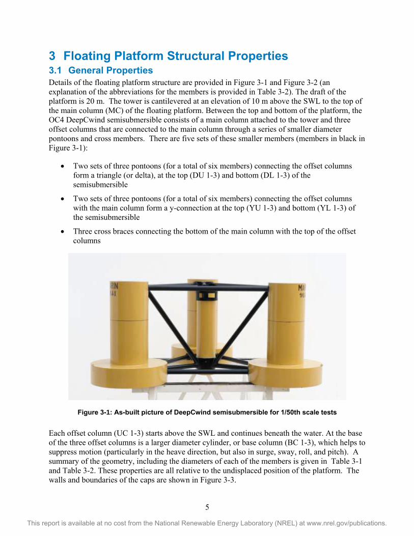
3 Floating Platform Structural Properties 3.1 General Properties Details of the floating platform structure are provided in Figure 3-1 and Figure 3-2 (an explanation of the abbreviations for the members is provided in Table 3-2). The draft of the platform is 20 m. The tower is cantilevered at an elevation of 10 m above the SWL to the top of the main column (MC) of the floating platform. Between the top and bottom of the platform, the OC4 DeepCwind semisubmersible consists of a main column attached to the tower and three offset columns that are connected to the main column through a series of smaller diameter pontoons and cross members. There are five sets of these smaller members (members in black in Figure 3-1):

• Two sets of three pontoons (for a total of six members) connecting the offset columns form a triangle (or delta), at the top (DU 1-3) and bottom (DL 1-3) of the semisubmersible

• Two sets of three pontoons (for a total of six members) connecting the offset columns with the main column form a y-connection at the top (YU 1-3) and bottom (YL 1-3) of the semisubmersible

• Three cross braces connecting the bottom of the main column with the top of the offset columns

Figure 3-1: As-built picture of DeepCwind semisubmersible for 1/50th scale tests

Each offset column (UC 1-3) starts above the SWL and continues beneath the water. At the base of the three offset columns is a larger diameter cylinder, or base column (BC 1-3), which helps to suppress motion (particularly in the heave direction, but also in surge, sway, roll, and pitch). A summary of the geometry, including the diameters of each of the members is given in Table 3-1 and Table 3-2. These properties are all relative to the undisplaced position of the platform. The walls and boundaries of the caps are shown in Figure 3-3.

6


Figure 3-2: Plan (left) and side (right) view of the DeepCwind semisubmersible platform (abbreviations can be found in Table 3-2)

Figure 3-3: Side view of platform walls and caps (abbreviations can be found in Table 3-2)

40.87 m Y

X

DL1, DU1

UC1 BC1

UC2BC2

UC3BC3

DL2, DU2

DL3, DU3

YL2, YU2,CB2

YL1, YU1,CB1

YL3, YU3,CB3

MCY

Z

UC1UC3

BC3 BC1

CB1CB3

DL3

DU3

MC

7


Table 3-1: Floating Platform Geometry

Depth of platform base below SWL (total draft) 20 m Elevation of main column (tower base) above SWL 10 m

Elevation of offset columns above SWL 12 m

Spacing between offset columns 50 m

Length of upper columns 26 m

Length of base columns 6 m

Depth to top of base columns below SWL 14 m

Diameter of main column 6.5 m

Diameter of offset (upper) columns 12 m

Diameter of base columns 24 m

Diameter of pontoons and cross braces 1.6 m

Table 3-2: Member Geometry

Column Name Abbr. Start location (X,Y,Z)

End location (X,Y,Z)

Length (m)

Wall Thick.

(m)

Main Column MC (0, 0,-20) (0, 0,10) 30 0.03

Upper Column 1 UC1 (14.43, 25, -14) (14.43, 25, 12) 26 0.06

Upper Column 2 UC2 (-28.87, 0, -14) (-28.87, 0, 12) 26 0.06

Upper Column 3 UC3 (14.43, -25, -14) (14.43, -25, 12) 26 0.06

Base Column 1 BC1 (14.43, 25, -20) (14.43, 25, -14) 6 0.06

Base Column 2 BC2 (-28.87, 0, -20) (-28.87, 0, -14) 6 0.06

Base Column 3 BC3 (14.43, -25, -20) (14.43, -25, -14) 6 0.06

Delta Pontoon, Upper 1 DU1 (9.20, 22, 10) (-23.67, 3, 10) 38 0.0175

Delta Pontoon, Upper 2 DU2 (-23.67, -3, 10) (9.20, -22, 10) 38 0.0175

Delta Pontoon, Upper 3 DU3 (14.43, -19, 10) (14.43, 19, 10) 38 0.0175

Delta Pontoon, Lower 1 DL1 (4, 19, -17) (-18.47, 6, -17) 26 0.0175

Delta Pontoon, Lower 2 DL2 (-18.47, -6, -17) (4, -19, -17) 26 0.0175

Delta Pontoon, Lower 3 DL3 (14.43, -13, -17) (14.43, 13, -17) 26 0.0175

8


Y Pontoon, Upper 1 YU1 (1.625, 2.815, 10) (11.43, 19.81, 10) 19.62 0.0175

Y Pontoon, Upper 2 YU2 (-3.25, 0, 10) (-22.87, 0, 10) 19.62 0.0175

Y Pontoon, Upper 3 YU3 (1.625, -2.815, 10) (11.43, -19.81, 10) 19.62 0.0175

Y Pontoon, Lower 1 YL1 (1.625, 2.815, -17) (8.4, 14.6, -17) 13.62 0.0175

Y Pontoon, Lower 2 YL2 (-3.25, 0, -17) (-16.87, 0, -17) 13.62 0.0175

Y Pontoon, Lower 3 YL3 (1.625, -2.815, -17) (8.4, -14.6, -17) 13.62 0.0175

Cross Brace 1 CB1 (1.625, 2.815, -16.2) (11.43, 19.81, 9.13) 32.04 0.0175

Cross Brace 2 CB2 (-3.25, 0, -16.2) (-22.87, 0, 9.13) 32.04 0.0175

Cross Brace 3 CB3 (1.625, -2.815, -16.2) (11.43, -19.81, 9.13) 32.04 0.0175

Upper Col. Top Cap UCTC 0.06

Upper Col. Bottom Cap UCBC 0.06

Base Col. Top Cap BCTC 0.06

Base Col. Bottom Cap BCBC 0.06

Main Col. bottom cap MCBC 0.03

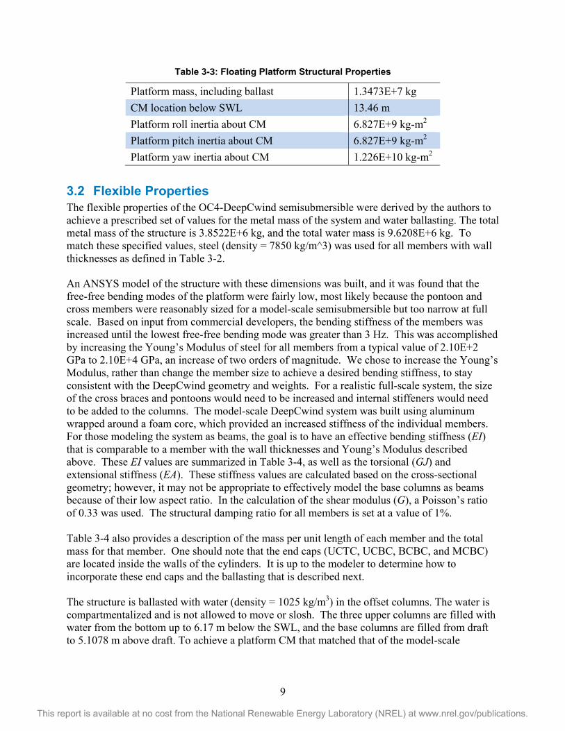
The mass, including ballast, of the floating platform is 1.3473E+7 kg. This mass was calculated such that the combined weight of the rotor-nacelle assembly, tower, and floating platform, plus the weight of the mooring system (not including the small portion resting on the seafloor) in water balances with the buoyancy (i.e. weight of the displaced fluid) of the undisplaced platform in still water. The CM of the floating platform, which includes everything except the tower, rotor-nacelle assembly, and moorings, is located at 13.46 m along the platform centerline below the SWL. This value was set so that the overall system CM matched that of the scale-model DeepCwind system. The roll and pitch inertias of the floating platform about its CM are both 6.827E+9 kg-m2 about the platform x-axis and y-axis respectively, and the yaw inertia of the floating platform about its centerline is 1.226E+10 kg-m2.

Table 3-3 summarizes the undisplaced platform properties discussed in this section.

9


Table 3-3: Floating Platform Structural Properties

Platform mass, including ballast 1.3473E+7 kg CM location below SWL 13.46 m Platform roll inertia about CM 6.827E+9 kg-m2 Platform pitch inertia about CM 6.827E+9 kg-m2 Platform yaw inertia about CM 1.226E+10 kg-m2

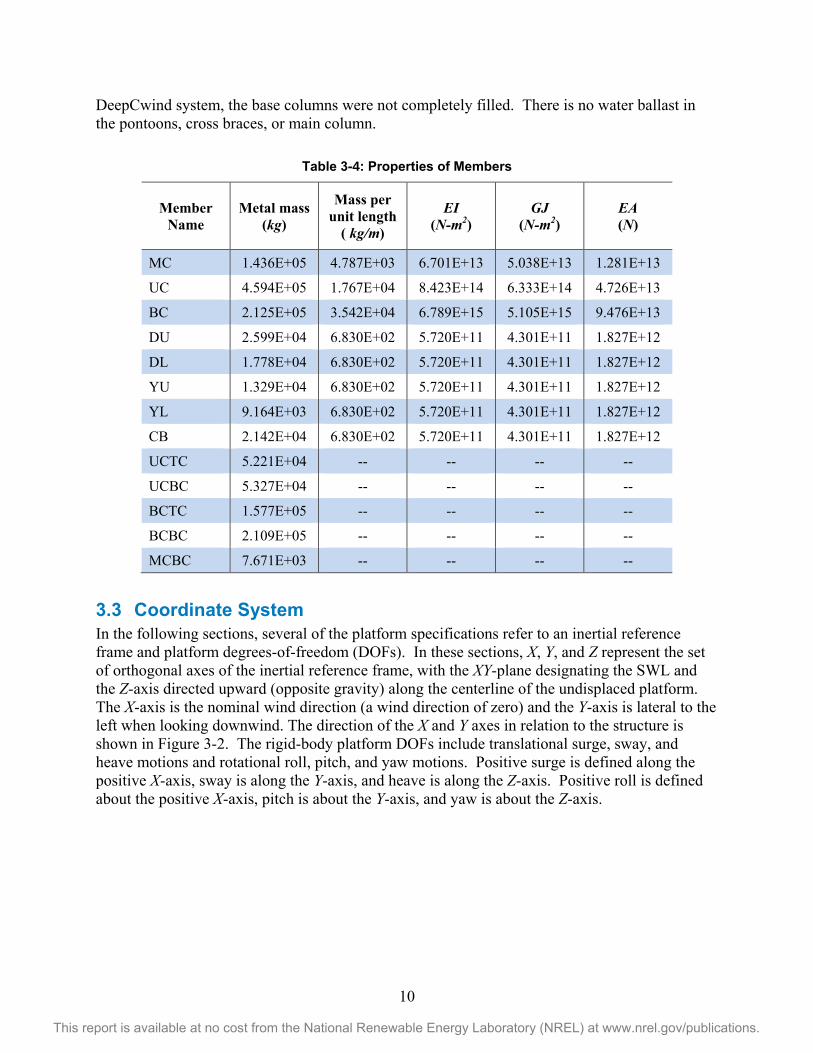
3.2 Flexible Properties The flexible properties of the OC4-DeepCwind semisubmersible were derived by the authors to achieve a prescribed set of values for the metal mass of the system and water ballasting. The total metal mass of the structure is 3.8522E+6 kg, and the total water mass is 9.6208E+6 kg. To match these specified values, steel (density = 7850 kg/m^3) was used for all members with wall thicknesses as defined in Table 3-2. An ANSYS model of the structure with these dimensions was built, and it was found that the free-free bending modes of the platform were fairly low, most likely because the pontoon and cross members were reasonably sized for a model-scale semisubmersible but too narrow at full scale. Based on input from commercial developers, the bending stiffness of the members was increased until the lowest free-free bending mode was greater than 3 Hz. This was accomplished by increasing the Young’s Modulus of steel for all members from a typical value of 2.10E+2 GPa to 2.10E+4 GPa, an increase of two orders of magnitude. We chose to increase the Young’s Modulus, rather than change the member size to achieve a desired bending stiffness, to stay consistent with the DeepCwind geometry and weights. For a realistic full-scale system, the size of the cross braces and pontoons would need to be increased and internal stiffeners would need to be added to the columns. The model-scale DeepCwind system was built using aluminum wrapped around a foam core, which provided an increased stiffness of the individual members. For those modeling the system as beams, the goal is to have an effective bending stiffness (EI) that is comparable to a member with the wall thicknesses and Young’s Modulus described above. These EI values are summarized in Table 3-4, as well as the torsional (GJ) and extensional stiffness (EA). These stiffness values are calculated based on the cross-sectional geometry; however, it may not be appropriate to effectively model the base columns as beams because of their low aspect ratio. In the calculation of the shear modulus (G), a Poisson’s ratio of 0.33 was used. The structural damping ratio for all members is set at a value of 1%. Table 3-4 also provides a description of the mass per unit length of each member and the total mass for that member. One should note that the end caps (UCTC, UCBC, BCBC, and MCBC) are located inside the walls of the cylinders. It is up to the modeler to determine how to incorporate these end caps and the ballasting that is described next. The structure is ballasted with water (density = 1025 kg/m3) in the offset columns. The water is compartmentalized and is not allowed to move or slosh. The three upper columns are filled with water from the bottom up to 6.17 m below the SWL, and the base columns are filled from draft to 5.1078 m above draft. To achieve a platform CM that matched that of the model-scale

10


DeepCwind system, the base columns were not completely filled. There is no water ballast in the pontoons, cross braces, or main column.

Table 3-4: Properties of Members

Member Name

Metal mass (kg)

Mass per unit length

( kg/m)

EI (N-m2)

GJ (N-m2)

EA (N)

MC 1.436E+05 4.787E+03 6.701E+13 5.038E+13 1.281E+13

UC 4.594E+05 1.767E+04 8.423E+14 6.333E+14 4.726E+13

BC 2.125E+05 3.542E+04 6.789E+15 5.105E+15 9.476E+13

DU 2.599E+04 6.830E+02 5.720E+11 4.301E+11 1.827E+12

DL 1.778E+04 6.830E+02 5.720E+11 4.301E+11 1.827E+12

YU 1.329E+04 6.830E+02 5.720E+11 4.301E+11 1.827E+12

YL 9.164E+03 6.830E+02 5.720E+11 4.301E+11 1.827E+12

CB 2.142E+04 6.830E+02 5.720E+11 4.301E+11 1.827E+12

UCTC 5.221E+04 -- -- -- --

UCBC 5.327E+04 -- -- -- --

BCTC 1.577E+05 -- -- -- --

BCBC 2.109E+05 -- -- -- --

MCBC 7.671E+03 -- -- -- --

3.3 Coordinate System In the following sections, several of the platform specifications refer to an inertial reference frame and platform degrees-of-freedom (DOFs). In these sections, X, Y, and Z represent the set of orthogonal axes of the inertial reference frame, with the XY-plane designating the SWL and the Z-axis directed upward (opposite gravity) along the centerline of the undisplaced platform. The X-axis is the nominal wind direction (a wind direction of zero) and the Y-axis is lateral to the left when looking downwind. The direction of the X and Y axes in relation to the structure is shown in Figure 3-2. The rigid-body platform DOFs include translational surge, sway, and heave motions and rotational roll, pitch, and yaw motions. Positive surge is defined along the positive X-axis, sway is along the Y-axis, and heave is along the Z-axis. Positive roll is defined about the positive X-axis, pitch is about the Y-axis, and yaw is about the Z-axis.

11


4 Floating Platform Hydrodynamic Properties 4.1 Overview Hydrodynamic loads on offshore wind systems include contributions from linear hydrostatics, linear excitation from incident waves, linear radiation from outgoing waves (generated by platform motion), and nonlinear effects. Depending on the code being used, each of these components may be treated in a different manner. Some codes may use a potential theory-based approach for modeling the hydrodynamics, some may use Morison’s equation, and some may use a combination of the two. Depending on which approach is used, only some of the sections in this chapter are applicable (see Table 4-1).

Table 4-1: Applicable Sections for Hydrodynamics Modeling Approaches

Applicable Sections Hydrodynamics modeling approach

Section 4.2 Hydrostatics

Section 4.3.2 Potential flow

theory

Section 4.3.3 Morison’s Eq.

Section 4.4 Additional damping

Potential flow theory only X X X

Morison’s equation only X X

Potential theory and Morison’s equation

X X X

X = Needed if Morison-only model neglects buoyancy

4.2 Hydrostatics If using a code with either a potential-flow theory or Morison-based approach that neglects buoyancy, one must ensure that the hydrostatic component described in this section is included. The total load on the floating platform from linear hydrostatics, Hydrostatic

iF , is

( )Hydrostatic Hydrostatici 0 i3 ij jF q gV C qρ δ= − , (4-1)

where ρ is the water density, g is the gravitational acceleration constant, V0 is the displaced volume of fluid when the platform is in its undisplaced position, δi3 is the (i,3) component of the Kronecker-Delta function (i.e. identity matrix), Hydrostatic

ijC is the (i,j) component of the linear hydrostatic-restoring matrix from the effects of water-plane area at the center of buoyancy (COB), and jq is the jth platform DOF. (Without the subscript, q represents the set of platform DOFs. Hydrostatic

iF depends on q as indicated.) In Eq. (4-1), subscripts i and j range from 1 to 6; one for each platform DOF (1 = surge, 2 = sway, 3 = heave, 4 = roll, 5 = pitch, 6 = yaw).

12


Einstein notation is used here, in which it is implied that when the same subscript appears in multiple variables in a single term, there is a sum of all of the possible terms. The loads are positive in the direction of positive motion of DOF i. Equation (4-1) does not include the restoring effects of body weight (i.e. gravitational restoring). Instead, the gravitational restoring is assumed to be included within the structural dynamics models. The first of the terms on the right-hand side of Eq. (4-1) represents the buoyancy force from Archimedes’ principle; that is, it is the force directed vertically upward and equal to the weight of the displaced fluid when the platform is in its undisplaced position. This term is nonzero only for the vertical heave-displacement DOF of the support platform (DOF i = 3) because the COB lies on the centerline of the undeflected tower. The second of the terms on the right-hand side of Eq. (4-1) represents the change in the hydrostatic force and moment as the platform is displaced. The formulation for Hydrostatic

ijC in terms of a platform’s water-plane shape, displaced volume, and COB location is given in (Jonkman 2007). The water density is chosen to be 1,025 kg/m3. From the external geometry of the floating platform, then, ρgV0 and Hydrostatic

ijC were calculated to be:

𝜌𝑔𝑉0 =1.3989e8 N (4-2)

and

Hydrostaticij

0 0 0 0 0 00 0 0 0 0 00 0 3.836e6 N m 0 0 0

C0 0 0 -3.776e8 Nm rad 0 00 0 0 0 -3.776e8 Nm rad 00 0 0 0 0 0

=

(4-3)

4.3 Hydrodynamics The hydrodynamic loads―those associated with excitation from incident waves, radiation of outgoing waves from platform motion, added mass effects, and viscous forces―depend on a variety of factors, all of which will be discussed next. In this section, we demonstrate several methods to implement the hydrodynamic forces. The choice of method will depend on the hydrodynamics capabilities of the modeling tool being used. The scope of this document is focused on wave forces associated with radiation damping, added-mass, wave-excitation loads, and loads arising from flow separation. Hence, the second-order Quadratic Transfer Functions (QTFs) will not be defined here, but these effects could be considered in models that are capable. 4.3.1 Dimensionless Numbers for Flow/Structure Interaction For a floating platform interacting with surface waves, different formulations for the hydrodynamic loads apply to separated and nonseparated flows. For cylinders, the proper

13


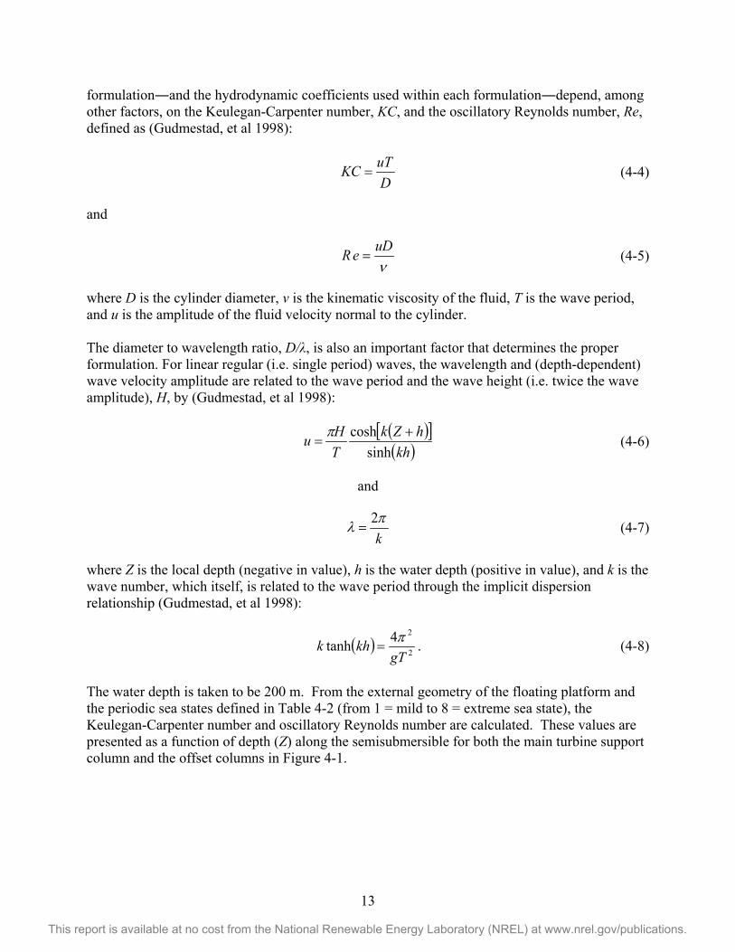
formulation―and the hydrodynamic coefficients used within each formulation―depend, among other factors, on the Keulegan-Carpenter number, KC, and the oscillatory Reynolds number, Re, defined as (Gudmestad, et al 1998):

DuTKC = (4-4)

and

νuDeR = (4-5)

where D is the cylinder diameter, ν is the kinematic viscosity of the fluid, T is the wave period, and u is the amplitude of the fluid velocity normal to the cylinder. The diameter to wavelength ratio, D/λ, is also an important factor that determines the proper formulation. For linear regular (i.e. single period) waves, the wavelength and (depth-dependent) wave velocity amplitude are related to the wave period and the wave height (i.e. twice the wave amplitude), H, by (Gudmestad, et al 1998):

( )[ ]( )kh

hZkTHu

sinhcosh +

=π

(4-6)

and

kπλ 2

= (4-7)

where Z is the local depth (negative in value), h is the water depth (positive in value), and k is the wave number, which itself, is related to the wave period through the implicit dispersion relationship (Gudmestad, et al 1998):

( ) 2

24tanhgT

khk π= . (4-8)

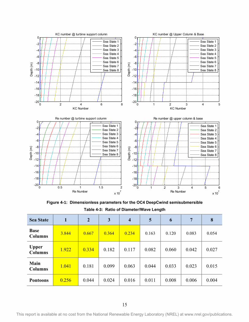
The water depth is taken to be 200 m. From the external geometry of the floating platform and the periodic sea states defined in Table 4-2 (from 1 = mild to 8 = extreme sea state), the Keulegan-Carpenter number and oscillatory Reynolds number are calculated. These values are presented as a function of depth (Z) along the semisubmersible for both the main turbine support column and the offset columns in Figure 4-1.

14


Table 4-2: Periodic Sea State Definitions

Sea State T (s) H (m)

1 2.0 0.09

2 4.8 0.67

3 6.5 1.40

4 8.1 2.44

5 9.7 3.66

6 11.3 5.49

7 13.6 9.14

8 17.0 15.24

The upper and lower plots in Figure 4-1 show that, for the OC4-DeepCwind semisubmersible, the KC and oscillatory Re numbers grow with increasing severity in the wave conditions and decrease with depth (due to a decrease in the fluid velocity) for a constant-diameter section. The jump in values in the offset column plots occur at the point where the column diameter changes from that of the base column to the upper column. For the pontoons, the cylinder axis might not lie in the same plane as the two-dimensional flow; therefore, a range of values is possible based on the alignment of the flow direction with the cylinder axis.

Flow separation becomes important when the KC number exceeds 2. For values lower than 2, potential-flow theory applies. Consequently, potential-flow theory applies for all of the large components of the semisubmersible in all but the most extreme wave conditions (sea states 6 – 8), where separation will occur along the main column and upper portions of the offset columns. For the pontoons and cross members, flow separation occurs in sea states 5 – 8.

Additionally, the diameter to wavelength ratio is calculated for the main and offset columns as well as the pontoons. This result is shown in Table 4-3. Table 4-3 shows that for the OC4-DeepCwind semisubmersible, the diameter to wavelength ratio decreases with increasing severity of the wave conditions and is lowest for the smaller diameter members, such as the pontoons. Diffraction effects are important when this ratio exceeds 0.2 and are unimportant for smaller ratios. In Table 4-3, the cases where wave diffraction is important have been highlighted. These cases mainly include the lowest sea states, where the hydrodynamic loads are small anyway, but also include half of the sea state states for the large diameter base of the offset columns.

15


Figure 4-1: Dimensionless parameters for the OC4 DeepCwind semisubmersible

Table 4-3: Ratio of Diameter/Wave Length

Sea State 1 2 3 4 5 6 7 8

Base Columns 3.844 0.667 0.364 0.234 0.163 0.120 0.083 0.054

Upper Columns 1.922 0.334 0.182 0.117 0.082 0.060 0.042 0.027

Main Columns 1.041 0.181 0.099 0.063 0.044 0.033 0.023 0.015

Pontoons 0.256 0.044 0.024 0.016 0.011 0.008 0.006 0.004

0 2 4 6 8-20

-18

-16

-14

-12

-10

-8

-6

-4

-2

0KC number @ turbine support column

KC Number

Dep

th (m

)

Sea State 1Sea State 2Sea State 3Sea State 4Sea State 5Sea State 6Sea State 7Sea State 8

0 1 2 3 4 5-20

-18

-16

-14

-12

-10

-8

-6

-4

-2

0KC number @ Upper Column & Base

KC Number

Dep

th (m

)


0 0.5 1 1.5 2

x 107

-20

-18

-16

-14

-12

-10

-8

-6

-4

-2

0Re number @ turbine support column

Re Number

Dep

th (m

)


0 1 2 3 4 5 6

x 107

-20

-18

-16

-14

-12

-10

-8

-6

-4

-2

0Re number @ upper column & base

Re Number

Dep

th (m

)


16


4.3.2 Potential-Flow Theory In view of the validity of potential-flow theory across many conditions, the linear potential-flow problem was solved using WAMIT (Lee and Newman 2006), and the output from this analysis was shared with the participants. WAMIT uses a three-dimensional numerical-panel method in the frequency domain to solve the linearized potential-flow hydrodynamic radiation and diffraction problems for the interaction of surface waves with offshore platforms of arbitrary geometry. The solution to the radiation problem, which considers the hydrodynamic loads on the platform associated with oscillation of the platform in its various modes of motion (which radiate outgoing waves), is given in terms of oscillation-frequency-dependent hydrodynamic added-mass and damping matrices, Aij and Bij respectively. The solution to the diffraction problem, which considers the hydrodynamic loads on the platform associated with excitation from incident waves, is given in terms of the wave-frequency and direction-dependent hydrodynamic wave-excitation vector, Xi. Whereas Aij and Bij are real-valued, Xi is complex-valued, with the magnitude determining the load normalized per unit wave amplitude and the phase determining the lag between the wave elevation and load. The subscripts here are consistent with those of

HydrostaticijC discussed earlier and, as before, the loads are positive in the direction of positive

motion. More information on potential-flow theory as it relates to floating platforms can be found in (Jonkman 2007). In WAMIT, the OC4-DeepCwind semisubmersible was modeled with one geometric plane of symmetry using a high-order representation of the geometry from a MultiSurf surface file. In the high-order representation of a WAMIT geometric description, the velocity potential on the body is represented by B-splines in a continuous manner. The model employed an average panel size of 2 m. To further improve the accuracy of the WAMIT results, options were selected to integrate the logarithmic singularity analytically, solve the linear system of equations using a direct solver, and remove the effects of irregular frequencies by manually paneling the free surface. These settings were beneficial because of the requirement of high-frequency output for time-domain analysis. The semisubmersible was analyzed in its undisplaced position (consistent with linear theory) and with finite water depth (200 m). The magnitude and phase of the hydrodynamic wave-excitation vector from the linear diffraction problem are shown as a function of wave frequency in Figure 4-2 for incident waves propagating along the positive X-axis. For these waves, the loads in the direction of the sway (Mode 2), roll (Mode 4), and yaw (Mode 6) DOFs are zero because the wave forces lie within the XZ platform plane. The hydrodynamic added mass and damping matrices for the six DOFs are shown as a function of oscillation frequency in Figure 4-3. Only the upper triangular matrix elements are shown because the hydrodynamic added-mass and damping matrices are symmetric in the absence of forward motion. Also, because of the semisubmersible’s symmetries, the surge-surge elements of the frequency-dependent added-mass and damping matrices, A11 and B11, are identical to the sway-sway elements, A22 and B22. Likewise, the roll-roll elements, A44 and B44, are identical to the pitch-pitch elements, A55 and B55. This behavior exists because the OC4-DeepCwind semisubmersible has the same response at 0°, 120°, and 240° wave headings, (see Figure 4-4) which means that the X and Y responses must also be the same. Other matrix elements not shown are zero-valued. The zero and infinite-frequency limits of all elements of the damping

17


matrix are zero, as required by potential theory, and peak at intermediate frequencies. The infinite-frequency added-mass matrix, A∞, is defined as:

2

2

2

6.49E+6 kg 0 0 0 -85.10E+6 kg m 00 6.49E+6 kg 0 85.10E+6 kg m 0 00 0 14.70E+6 kg 0 0 00 85.10E+6 kg m 0 7.21E+9 kg m 0 0

-85.10E+6 kg m 0 0 0 7.21E+9 kg m 00 0 0 0 0 4.87E+9 kg m

A∞

⋅ ⋅

= ⋅ ⋅ ⋅ ⋅ ⋅

Figure 4-2: Hydrodynamic wave excitation per unit amplitude for the OC4 semisubmersible for 0°

wave heading

18


Figure 4-3: Hydrodynamic added mass and damping for the OC4-DeepCwind semisubmersible

19


Figure 4-4: Simplified plan footprint of the OC4 semisubmersible

The linear memory effect is captured within time-domain hydrodynamics models through the time-convolution of the radiation impulse-response functions (i.e. the wave-radiation-retardation kernel), Kij, with the platform velocities. The memory effect captures the hydrodynamic load on the platform persisting from the outgoing free-surface waves (which induce a pressure field within the fluid domain) radiated away by platform motion. The radiation impulse-response functions can be found from the cosine transform of the frequency-dependent hydrodynamic damping matrix. The results of this computation, as performed within WAMIT’s frequency-to-time (F2T) conversion utility, are shown in Figure 4-5. As before, only the upper triangular matrix elements of the symmetric Kij matrix are shown, and because of the semisubmersible’s symmetry, the surge-surge elements, K11, are identical to the sway-sway elements, K22, and the roll-roll elements, K44, are identical to the pitch-pitch elements, K55. Most of the response and linear radiation damping decays to zero after about 40 seconds, even for the force-translation modes that may not be negligible. For more information on radiation theory, see (Jonkman 2007).

The second-order potential-flow solution, which includes mean-drift, slow-drift, and sum-frequency excitation, and higher-order solutions, were not solved.

20


Figure 4-5: Radiation impulse-response functions for the OC4-DeepCwind semisubmersible

4.3.3 Morison’s Equation In severe sea conditions, the hydrodynamic loads from linear potential-flow theory must be augmented with the loads brought about by flow separation. Moreover, many wind turbine dynamics codes cannot model hydrodynamics per linear potential-flow theory and use only a Morison-based approach for all sea conditions. To address these situations, a simplified hydrodynamics model using Morison’s formulation is presented next. The popular hydrodynamic formulation used in the analysis of fixed-bottom support structures for offshore wind turbines, Morison’s formulation, is applicable for calculating the hydrodynamic loads on cylindrical structures when (1) the effects of diffraction can be simplified with the long wavelength approximation, (2) radiation damping is negligible, and (3) flow separation may occur. The relative form of Morison’s equation accounts for wave loading from incident-wave-induced excitation, radiation-induced added mass, and flow-separation-induced viscous drag. In the next two sections we review the representation of Morison’s equation in flow transverse to the structure and for a heave plate.

21


4.3.3.1 Transverse Flow For a cylinder in steady, transverse flow, the wave forces per unit length on the cylinder with velocity q can be expressed as:

2 21 ( ) (1 )

2 4 4d a aD DF C D u q u q C u C qπ πρ ρ ρ= − − + + − (4-9)

where ρ is the fluid density, D is the diameter of the cylinder, Cd is the drag coefficient, and Ca is the added mass coefficient. Equation (4-9) is comprised of a quadratic drag term, the fluid-inertia excitation force, and the added-mass term. In addition, some Morison-based software programs will account for the dynamic pressure caused by the varying water elevation. From the discussion in Section 4.3.1, Morison’s equation is a reasonable approximation for the OC4-DeepCwind semisubmersible in most wave conditions because (1) diffraction effects can be approximated by long wavelength theory in moderate to severe sea states, (2) radiation damping in most modes is small, and (3) flow separation will occur in severe sea states along the upper column regions of the semisubmersible. In the next sections, we demonstrate the methodology to obtain the drag coefficient Cd and added-mass coefficient Ca in Equation (4-9).

Added Mass The added-mass coefficient Ca to be used in Equation (4-9) was selected such that CaρV equaled the zero-frequency limit of A11 in the surge direction from the potential-flow solution (Figure 4-3). This equivalency was based on the assumption that Ca is independent of water depth and the motion is of low frequency. By this equivalency, an initial estimate for the added mass coefficient for each member of the DeepCwind semisubmersible was 0.63. This value should be used for all members in all platform degrees of freedom, with the exception of heave, which will be addressed below. To verify the cross-flow added mass coefficient Ca = 0.63, three models were assembled in OrcaFlex (a commercial modeling tool for offshore structures) using the platform geometric properties outlined in Table 3-1 through Table 3-3, each with different representations of the added mass:

• Model 1: models the added mass force contribution using Morison’s equation • Model 2: includes only the WAMIT added mass coefficients • Model 3: no added mass is modeled

Model 3 was constructed purely for curiosity measures to quantify the significance of added mass on the system. The comparison was performed in OrcaFlex because this software allows for input of the WAMIT solution and provides an opportunity to attach Morison added-mass elements discretely along the various column members and cross braces, thus allowing each discrete component to be modeled with unique hydrodynamic properties. Each model was prescribed an impulse force to compel the platform to freely oscillate. By comparing the motion of Model 1 with Model 2, it was decided that Ca = 0.63 is a satisfactory coefficient to use when modeling the cross-flow column added mass using Morison’s equation.

22


Viscous Drag With the added mass coefficient, Ca, selected, we can now focus on determining the drag coefficient dC for Equation (4-9). For a cylinder in steady, transverse flow, the drag coefficient is determined based on the Reynold’s number using the relationship provided in Figure 4-6 (Catalano, et al 2003). In this figure, the Re values for each of the semisubmersible’s members in various sea states are plotted using markers. As shown, the drag force can vary greatly across the flow regimes the system is likely to encounter, and therefore an average dC value is calculated for each member, as outlined in Appendix I and summarized in Table 4-4. Note that these values are derived for the full-scale system and associated Re values. A different set of

dC values would be chosen to match the drag characteristics of the DeepCwind tank tests, which were performed at model scale and therefore encompassed very different Re values. The KC number was not considered in this calculation.

Figure 4-6: Distribution of the drag coefficient as a function of the Re number

Table 4-4: Mean Cd Values Across All Sea States for the Full-Scale OC4 Semisubmersible

Column D=1.6 m D=6.5 m D=12 m D=24 m

Cd 0.63 0.56 0.61 0.68

4.3.3.2 Heave Plate Unlike a cylinder in cross-flow, the force on a heave plate does not scale proportionally to the displaced fluid (because the heave plate displaces little volume). The three base columns are

23


considered as heave plates. The hydrodynamic heave force for a heave plate is formulated using this modified Morison’s equation (to include dynamic pressure) as given below:

𝐹𝑧 = 12𝜌𝐶𝑑𝑧𝐴𝐶|𝑤 − �̇�3|(𝑤 − �̇�3) + 𝜌𝐶𝑎𝑧𝑉𝑅(�̇� − �̈�3) +

𝜋4𝐷ℎ2𝑝𝑏 −

𝜋4

(𝐷ℎ2 − 𝐷𝑐2)𝑝𝑡 (4-10)

where 𝐶𝑑𝑧 is the drag coefficient in the heave direction, 𝐴𝐶 is the cross-sectional area of the heave-plate in the Z-direction, 𝑤 is the vertical wave particle velocity, �̇�3 is the heave velocity of the heave-plate, 𝐶𝑎𝑧 is the added mass coefficient in the heave direction, 𝑉𝑅 is the reference volume, �̇� is the vertical wave particle acceleration, �̈�3 is the heave acceleration of the heave-plate, 𝐷ℎ is the diameter of the heave-plate, 𝐷𝑐 is the diameter of the upper column (which is placed on top of the heave-plate), and 𝑝𝑏 and 𝑝𝑡 are the dynamic pressure acting at the bottom and top faces of the heave-plate. In equation (4-10), the first term corresponds to the drag force in the heave direction, the second term corresponds to the combined fluid acceleration (scattering) and added mass force, and the last two terms correspond to the Froude-Krylov force expressed in terms of dynamic pressure. Please note that the viscous drag, fluid-acceleration, and added mass terms are shown for an entire heave-plate collectively, but could also be expressed with separate forces on the bottom and top faces.

Added Mass A separate added mass coefficient for the heave direction must be used to properly model the column-base added mass. The following relationship can be used to find the added mass coefficient, Caz, in the heave direction:

33 (0)az

R

ACVρ

= (4-11)

where 𝐴33(0) is the zero-frequency limit added mass in the heave direction obtained from WAMIT (which can be found in Figure 4-3). Equation (4-11) is valid for the entire structure. To consider only one of the three columns, the value for 𝐴33(0) would need to be divided by three, and the reference volume would only be for that one column rather than the entire structure. This assumes that the contribution of the cross braces and main column to the heave added mass is negligible. One can use any appropriate combination of 𝐶𝑎𝑧 and 𝑉𝑅 that produces the correct added mass. For example, if 𝐶𝑎𝑧 is chosen as 1.0, then for one column: 𝑉𝑅 = 𝐴33(0)/3

𝜌= 4.88E+3 m3.

Similarly, if 𝑉𝑅 is chosen as 𝑉𝑅 = 43𝜋𝑟3, where 𝑟 is the heave plate radius, then 𝐶𝑎𝑧 = 𝐴33(0)/3

43𝜋𝜌𝑟

3 =

0.67 for one column.

Viscous Drag As was true for the added-mass coefficient, the heave plates require a separate drag coefficient for the heave direction. Assuming the heave plate emulates a flat plate with flow normal to the face, a value of Cdz = 4.8 is selected. This value was found by matching a coupled

24


FAST+OrcaFlex simulation with DeepCwind tank-test data in the heave direction. In this situation—due to sharp corners—the drag coefficient is no longer strongly dependent on Re number and will be the same for a full-scale or model-scale system, which allows us to derive the value for our full-scale system through comparison to the tank-test data.

4.3.4 Quadratic Drag for Other Models For codes that model potential flow without Morison elements, extra damping is needed to accurately represent the damping in a real system. To determine the amount of additional damping required, free-decay simulations of the semisubmersible using linear potential-flow theory were executed then compared to simulations using a combination of potential-flow theory and the viscous term in Morison’s equation. Each model was constructed in FAST and, as needed, coupled to OrcaFlex (Jonkman and Buhl 2005). For the models not representing viscous elements discretely, i.e. those omitting the viscous component in Equation (4-9), additional quadratic drag was added to the model on top of the potential-flow contribution. This drag is implemented according to the following equation:

( )Additional Drag quad

i ij j jF q B q q= − , (4-12) where quad

ijB is the (i,j) component of the additional quadratic drag matrix, and jq is the first time derivative of the jth platform DOF. The quantities labeled as quad

iiB in Equation (4-12) represent the required quadratic viscous drag coefficient needed to match a simulation using Equation (4-12) against a simulation using discrete Morison viscous drag elements. The off-diagonal elements of matrix quad

ijB are neglected.

Table 4-5: Quadratic Drag Coefficients for the FAST Model

Surge Ns2/m2

Sway Ns2/m2

Heave Ns2/m2

Roll Nms2/rad2

Pitch Nms2/rad2

Yaw Nms2/rad2

quadiiB * 3.95E+5 3.95E+5 3.88E+6 3.70E+10 3.70E+10 4.08E+9

25


4.4 Summary Table 4-6 summarizes the hydrodynamic properties (except the linear potential-flow solution) that were discussed in this section.

Table 4-6: Floating Platform Hydrodynamic Properties

Water density (𝜌) 1025 kg/m3 Water depth (h) 200 m Displaced water in undisplaced position (𝑉0) 13917 m3 Center of buoyancy below SWL 13.15 m

Buoyancy force in undisplaced position (𝜌𝑔𝑉0) 1.3989E+8 N

Hydrostatic restoring in heave (𝐶33𝐻𝑦𝑑𝑟𝑜𝑠𝑡𝑎𝑡𝑖𝑐) 3.836E+06 N/m

Hydrostatic restoring in roll (𝐶44𝐻𝑦𝑑𝑟𝑜𝑠𝑡𝑎𝑡𝑖𝑐) -3.776E+08 N-m/rad

Hydrostatic restoring in pitch (𝐶55𝐻𝑦𝑑𝑟𝑜𝑠𝑡𝑎𝑡𝑖𝑐) -3.776E+08 N-m/rad

Added-mass coefficient (Ca ) for all members 0.63

Added-mass coefficient (Caz ) for base column in z-direction

1.0

Drag coefficient (Cd ) for main column 0.56

Drag coefficient (Cd ) for upper columns 0.61

Drag coefficient (Cd ) for base columns 0.68

Drag coefficient (Cd ) for pontoons and cross members 0.63

Drag coefficient (Cdz ) for base columns in z-direction 4.8

Additional quadratic drag in surge (𝐵11𝑞𝑢𝑎𝑑) 3.95E+5 Ns2/m2

Additional quadratic drag in sway (𝐵22𝑞𝑢𝑎𝑑) 3.95E+5 Ns2/m2

Additional quadratic drag in heave (𝐵33𝑞𝑢𝑎𝑑) 3.88E+6 Ns2/m2

Additional quadratic drag in roll (𝐵44𝑞𝑢𝑎𝑑) 3.70E+10 Nms2/rad2

Additional quadratic drag in pitch (𝐵55𝑞𝑢𝑎𝑑) 3.70E+10 Nms2/rad2

Additional quadratic drag in yaw (𝐵66𝑞𝑢𝑎𝑑) 4.08E+9 Nms2/rad2

26


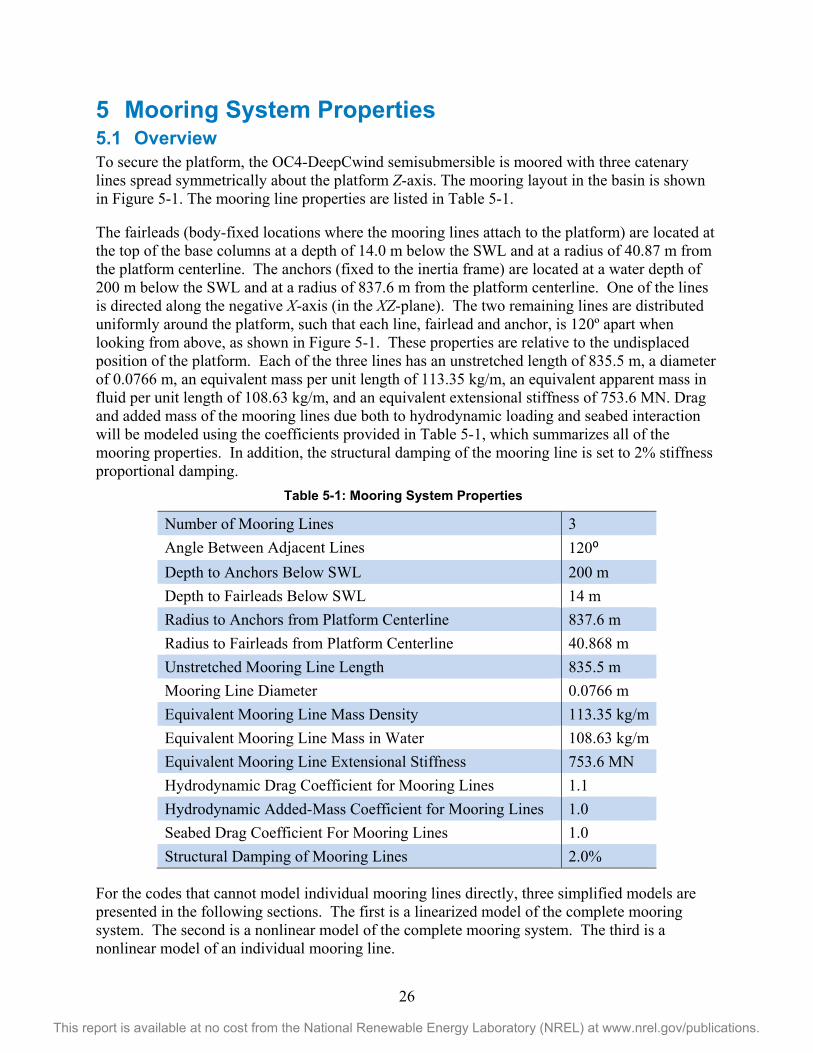
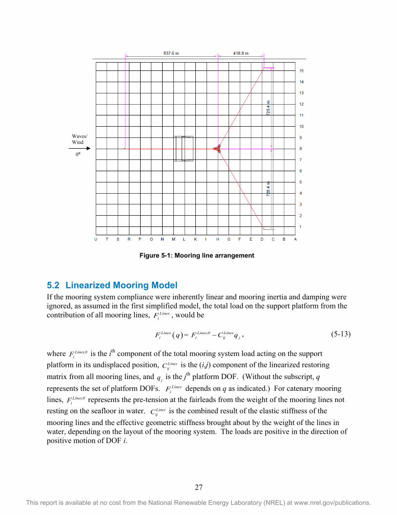
5 Mooring System Properties 5.1 Overview To secure the platform, the OC4-DeepCwind semisubmersible is moored with three catenary lines spread symmetrically about the platform Z-axis. The mooring layout in the basin is shown in Figure 5-1. The mooring line properties are listed in Table 5-1. The fairleads (body-fixed locations where the mooring lines attach to the platform) are located at the top of the base columns at a depth of 14.0 m below the SWL and at a radius of 40.87 m from the platform centerline. The anchors (fixed to the inertia frame) are located at a water depth of 200 m below the SWL and at a radius of 837.6 m from the platform centerline. One of the lines is directed along the negative X-axis (in the XZ-plane). The two remaining lines are distributed uniformly around the platform, such that each line, fairlead and anchor, is 120º apart when looking from above, as shown in Figure 5-1. These properties are relative to the undisplaced position of the platform. Each of the three lines has an unstretched length of 835.5 m, a diameter of 0.0766 m, an equivalent mass per unit length of 113.35 kg/m, an equivalent apparent mass in fluid per unit length of 108.63 kg/m, and an equivalent extensional stiffness of 753.6 MN. Drag and added mass of the mooring lines due both to hydrodynamic loading and seabed interaction will be modeled using the coefficients provided in Table 5-1, which summarizes all of the mooring properties. In addition, the structural damping of the mooring line is set to 2% stiffness proportional damping.

Table 5-1: Mooring System Properties

Number of Mooring Lines 3 Angle Between Adjacent Lines 120⁰ Depth to Anchors Below SWL 200 m Depth to Fairleads Below SWL 14 m Radius to Anchors from Platform Centerline 837.6 m Radius to Fairleads from Platform Centerline 40.868 m Unstretched Mooring Line Length 835.5 m Mooring Line Diameter 0.0766 m Equivalent Mooring Line Mass Density 113.35 kg/m Equivalent Mooring Line Mass in Water 108.63 kg/m Equivalent Mooring Line Extensional Stiffness 753.6 MN Hydrodynamic Drag Coefficient for Mooring Lines 1.1 Hydrodynamic Added-Mass Coefficient for Mooring Lines 1.0 Seabed Drag Coefficient For Mooring Lines 1.0 Structural Damping of Mooring Lines 2.0%

For the codes that cannot model individual mooring lines directly, three simplified models are presented in the following sections. The first is a linearized model of the complete mooring system. The second is a nonlinear model of the complete mooring system. The third is a nonlinear model of an individual mooring line.

27


Figure 5-1: Mooring line arrangement

5.2 Linearized Mooring Model If the mooring system compliance were inherently linear and mooring inertia and damping were ignored, as assumed in the first simplified model, the total load on the support platform from the contribution of all mooring lines, Lines

iF , would be

( )Lines Lines,0 Linesi i ij jF q = F C q− , (5-13)

where Lines,0iF is the ith component of the total mooring system load acting on the support

platform in its undisplaced position, LinesijC is the (i,j) component of the linearized restoring

matrix from all mooring lines, and jq is the jth platform DOF. (Without the subscript, q represents the set of platform DOFs. Lines

iF depends on q as indicated.) For catenary mooring lines, Lines,0

iF represents the pre-tension at the fairleads from the weight of the mooring lines not resting on the seafloor in water. Lines

ijC is the combined result of the elastic stiffness of the mooring lines and the effective geometric stiffness brought about by the weight of the lines in water, depending on the layout of the mooring system. The loads are positive in the direction of positive motion of DOF i.

Waves/ Wind 0⁰

28


For the mooring system considered here, Lines,0iF and Lines

ijC were calculated by performing a linearization analysis in FAST (Jonkman and Buhl 2005) about the undisplaced position of the platform (i.e. about the linearization point where all DOF displacements are zero-valued). (FAST includes a mooring system model [Jonkman 2007] that was needed to make these calculations.) The linearization analysis involves independently perturbing the platform DOFs and measuring the resulting variations in mooring loads. Within FAST, the partial derivatives are computed using the central-difference-perturbation numerical technique. The results are as follows:

Lines,0

i

00

1,839,000 NF

000

−

=

(5-14)

and

Linesij

7.08e4 N m 0 0 0 1.08e5 N rad 00 7.08e4 N m 0 1.08e5 N rad 0 00 0 1.91e4 N m 0 0 0

C0 1.07e5 Nm m 0 8.73e7 Nm rad 0 0

1.07e5 Nm m 0 0 0 8.73e7 Nm rad 00 0 0 0 0 1.17e8 Nm rad

−

= −

.(5-15)

5.3 Nonlinear Mooring Model The linear model is only valid for small displacements about the linearization point. For larger displacements, it is important to capture the nonlinear relationships between load and displacement, as provided in the second simplified model. In general, all six components of

LinesF depend nonlinearly on all six displacements of q. (Without the subscript, LinesF represents the set of mooring-system loads that include three forces and three moments.) For the mooring system considered here, these load-displacement relationships were found numerically using FAST by considering discrete combinations of the displacements. The surge and sway displacements (q1 and q2) were varied from -32 to 32 m in steps of 8 m. The heave displacement (q3) was varied from -9 to 9 m in steps of 3 m. The roll and pitch displacements (q4 and q5) were varied from -13º to 13º in steps of 3.25º. The yaw displacement (q6) was varied from -27º to 27º in steps of 6.75º. All six components of LinesF were calculated for every combination of these displacements, for a total of (9x9x7x9x9x9 =) 413,343 discrete combinations. The upper and lower bounds in these variations were determined by examining the extreme responses of the DeepCwind semisubmersible system under wind and wave excitation estimated prior to the tank tests in (Robertson and Jonkman 2011). The OC4 DeepCwind semisubmersible model is slightly different from the model in this analysis, but the dynamics should largely be the same. The step sizes were chosen to produce reasonable resolution in the nonlinear response at a minimal computational cost. All of the data—that is, all six components of LinesF dependent on all six displacements of q—were written to a text file: “MooringSystemFD.txt.”

29


Figure 5-2 shows the load-displacement relationships for the DeepCwind semisubmersible mooring system when each platform DOF is varied independently with all other displacements having a zero value (i.e. Figure 5-2 presents a sample of one-dimensional [1D] load-displacement relationships). The relationships include some interesting asymmetries that result from the nonlinear behavior of the three-point mooring system. Whereas the loads are either symmetric or antisymmetric about zero for the sway (q2) and roll (q4) displacements, the loads are asymmetric about zero for the surge (q1) and pitch (q5) displacements. For the surge and pitch displacements, the mooring system stiffens up—and the surge forces, heave forces, and pitching moments increase nonlinearly—when the fairleads translate along the X-axis. This asymmetry also induces surge forces and pitching moments when the fairleads translate along the Y-axis caused by sway and roll displacements. Also, the heave forces change with all displacements because these displacements cause more line to lift off of—or allow more line to settle on—the seabed. The slopes of these load-displacement relationships about zero-displacement are consistent with the elements of the linearized restoring matrix, Lines

ijC , presented above. Figure 5-3 shows the nonlinear relationships for the surge forces and pitching moments associated with surge and pitch displacements and the sway forces and roll moments associated with sway and roll displacements with all other displacements having a zero value (i.e. Figure 5-2 presents a sample of two-dimensional [2D] load-displacement relationships). The combinations of surge and pitch displacements and sway and roll displacements were plotted because those directions are coupled. As in Figure 5-2, Figure 5-3 also shows the asymmetry about zero-displacement between translations of the fairlead along the X- and Y-axes (caused by surge and pitch displacements and sway and roll displacements, respectively). The data in Figure 5-3 are also consistent with the results of Figure 5-2, as some of the results of Figure 5-2 are slices through the data of Figure 5-3 when one of the displacements in Figure 5-3 has a zero value.

30


Figure 5-2: Load-displacement relationships for the OC3-Hywind mooring system in 1D

-30 -20 -10 0 10 20 30-1.5

-1

-0.5

0

0.5

1

1.5x 10

4

Displacement in Surge (m)

Res

torin

g Fo

rce

(F1-

F3),

kNRestoring Force/Moment vs. Displacement in Surge

-30 -20 -10 0 10 20 30-6

-4

-2

0

2

4

6x 10

4

-30 -20 -10 0 10 20 30-6

-4

-2

0

2

4

6x 10

4

-30 -20 -10 0 10 20 30-6

-4

-2

0

2

4

6x 10

4

Res

torin

g M

omen

t (F4

-F6)

, kN⋅m

SurgeRollSwayPitchHeaveYaw

-10 -5 0 5 10-2000

-1000

0

1000

2000

Displacement in Roll (deg)

Res

torin

g Fo

rce

(F1-

F3),

kN

Restoring Force/Moment vs. Displacement in Roll

-10 -5 0 5 10-2

-1

0

1

2x 10

4

-10 -5 0 5 10-2

-1

0

1

2x 10

4

-10 -5 0 5 10-2

-1

0

1

2x 10

4

Res

torin

g M

omen

t (F4

-F6)

, kN⋅m


-30 -20 -10 0 10 20 30-1

-0.5

0

0.5

1x 10

4

Displacement in Sway (m)

Res

torin

g Fo

rce

(F1-

F3),

kN

Restoring Force/Moment vs. Displacement in Sway

-30 -20 -10 0 10 20 30-4

-2

0

2

4x 10

4

-30 -20 -10 0 10 20 30-4

-2

0

2

4x 10

4

-30 -20 -10 0 10 20 30-4

-2

0

2

4x 10

4

Res

torin

g M

omen

t (F4

-F6)

, kN⋅m


-10 -5 0 5 10-2000

-1000

0

1000

2000

Displacement in Pitch (deg)

Res

torin

g Fo

rce

(F1-

F3),

kN

Restoring Force/Moment vs. Displacement in Pitch

-10 -5 0 5 10-2

-1

0

1

2x 10

4

-10 -5 0 5 10-2

-1

0

1

2x 10

4

-10 -5 0 5 10-2

-1

0

1

2x 10

4

Res

torin

g M

omen

t (F4

-F6)

, kN⋅m


-8 -6 -4 -2 0 2 4 6 8-4000

-2000

0

2000

4000

Displacement in Heave (m)

Res

torin

g Fo

rce

(F1-

F3),

kN

Restoring Force/Moment vs. Displacement in Heave

-8 -6 -4 -2 0 2 4 6 8-4

-2

0

2

4x 10

4

-8 -6 -4 -2 0 2 4 6 8-4

-2

0

2

4x 10

4

-8 -6 -4 -2 0 2 4 6 8-4

-2

0

2

4x 10

4

Res

torin

g M

omen

t (F4

-F6)

, kN⋅m


-20 -10 0 10 20-4000

-2000

0

2000

4000

Displacement in Yaw (deg)

Res

torin

g Fo

rce

(F1-

F3),

kN

Restoring Force/Moment vs. Displacement in Yaw

-20 -10 0 10 20-1

-0.5

0

0.5

1x 10

5

-20 -10 0 10 20-1

-0.5

0

0.5

1x 10

5

-20 -10 0 10 20-1

-0.5

0

0.5

1x 10

5

Res

torin

g M

omen

t (F4

-F6)

, kN⋅m


31


Figure 5-3: Load-displacement relationships for the OC4 DeepCwind semisubmersible mooring system in 2D.

5.4 Nonlinear Mooring Model with One Line The two simplified mooring system models presented previously only capture the total load from the complete mooring system acting on the support platform; no information is given regarding the reactions within each individual mooring line. The third simplified mooring system model addresses this limitation by giving the load-displacement relationship of an individual mooring line. The model is presented in the output format of the MIMOSA mooring analysis software (Det Norske Veritas), which gives the qausi-static reactions of an individual mooring line as a function of the horizontal distance between the fairlead and anchor (see Figure 5-4). The vertical distance between the fairlead and anchor is fixed at ( 200 m – 14 m ) = 186 m in this model; 186 m is equal to the vertical distance between the fairlead and anchor when the platform is undisplaced in pitch, roll, and heave. In the nomenclature of MIMOSA format, “DISTANCE” is the horizontal distance between the fairlead and anchor. “TENSION” is the total vector combination of the horizontal and vertical tensions in the mooring line at the fairlead. “H.TENSION” is the horizontal component of this fairlead tension. “SUSPL” is the distance along the line from the fairlead to the equivalent point on the unstretched mooring line where the

32


point on the stretched mooring line first touches the seabed. “TEN.ANCH” is the total vector combination of the horizontal and vertical tensions in the mooring line at the anchor. For the OC4 DeepCwind semisubmersible mooring lines, this model was derived numerically using FAST by considering a range of discrete horizontal distances for one of the three identical mooring lines. That is, DISTANCE was varied from 649 m to 902.5 m in steps of 0.5 m. The upper and lower bounds were determined by choosing limits far beyond the likely distances that will be covered when the full system model is run in time-domain simulations. The step size was chosen so as to produce reasonable resolution in the nonlinear response at a minimal computational cost. All of the data—that is, TENSION, H.TENSION, SUSPL, and TEN.ANCH dependent on DISTANCE—were written to a text file: “MooringLineFD.txt.” Figure 5-5 shows the data. When DISTANCE equals 649 m, H.TENSION equals zero, and the tension is only in the vertical direction. When DISTANCE is above 810 m, the SUSPL is constantly equal to 835.5 m, the unstretched length of the mooring line, which means that no portion of the mooring line is on the seabed. Below 810 m of DISTANCE, a portion of the mooring line rests on the seabed, such that SUSPL is less than the total unstretched length of the mooring line. TENSION is larger than H.TENSION because it includes a vertical component combined from the elastic stretching and the weight in water of the mooring line not resting on the seabed. For DISTANCE larger than 810 m, no portion of the mooring line rests on the seabed, such that SUSPL equals 835.5 m and the anchor tension includes a nonzero vertical component that causes TEN.ANCH to exceed the value of H.TENSION. All tensions rise dramatically as the mooring line gets more and more taut.

Figure 5-4: Mooring line in a local coordinate system

TEN.ANCH

SUSPL

�𝑇𝐸𝑁𝑆𝐼𝑂𝑁2– 𝐻.𝑇𝐸𝑁𝑆𝐼𝑂𝑁2

DISTANCE

H.TENSION

186 m

TENSION

33


Figure 5-5: Load-displacement relationships for one mooring line

34


6 Control System Properties The NREL 5-MW wind turbine uses a conventional variable-speed, variable blade-pitch-to-feather control system (Jonkman, et al 2009). A consequence of conventional pitch-to-feather control of wind turbines, though, is that steady-state rotor thrust is reduced with increasing wind speed above rated. As pointed out by (Nielsen, et al 2006, p. 673), “this effect may introduce negative damping in the system that may lead to large resonant motions of [a] floating wind turbine.” As the analyses (Jonkman 2009, Larsen and Hanson 2007, Nielsen et al 2006, and Skaare et al 2007) have demonstrated, it is important that the damping of the platform-pitch mode be positive and kept as large as possible. Modifications were made to the original control system for the NREL 5-MW turbine for the OC3-Hywind project to avoid the negative damping issue. These modifications included a reduction of gains in the blade-pitch-to-feather control system and a change in the generator-torque control strategy when operating at rated power (i.e., Region 3 control). For this first modification, the gains in the blade-pitch-to feather control system were reduced so that the blade-pitching control frequency was below that of the dominant frequencies of the system, the most pertinent being the platform-pitch natural frequency. The second modification was to change the control law in Region 3 from constant generator power to constant generator torque, which will reduce the rotor-speed excursions that are exaggerated by the reduction in gains in the blade-pitch controller.

The platform-pitch natural frequency of the OC4-DeepCwind semisubmersible system (0.037 Hz) is very similar to that of the OC3-Hywind spar (0.034 Hz). Because the platform-pitch frequency is used to set the gains of the blade-pitch-to-feather control system, it was decided to re-use the control methodology developed for the OC3-Hywind spar for the semisubmersible, including the change in Region 3 from constant power to constant generator torque. This control methodology was incorporated into a control system dynamic link library (DLL), which is in the style of Garrad Hassan’s BLADED wind turbine software package (Bossanyi 2003). Table 6-1 summarizes the updated properties of the baseline control system discussed in this section.

Table 6-1: Baseline Control System Property Modifications

Proportional Gain at Minimum Blade-Pitch Setting 0.006275604 s Integral Gain at Minimum Blade-Pitch Setting 0.0008965149 Constant (Rated) Generator Torque in Region 3 43,093.55 N-m

35


References Abbott, M.B. and Price, W.A., 1993. Coastal, Estuarial and Harbour Engineers’ Reference Book. Chapman & Hall, London, UK.

Bossanyi, E. A., GH Bladed Version 3.6 User Manual, 282/BR/010, Bristol, UK: Garrad Hassan and Partners Limited, December 2003.

Catalano, P.; Wang, M.; Iaccarino, G.; Moin, P. 2003. “Numerical simulation of the flow around a circular cylinder at high Reynolds numbers.” International Journal of Heat and Fluid Flow, 24, pp. 463-469.

Det Norske Veritas. MIMOSA Mooring Analysis Software. Goupee, A.J.; Koo, B.J.; Lamrakos, K.F.; Kimball, R., “Offshore Wind Energy: Model Tests for Three Floating Wind Turbine Concepts,” Proceedings of the Offshore Technical Conference, April 30 – May 3, 2012, Houston, TX. Gudmestad, O. T., et al, Basics of Offshore Petroleum Engineering and Development of Marine Facilities — With Emphasis on the Arctic Offshore, Stavanger, Moscow, St. Petersburg, Trondheim, December 1998.

Jonkman, J. M. and Buhl Jr., M. L. FAST User’s Guide, NREL/EL-500-38230 (previously NREL/EL-500-29798), Golden, CO: National Renewable Energy Laboratory, August 2005.

Jonkman, J. M., Dynamics Modeling and Loads Analysis of an Offshore Floating Wind Turbine, Ph.D. Thesis, Department of Aerospace Engineering Sciences, University of Colorado, Boulder, CO, 2007; NREL/TP-500-41958, Golden, CO: National Renewable Energy Laboratory.

Jonkman, J.; Butterfield, S.; Musial, W. and Scott, G., Definition of a 5-MW Reference Wind Turbine for Offshore System Development, NREL/TP-500-38060, Golden, CO: National Renewable Energy Laboratory, February 2009.

Jonkman, J., Definition of the Floating System for Phase IV of OC3, NREL/TP-500-47535, Golden, CO: National Renewable Energy Laboratory, May 2010.

Kooijman, H. J. T.; Lindenburg, C.; Winkelaar, D., and van der Hooft, E. L., “DOWEC 6 MW Pre-Design: Aero-elastic modeling of the DOWEC 6 MW pre-design in PHATAS,” DOWEC Dutch Offshore Wind Energy Converter 1997–2003 Public Reports [CD-ROM], DOWEC 10046_009, ECN-CX--01-135, Petten, the Netherlands: Energy Research Center of the Netherlands, September 2003.

Larsen, T. J. and Hanson, T. D., “A Method to Avoid Negative Damped Low Frequent Tower Vibrations for a Floating, Pitch Controlled Wind Turbine,” Journal of Physics: Conference Series, The Second Conference on The Science of Making Torque From Wind, Copenhagen, Denmark, 28–31 August 2007, [online journal], Vol. 75, 2007, 012073, URL: http://www.iop.org/EJ/article/1742-6596/75/1/012073/jpconf7_75_012073.pdf?request-id=SpEuhRBu3BG0xV3r2wi7Kg, [cited 28 August 2007].

36


Lee, C. H. and Newman, J. N., WAMIT® User Manual, Versions 6.3, 6.3PC, 6.3S, 6.3S-PC, Chestnut Hill, MA: WAMIT, Inc., 2006.

Nielsen, F. G.; Hanson, T. D. and Skaare, B., “Integrated Dynamic Analysis of Floating Offshore Wind Turbines,” Proceedings of OMAE2006 25th International Conference on Offshore Mechanics and Arctic Engineering, 4–9 June 2006, Hamburg, Germany [CD-ROM], Houston, TX: The American Society of Mechanical Engineers (ASME International) Ocean, Offshore and Arctic Engineering (OOAE) Division, June 2006, OMAE2006-92291.

Robertson, A.N. and Jonkman, J., “Loads Analysis of Several Offshore Floating Wind Turbine Concepts,” Proceedings of the 21st International Offshore and Polar Engineering Conference, June 2011.

Skaare, B.; Hanson, T. D. and Nielsen, F. G., “Importance of Control Strategies on Fatigue Life of Floating Wind Turbines,” Proceedings of OMAE2007 26th International Conference on Offshore Mechanics and Arctic Engineering, 10–15 June 2007, San Diego, CA [CD-ROM], Houston, TX: The American Society of Mechanical Engineers (ASME International) Ocean, Offshore and Arctic Engineering (OOAE) Division, June 2007, OMAE2007-29277.

37


Appendix I: Calculation of Average dC Value Figure A1-1 shows the distribution of the drag coefficient as a function of the sea state at full scale. This figure gives the drag coefficient range for all column diameters being considered on the OC4-DeepCwind semisubmersible. To arrive at the Re number, an average of the wave particle velocity is calculated by integrating Eq. (4-6) along the submerged column depth:

upper

lower

upper

lower)sinh(

)sinh()()sinh(

)cosh(1

lowerupperlowerupper

lZ

lZ

l

l khkhkZ

TkllHdZ

khkhkZ

TH

llV

=

=

+−

=+

−= ∫

ππ (A1-16)

where lupper and llower define the upper and lower (respectively) limits of the column as measured below the still water line. The resulting value for Cd is calculated by interpolating experimental data found in [Catalano, et al 2003]. When contrasted against experimental data, it becomes apparent the Re number for each column member spans the range Re = 105 – 107. The bulk of the Cd values within this range are between 0.3 and 1.2. To assist in the selection of a single drag coefficient value for a particular column, the values for Cd are plotted as a function of depth in Figure AII-1. Each figure illustrates how the drag coefficient varies between sea-state 2 and sea-state 8, as well as the in-between sea-states. The blue ticks in Figure AII-1 mark the Cd values for the sea-states between 2 and 8. Sea-state 1 is not shown in these figure because their value for Re is low, hence skewing the results. From here, the depth-averaged drag coefficient can be formed.

38


Figure AI-1: Variation of the drag coefficient across all sea-states. The mean value for Cd at incremental depths is also registered in the figures.

Definition of the Semisubmersible Floating System for ... · Definition of the Semisubmersible...

Documents

Transcript of Definition of the Semisubmersible Floating System for ... · Definition of the Semisubmersible...