UNCLASSIFIED

Defense Technical Information CenterCompilation Part Notice

ADP014161TITLE: Multi-Disciplinary Simulation of Vehicle System Dynamics

DISTRIBUTION: Approved for public release, distribution unlimitedAvailability: Hard copy only.

This paper is part of the following report:

TITLE: Reduction of Military Vehicle Acquisition Time and Cost throughAdvanced Modelling and Virtual Simulation [La reduction des couts et desdelais d'acquisition des vehicules militaires par la modelisation avancee eta simulation de produit virtuel]

To order the complete compilation report, use: ADA415759

The component part is provided here to allow users access to individually authored sectionsof proceedings, annals, symposia, etc. However, the component should be considered within-he context of the overall compilation report and not as a stand-alone technical report.

The following component part numbers comprise the compilation report:ADP014142 thru ADP014198

UNCLASSIFIED

16-1

Multi-Disciplinary Simulation of Vehicle System Dynamics

W.R. Kriger, 0. Vaculin, W. KortiinDLR - German Aerospace Center

Institute for AeroelastityD - 82234 Wessling

Germany

Wolf.Krueger@ DLR.deOndrei.Vaculin @ DLR.deWilli.Kortuem @ DLR.de

SummaryModeling and computer simulation play an important role in all engineering disciplines. As specializedsimulation tools have become very sophisticated and, at the same time, the simulation of complexsystems and phenomena showed the limits of mono-disciplinary approaches, multi-disciplinarysimulation has gained wide acceptance.For the coupling of different simulation tools interfaces are necessary, including both aspects of physicsand numerics as well as of software engineering. This paper tries to give a general classification ofinterfaces between simulation tools. Following, the multibody simulation approach is presented. With agreat number of interfaces to other engineering disciplines like FEA, CAD, CFD, and control designengineering, multibody simulation programs are true multidisciplinary tools which can be used from thepre-design phase to trouble shooting on a production vehicle. As an example, the MBS tool SIMPACKand its integration in the concurrent engineering loop will be presented along with two applicationsfrom automotive and aerospace design.

1 Multi-Disciplinary Simulation

Vehicles, i.e. ground vehicles (cars, trucks, trains) as well as air, space and water vehicles, today arecomplex systems. Requirements of shorter development times, greater safety, longer life time, greatercomfort and lower costs have made computer based simulation a necessary tool of the developmentprocess. As manufacturers as well as civil and military customers try to incorporate multidisciplinarydesign methods in the conceptual design phase, a systematic approach needs to be introduced.Modeling and computer simulation have become tools in all engineering disciplines. Two modelingphilosophies for multidisciplinary simulation exist, Fig. 1:"• In one approach, all model components are implemented in a single modeling or simulation tool,

using common libraries or a common modeling language, and creating a single model comprisingelements of all involved disciplines.

"• In a second approach the coupling of specialized tools by the means of interfaces is performed. Thisis especially suited for systems where sub-models already exist in specialized tools and where thosemodels are too large and complex to be transferred into a single simulation tool.

This paper will deal only with the second approach, i.e. with the coupling of tools via interfaces.

Complete model in one tool / one language Modeling in specialized tools + coupling of models

3D mechanics electrical systems 3D mechanics model control systems model

control systems hydraulics interfaces

modelpower systems state charts CFD model hydraulics model

Figure 1: Approaches to multidisciplinary simulation

Paper presented at the RTO AVT Symposium on "Reduction of'Military VehicleAcquisition Time and Cost through Advanced Modelling and Virtual Simulation

held in Paris, France, 22-25 April 2002, and published in RTO-MP-089.

16-2

The most widely used computer aided engineering (CAE) tools are computer aided design (CAD), finiteelement analysis (FEA), control design (often called CACE - Computer Aided Control Engineering),and computational fluid dynamics (CFD). A mediating role between these disciplines is taken by themultibody simulation (MBS) approach. It aims at the simulation of the total vehicle dynamics andoffers a good compromise between "fast", "robust", and "exact" simulation [1].The models used in the engineering fields differ considerably depending on application and thecomplexity of the task. As an example, in "classical" flight mechanics the aircraft was often representedas a point mass (the coupling of flight mechanical and structural oscillations, of course, today demandsa more detailed modeling). Contrary to that, the methods of the finite element analysis andcomputational fluid dynamics decompose structure and surface of the aircraft in millions of smallcomputational units, a development that has been made possible by the powerful improvement ofcomputer hardware and software in the last decades. In addition, modern CAD programs allow thedesign of a virtual prototype before a single component is in production. However, this large versatilityof models requires an enormous, sometimes redundant modeling effort, and makes it difficult toexchange the obtained results.Cheap, small and powerful electronics and actuator technology enabled the development of mechanicaldevices closely interacting with control facilities. For such "mechatronic" systems, an integrated designof mechanical structures and control is indispensable. Multibody simulation is well suited for thisprocedure and is therefore an important tool in the concurrent engineering process. Multibodysimulation allows model simulation and analysis using the know-how of all engineering disciplinesmentioned above. To be able to perform these tasks, the program needs intelligent bi-directionalinterfaces to tools of neighboring disciplines like CAD, FEA, and CACE which allow a continuouscomprehensive data exchange. Multibody simulation is suitable both for the pre-design and for the anal-ysis of existing systems, and can be applied for stability and comfort analysis, aircraft response oncertain maneuvers, for ground and gust loads, and for life-time prediction. A further advantage for thedesign process is the possibility to perform parameter studies on a complex simulation model and tooptimize free parameters ("design-by-simulation"). Finally, an MBS program is used to calculatesystem response in a large number of critical operational cases automatically which is of advantage forcertification cases. A multibody simulation tool which fulfills these requirements is an essential part ofthe integrated design process.

2 Interfaces for Coupled Simulation

2.1 Classification of InterfacesSimulation tools have usually been designed as stand-alone applications in a prescribed work flow. Anytwo tools rarely use the same native model description or data structure. Interfaces provide a means ofcommunication between two or more coupled applications.Interfaces are implemented in a variety of ways, and several possibilities for the classification ofinterfaces exist. When looking at interfaces it is important not only to take into consideration theimplementation issues but also their mathematical and physical background. The classificationspresented in the following section are therefore based on functionality and work flow, mathematical andphysical properties, and software and hardware implementation aspects. It should be noted that aclassification cannot always be unambiguous. Other aspects as those mentioned exist, and interfaces canbelong to different categories at the same time.

2.2 Functionality / Work Flow

Uni-Directional vs. Bi-Directional Interfaces

Interfaces can be categorized in terms of work flow aspects. Here, a distinction can be made betweenuni-directional and bi-directional interfaces, Fig. 2. An uni-directional interface is needed if oneprogram is used as a pre-processor for a second program. Typical examples are grid generators for finiteelement analyses. Bi-directional interfaces handle the flow of information between two runningsimulations. Typical examples are co-simulation interfaces.

16-3

pre-processor program-~solver (program B)

uni-directionalpost-processor program C

prgam p- I prog ram B-

Figure 2: Uni-directional and bi-directional interfaces

2.3 Mathematical / Physical Aspects

Model DescriptionDepending on application and software, simulation models are described in various ways. For theclassification of interfaces it is helpful to distinguish between different model descriptions.First, simulation models are often described in application specific parameters, Fig. 3a. In this case,only the class of a model element, often represented by a number, and values for pre-defined variablesare given in an input file. An example is the input file of the MBS code SIMPACK (see Sec. 3) where acertain library element, e.g. a joint type or a force element type is described by its number, and for eachelement a different set of input values are pre-defined. Other simulation codes, e.g. FEA codes, use thesame principle to describe models.Such a description has the advantage that parameter-based input files are relatively short and of lowcomplexity. However, the parameters in such input files do not give a lot of information about theunderlying physical element definition. Interfaces are often based on such native model descriptions,and especially in the case of commercial packages changing the input file is often the simplest way toaccess these programs in an automated way.In a second class of models, the so-called descriptive models, Fig. 3b, the physical properties of thesystems as well as the parameters are defined. This includes particularly models described bydifferential equations where a solution in time space can only be obtained by the use of an additionalsolver. In the general case those models can be a function of an arbitrary number of parameters; aspecial case often used for model exchange are state-space matrices, i.e. linear time independentmodels. The solvers used for generating solutions for descriptive models depend strongly on the formand numerical properties of the systems.A third class of models is formed by the so-called operational models, Fig. 3c. The output of anoperational model is directly the requested response, e.g. in time space. Thus, operational models caneither be differential equations with a solver or analytical models where a response can be calculateddirectly from the input. An operational model can be a 'black box', meaning that the actual modelproperties are hidden from the user and only well-defined responses on single inputs are given.Therefore operational models are common for interfaces, especially for co-simulation purposes, seeFig. 3.

Model description level Interfacing by

a) r system system editing of nativeapplication!,. parameters topology input file dataspecificparameters

b) -

descriptive dynamic exchange of modelmodels model algebraic equations

c) model exchange of equationsoperational solver and solvermodels I

results

Figure 3: Levels of model description (acc. to [2], modified)

16-4

Numerical IntegrationAnother classification of interfaces is based on their numerical integration schemes. The numericalintegration of the coupled system can be performed in one tool by a common numerical integrator; thismethod is often called tight or close coupling, Fig. 4a. In this case, the sub-models have to be connectedinto one complete model and all the states of that model have to be accessible by the numericalintegrator. Furthermore, the integrator must be able to handle all types of model behavior and equationsused by the included models. The performance of the numeric integration of the coupled system shouldremain acceptable. Performance and numerical stability can have limits if the numerical properties orthe dimensions of the sub-models differ widely.The numeric integration can also be distributed. In this case the coupled tools use each their ownsolvers and only inputs and outputs are exchanged, most often at pre-defined communication timepoints, thus using explicit overall time integration methods. This scheme is often called weak or loosecoupling, Fig. 4b. The states of one sub-model are hidden from the integrators of the other model thedisciplines, hence the common name co-simulation, the calculation performance can be increased.However, the communication intervals have to be chosen carefully for reasons of performance andstability. Furthermore, it can be shown that some systems, e.g. with closed kinematic loops, do notconverge at all with an explicit loose coupling scheme [3].It should be noted here that both close coupling and loose coupling can be achieved independently fromthe selected implementation method. However, in practical applications the word co-simulation is oftenused exclusively for loose coupling in combination with a multi-process or IPC solution. In thefollowing, the term co-simulation will be used as a synonym for loose coupling in general.

mZZ4el 1J =odlmodelmodl

a) close coupling b) loose coupling

Figure 4: Numerical integration for close and loose coupling

Model Size Adaption

Often models of different complexity are coupled. Differences are either the model size, e.g. the numberof degrees of freedom, or in the type of system description. Many physical problems can be described,e.g., dimensionless, in one, two, or three dimensions. If models of different complexity are coupled,solutions have to be found to either reduce the complexity of a sub-model to that of the main model orto interpolate between the sub-models. An example for model reduction are the use of modalrepresentation of flexible bodies or the mathematical model reduction techniques used in control design;an example for the need of interpolation is the simultaneous use of ID, 2D and 3D models in a turbinesimulation.

2.4 Software / Hardware and Implementation Issues

Programming

From the programming implementation point of view the interface can be realized as a single process ora multi-process solution. This classification is independent of the selected numerical integration aspect.Single processes can be obtained on the source code level or on the object code level. In the first case,source code is transferred and all sub-models or programs are compiled and linked into a singleexecutable. This solution makes the interface platform independent.On the other hand it is possible to interchange pre-compiled objects and link them into a commonexecutable. This can only be done, however, if all code modules have been compiled for the sameplatform and operating system. In a multi-process solution all models are simulated in their ownexecutables.

Data Transfer

In a coupled simulation data has to be transferred between the sub-models. Data transfer can beperformed inside a code by defined parameter lists of subroutine calls or between codes by file transfer,

16-5

inter process communication, or a mixture of both. The choice between the methods depends on theamount of information exchanged, performance, and the simulation environment available.File interfaces are often used if models are results of pre-processors, have to be portable acrossplatforms, and if a large amount of data has to be transferred between simulations. They are exportedfrom one program and imported by the partner program. Inter process communication (IPC) can bechosen if the processes run in parallel, the amount of data is not too large, and the processes can beconnected by a network.Inter process communication in itself is a large field, and the selection of soft- and hardware is based onthe requirements. Communication can be achieved by using directly basic functionalities of operatingsystems as shared memory or sockets, or by using more comprehensive commercial or public-domainpackages which supply communication libraries as PVM, MPI, or CORBA.When large amounts of data have to be exchanged, e.g. in a coupled simulation of CFD and FEAprograms, often file interfaces and IPC are used in parallel. Communication routines are used toschedule the process, but the bulk of the data describing a model is exchanged by files.

Platform Dependence

The coupling of simulations can be realized either on a single CPU single platform, single node, severalcomputers of the same type (e.g. clusters) or on different nodes of the same computer single platform,multi-node, or on different computers of different types and/or operating systems multi-node. All thesevariations require different solutions for simulation interfaces.Evidently, a single process solution (see above) as a rule runs on a single node. 1 However, a multi-process solution can, and often will, also be limited to a single node. For this limitation there are anumber of advantages. First, often the coupling effort is smaller for non-distributed calculations,because all developments can be made in the same environment, network problems are avoided, andsome types of coupling methods (e.g. shared memory) are only accessible this way. Additionally, onlyone implementation of coupling software is necessary. However, all codes have to be available for thesame platform, and questions of available computer memory and computational power for the coupledsimulation have to be taken into consideration.Multi-node solutions of single processor types address this problem by multiplying the power of thehardware while using the same working environment for all nodes. In addition to a single-node solutiona scheduling scheme to distribute work load on the nodes is necessary. A multi-node solution is usedwhen many parallel computations of similar structure are required, e.g. in multi-block CFD analysesand in simulations for optimization.In many cases programs are specialized for different environment, e.g. MBS programs for workstationsand CFD programs for high-performance computers. In other cases, programs might be limited tospecial computers for reasons of (non-)portability or licensing. In these cases, a multi-platform solutionhas to be achieved. Interfacing routines have to be available for all included platforms, differentscheduling systems, e.g. cuing vs. have to be integratedFor complex work flows comprising several programs on distributed networks a number of specializedcoupling libraries (e.g. CORBA) and work flow managers, addressing the questions mentioned above,have been developed.

3 MBS as a Basic Element of Interdisciplinary System Dynamics Analysis

3.1 Multibody SystemsOriginally, MBS software was designed for the analysis of purely mechanical rigid body systems,sometimes added by force laws from other fields such as hydraulics or electronics, mostly included assource code. Since rigid body MBS is not relying on the exact structure and geometry of its componentsits main applications were principle dynamic investigations in the early development phase of a project.Today the request for the features of MBS-software, in particular for vehicle system dynamics, is muchmore demanding. Modern MBS software packages enable interdisciplinary modeling and analysis,either by own enhancements of the MBS functionality or via interfaces to other CAE tools. As a rule,the individual extensions of MBS programs are well adopted to the needs of MBS computation butlimited in their facilities and performance. Interfaces to other CAE software on the other hand not only

SDepending on the structure of the program scheduling algorithms might be able to distribute work load even ofsingle process simulations to different nodes of a computer.

16-6

offer the entire possibilities and functionality of proven software tools but widely reduce the modelingeffort as most of these models already exist anyhow, e.g. for CAD drawings or FEA stress analysis, andonly need the appropriate conversion.

3.2 SIMPACKThe MBS program package SIMPACK, [4], has been developed at DLR (German Aerospace Center) asa tool for the simulation of complex dynamic systems in aerospace, transportation (vehicle) systems androbotics applications. Consequent upgrading has matured SIMPACK from a typical MBS-code foranalysis of specified systems into a mechatronic simulation and design tool. The basis of SIMPACK areits multibody formalisms, i.e. the algorithms which automatically generate the equations of motion. InSIMPACK CPU-time-saving O(N)-algorithms (the number of operations grows only linearly with thenumber of the degrees-of-freedom) are establishing the equations of motion in explicit or in residualform. The equations of motion of the MBS are set up in the form of ordinary differential equations(ODE) or - particularly in the case of closed-loops - optionally in differential-algebraic form (DAE).Adequate solvers, i.e. numerical integration algorithms, were incorporated or developed, some of themin close correlation with formulating the equations of motion. Beyond the "normal" solvers for time-integration (i.e. the narrow sense of simulation) a variety of special numerical analysis methods, inparticular for linear system analysis (linearization, eigenvalues, root locii, frequency response,stochastic analysis in time- and frequency-domain) were modified for their special use in vehicledynamics and integrated. Moreover, computational procedures for stationary solutions (equilibria,nominal forces) respectively for kinematic analysis were developed and implemented.SIMPACK has developed and is maintaining bi-directional interfaces to a variety of CAE programpackages, Fig. 5. The most important interfaces are presented in the following sections - includingelastic bodies from FEA, defining controllers in a CACE environment and improving the dynamics witha multi-objective optimization tool, importing CAD data and coupling of rigid and elastic multibodysystems to aerodynamics and CFD calculations.

CACEMBSReal Time IHIL

CAD FEMCCF

~~, .... l.?

CATIA, Pro/ENGINEER . NASTRAN,ANSYS

Figure 5: Multibody simulation in the integrated design environment

3.3 Modeling of Elastic Bodies for MBS AnalysisThe representation of elastic bodies deriving from FEA modeling in MBS simulation requires adequatepre-processing efforts. A simple transfer of data between FEA and MBS, e.g. for co-simulation, will

16-7

result in unacceptable calculation times. In SIMPACK, the pre-processor FEMBS (from FEA to MBS)converts FEA analysis results to an adequate elastic MBS body, Fig. 6.

l ---• ----------- oFEMBSignificant-......FEA-Model - Modal reduction: MBS-Model

Selection of significanteigen- and static modes

-Marker set-up:Ic Determination of nodesadopted as MBS-markers

FEA-Results Calculation ofFEA-Rsultscoupling terms:Large body, motions and

Ssmall elastic deformations

Figure 6: From FEA to MBS: defining elastic bodies in MBS

The spacial motion of an elastic body is divided into a global motion, characterized by the movementsof the body reference frame, and its elastic deformation which is expressed by the displacements of all(infinite) body points in relation to the body reference frame, Fig. 7.

body fixed

reference frameundeformed body

P(t=O)

e~g. S~t)u (r, )inertia P (frame,

deformed body

Figure 7: Separation of global motion and deformation

The global motion equals the rigid body motion of a classical rigid MBS body. The location and timedependent body deformation vector u(rt) is split by a separation function often referred to as "RITZapproach" into a location dependent displacement matrix (D(r) and the corresponding time dependentelastic states q(t):

u(r,t) = (D(r)q(t)

The displacement matrix consists of mode shapes of eigenvalue and static load analyses. The eigen- andstaticmodes as well as the stiffness matrix are computed in FEA; additionally, geometric stiffeningeffects, e.g. due to centrifugal forces, can be included. FEMBS enables the user to select only thosemodes which are necessary to represent the body flexibility for the individual load case. With thesedata, the equations of motion of the multibody system can be extended:

M(q) srj + k(s, q, q) + 0o = sq

where s denotes the "rigid" MBS states (translational and rotational), k gyroscopic terms, h externalforces and K the stiffness matrix. The mass matrix M is enlarged:

mE m•T(q) CT (q)

Me

The body mass matrix mE remains unchanged while the inertia matrix I and the STEINER terms mcT arenow dependent from the deformation. The additional "elastic terms" are volume integrals of matricesderiving from M, K, (D and are approximated by TAYLOR expansions.This so-called "close" coupling of FEA and MBS enables the user to calculate the elastic deformationof flexible bodies fast, in good accuracy and in a form which harmonizes with SIMPACK's MBS-optimized numerical integrators. For a more detailed explanation we refer to [1], [5].

3.4 Control System Design and AnalysisA number of interfaces between SIMPACK and Computer Aided Control Engineering (CACE)software, most notably to MATLAB and MATRIXx, are well established [6].

16-8

MATLAB and MATRIXx are tools for control design and system analysis which form a design chainwith their block-oriented simulation environments MATLAB-Simulink and MATRIXx-SystemBuildand the code generation tools Real-Time Workshop (MATLAB) and AutoCode (MATRIXx). Thepackages are similar in structure and complexity which is no coincidence since both programs evolvedfrom the same roots, the original Matlab by Little and Moler (cf. [7]). The tools offer analysis methodsin the time and the frequency domain as well as many basic control design functions. They offerdifferent interfaces for model import and export; the interfaces between SIMPACK and MATLAB orMATRIXx are called SIMAT and SIMAX, respectively.

Model Transfer from SIMPACK to CACE

Linear System InterfaceSIMPACK models can be linearized and exported in the form of linear system matrices in a MATLAB /MATRIXx-readable format. The model is represented in the following form:

2 = Ax + Bu

y = Cx+Du

where x can consist of rigid-body motion states, states of elastic bodies (in modal formulation, see Sec.3.3), and states of force elements; the input u can be any kind of excitation, prescribed motion orexternal force. The models can be the basis for linear system analysis and for control design inMATLAB / MATRIXx. Inside Simulink or SystemBuild the model can be used directly in a state-spaceblock. The interface allows a very fast model export, is platform independent and universal. Restrictionsare, as the name suggests, the limitation to linearized models and the one-way data transfer of the MBSenvironment to the CACE program. The Linear System Interface is an example of a uni-directionalinterface for close coupling of the systems.

Symbolic Code InterfaceModels with non-negligible nonlinear effects can also be exported from SIMPACK in a platformindependent way in the form of so-called Symbolic Code. While generally the Symbolic Code iscapable of exporting any kind of mechanical system, only models described by ordinary differentialequations (ODEs) can be used by the SIMAX Symbolic Code Interface. Here, the model has thefollowing form:

t = f(x, u, t)

y = f(x, u, t)SIMPACK generates model dependent, portable FORTRAN code which can be connected to Simulinkas an S-function or to SystemBuild as a UserCode Block. With a suitable converter the symbolic codecan also be transferred into C to be used in a Hardware-in-the-Loop environment. However, the code ismodel dependent, i.e. if the multibody system is modified, the FORTRAN code must be generated,compiled, and linked again. Furthermore, no re-transfer of simulation results into SIMPACK ispossible. The Symbolic Code Interface, too, a uni-directional interface for close coupling of thesystems.

Communication between SIMPACK and CACEFunction Call InterfaceThe maximum communication between SIMPACK and the CACE tool can be reached by the use of theFunction Call Interface which allows to include SIMPACK in MATLAB or MATRIXx in its fullfunctionality. As a bi-directional interface, it also works using the S-function / UserCode Block,forming one simulation module from MATLAB / MATRIXx and SIMPACK routines. The numericalintegration is performed in the CACE tool which calls SIMPACK subroutines for the right-hand-side ofthe equations of motion (close coupling). The interface is restricted to models which can be describedby ordinary differential equations. While in MATLAB / MATRIXx only the elements selected for they-vector as defined in that equation are visible, all the results of the simulation, including the graphicalanimation of the multibody system, can afterwards be plotted and animated in SIMPACK. It has to benoted, however, that for the Function Call Interface both the CACE tool and SIMPACK have to beavailable on the same platform since a common executable is formed. Furthermore, for large systems,the integration might become slow when compared to a simulation purely inside SIMPACK because theMATLAB and MATRIXx integrators are not optimized for the solution of mechanical models.

16-9

Co-Simulation InterfaceIf SIMPACK and MATLAB or MATRIXx are available on different platforms, a combined simulationcan be performed using co-simulation via inter-process communication (IPC). In that case, eachpackage forms its own executable which communicate by the means of sockets, i.e. a network linkproviding a two-way communication channel between processes, either user-programmed or based oncommercial or public-domain IPC libraries. Data exchange is performed in discrete time steps. Since allMBS model components are solved inside SIMPACK, taking advantage of the optimized integrators, norestrictions to modeling apply. The interface is capable of using models in the differential algebraicequation formulation (DAE):

0 =f(,x,u)

y =(, x, u)where x includes rigid body states, elastic body states, force element states, holonomic constraints andother algebraic equations to determine additional auxiliary conditions (e.g. for the on-line determinationof accelerations and of friction forces). As in the Function Call Interface all simulation results areavailable for post-processing in both MATLAB / MATRIXx and SIMPACK. Restrictions are a longersimulation time since due to sequential ("step-by-step") co-simulation stability can often only bereached by very small communication intervals.

Transfer of Systems from CACE to SIMPACK

All the interfaces described above can be used to make an MBS model available for control designtools. However, once a control structure is established, it is essential that the complete model can besimulated in the MBS environment for evaluation and optimization purposes. For this reason, two wayshave been developed to export a defined control loop from the CACE tool to SIMPACK.

Inverse Symbolic Code InterfaceAfter a control design concept is set up in Simulink / SystemBuild, any chosen parameters can bedefined as free parameters and the control structure can be exported. For this kind of model export,MATLAB offers the Real-Time Workshop, MATRIXx the module "AutoCode" which generateportable C code from block diagram models. The code can be used as a user-defined control forceelement and connected to the multibody simulation via the SIMPACK programmable interface (seeSec. 3.8). However, the Real-Time Workshop and AutoCode are separately licensed which can lead toconsiderable additional costs.

MBS Syntax InterfaceSometimes not all elements defined in the block diagrams can be exported as source code. Furthermore,sometimes the result of a MATLAB or MATRIXx calculation is only a gain matrix for which the codeexport would be too cumbersome. In this case it is possible to save the results of the control design inthe syntax of single SIMPACK force elements. An element thus defined is then placed in the data basefrom which the simulation model is assembled, a process which has been automated by thedevelopment of special MATLAB and MATRIXx script files.

3.5 Parameter Variation and Multi-objective Optimization (MOPS)In its analysis toolbox, SIMPACK offers an automized parameter variation which is used to get anoverview over system performance as a function of parameter changes. The user defined set of "free"parameters may include mechanical values or force law coefficients as well as control parameters.The free parameter set cannot only be investigated for its sensitivities: the optimal system configurationcan be found with SIMPACK's multi-objective optimization tool MOPS (Multi-Objective ParameterSynthesis), [8]. MOPS is an independent optimization tool whose complete functionality can beoperated with the SIMPACK GUI (graphical user interface). The simulation evaluated within theoptimization loop can include static, linear and nonlinear simulations of multiple MBS-models,characterized by the same free parameters (Multi Model Optimization). A data handling module isadded for structured control of the interactive optimization design process, where design parameters,model and simulation scenarios are varied, starting out from the first optimization test to the finaloptimal system.

16-10

The free system-parameters pi varied within their given limits until an "optimal compromise" is found.In doing so the criteria c1(p) (performance indices) are weighted by user-defined factors di and theoptimization strategy tries to minimize c1(p)/d, working always at the (present) maxi(ci(p)/di), i.e.

a* = min max CAPp i d

with d denoting the maximum preference function. The optimum is always a point (depending on di)on the PARETO-optimal boundary, [9].

3.6 CAD-InterfaceComputer Aided Design (CAD) systems are a central part of the design process. Modern CAD systemsallow the definition of 3D models from single parts to complex virtual prototypes. The dynamicanalysis of such a system can be done either by including a dynamic solver in the CAD program or byimporting CAD data in an MBS program. Both ways have been implemented in SIMPACK. Modelsfrom CATIA, Pro/ENGINEER and I-DEAS can be imported in SIMPACK, i.e. the geometric and massproperties as well as the 3D visualization are taken from the original CAD model. SIMPACK can alsobe completely included as a module in Pro/ENGINEER where all the functionalities are available in theCAD environment and a consistent data handling between CAD and dynamic simulation is achieved.

3.7 CFD-InterfaceAerodynamic forces on rigid bodies can be included in the MBS calculation by simple force elements,e.g. using standard methods of aerodynamic derivatives. Distributed aerodynamic forces on elasticbodies can be included as close coupling, i.e. by introduction of the aeroelastic equations in the MBSmodel, or by loose coupling, i.e. co-simulation between the MBS code and a computational fluiddynamics (CFD) code.The close coupling enhances the non-linear equation of motion of the hybrid multibody system by"aerodynamic terms", which are computed in a pre-processing step to the multibody simulation. Theapproach allows to consider the effects of time-dependent, distributed airloads on the flexible aircraftstructure without affecting the simulation efficiency. The pre-processing software tool AeroFEMBSuses standard codes, e.g. three-dimensional potential flow methods, to analyze the aerodynamic loadingof the aircraft in high-lift configuration and prepares the corresponding aerodynamics input file for themultibody simulation. Thus, AeroFEMBS allows to include realistic aerodynamic effects intomultibody simulation, including distributed airloads on elastic lifting bodies, effects of elastic body de-formation on the aerodynamic load distribution, consideration of control surface deflections, velocity-dependent unsteady airloads resulting from elastic deformation and ground effects [10].For the loose coupling a co-simulation between SIMPACK and a CFD code is established. In general,the MBS representation of the elastic structures and the CFD representation of the surface use differentgrids. Main points of interest are therefore the data transfer between the codes and the interpolationbetween the different grids. In recent applications the MPI-based coupling library MpCCI (Mesh-basedparallel Code Coupling Interface, [II]) has been used both for data transfer and for grid interpolation[12].

3.8 Programming InterfaceA much-used interface for the development of user-defined modules and coupling of external code isthe so-called User-Force-Element, a programming interface which allows the introduction ofFORTRAN and C elements into the SIMPACK simulation. Various sub-systems can be included,among others controllers (as done in the case of the SIMAT "Inverse Symbolic Code" interface),actuators, tyre models, hydraulic elements. The CFD coupling with MpCCI has also been established byusing the programming interface.

3.9 Co-Simulation InterfaceIn addition to the programming interface SIMPACK offers a standard, open IPC co-simulationinterface. The co-simulation is the basis for one of the SIMAT and SIMAX interfaces, anotherestablished link exists to the hydraulic simulation tool AMEsim. However, any code which meets thedata definition for the interface can be coupled, using either built-in communication libraries or thosesupplied by the user.

16-11

4 Application Examples

4.1 Control Design and Optimization: Semi-Active Truck Suspension for Reduction of GroundLoads

Road Friendly Suspension Design

The following example presents the use of the interface between SIMPACK and MATLAB for thedesign of semi-active suspensions of trucks in order to fulfil the conflicting demands of roadfriendliness and comfort. The spatial decomposition approach is used to design the suspension structure.The contribution of the semi-active suspension is verified by experiments including cornering andbraking with a complex truck simulation model.The maintenance of the road networks becomes a very expensive task for road repair authorities.Furthermore, damaged roads cause additional deterioration of the vehicles and also of the road.Controlled automotive suspensions, in particular active and semi-active damping, have been studied fora long time particularly with the comfort objectives. The influence of semi-active suspensions to thedecrease of road loads has been already proven by many simulation and field experiments, [13].The vehicle generated road damage is caused by static and dynamic forces between road and tyre, [14].Estimations indicate that a fully loaded truck deteriorates a road in the order of magnitude of 104 timesmore compared to the passage of a passenger car. Since presently only the static values of the road-tyreforces are regulated by national and international standards, further investigations must be focused tothe reduction of the dynamic forces. The dynamic loads can be reduced by proper suspension design,but passive design has been almost driven to its limits.The increasing demands on suspensions together with relatively cheap and powerful electronics andactuator technology enable a wide investigation of mechatronic suspensions, active or semi-active, withsuitable, road friendly oriented, control laws.

Truck Simulation Model

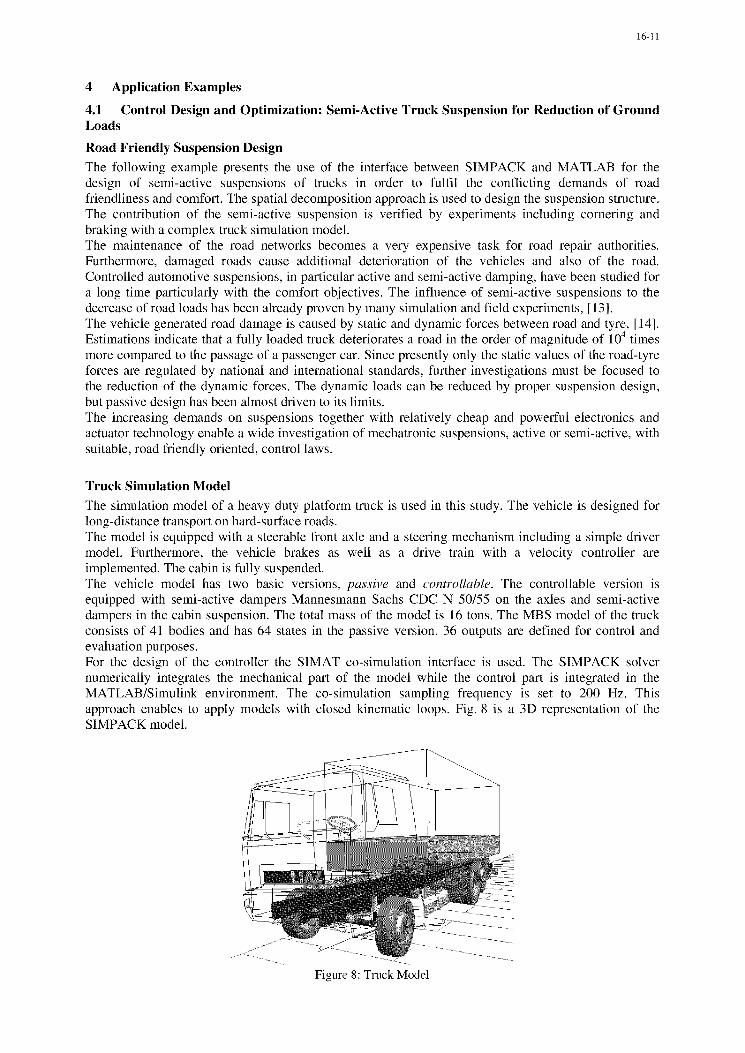
The simulation model of a heavy duty platform truck is used in this study. The vehicle is designed forlong-distance transport on hard-surface roads.The model is equipped with a steerable front axle and a steering mechanism including a simple drivermodel. Furthermore, the vehicle brakes as well as a drive train with a velocity controller areimplemented. The cabin is fully suspended.The vehicle model has two basic versions, passive and controllable. The controllable version isequipped with semi-active dampers Mannesmann Sachs CDC N 50/55 on the axles and semi-activedampers in the cabin suspension. The total mass of the model is 16 tons. The MBS model of the truckconsists of 41 bodies and has 64 states in the passive version. 36 outputs are defined for control andevaluation purposes.For the design of the controller the SIMAT co-simulation interface is used. The SIMPACK solvernumerically integrates the mechanical part of the model while the control part is integrated in theMATLAB/Simulink environment. The co-simulation sampling frequency is set to 200 Hz. Thisapproach enables to apply models with closed kinematic loops. Fig. 8 is a 3D representation of theSIMPACK model.

Figure 8: Truck Model

16-12

Semi-active Suspension Controller DesignThe spatial decomposition approach resolves the contradictory demands on the controller by thestructure of the system, thus this method can be also called more generally spatial distribution ofcontrol tasks. The controlled system is divided into two or more subsystems with different objectivesfor each control. Each system is then optimized using less conflicting criteria or even only one criterionfor one specific task. Certainly, such decomposition is not possible to be applied to all dynamicsystems.The suspension systems of a heavy duty vehicle consist of independent suspensions, such as axlesuspensions, which are mounted between the vehicle axles and the frame, and suspensions of thevehicle cabin, which support the cabin on the frame. The vehicle in Fig. 8 has four independentsuspension systems: (i) front axle suspension, (ii) rear axle suspension, (iii) cabin suspension, and (iv)seat suspension. The strategy is to optimize the axle suspensions exclusively for the objective of roadfriendliness (minimization of road-tire force fluctuation) and the cabin and seat suspension for the ridecomfort.The controller parameters have been designed by simulation with a Multilevel Coordinate Search globaloptimization algorithm. The controller parameters are optimized subsequently. The axle controllers areoptimized in the first sub-process and then the axle controller parameters are fixed and the comfortcontrollers are optimized. The semi-active dampers are controlled by well established control laws. Theaxle suspensions, which are designed as road-friendly oriented, are controlled by the extended groundhook concept. The comfort oriented cabin suspensions are controlled by the skyhook law. The strategyof the controllers and of the optimization is described in detail in [16].The optimization of the axle suspension for minimization of road-tire force fluctuation can result in anincrease of vertical acceleration of the heavy duty vehicle. However, while there are some limits foracceleration transferred to the vehicle cargo, those limits are expected to be fulfilled. A resultingdeterioration of the comfort for the driver is solved by optimizing the cabin suspension and thesuspension of the seat.The spatial decomposition method can be applied to active, semi-active and passive suspensionsystems. Nevertheless, controllable suspension systems can profit from the decomposition significantlymore.

Simulation Results

The simulation scenario consists of an S-shaped track with a curve radius of 120 m. The vehicle isexcited before the curve entrance by a deterministic ramp. The ramp is 0.08 m high and 5.8 m long,ascent and descent lengths are 2.5 m. The vehicle intensively brakes between 3.5 s and 7.5 s from aspeed of 22 m/s down to 4 m/s. The total simulation time is 12 seconds and the initial vehicle velocity isset to 80 km/h.The simulation results for the truck equipped with a passive suspension compared to the semi-activesystem are presented in Fig. 9. The peaks at time 0.5 s are caused by the ramp.Fig. 9a presents the vertical acceleration of the driver. The comfort increase is very significant in thiscase. The passive suspension of the cabin is relatively soft and moreover the vehicle frame, which is thebase for the cabin suspension is better suspended.The road-tyre forces are presented for the outer right tires of the rear axle in Fig. 9b. The influence ofbraking is visible at the time 4 s. A reduction of road-tire forces is observable.

16-13

x 10418 5."5• " [ L

- pasivepassive4semiactive 5 - semi-active

45 semi i . A

4,5 -

'I I *.. - ;-"

S~2.5

22P _..0 .........................

j' 2.5,-

,S.A ... _........_....._...._....._._-_-_- -_-_- -_-_

4 2 6 10 1"0 2 4 6 a 10 12Time [s] Time [s]

Figure 9: Cabin acceleration and road tire forces of truck

The simulation results indicate that the vehicle equipped with a semi-active suspension designed withthe spatial decomposition control profits from a decrease of vertical acceleration and vertical road-tireforces. Generally, the simulation experiments have proved the potential of improvement of roadfriendliness by semi-active damping for vehicle maneuvers.

4.2 Interaction of Aircraft and Landing Gear

Conventional Design ProcessA landing gear of a large transport aircraft has to accomplish a variety of functions. Among others, ithas to:"• dissipate the energy of the vertical velocity at touch-down,"• suspend bumps from uneven runways/taxiways and provide a satisfying rolling comfort.Modern transport aircraft are complex constructions. Their development requires a high level of specialknowledge and experience on a multitude of disciplines. Therefore, many aircraft manufacturersconfide a specialist with design and fabrication of the landing gear. As a rule, a basic design data set isdefined at an early development stage containing, for example, mass and geometry data, configuration,specifications and operating envelopes. Provided with these basic data, the landing gear manufacturerdesigns a landing gear appropriate for the defined aircraft. Parallel to the work on the landing gear, the"airframer" develops and manufactures the airframe according to the ground load cases set up incooperation of both partners. The limited knowledge about the partner's part often leeds to calculationand certification cases where simple models represent the other component, e.g. the "drop-test"-modelwith an equivalent single mass representing the airframe for the design of the landing gear shockabsorber. This parallel strategy has the advantage that the development process can rely on fixed data;iteration loops caused by alterations of the basic design data due to optimization results of the partnerare avoided.On the other hand, the dynamic behavior of the combined system which is, in case of high structuralflexibility, decisively influenced by dynamical interactions cannot be evaluated. A simple example shallillustrate this effect [17]: A large transport aircraft is rolling, at high velocity, over two sinusoidalbumps of a height of 3.8cm (1.5in), 21m (70ft) apart, Fig. 10. If this case is calculated with aconventional rigid airframe model, we receive a result for the applied vertical acceleration in thecockpit of 0.2g, Fig. 10, curve 1. Including the elasticity of the airframe, the maximum acceleration ofthe cockpit triples because of resonance phenomena, Fig. 10, curve 2.

16-14

vertical cockpit acceleration [g]

10.6 v, =60 m/s -2rigid aircraft model 0.4 elastic aircraft model

0.2

0

-0.2

-0.4 SI

-0.6.. . .. . . . .. . .. tim e [s ]

0 0.5 1 1.5 2

Figure 10: Comparison Between Rigid and Elastic Modeling

Integrated design

The later problematic interaction effects between airframe and landing gear are detected, the smaller isthe available design freedom for alternative solutions - with progressively climbing costs. Preventiveefforts should therefore take effect as early as possible to implement necessary adoptions to the designquickly, efficiently and without loss of performance.Consideration of component interactions due to structural elasticities influences the entire designprocess. Neither airframer nor landing gear manufacturer can rely on a fixed set of basic design data;the level of detail of the basic design data set necessary to assess the most important influences on thesystem dynamics enforce the inclusion of data which are subject to permanent changes during thedevelopment process. This requires alterations on the level of design strategy, e.g distribution ofresponsibility or data handling, as well as modifications of the computational methods.Compared to the conventional design strategy where the manufacturers develop their product in awidely independent development process, Fig. 11, left, the so-called "Integrated Design" strategy leadsto a close cooperation [18]. The final solution matures out of the development and optimization processof both manufacturers, Fig. 11, right. Unfavorable lay-outs are detected early and can be corrected withcomparatively small effort.Basis for such a coupled design process is an aircraft/landing gear model comprising data from both theairframer and the landing gear manufacturer.

L/G-manufacturer ,,airframer" L/G-manufacturer ,,airframer"

optimzingoptimizing

I }' optimizing7ove railI

I yz ,' . ~~~--rbehavior

C 9

the Iloop" ... :N

Figure 11: Conventional and Integrated Design Process

Fig. 12 shows an example of such an integrated model for dynamic analysis of airframe / landing gearinteraction. A multibody simulation model is assembled, using the interfaces described in Sec. 3. Thedata comes from a number of different sources - for the airframe, usually a FEA model exists; CAD

16-15

models are used to build the simulation model of the landing gears; measurement data enters thesimulation for the modeling of the runway and the tires; controllers are imported as code from a controldesign tool; finally, force laws describing the dynamic behavior of the shock absorbers are programmedand introduced via the programming interface. Simulation runs cover the whole operational envelope onthe ground, i.e. touch-down, taxiing, cornering, push-back, and take-off. After the evaluation the resultsare passed back to the relevant disciplines, most notably forces for stress calculation and certificationpurposes. Such an integrated design has been performed in the German Flexible Aircraft project [171.

fuselage I wing(from FEA) •"

controller r,(from CAGE) Riw-ii-

(mneasurements)

* landing gear model

Oleo (user defined force element)

tyre model(measurements)

Figure 12: Multidisciplinary simulation model of transport aircraft

5 Summary and Outlook

Numerical simulation is an invaluable tool for the integration of system components. It allows the userto analyze his system up to any chosen degree of complexity, to determine physical variables at anygiven point of the system, to change design parameters and perform numerical optimizations, and, bydoing so, to keep the costs of the vehicle design down.While the simulation tools have become very sophisticated in their own domains, the simulation ofcomplex systems calls for multidisciplinary simulation. This can be achieved by the coupling of theexisting codes. For this purpose, interfaces between the codes have to be developed. These interfaceshave to take into consideration the nature of the description of the physical model, numerical propertiesof the respective simulation methods, and software and hardware implementation issues.Multibody system analysis is a powerful tool for multidisciplinary analysis of mechanical andmechatronic systems. For the efficient employment of an MBS analysis, a multitude of engineeringdisciplines have to be considered in the simulation. Combinations of different CAE (computer aidedengineering) tools, like MBS, CAD, FEA, and CACE, allow the computation and evaluation of acomplex system with the desired accuracy and in affordable computation times. MBS as the analysistool of the overall system behavior can form the center element of this multidisciplinary designenvironment.

6 Bibliography

[1] W. Rulka. Effiziente Simulation der Dynamik mechatronischer Systeme fir industrielleAnwendungen. Dissertation an der TU Wien. DLR IB 532-01-06. Oberpfaffenhofen, Germany,2001.

[2] A. Veitl, T. Gordon, A. van de Sand, M. Howell, M. Valasek, 0. Vaculin, P. Steinbauer.Methodologies for Coupling Simulation Models and Codes in Mechatronic System Analysis andDesign. Veitl, A.; Gordon, T. In: The Dynamics of Vehicles on Roads and Tracks; Supplement toVehicle System Dynamics, Vol. 33, pp 231-243, 2000.

[3] R. Kibler, W. Schiehlen. Vehicle Modular Simulation in System Dynamics. In: InternationalConference on Multi-Body Dynamics - New Techniques and Applications, IMechE ConferenceTransactions 1998-13.

[4] W. Kortim, W. Rulka, M. Spieck: Simulation of Mechatronic Vehicles with SIMPACK. MOSIS97, Ostrava, Czech Republic, 1997.

[5] 0. Wallrapp. Standardization of Flexible Body Modeling in Multibody System Codes. Part i:Definition of Standard Input Data. Mech. Struc. & Mach., 22(3), 1994, pp. 283 - 304.