Defending Continuous Collision Detection against Errors

Huamin Wang∗

The Ohio State University

Abstract

Numerical errors and rounding errors in continuous collision de-tection (CCD) can easily cause collision detection failures if theyare not handled properly. A simple and effective approach is to useerror tolerances, as shown in many existing CCD systems. Unfor-tunately, finding the optimal tolerance values is a difficult problemfor users. Larger tolerance values will introduce false positive ar-tifacts, while smaller tolerance values may cause collisions to beundetected. The biggest issue here is that we do not know whetheror when CCD will fail, even though failures are extremely rare. Inthis paper, we demonstrate a set of simple modifications to make abasic CCD implementation failure-proof. Using error analysis, weprove the safety of this method and we formulate suggested toler-ance values to reduce false positives. The resulting algorithms aresafe, automatic, efficient, and easy to implement.

Keywords: Floating-point arithmetic, rounding error, numericalerror, continuous collision detection, quadratic and cubic solver.

CR Categories: I.3.7 [Computer Graphics]: Three-DimensionalGraphics—Animation.

Links: DL PDF

1 Introduction

Detecting the existence of exact vertex-triangle or edge-edge inter-section within a time step is the fundamental step in continuous col-lision detection (CCD). Due to numerical and rounding errors, thedetection result may be false in two ways: false negatives, whenCCD fails to detect real collision events; and false positives, whenCCD reports collisions while real ones do not happen. Since falsenegatives have more severe consequences than false positives, theyare considered as collision detection failures, which must be strictlyavoided. Proposed by Bridson et al. [2002], a typical approach usedin existing systems is to report more collision events than necessaryby setting error tolerance thresholds. This approach can effectivelyreduce collision failures, but it is still not clear how large the toler-ances must be to avoid failures completely. To play it safe, user typ-ically chooses larger tolerance values, but the extra false positivesmay trigger other problems, such as visual artifacts, computationalburden, and convergence issues in collision handling. To solve thisproblem, Brochu and Bridson [2012] studied CCD from a new geo-metric perspective and they formulated a collision predicate that caneliminate both false negatives and false positives. Unfortunately, it

∗Email: whmin@cse.ohio-state.edu

Figure 1: After a set of simple modifications, cubic-based CCD al-gorithms can become failure-proof when simulating the animationof a bow knot, in which complex collisions occur.

is computationally expensive due to more arithmetic operations in-volved in exact and interval arithmetic, the latter of which is appliedto reduce the use of more expensive exact arithmetic.

A typical CCD method solves a cubic equation to find the timewhen two primitives are coplanar and uses it to detect intersection.Since the use of error tolerances has already demonstrated its effec-tiveness in this method, an important question is: can it be strictlyfailure-proof? Obviously, an algorithm is trivially and uselessly“failure-proof”, if it always reports positive. So our real interest isto avoid failures and reduce false positives at the same time. Un-fortunately, our research showed that it is difficult to limit the falsepositives caused by existing algorithms. To handle this issue, ouridea is to introduce a number of conditions, under which vertex-triangle and edge-edge tests are guaranteed to be failure-proof. Ifany condition is not satisfied, we resort to vertex-edge CCD test,which reports a collision if the vertex-edge distance drops below acertain threshold within a time step. By using a sufficiently largedistance threshold, we ensure the detection of any collision event.

While our idea is simple, its implementation forces us to face twocritical challenges. The first challenge is how to formulate vertex-edge test. Computing the time when the Euclidean vertex-edgedistance is equal to a threshold involves solving a quartic equa-tion, which is computationally expensive and susceptible to moreerrors. The volume-based geometric predictor proposed by Brochuand Bridson [2012] can detect the short distance without computingthe time, but it is not robust against rounding errors if not using ex-act arithmetic. The second challenges is how to evaluate the overalltest error. Since the numerical error caused by the cubic solver andthe rounding errors caused by floating-point arithmetic coexist, wecannot perform direct error analysis as in [Wilkinson 1994].

In this work, we made the following contributions: 1) a novel im-plementation of vertex-edge test with O(ε

14 ) relative error, in which

ε is machine epsilon; 2) systematic error analysis of the cubic-basedtests; 3) a set of simple modifications to make cubic-based testsfailure-proof; and 4) the formulation of lower bounds on the errortolerances. Compared with existing methods, our method is:

Safe. We prove that cubic-based CCD algorithms can be un-conditionally failure-proof after applying our methods.

1 14 226 ; 3R B B 1 12 22 2 2725 ; 2080B B

VT_CCD

EE_CCD

VE_CCD VV_CCD

×3

×4

×2 122 21678D B

2311B

3 14 23 264 ; 64B B

3 14 23 264 ; 64B B

144B

144B

Figure 2: Our CCD tests and their error tolerance values. A VTtest may call the VE test up to three times, and an EE test maycall the VE test up to four times. The choices of tolerance valueswill be discussed in Section 4. Note that they have been slightlyincreased in our analysis, so they can be computed using floating-point arithmetic directly.

Simple. Our modifications are simple and can be easily incor-porated into existing systems.

Efficient. Our experiment shows that the computational over-head of our method is only a fraction of the original test cost.

Automatic. Based on error analysis, CCD algorithms can au-tomatically determine all of the tolerance values. User does notneed to specify a single parameter.

Accurate. Our method computes the tolerance values by min-imizing the vertex-triangle or edge-edge distance when a false pos-itive occurs. So using them can reduce false positives.

2 Related Work

Collision detection. Errors and degeneracies in proximityand intersection tests have been studied [Gilbert et al. 1988; Gold-berg 1991; Shewchuk 1996; Larsen et al. 2000] in the past. Basedon these tests, researchers developed the discrete collision detec-tion approach [Baraff et al. 2003; Volino and Magnenat-Thalmann2006] that tests collisions at discrete time instants only. While thisapproach is robust, it may miss collisions when objects move fast,known as the tunneling artifact. One solution is to gradually ad-vance the simulation time until a collision happens, as proposed byTang et al. [2010]. Alternatively, the continuous collision detectionapproach computes the possible collision time when two primitivesare coplanar. For vertex-triangle and edge-edge collisions, the timecan be found by solving cubic equations as Provot [1997] showed.Bridson et al. [2002] improved the robustness of this method byusing rounding error tolerances on vertex-plane distances, line-linedistances, and barycentric coordinates. However, how to find opti-mal error tolerances is a tricky problem and there is often no way toguarantee the detection of every collision event. To avoid collisionfailures, Brochu and Bridson [2012] proposed to separate collisiondetection from collision time query, and developed a root-parity-based CCD algorithm using exact arithmetic. The robustness ofcollision tests can also be improved by reporting a collision whenthe distance between two primitives is less than a threshold as S-tam [2009] suggested. This requires solving six-order polynomialequations, when handling vertex-triangle or edge-edge collisions.

Collision culling and handling. Recent research in collisionculling has resulted in a number of efficient techniques [Schvartz-man et al. 2010; Pabst et al. 2010; Lauterbach et al. 2010; Tanget al. 2011; Zheng and James 2012]. Our method is fully compat-ible with them. Once collisions are found, the next issue is howto resolve collisions by applying collision responses on primitives.This can be difficult in complex multi-collision cases. A typical so-lution to unresolved collisions after a number of processing steps isto treat them as rigid bodies in impact zones [Provot 1997; Bridsonet al. 2002; Huh et al. 2001; Harmon et al. 2008]. Thomaszews-

Algorithm 1 VV CCD(x0i , x1

i , x0j , x1

j , D2)

Compute x ji and v ji;T← Clamp(−(x ji · v ji)/(v ji · v ji), 0, 1);for every root t ∈ T do . Proximity test

if∥∥∥x ji + tv ji

∥∥∥2

2≤ D2 + δ then return true;

ki et al. [2008] suggested to process collisions asynchronously formore accurate collision responses, although their method still relieson synchronous collision handling to avoid remaining collisions. Apurely asynchronous system was developed by Harmon et al. [2009;2011], which guarantees that each collision process can be done in afinite time and its result is free of penetrations. Ainsley et al. [2012]combined an asynchronous system with continuous collision detec-tion, which reduces the number of rescheduling events and makesthe system faster. Since the use of our method in CCD reduces falsepositives and makes the collision time more accurate, we believe itwill improve the robustness of collision handling as well.

3 Continuous Collision Detection

In this section, we will present our algorithms for vertex-vertex(VV) CCD test, vertex-edge (VE) CCD test, vertex-triangle (VT)CCD test, and edge-edge (EE) CCD test. Our basic idea is to incor-porate the VV test into the VE test, and the VE test into the VT andEE tests, as Figure 2 shows. We note that the pseudo code given inthis section slightly differs from the descriptions, due to the use oferror tolerances. We will discuss them later in Section 4.

3.1 Vertex-Vertex Collision Detection

Vertex-vertex CCD reports a collision, if the Euclidean distance isshorter than a threshold D at any time t between the starting time 0and the ending time 1. The Euclidean distance is defined as: (x ji +tv ji) · (x ji + tv ji), in which x ji = x0

ji = x0j − x0

i and v ji = (x1j −

x1i ) − (x0

j − x0i ). We compute t0 when the distance is minimized as:

t0 = −(x ji ·v ji)/(v ji ·v ji). Since t0 must be in [0, 1], we apply Clampon it. After that, we compute the squared distance at t0. If it is lessthan D2, the algorithm reports a collision as Algorithm 1 shows.

3.2 Vertex-Edge Collision Detection

Vertex-edge CCD reports a collision if the Euclidean distance isless than a threshold R. Let x0 be a vertex and xix j be an edge. TheEuclidean distance between the vertex and the edge line at time t

is: ‖(x0i+tv0i)×(x ji+tv ji)‖2‖x ji+tv ji‖2

. Finding the time when it gets minimized (orequal to R) is difficult without solving a complex equation. Butsince ||x||1 ≤

√3||x||2 ≤ 3||x||∞ for any x, if the Euclidean distance

is less than R at t, then the following condition must be satisfied:

F0i j(t) =∥∥∥(x0i + tv0i) × (x ji + tv ji)

∥∥∥1− S

∥∥∥x ji + tv ji

∥∥∥∞≤ 0 (1)

in which S = 3R. So instead of finding tE0 that minimizes the Eu-

clidean distance, we define the time t0 as the local minimum ofF0i j(t) closest to tE

0 , which may or may not be the global mini-mum. Since F0i j(tE

0 ) ≤ 0 when a collision occurs, we must haveF0i j(t0) ≤ 0. In addition, we need to consider the boundary casewhen the vertex-edge distance is not the vertex-line distance (i.e.,when the vertex’s projection on the edge line is outside of the edge).By formulating the test into a constrained optimization problem, wemust be able to find t0 from five Karush–Kuhn–Tucker cases.

Case 1. t0 = 0 or 1.

Algorithm 2 VE CCD(x00, x1

0, x0i , x1

i , x0j , x1

j , R)

Compute {x0i, xi j} and {v0i, vi j};

T←{0, 1,− x ji±y ji

u ji±v ji,−

x ji±z jiu ji±w ji

,−z ji±y jiw ji±v ji

}; . Case 1 and 3

xa ← v0i × v ji;xb ← x0i × v ji + v0i × x ji;xc ← x0i × x ji;for every component k in xa and xb do

if |k| ≤ ρ then k ← 0;T← T

⋃Quadratic Solver(xa.x, xb.x, xc.x); . Case 4

T← T⋃Quadratic Solver(xa.y, xb.y, xc.y);

T← T⋃Quadratic Solver(xa.z, xb.z, xc.z);

for every at2 + bt + c = 0 in Case 2 doT← T

⋃{−b/2a}; . Case 2

for every root t ∈ T do . Proximity testCompute xt

0i, xtji; . xt

0i ← x0i + tv0i

if 0 ≤ t ≤ 1 and xtji · x

tji ≥ λ

2 and 0 ≤ xt0i · x

tji ≤ xt

ji · xtji and

F0i j(t) ≤ ψ then return true;if VV CCD(x0

0, x10, x0

i , x1i , D2) or

VV CCD(x00, x1

0, x0j , x1

j , D2) then return true;return false;

Case 2. The components in x ji+t0v ji have unique magnitudes andno component in (x0i + t0v0i) × (x ji + t0v ji) is equal to zero. In thiscase, F0i j(t0) can be considered as a quadratic function locally at t0and the solution of F′0i j = 0 gives t0. There are eight possibilitiesin

∥∥∥(x0i + tv0i) × (x ji + tv ji)∥∥∥

1and six possibilities in

∥∥∥x ji + tv ji

∥∥∥∞

.Due to the symmetry, only 24 time candidates are unique.

Case 3. At least two components of x ji + t0v ji have the samemagnitude at time t0. If so, we find t0 by solving a linear equation.Since there are three components and each component can be eitherpositive or negative, there are at most six unique candidates.

Case 4. At least one component of (x0i +t0v0i)×(x ji +t0v ji) is zeroat time t0. If so, we can find t0 by solving the quadratic equation.There are three equations and six collision time candidates at most.

Case 5. The time t0 is the vertex-vertex collision time betweenx0 and xi, or x0 and x j.

Degenerate cases. Although degenerate cases are rare, we stillneed to examine them to ensure the robustness of vertex-edge C-CD. First of all, any linear equation may be trivially reduced to aconstant in Case 3. If so, t0 has no influence on

∥∥∥x ji + tv ji

∥∥∥∞

and wecan find it from other cases. Similarly, if any quadratic equation1 inCase 4 is reduced to a constant, we find t0 from other cases. If allequations in Case 3 and 4 are trivial, the choice of t has no influenceon F0i j(t) and we can simply set t0 = 0 or 1. This may happen whenthe vertex-line distance is relatively static. If the quadratic equationin Case 2 is reduced to a linear equation or even a constant, thenF0i j(t) must be minimized at t0 = 0 or 1, which is covered by Case1. We note that we have not discussed

∥∥∥x ji + t0v ji

∥∥∥∞

= 0, whichmakes Equation 1 ineffective. We will study it in Subsection 4.3.

Summary. Given the five cases, we can formulate our vertex-edge CCD algorithm in two steps as Algorithm 2 shows. In the firststep, it computes a set of collision time candidates. In the secondstep, it verifies whether F0i j(t) is indeed small at each candidate.Although there are many candidates, only a few are valid (between0 and 1) and need further verification. The average number of validcandidates is about seven as our experiment shows.

1Our quadratic solver (in Appendix A) can handle the degenerate casewhen a quadratic equation is reduced to a linear equation.

One question is how to determine the distance threshold D to cap-ture missed collision events by vertex-vertex CCD. Let t0 be thetime when F0i j(t) is minimized and the time tE

0 be the time when theEuclidean distance is minimized. If the vertex’s projection is out-side of the edge at tE

0 , we can set D ≥ R. If the vertex’s projection isinside of the edge at t0, vertex-vertex CCD is unused. So collisionsare missed when the vertex’s projection is outside at t0 but inside attE0 only, as Figure 3a shows. Fortunately, since t0 is the minimum

of F0i j(t) closest to tE0 , F0i j(t) ≤ 0 and the vertex-line distance must

be shorter than S at any t ∈ [t0, tE0 ]. When the vertex’s projection

moves from the interior of the edge to the exterior, there must ex-ist time t when the vertex’s projection is at an endpoint. We useD ≥ S = 3R to capture this collision by vertex-vertex CCD at t.

3.3 Vertex-Triangle Collision Detection

In our vertex-triangle CCD algorithm shown in Algorithm 3, weapply vertex-edge CCD after the cubic-based test [Provot 1997;Bridson et al. 2002], to avoid missed collisions. The closed-formsolution of a cubic equation requires the cubic root, which cannotbe correctly rounded under the IEEE 754 standard. Instead, a nu-merical solver finds t0, such that the residual error at t0 is below athreshold µ. The use of this threshold2 suffers from two problems.

Small triangle. The cubic function F(t) = (x01 + tv01) · (x21 +tv21) × (x31 + tv31) is proportional to the Euclidean vertex-planedistance times the triangle area at time t. So if the triangle is smallat t0, the residual error is also small, even when the vertex-planedistance is still large. As a result, proximity test will fail at time t0.

Parallel motion. Another problem happens when the vertexmoves nearly parallel to the triangle plane, in which case the residu-al error becomes small even before the vertex intersects the triangle.

Due to the motion of the primitives, it is possible to notice suchdegenerate problems only at t0 and in its neighborhood. So we can-not detect them as special cases without computing t0. To preventthem from causing collision failures, we apply vertex-edge CCDafter proximity test. If the triangle is small when a collision hap-pens, the vertex must be close to a triangle edge and this collisioncan be detected by vertex-edge CCD. Meanwhile, if a vertex movesnearly parallel to the triangle plane, it must get sufficiently close toa triangle edge before it intersects the triangle. So vertex-edge CCDcan detect this collision as well.

3.3.1 Errors and False Positives

Here we would like to study the overall error without consideringthe rounding errors. Our goal is: 1) to eliminate false negatives;and 2) to reduce false positives as much as possible.

Let µ be the convergence threshold of the cubic solver, σ be thethickness threshold in the vertex-triangle proximity test, and R bethe Euclidean distance threshold in vertex-edge CCD. Let t0 be theexact vertex-triangle intersection time (such that F(t0) = 0) andt0 be its computed version (such that |F(t0)| ≤ µ). By definition,F(t) = A(t)C(t), in which A(t) is twice the triangle area and C(t)is the vertex-plane distance. Since |F(t0)| ≤ µ, instead of testingwhether |C(t0)| ≤ σ, we test whether |A(t0)| ≥ τ = µ/σ. If so, wehave |C(t0)| ≤ σ and the test proceeds. If not, we do vertex-edgeCCD. Assuming that |F(t)| ≤ µ for any t in [t0, t0] (in AppendixB), we claim every exact collision event will be detected by settingR = µ

13 . To prove this, we show that if an exact collision fails the

vertex-triangle proximity test, it must pass vertex-edge CCD.2A numerical solver may use other convergence criteria, but they are

ineffective once the rounding error becomes dominant.

x0t0 S

t

δ

x0

tE0t

xi xjt00t

δtx0

δ

x0t

δx0

t0

δ δt0

δ

(a) Vertex-edge case

x0t0 S

t

σ

x0

tE0t

xi xjt00t

σtx0

σ

x0t

σx0

t0

σ σt0

σ

(b) A(t0) ≤ τ

x0t0 S

t

σ

x0

tE0t

xi xjt00t

σtx0

σ

x0t

σx0

t0

σ σt0

σ

(c) A(t0) ≥ τ

x0t0 S

t

σ

x0

tE0t

xi xjt00t

σtx0

σ

x0t

σx0

t0

σ σt0

σ

(d) A(t) = τ

x0t0 S

t

σ

x0

tE0t

xi xjt00t

σtx0

σ

x0t

σx0

t0

σ σt0

σ

(e) Projected onto an edge

Figure 3: Vertex-edge and vertex-triangle CCD cases. When the vertex x0 moves along its trajectory (in a dashed line) over time, the edgelength and the triangle size may vary. The red lines and triangles represent the upper bounds on the vertex-line and vertex-plane distances.

Algorithm 3 VT CCD(x00, x1

0, x01, x1

1, x02, x1

2, x03, x1

3)

Compute {x01, x21, x31} and {v01, v21, v31};a← v01 · v21 × v31;b← x01 · v21 × v31 + v01 · v21 × x31 + v01 · x21 × v31;c← x01 · v21 × x31 + x01 · x21 × v31 + v01 · x21 × x31;d ← x01 · x21 × x31;T← {0, 1}

⋃Cubic Solver(a, b, c, d, µ);

for every root t ∈ T do . Proximity testCompute xt

01, xt21, xt

31; . xt01 ← x01 + tv01

N = xt21 × xt

31;if ‖N‖∞ ≥ τ and

max(∥∥∥xt

21

∥∥∥∞,∥∥∥xt

31

∥∥∥∞,∥∥∥xt

31 − xt21

∥∥∥∞

)η ≤ ‖N‖∞ and

0 ≤ N · xt21 × xt

01 ≤ N · N and0 ≤ N · xt

01 × xt31 ≤ N · N and

0 ≤ N · xt21 × xt

01 + N · xt01 × xt

31 ≤ N ·N then return true;if VE CCD(x0

0, x10, x0

1, x11, x0

2, x12, R) or . /* Additional tests */

VE CCD(x00, x1

0, x02, x1

2, x03, x1

3, R) orVE CCD(x0

0, x10, x0

3, x13, x0

1, x11, R) then return true;

return false;

Triangle area test. The proximity test fails because A(t0) ≤ τ attime t0, as Figure 3b shows. If we also have A(t0) ≤ τ, then themaximum squared radius of the triangle inner circle is

√3

18 τ and at

least one squared Euclidian vertex-edge distance is less than√

318 τ at

time t0. So by setting R2 ≥√

318 τ, we can get this collision reported

by vertex-edge CCD. On the other hand, we may have A(t0) ≥ τ(Figure 3c). Since A(t) and the vertex’s projection are two con-tinuous functions of time, there must exist time t in [t0, t0], suchthat A(t) = τ and the vertex’s projection is within the triangle (Fig-ure 3d), or A(t) ≥ τ and the vertex’s projection is on a triangle edge(Figure 3e), the latter of which may not happen if the vertex’s pro-jection is always within the triangle from t0 to t0. If the first eventhappens, we have C(t) ≤ µ/τ = σ and we can set R2 ≥ σ2 +

√3

18 τ todetect this case at time t. If the second event happens, the vertex-edge distance is less than σ at time t and we need R ≥ σ. We willrefer to the idea of defining two events and finding the time whenan event happens as the two-event analysis in the rest of this paper.

One interesting observation from the above analysis is that if A(t) ≤τ at any t ∈ [t0, t0], we can replace t0 by t and use the above anal-ysis to conclude that R2 ≥ σ2 +

√3

18 τ is also sufficient to get suchcollisions detected. So we need to consider only the cases whenA(t) ≥ τ for any t ∈ [t0, t0] next.

Barycentric test. If A(t0) > τ, the proximity test can fail onlybecause of the barycentric test, in which case the vertex’s projec-tion is outside of the triangle at time t0. Let t be the time when thevertex’s projection intersects a triangle edge. Since A(t) ≥ τ accord-ing to the previous analysis, the vertex-plane distance is bounded byσ and we can use R ≥ σ to detect such collisions at time t.

Algorithm 4 EE CCD(x00, x1

0, x01, x1

1, x02, x1

2, x03, x1

3)

Compute {x20, x10, x32}, {v20, v10, v32};a← v20 · v10 × v32b← x20 · v10 × v32 + v20 · v10 × x32 + v20 · x10 × v32;c← x20 · v10 × x32 + x20 · x10 × v32 + v20 · x10 × x32;d ← x20 · x10 × x32;T← {0, 1}

⋃Cubic Solver(a, b, c, d, µ);

for every root t ∈ T do . Proximity testCompute xt

20, xt10, xt

32; . xt20 ← x20 + tv20

N = xt10 × xt

32;if ‖N‖∞ ≥ τ and max(

∥∥∥xt10

∥∥∥∞,∥∥∥xt

32

∥∥∥∞

) · η ≤ ‖N‖∞ and0 ≤ N · xt

20 × xt10 ≤ N · N and

0 ≤ N · xt20 × xt

32 ≤ N · N then return true;if VE CCD(x0

2, x12, x0

0, x10, x0

1, x11, R) or . Additional tests

VE CCD(x03, x1

3, x00, x1

0, x01, x1

1, R) orVE CCD(x0

0, x10, x0

2, x12, x0

3, x13, R) or

VE CCD(x01, x1

1, x02, x1

2, x03, x1

3, R) then return true;return false;

Summary. In conclusion, R2 ≥ σ2 +√

318 τ is sufficient to detec-

t missed collision events by vertex-edge CCD. A simple way toreduce the false positives is make R as small as possible. Givenτ = µ/σ, we can minimize R by setting τ3 =

36µ2√

3, in which case

R3 = 14µ. For simplicity, we use τ = 4µ

23 and R = µ

13 . We will

discuss the changes caused by the rounding errors in Section 4.4.

3.4 Edge-Edge Collision Detection

To detect the collision between two edges x0x1 and x2x3, we for-mulate edge-edge CCD similar to vertex-triangle CCD, except thatthe normal N is defined as the cross product of the two edges. Inthis case, ‖N‖2 is equal to twice the area of the quadrilateral formedby the four vertex projections along the N direction, and the cubicfunction is defined as: F(t) = (x20 + tv20) · (x10 + tv10)× (x32 + tv32).The algorithm suffers from similar problems: small quadrilateral,when the quadrilateral formed by the two edges is small; and per-pendicular motion, when the relative motion of the edges is nearlyperpendicular to N. Our solution again is to use vertex-edge CCD.

3.4.1 Errors and False Positives

By ignoring the rounding errors, we would like to: 1) to eliminatefalse negatives; and 2) to reduce false positives. Let µ be the con-vergence threshold of the cubic solver, σ be the thickness thresholdon the line-line distance, and R be the distance threshold in vertex-edge CCD. By definition, F(t) = A(t)C(t), in which A(t) is twicethe quadrilateral area and C(t) is the line-line distance. Similar tovertex-triangle CCD, the proximity test contains two steps: the areatest: |A(t0)| ≥ τ = µ/σ; and the barycentric test. If a real collisionfails any step, we must use vertex-edge CCD to detect it.

Quadrilateral area test. The proximity test fails because A(t0) ≤τ at time t0. Given a quadrilateral defined by two crossing edges, theshortest distance from any vertex to the other edge must be boundedby half of the shorter edge length. If A(t0) ≤ τ, the shorter crossingedge length cannot exceed

√τ, and the shortest Euclidean vertex-

edge distance is less than√τ

2 at time t0. This means we can usevertex-edge CCD to detect such events by setting R2 ≥ τ

4 . On theother hand, we may have A(t0) ≥ τ. Using the two-event analysispresented in Subsection 3.3.1, we formulate a sufficient condition toget the collision detected: R2 ≥ σ2 + τ

4 . Based on the same analysisin Subsection 3.3.1, we know R2 ≥ σ2 + τ

4 is also sufficient to detectany collision, if A(t) ≤ τ happens at any t ∈ [t0, t0].

Barycentric test. When the barycentric test fails, the edges donot intersect at time t0 in the projected plane. Let t be the timewhen a projected edge intersects the other projected edge’s vertex.As shown previously, we have A(t) ≥ τ and the line-line distance isbounded by σ at t. So R ≥ σ is sufficient.

Summary. In conclusion, R2 ≥ σ2 + τ4 is sufficient to prevent

collision events from being missed. To reduce the false positives,we need to make R as small as possible. Given τ = µ/σ, we canminimize R by setting τ3 = 8µ2, in which case R2 = 3

4µ23 . For

simplicity, we use τ = 2µ23 and R = µ

13 .

4 Error Analysis

Compared with the numerical errors, the rounding errors causedby floating-point arithmetic are more complex. We will study theirproperties in Subsection 4.1 and then discuss their effect in CCD.

4.1 Rounding Error Properties

Let a be a real number, the rounding process converts a into afloating-point number a, such that |a − a| < |a|ε, in which ε ismachine epsilon. The single precision floating-point format us-es ε = 2−23, and the double precision format uses ε = 2−52.The arithmetic operations performed on floating-point numbers arefloating-point arithmetic. According to the IEEE 754 standard, ba-sic floating-point arithmetic operations, including add, subtract,multiply, divide, and square root, must be correctly rounded.In other words, given an exact arithmetic operator ∗ and its floating-point counterpart ~, a~b = ROUND(a∗b) and |a~b−a∗b| ≤ |a∗b|ε.

When there are multiple floating-point operations, rounding errorsare accumulated and the error bounds are not straightforward tocompute. To handle this issue, we propose an error estimation strat-egy based on forward error analysis. Let f be a function containingmultiple arithmetic operations. Its rounding error | f − f | is boundedby: E f = B f ((1 + ε)k f − 1), in which B f is an upper bound on | f |and k f is an exponential coefficient. Assuming that all variables inf are bounded by B0, we can formulate the operations of f into atree and find B f and k f as:• If node i is a leaf, Bi = B0 and ki = 0.• If i is a non-leaf node corresponding to add or subtract

and it has two children l and r, then Bi = Bl + Br andki = max(kl, kr) + 1.

• If i is a non-leaf node corresponding to multiply and it hastwo children l and r, then Bi = BlBr and ki = kl + kr + 1.

We prove the correctness of these rules by the following theorem.

Theorem 4.1. If f is a function made of add, subtract, andmultiply operations, then | f | ≤ B f and | f − f | ≤ E f = B f ((1 +ε)k f − 1), in which B f and k f are calculated using the above rules.Proof. This can be proven by induction. By definition, a leaf nodeis an input variable, so its bound is B0 and its error bound is 0.

Now suppose that Bl, kl, Br, and kr can provide valid bounds forthe children of a non-leaf node. If the node i corresponds to addor subtract, then |i| = |l ± r| ≤ |l| + |r| ≤ Bl + Br, and |i − i| ≤∣∣∣l − l

∣∣∣ + |r − r| +∣∣∣i − (l ± r)

∣∣∣ ≤ Bi((1 + ε)ki−1 − 1) + Bi(1 + ε)ki−1ε =

Bi((1 + ε)ki − 1). If i corresponds to multiply, then |i| = |lr| ≤ BlBr

and |i− i| ≤∣∣∣lr − lr

∣∣∣+ ∣∣∣i − lr∣∣∣ ≤ Bi((1 + ε)kl+kr − 1) + Bi(1 + ε)

kl+krε =

Bi((1 + ε)ki − 1). So Bi and ki are valid for node i as well. �

The Upper Bound B. Our algorithms start with vector compu-tation to obtain relative positions and velocities. To apply Theo-rem 4.1 in error analysis, we would like to derive an upper boundon their vector components. Here we consider the cases when exactcollisions happen only. Let Emax be an upper bound on the edge vec-tors at time 0: E0

max = max{i, j}

∥∥∥∥x0i − x0

j

∥∥∥∥∞

for any edge {i, j}. Let Vmax

be an upper bound on the velocities: Vmax = maxi

∥∥∥x1i − x0

i

∥∥∥∞

. If the

vertex x0 collides with the triangle at a point xtm when t ∈ [0, 1], then

their distance at time 0 must be bounded by 2Vmax. Since the dis-tance from x0

m to any triangle vertex is bounded by E0max, we know

x001, x0

02, and x003 is bounded by E0

max + 2Vmax. By definition, all ofthe relative velocities are bounded by 2Vmax. So B = E0

max + 2Vmaxis an upper bound on the vector components of both the displace-ments and velocities in vertex-triangle CCD. The same analysis canbe applied to edge-edge CCD, except that collision can happen any-where within the two edges. Because of that, there must exist ver-tex i from one edge and vertex j from the other edge, such thatB = E0

max +2Vmax is an upper bound on the displacement from i to j.In practice, this vertex pair can be detected as the one with the min-imum component, and we assume x20 is such a pair in Algorithm 4.We note that B is also an upper bound on the relative positions atany time in [0, 1]. We will use this fact to study the errors of prox-imity tests later. A small issue is B cannot be exactly computed.According to Theorem 4.1, the error involved in B is B((1 + ε)2 − 1)at most, due to two subtract and one add. So to make B valid inboth exact and computed cases, we set: B = (E0

max + 2Vmax)(1 + ε)2.When the primitives move fast, we make B tighter by using relativevelocities. Specifically, we compute the bounding boxes at the s-tarting and ending times, and use their difference to obtain an upperbound V rel

max on the relative velocities, similar to [Selle et al. 2009].We then set Vmax to V rel

max, if V relmax is smaller.

For simplicity, we ignore the errors of the relative positions andvelocities in this section. We will visit them later in Section 5.

4.2 Errors in Vertex-Vertex CCD

We first study the collision time t0 in vertex-vertex CCD. Let∥∥∥x ji

∥∥∥∞≤ B,

∥∥∥v ji

∥∥∥∞

= b ≤ B, m = −x ji ·v ji and n = v ji ·v ji. We knowfrom Theorem 4.1 and Figure 4a that |m − m| ≤ 3Bb((1 + ε)3 − 1)and |n − n| ≤ 3b2((1 + ε)3 − 1). Given n ≥ b2, we have:∣∣∣ m

n −mn

∣∣∣ ≤ ∣∣∣ m−mn

∣∣∣ + t0

∣∣∣ n−nn

∣∣∣ ≤ 10ε(

Bb + 1

). Since t0 ∈ [0, 1], |t0 − t0| ≤∣∣∣t0 −

mn

∣∣∣+∣∣∣ mn −

mn

∣∣∣ ≤ (1 + 10ε

(Bb + 1

))ε+10ε

(Bb + 1

)≤ 12ε

(Bb + 1

).

This conclusion is still valid after applying Clamp on t, whichmakes |t0 − t0| even smaller. Let Fi j(t) =

∥∥∥xi j + tvi j

∥∥∥2

be the Eu-clidean distance at time t. Since

∥∥∥v ji

∥∥∥∞

= b ≤ B, we must have∥∥∥v ji

∥∥∥2≤√

3b and∣∣∣Fi j(t) − Fi j(t)

∣∣∣ ≤ √3b12ε(

Bb + 1

)≤ 24

√3Bε.

Meanwhile,∣∣∣Fi j(t)

∣∣∣ ≤ ∥∥∥xi j

∥∥∥2

+∥∥∥vi j

∥∥∥2≤ 2√

3B, so∣∣∣F2

i j(t) − F2i j(t)

∣∣∣ ≤(4√

3B + 24√

3Bε) · 24√

3Bε ≤ 289B2ε.

The proximity test cannot evaluate F2i j(t) exactly. Since the com-

ponents of x ji, v ji, and x ji + tv ji are all bounded by B, the errorassociated with the components of x ji + tv ji must be bounded by(B+ Bε)ε + Bε ≤ B((1 + ε)2−1). Using Theorem 4.1, we can boundthe proximity test error by:

∣∣∣F2i j(t) − F2

i j(t)∣∣∣ ≤ 3B2((1 + ε)7 − 1) ≤

22B2ε. Together, we have:∣∣∣F2

i j(t) − F2i j(t)

∣∣∣ ≤ 311B2ε and we canset the error tolerance δ = 311B2ε to avoid false negatives.

False positives. When a false positive occurs, We must have:∣∣∣F2i j(t) − D2

∣∣∣ ≤ 2δ. Assuming that D2 is substantially larger than 2δ,

we get the distance error:∣∣∣Fi j(t) − D

∣∣∣ ≤ √2δ ≤ 25Bε12 .

4.3 Errors in Vertex-Edge CCD

We first study the error of F0i j(t), which is related to the vertex-linedistance. To simplify the analysis, we modify F0i j(t) by removingany component in xa or xb, if it is less than ρ = 3B2ε

12 . Let the

result be G0i j(t). Since |F0i j(t) − G0i j(t)| is small, the minimizationof G0i j(t) approximates the minimization of F0i j(t) well.

Case 1 to 4. According to Algorithm 2, there are four cases re-lated to G0i j(t). Let tF

0 be the local minimum of F0i j(t) closest totE0 , t0 be the local minimum of G0i j(t) closest to tF

0 , and t0 be thecomputed version of t0. In the first three cases, t0 is given by simplelinear equations and it is not difficult to see that |G0i j(t0) −G0i j(t0)|and F0i j(t0) − F0i j(tF

0 ) are bounded by B2O(ε). The problem comesfrom Case 4, which requires to solve quadratic equations. LetQ(t) = at2 + bt + c = 0 be the exact quadratic equation, andQ(t) = at2 + bt+ c be the actual equation sent to the solver. The timet0 is computed from Q(t), not Q(t). Since |a − a|, |b − b|, and |c − c|are small, the residual error |Q(t0) − Q(t0)| is also small. Unfortu-nately, |t0 − t0| can be large and it can cause |G0i j(t0) − G0i j(t0)| tobe as large as 688B2ε

12 . In our detailed analysis in Appendix C, we

further show F0i j(t) − F0i j(tF0 ) ≤ 725B2ε

12 for any t ∈ [tF

0 , t0]. So weset the tolerance threshold ψ = 725B2ε

12 in Algorithm 2, to avoid

failures due to the rounding errors.

Case 5. Case 5 is done by vertex-vertex CCD and our job is tofind a suitable distance threshold D in vertex-vertex CCD. Let tE

0 bethe exact time when the Euclidean vertex-edge distance gets mini-mized. We need to study only the cases when the vertex’s projectionis inside of the edge at tE

0 , as discussed in Subsection 3.2. To furtherreduce false positives, we introduce an edge length test. Our goalis to make sure if a real collision fails both the length test and thebarycentric test, it must be detected by vertex-vertex CCD.

• Edge length test. This test prevents F0i j(t) from inviting largefalse positives when the edge is short: l2 ≤ λ2, in which l isthe computed Euclidean edge length at time t0. Since |l2−l2| isat most 3B2((1 + ε)7 −1) ≤ 22B2ε as shown in Subsection 4.2,we know l2 ≤ λ2 + 22B2ε at time t0. If the squared edgelength at time tE

0 is also less than λ2 + 22B2ε, given the vertex-line distance short than R, we can detect this case by settingD2 ≥ R2 + λ2+22B2ε

4 . If not, the squared edge length at time tE0 is

greater than λ2 +22B2ε. Since tF0 is a local minimum of F0i j(t)

closest to tE0 and F0i j(tE

0 ) ≤ 0, we know F0i j(t) ≤ 725B2ε12 , for

any t ∈ [tE0 , t0]. By the definition of F0i j(t), the vertex-line dis-

tance is bounded by 725B2ε12

√λ2+22B2ε

+S , if l2 ≥ λ2 +22B2ε at time t.By defining two events: 1) l2 = λ2 + 22B2ε and 2) the vertex’sprojection is an endpoint of the edge, we apply the two-eventanalysis in Subsection 3.3.1 to derive a sufficient condition:

D2 ≥ λ2+22B2ε4 +

(725B2ε

12

√λ2+22B2ε

+ S)2

, using which vertex-vertexCCD detects the relevant collision at certain time t ∈ [tE

0 , t0].

• Barycentric test. After the edge length test, the barycentrictest may still fail. Passing the edge length test means l2 ≥ λ2

at time t0, or l2 ≥ λ2 − 22B2ε. Since barycentric weights arealso calculated using dot products, their errors are boundedby 22B2ε and the barycentric test error is bounded by 44B2ε.

2B3, 3

4B3, 4

2B2,2 B, 0 2B2,2

12B3, 6

18B3, 7

B, 0

2B3, 3

2B2,2

2B3, 3

6B3, 5

B, 0 6B3,5 6B3,5 6B3,5

B2, 5

2B2, 6

B, 2 B, 2 B, 2 B, 2

B2, 5 4B2, 13

8B2, 14

2B2,6

12B2, 15

2B2,6 2B2,6 2B2,6 2B2,6 2B2,6

4B2, 13 4B2, 13

B, 0

B2, 1

B, 0

B2, 1 B2, 1 B2, 1

2B2, 2

3B2, 3

(a) Dot product

2B3, 3

4B3, 4

2B2,2 B, 0 2B2,2

12B3, 6

18B3, 7

B, 0

2B3, 3

2B2,2

2B3, 3

6B3, 5

B, 0 6B3,5 6B3,5 6B3,5

B2, 5

2B2, 6

B, 2 B, 2 B, 2 B, 2

B2, 5 4B2, 13

8B2, 14

2B2,6

12B2, 15

2B2,6 2B2,6 2B2,6 2B2,6 2B2,6

4B2, 13 4B2, 13

B, 0

B2, 1

B, 0

B2, 1 B2, 1 B2, 1

2B2, 2

3B2, 3

(b) Computing a and d

2B3, 3

4B3, 4

2B2,2 B, 0 2B2,2

12B3, 6

18B3, 7

B, 0

2B3, 3

2B2,2

2B3, 3

6B3, 5

B, 0 6B3,5 6B3,5 6B3,5

B2, 5

2B2, 6

B, 2 B, 2 B, 2 B, 2

B2, 5 4B2, 13

8B2, 14

2B2,6

12B2, 15

2B2,6 2B2,6 2B2,6 2B2,6 2B2,6

4B2, 13 4B2, 13

B, 0

B2, 1

B, 0

B2, 1 B2, 1 B2, 1

2B2, 2

3B2, 3

(c) b and c

6B2, 5

2B2, 3

4B2, 4

12B2, 6

18B2, 7

2B2, 3 2B2, 3

2B2,2 B, 0 2B2,2 B, 0 2B2,2 B, 0 6B2,5 6B2,5 6B2,5

12B2 15

B2, 5

2B2, 6

B2, 5 4B2, 13

8B2, 14

12B , 15

4B2, 13 4B2, 13,

B,2 B,2 B,2 B,2 2B2,6 2B2,6 2B2,6 2B2,6 2B2,6 2B2,6

(d) Computing N

6B2, 5

2B2, 3

4B2, 4

12B2, 6

18B2, 7

2B2, 3 2B2, 3

2B2,2 B, 0 2B2,2 B, 0 2B2,2 B, 0 6B2,5 6B2,5 6B2,5

12B2 15

B2, 5

2B2, 6

B2, 5 4B2, 13

8B2, 14

12B , 15

4B2, 13 4B2, 13,

B2,2 B2,2 B2,2 B2,2 2B2,6 2B2,6 2B2,6 2B2,6 2B2,6 2B2,6

(e) Computing barycentric weights

Figure 4: Error bounds in collision detection. The red arrows rep-resent multiply and the green arrows represent add or subtract.

The value examined by the barycentric test is equal to the edgelength times the distance of the vertex’s projection to an end-point. So when the barycentric test fails erroneously, the dis-tance of the vertex’s projection to a certain endpoint cannotexceed (44B2ε)2

√λ2−22B2ε

at time t0. Together with the upper bound onthe vertex-line distance at time t0, we get a sufficient condi-

tion: D2 ≥(44B2ε)2

λ2−22B2ε+

(725B2ε

12

√λ2−22B2ε

+ S)2

.

False positives. A false positive can be detected either byvertex-edge CCD itself, or vertex-vertex CCD. Since the error invertex-vertex CCD is small, we can consider D as an upper boundon the squared vertex-edge distance in both cases. To reduce falsepositives, we would like to find the optimal λ that minimizes D.After temporarily ignoring S and performing simplifications, wechoose λ2 = 2080B2ε

12 and we set D2 ≥ (16Bε

14 + S )2 + 522B2ε

12

as a sufficient condition for vertex-edge CCD.

4.4 Errors in Vertex-Triangle CCD

The vertex-triangle CCD algorithm contains four steps: 1) findingthe roots of a cubic equation; 2) testing the triangle area; 3) verify-ing the triangle heights; and 4) testing the barycentric coordinates.

Root finding. The first step is to solve F(t) = at3 + bt2 + ct +d = 0. The difference between each exact root t0 and its computedversion t0 can be caused by two reasons. The first reason is theerrors associated with the coefficients. According to Theorem 4.1,|a−a| and |d−d| are bounded by 6B3((1+ε)5−1) and |b−b| and |c−c|are bounded by 18B3((1 + ε)7 − 1) as Figure 4b and 4c show. Thesecond reason is the errors caused by the cubic solver. Appendix Bshows that our cubic solver guarantees the existence of t0 for everyt0 and |F(t)| ≤ µ for any t ∈ [t0, t0], if µ ≥ 33492B3ε.

Triangle area test. In this step, we test whether the triangle areais sufficiently large at a computed collision time candidate t0. Tosimplify the error analysis, we test

∥∥∥N∥∥∥∞≥ τ, in which τ is an area

threshold. Using Theorem 4.1 and Figure 4d, we know the errorassociated with N is bounded by 2B2((1 + ε)6 − 1) ≤ 13B2ε. Ifthe triangle area test fails, then A(t0) ≤

√3 ‖N‖∞ ≤

√3(τ + 13B2ε)

at time t0. From the analysis in Subsection 3.3, we know R2 ≥τ+13B2ε

6 + r2 is sufficient to get such collisions detected, in whichr =

µ

τ−13B2ε. On the other hand, if a vertex and a triangle passes

the area test, then ‖N‖2 ≥ ‖N‖∞ ≥ τ − 13B2ε. By definition, thevertex-plane distance must be bounded by r. We note that if anycollision satisfies A(t) ≤ τ − 13B2ε for any t ∈ [t0, t0], then R2 ≥τ+13B2ε

6 + r2 is also sufficient to get it detected, according to the

analysis in Subsection 3.3.1. So we assume A(t) ≥ τ − 13B2ε andthe vertex-plane distance is bounded by r for any t ∈ [t0, t0] next.

Triangle height test. When triangles are slim, the rounding er-rors in the barycentric test may cause large false positives. Sowe propose a triangle height test to detect them and send them tovertex-edge CCD instead. Specifically, we compare every trian-gle height with a height threshold η at time t0: η

∥∥∥xi j

∥∥∥∞≤ ‖N‖∞,

in which i j is a triangle edge. Since this test happens after thearea test, we must have ‖N‖2 ≥ τ − 13B2ε. Let h be a triangleheight. If it passes the height test, then h =

‖N‖2‖xi j‖2

≥ τ−13B2ε

‖xi j‖2and

η∥∥∥xi j

∥∥∥∞< ‖N‖∞ + 21B2ε, in which 21B2ε is the error associated

with this test according to Theorem 4.1 (assuming that η ≤ B). Soh ≥ η

√3− 21B2ε

‖xi j‖2≥

η√

3− 21hB2ε

τ−13B2ε. Since τ is going to be substantial-

ly greater than B2O(ε), it is safe to simplify the previous equationinto: 2h ≥ η. Therefore, all of the heights must be greater than η

2 ,if a triangle passes the triangle height test. On the other hand, ifa triangle fails the height test, we must ensure that a real collisionstill gets detected by vertex-edge CCD.

• The height test fails when any triangle edge is shorter than Eat time t0. If any edge is shorter than E at time t0, we cansimply use the condition: R2 ≥ E2

4 . If not, by defining twoevents: 1) the shortest edge length is E and 2) the vertex’sprojection is on a triangle edge, and we can use the two-eventanalysis in Subsection 3.3.1 to derive a sufficient condition:R2 ≥ E2

4 + r2, in which r =µ

τ−13B2εis an upper bound on the

vertex-plane distance at any time t ∈ [t0, t0].

• Otherwise, the height test fails when no edge is shorter thanE at time t0. Using Theorem 4.1, we know η

∥∥∥xi j

∥∥∥∞> ‖N‖∞ −

21B2ε. Since∥∥∥xi j

∥∥∥2≥

∥∥∥xi j

∥∥∥∞

and ‖N‖∞ ≥ 1√

3‖N‖2, at least

one triangle height is less than√

3(η + 21B2εE ). Based on the

previous analysis, we use R2 ≥ 34 (η + 21B2ε

E )2 + r2.

By temporarily ignoring η, we choose E = 214 Bε

12 , in which case

the condition is reformulated into: R2 ≥3(η+4Bε

12 )2

4 + r2.

Barycentric test. The barycentric test computes the barycentricweights and compares them to 0 or N · N. Each weight containsat most 12B4((1 + ε)15 − 1) ≤ 181B4ε error, as Figure 4e shows.So the overall error of each barycentric criterion must be boundedby 24B4((1 + ε)16 − 1) + 12B4((1 + ε)15 − 1) ≤ 565B4ε. If thebarycentric test fails correctly, then the vertex’s projection is outsideof the triangle at time t0 indeed. According to our previous analysisin Subsection 3.3.1, R ≥ r is sufficient to get such cases detected byvertex-edge CCD. If the barycentric test fails erroneously, then thevertex’s projection should still be inside of the triangle at time t0.By definition, the barycentric weight assigned to x1 is equal to ‖N‖2times the edge length ‖x23‖2 times the vertex-edge-line distance l,as Figure 5a shows. Since the vertex and the triangle passed thearea test and the height test, we know ‖N‖2 ≥ τ − 13B2ε and allof the heights are greater than η

2 . Given the fact that no edge canbe shorter than the shortest height, we have l ≤ 1130B4ε

η(τ−13B2ε) . Whena vertex’s projection is within the triangle, its distance to the edgelines is also its distance to the edges. So R2 ≥

(1130B4ε)2

η2(τ−13B2ε)2 + r2 issufficient to get the case detected by vertex-edge CCD at t0.

4.4.1 False Positives

To study false positives, we would like to formulate an upper boundon the vertex-triangle distance at t0 when a false positive happens.

Proximity test. A false positive can occur when it erroneous-ly passes all of the three tests. Based on the previous analysis, we

x1 x1e13e12 φ θ

x2 x3l

x2 x3

13φθ

θ

φβ α

(a) A region formed by six dashlines parallel to the edges, in whicha false positive can exist.

x1 x1e13e12 φ θ

x2 x3h

x2 x3

13φθ

θ

φβ α

(b) A corner point. The distancebetween the corner point and x3 isinversely proportional to the height.

Figure 5: False positives in vertex-triangle CCD.

know the vertex-plane distance is bounded by r at time t0. The ques-tion is what is the distance between the vertex’s projection and thetriangle edges, when a false positive occurs due to the barycentrictest. As we showed previously, the rounding error of a barycentriccriterion is bounded by 565B4ε and the barycentric weight is equalto ‖N‖2 times the edge length times the vertex-edge-line distance.Let e be an Euclidean edge length at time t0. If the vertex’s pro-jection is erroneously treated as if it was inside, then its distance tothe corresponding edge line must be bounded by 565B4ε

e‖N‖2at time t0.

The six criteria used in the barycentric test form six lines aroundthe triangle and a false positive can occur only if the vertex’s pro-jection is within the region surrounded by the six lines, as Figure 5ashows. So instead finding an upper bound on the distance from thevertex’s projection to the triangle, we find an upper bound on thedistance from the six corner points (where the lines intersect) to thetriangle edges. Without loss of generality, let us consider a cor-ner point formed by the barycentric criteria of two edges, as shownin Figure 5b. Let the two edge lengths be e13 and e12. Since thedistance from x3 to the two lines are 565B4ε

e13‖N‖2and 565B4ε

e12‖N‖2, we have

e13 cos θ = e12 cos φ, in which θ and φ are two angles formed by thecorner point and the perpendicular directions. Let α and β be twotriangle angles and we know α+ β+ θ + ϕ = π. This means the linesplitting the angle at x1 into θ and φ must be perpendicular to x2x3.Therefore, e13 cos θ = e12 cosϕ = h, where h is the triangle heightand we know the corner-point-vertex distance must be bounded by565B4εh‖N‖2

. Since a false positive passes both the area test and the heighttest, we have ‖N‖2 ≥ τ−13B2ε and h ≥ η

2 . So the corner-vertex dis-tance must be bounded by 1130B4ε

η(τ−13B2ε) , which is also an upper boundon the distance between the vertex’s projection and the edges. Thisconclusion is valid even if α or β is greater than π

2 , in which caseθ or ϕ is negative. Together the squared vertex-triangle distance isbounded by (1130B4ε)2

η2(τ−13B2ε)2 + r2 at time t0.

Vertex-edge test. If a false positive fails the three tests, then itpasses vertex-edge CCD. According to Subsection 4.3, the squareddistance is bounded by (16Bε

14 + 3R)2 + 522B2ε

12 .

In summary, our goal is to minimize:

min(

(1130B4ε)2

η2(τ−13B2ε)2 + r2, (16Bε14 + 3R)2 + 522B2ε

12

), (2)

subject to R2 ≥ max(τ+13B2ε

6 , 3(η+4Bε12 )2

4 , (1130B4ε)2

η2(τ−13B2ε)2

)+ r2, in which

r =µ

τ−13B2ε. Although this minimization is complex, many terms

are not so significant. After simplifications and approximations, wepropose to use µ = 64B3ε

34 , τ = 64B2ε

12 , η = 4Bε

14 , and R = 6Bε

14 .

The resulting vertex-triangle distance is approximately 41Bε14 . Us-

ing the double precision format, this is about 0.5 percent of themaximum edge length. We note the false positive analysis is to pre-dict the vertex-triangle distance in the worst case and it does notneed to be exact.

4.5 Errors in Edge-Edge CCD

Similar to vertex-triangle CCD, edge-edge CCD uses the cubicsolver to compute each potential collision time t0. The computedroot t0 satisfies |F(t)| ≤ µ for any t ∈ [t0, t0], if µ ≥ 33492B3ε. Theanalysis is different in the rest of the steps.

Quadrilateral area test. Similar to the triangle area test in Sub-section 4.4, we use

∥∥∥N∥∥∥∞≥ τ to test whether the quadrilateral area

is sufficiently large. If this test fails, then A(t0) = ‖N‖2 ≤√

3(τ +13B2ε) at time t0. From the analysis provided in Subsection 3.4, weknow that R2 ≥

√3(τ+13B2ε)

4 + r2 is a sufficient condition, in whichr =

µ

τ−13B2ε. Using the same analysis, we know if two edges pass

the area test, we must have ‖N‖2 ≥ τ − 13B2ε. If A(t) ≤ τ − 13B2ε

at any t ∈ [t0, t0], it must be detected by R2 ≥√

3(τ+13B2ε)4 + r2 in

vertex-edge CCD. So we assume A(t) ≥ τ− 13B2ε and the line-linedistance is bounded by r at any t ∈ [t0, t0] later on.

Quadrilateral height test. Similar to the triangle height test inSubsection 4.4, the quadrilateral height test is used to reduce thefalse positives. For every edge xix j, we define its quadrilateralheight as: ‖N‖2

‖xi j‖2. In our test, we compare every height with a thresh-

old η: η∥∥∥xi j

∥∥∥∞≤ ‖N‖∞. Similar to the triangle height test, we know

that if a height h passes the height test, then we must have 2h ≥ η.To ensure the detection of every real collision event, we considertwo possibilities when a real collision fails this test.

• This test may fail when any edge is shorter than E at time t0.If any edge is shorter than E at the intersection time t0, wecan simply use the condition: R2 ≥ E2

4 to get it detected attime t0. Otherwise, by using the same two-event analysis inSubsection 4.4, we see R2 ≥ E2

4 + r2 is a sufficient condition.

• If the height test fails when no edge is shorter than E at timet0, at least one height is shorter than

√3(η + 16B2ε

E ) at timet0, in which 16B2ε is an upper bound on the height test error.When two edges intersect, the shortest vertex-edge distancemust be bounded by half of the shorter height. So we can setR2 ≥ 3

4 (η+ 16B2εE )2 + r2 using the two-event analysis as before.

By using E = 4Bε12 , the condition becomes: R2 ≥

3(η+4Bε12 )2

4 + r2.

Barycentric test. Similar to the barycentric weights in vertex-triangle CCD, the error associated with each weight is bounded by181B4ε. So the overall error associated with each criterion must bebounded by 362B4ε. If the barycentric test fails correctly, then theprojections of the two edges do not intersect at time t0. We knowfrom our previous analysis in Subsection 3.4 that R ≥ r is sufficientto get this case detected by vertex-edge CCD. If the barycentric testfails erroneously, then the projections of the two edges still intersectat time t0. By definition, the barycentric weight is equal to ‖N‖2times the edge length times the vertex-line distance. Since the twoedges passed the area test and the height test, we know ‖N‖2 isgreater than τ− 13B2ε and the heights are greater than η

2 . Given thefact that no edge can be shorter than the shortest height, all vertex-edge-line distances in the projected space are bounded by 724B4ε

η(τ−13B2ε) .Since at least one vertex-line distance is the vertex-edge distance inthe projected space, at least one vertex-edge distance is bound by

724B4εη(τ−13B2ε) . So we use R2 ≥

(724B4ε)2

η2(τ−13B2ε)2 + r2 to detect such collisions.

4.5.1 False Positives

Next we study the upper bound on the edge-edge distance at timet0, when a false positive happens.

x0

e01e23 φ θ

x3 x2 φθ θ

x0 x1x3 x1

e01φ θβ αx2

(a) The maximum EE distanceoccurs when both edge-line dis-tances reach the upper bounds.

x0

e01e23 φ θ

x3 x2 φθ θ

x0 x1x3 x1

e01φ θβ αx2

(b) The EE distance is inversely pro-portional to the height of a virtual tri-angle formed by aligning x2x3 to x0x1.

Figure 6: False positives in edge-edge CCD.

Proximity test. A false positive occurs when it passes the threetests. We know the line-line distance must still be bounded by rat t0. The question is what is the maximum distance between twoprojected edges at t0, when a false positive occurs? As showed pre-viously, the error of a barycentric criterion is bounded by 362B4ε.By definition, the weight is equal to ‖N‖2 times the edge lengthtimes the vertex-edge-line distance. Let e be an Euclidean edgelength at time t0. If the vertex’s projection is erroneously treatedas if it was on the wrong side, then its distance to the other edgeline must be bounded by 362B4ε

e‖N‖2at time t0. Let x0x1 and x2x3 be two

edges with fixed lengths and orientations. The maximum edge-edgedistance happens if and only if the distance from the edge x0x1 tothe line x2x3 is 362B4ε

e23‖N‖2, and the distance from the edge x2x3 to the

line x0x1 is 362B4εe01‖N‖2

, in which e01 and e23 are the edge lengths. Be-cause if not, we can move the two edges to increase the edge-edgedistance, such as moving x2x3 to the right side as Figure 6a shows.Since these two edges do not intersect, there is no quadrilateral inthis configuration. Instead, we can translate x0x1 to form a trian-gle as Figure 6b shows. Similar to the analysis in Subsection 4.4.1,we have α + β + θ + ϕ = π and the triangle height splits the angleat x2 into θ and φ. So e01 cos θ = e23 cosϕ = H, in which H isthe triangle height. Since the new edge cannot be longer than 2e01nor 2e23, H must be greater than half of the shorter triangle heightcorresponding to e01 or e23, which is also a quadrilateral height.Therefore, H ≥ h

2 ≥η

4 . Since a false positive passes the area testand the height test, we bound the edge-edge distance in the project-ed space by 1448B4ε

η(τ−13B2ε) , according to Figure 6b. Together, the squared

edge-edge distance must be bounded by: (1448B4ε)2

η2(τ−13B2ε)2 + r2.

Vertex-edge test. If a false positive fails any of the three test,it can pass vertex-edge CCD only. The analysis in Subsection 4.3shows the squared distance is bounded by (16Bε

14 +3R)2+522B2ε

12 .

In summary, we have:

min(

(1448B4ε)2

η2(τ−13B2ε)2 + r2, (16Bε14 + 3R)2 + 522B2ε

12

), (3)

subject to R2 ≥ max( √

3(τ+13B2ε)4 , 3(η+4Bε

12 )2

4 , (724B4ε)2

η2(τ−13B2ε)2

)+ r2. After

simplifications and approximations, we propose to use µ = 64B3ε34 ,

τ = 64B2ε12 , η = 4Bε

14 , and R = 6Bε

14 . The resulting edge-edge

distance is approximately 41Bε14 . Using the double precision for-

mat, this is about 0.5 percent of the maximum edge length.

5 Results

Based on an existing cubic-based CCD system, we implementedour modifications in less than an hour. We also implemented plane-based culling (not including AABB culling) in our CCD tests, asproposed by Brochu and Bridson [2012]. Instead of using inter-val arithmetic, we avoid the influence of rounding errors on plane-

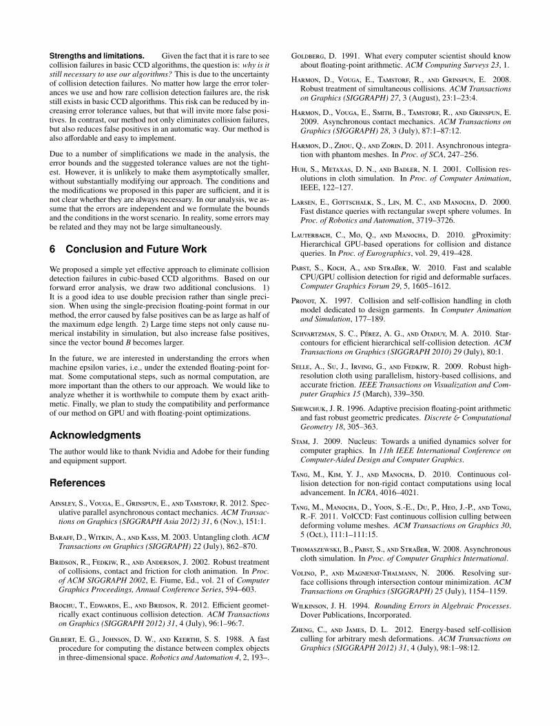
(a) A lifted tablecloth (b) Colliding tablecloth (c) Virtual clothing

Figure 7: Animation examples. These are the examples used to test the performance and robustness of our system.

based culling by introducing another error tolerance. To furtherspeed up our algorithms, we developed another culling method forthe vertex-edge test. Specifically, given the computed collision timecandidate t0, we first test whether the magnitude of the cubic func-tion value goes beyond µ at both t0 ± ε

12 . If so, when collision hap-

pens at t0, we must have |t0−t0| ≤ ε12 . Given B as an upper bound on

the relative velocities, the distance between the vertex’s projectionand the triangle must be bounded by

√3Bε

12 at time t0, and at least

one barycentric weight must be in [−9B4ε12 , ||N||22 +9B4ε

12 ]. In other

words, no collision can happen if the weight is beyond this range.Since ε is small, this test can eliminate more than 99.9 percent ofVE tests as our experiment shows.

One issue we have not considered yet is the errors in vector com-putation. Take vertex-vertex CCD for example. The goal is to findthe collision between {x0

i , x1i } and {x0

j , x1j }, but the algorithm tests

{x0i , x

1i } and {x0

i + x ji, x1i + x ji + v ji}. Since such errors are bounded

by BO(ε), if a collision failure happens because of this, the vertex-triangle distance at the ending time must be bounded by BO(ε).This problem can be solved by doing proximity tests at the endingtime as in many existing systems, including ours. Since our toler-ances are larger, they guarantee the detection of such collisions.

Another issue comes from the upper bound B, when it is computedfor every time step. Let B0 be the upper bound in the previous timestep and B1 be the upper bound in the next time step. If B1 > B0,collisions may be detected at the starting time of the next step, caus-ing convergence issues in collision handling. One possible solutionis to go back to the previous time step and use B1 for collision detec-tion at the ending time. For simplicity, we predefine B and assumethat it is valid through the whole animation. We can even defineB separately for every vertex-triangle or edge-edge pair, using theirresting shapes. Doing this reduces B, when handling adaptivelysampled meshes with both long and short edges.

Performance. We first test the performance of our algorithm-s on four cloth animation examples as shown in Figure 1 and 7,using a single core of a 2.67GHz Intel Xeon X5650 processor. Af-ter AABB culling, the average computational time of each basicvertex-triangle or edge-edge CCD test is 350ns, while the computa-tional time after using our modifications is 355ns. So the overheadis approximately 1.4 percent of the basic cost. Without plane-basedculling, the costs before and after our modifications are 409ns and416ns. To better understand the performance in complex situations,we construct a synthetic example by randomly sampling vertex po-sitions and velocities in a unit cube and we exhaustively tested 10billion cases (taking about one hour to run). The average compu-tational costs per test before and after our modifications are 364nsand 369ns. The timing difference between the synthetic exampleand the animation examples is due to more positive cases.

Compared with the exact approach proposed by Brochu and Brid-son [2012], our tests run 20 to 40 times faster than exact tests aftercollision culling. This is highly noticeable in the synthetic exam-ple, where nearly half cases pass AABB culling and nearly onethird cases pass plane-based culling. Our experiment shows the av-erage time per exact test is 4,962ns after AABB culling. In contrast,our tests are fast even without culling. In real animation examples,however, such difference may not be so noticeable because of col-lision culling. The only difference we found occurs at the collisionpeaking time, when our approach can be up to 20 percent faster thanthe exact approach. We believe the efficiency of our approach willbe more obvious, once the cost of collision culling becomes lessdominant in the overall collision handling cost.

False positives. According to our previous analysis, the max-imum vertex-triangle (or edge-edge) distance of a false positive isapproximately 20µm in our simulation. To evaluate the influenceof false positives on animation examples, we cannot simply countthem among all of the positive cases, because a false positive mayjust cause earlier collision handling and avoid true positives fromhappening later. So instead, we count the total numbers of testedcases and their positive results, when we simulate the animationexamples using our approach and the exact approach respective-ly. Our experiment shows that the total case numbers are about thesame when using the two approaches, but the system can detect upto 10 percent more positive cases when using our approach. For-tunately, since most results are negative, these additional positiveshave little influence on the collision detection performance.

Safety. Collision detection failures can be problematic incubic-based CCD tests, if no error tolerance is used. Even when tol-erances are used, it is still possible to construct failure cases basedon the two degenerate cases as shown in Subsection 3.3. Inter-estingly, it is extremely rare to see failures in cloth animation andthe colliding cloth example in Figure 7b is the only failure one wefound. In this example, basic CCD tests missed multiple collisionsat first. Shortly after that, a burst of collisions were detected andcollision handling failed to converge. We did not apply other tech-niques (such as impact zones) to fix it after this. We believe that col-lision failures are rare in cloth animation due to two main reasons.The first reason is because physically based simulation often avoid-s small triangle or short edge cases for numerical stability. If weassume that the triangle areas and the edge lengths remain approxi-mately constant, then we can reduce the error bounds substantially.The second reason is that the failure of a single case does not nec-essarily cause the failure of the whole collision handling process.For instance, ill-shaped triangles or edges may be surrounded bygood-shaped ones, whose correct test results will prevent failuresfrom happening. It will be interesting to see whether basic CCDtests are more likely to fail in other cases, such as hair animation.

Strengths and limitations. Given the fact that it is rare to seecollision failures in basic CCD algorithms, the question is: why is itstill necessary to use our algorithms? This is due to the uncertaintyof collision detection failures. No matter how large the error toler-ances we use and how rare collision detection failures are, the riskstill exists in basic CCD algorithms. This risk can be reduced by in-creasing error tolerance values, but that will invite more false posi-tives. In contrast, our method not only eliminates collision failures,but also reduces false positives in an automatic way. Our method isalso affordable and easy to implement.

Due to a number of simplifications we made in the analysis, theerror bounds and the suggested tolerance values are not the tight-est. However, it is unlikely to make them asymptotically smaller,without substantially modifying our approach. The conditions andthe modifications we proposed in this paper are sufficient, and it isnot clear whether they are always necessary. In our analysis, we as-sume that the errors are independent and we formulate the boundsand the conditions in the worst scenario. In reality, some errors maybe related and they may not be large simultaneously.

6 Conclusion and Future Work

We proposed a simple yet effective approach to eliminate collisiondetection failures in cubic-based CCD algorithms. Based on ourforward error analysis, we draw two additional conclusions. 1)It is a good idea to use double precision rather than single preci-sion. When using the single-precision floating-point format in ourmethod, the error caused by false positives can be as large as half ofthe maximum edge length. 2) Large time steps not only cause nu-merical instability in simulation, but also increase false positives,since the vector bound B becomes larger.

In the future, we are interested in understanding the errors whenmachine epsilon varies, i.e., under the extended floating-point for-mat. Some computational steps, such as normal computation, aremore important than the others to our approach. We would like toanalyze whether it is worthwhile to compute them by exact arith-metic. Finally, we plan to study the compatibility and performanceof our method on GPU and with floating-point optimizations.

AcknowledgmentsThe author would like to thank Nvidia and Adobe for their fundingand equipment support.

References

Ainsley, S., Vouga, E., Grinspun, E., and Tamstorf, R. 2012. Spec-ulative parallel asynchronous contact mechanics. ACM Transac-tions on Graphics (SIGGRAPH Asia 2012) 31, 6 (Nov.), 151:1.

Baraff, D., Witkin, A., andKass, M. 2003. Untangling cloth. ACMTransactions on Graphics (SIGGRAPH) 22 (July), 862–870.

Bridson, R., Fedkiw, R., and Anderson, J. 2002. Robust treatmentof collisions, contact and friction for cloth animation. In Proc.of ACM SIGGRAPH 2002, E. Fiume, Ed., vol. 21 of ComputerGraphics Proceedings, Annual Conference Series, 594–603.

Brochu, T., Edwards, E., and Bridson, R. 2012. Efficient geomet-rically exact continuous collision detection. ACM Transactionson Graphics (SIGGRAPH 2012) 31, 4 (July), 96:1–96:7.

Gilbert, E. G., Johnson, D. W., and Keerthi, S. S. 1988. A fastprocedure for computing the distance between complex objectsin three-dimensional space. Robotics and Automation 4, 2, 193–.

Goldberg, D. 1991. What every computer scientist should knowabout floating-point arithmetic. ACM Computing Surveys 23, 1.

Harmon, D., Vouga, E., Tamstorf, R., and Grinspun, E. 2008.Robust treatment of simultaneous collisions. ACM Transactionson Graphics (SIGGRAPH) 27, 3 (August), 23:1–23:4.

Harmon, D., Vouga, E., Smith, B., Tamstorf, R., and Grinspun, E.2009. Asynchronous contact mechanics. ACM Transactions onGraphics (SIGGRAPH) 28, 3 (July), 87:1–87:12.

Harmon, D., Zhou, Q., and Zorin, D. 2011. Asynchronous integra-tion with phantom meshes. In Proc. of SCA, 247–256.

Huh, S., Metaxas, D. N., and Badler, N. I. 2001. Collision res-olutions in cloth simulation. In Proc. of Computer Animation,IEEE, 122–127.

Larsen, E., Gottschalk, S., Lin, M. C., and Manocha, D. 2000.Fast distance queries with rectangular swept sphere volumes. InProc. of Robotics and Automation, 3719–3726.

Lauterbach, C., Mo, Q., and Manocha, D. 2010. gProximity:Hierarchical GPU-based operations for collision and distancequeries. In Proc. of Eurographics, vol. 29, 419–428.

Pabst, S., Koch, A., and Straßer, W. 2010. Fast and scalableCPU/GPU collision detection for rigid and deformable surfaces.Computer Graphics Forum 29, 5, 1605–1612.

Provot, X. 1997. Collision and self-collision handling in clothmodel dedicated to design garments. In Computer Animationand Simulation, 177–189.

Schvartzman, S. C., Perez, A. G., and Otaduy, M. A. 2010. Star-contours for efficient hierarchical self-collision detection. ACMTransactions on Graphics (SIGGRAPH 2010) 29 (July), 80:1.

Selle, A., Su, J., Irving, G., and Fedkiw, R. 2009. Robust high-resolution cloth using parallelism, history-based collisions, andaccurate friction. IEEE Transactions on Visualization and Com-puter Graphics 15 (March), 339–350.

Shewchuk, J. R. 1996. Adaptive precision floating-point arithmeticand fast robust geometric predicates. Discrete & ComputationalGeometry 18, 305–363.

Stam, J. 2009. Nucleus: Towards a unified dynamics solver forcomputer graphics. In 11th IEEE International Conference onComputer-Aided Design and Computer Graphics.

Tang, M., Kim, Y. J., and Manocha, D. 2010. Continuous col-lision detection for non-rigid contact computations using localadvancement. In ICRA, 4016–4021.

Tang, M., Manocha, D., Yoon, S.-E., Du, P., Heo, J.-P., and Tong,R.-F. 2011. VolCCD: Fast continuous collision culling betweendeforming volume meshes. ACM Transactions on Graphics 30,5 (Oct.), 111:1–111:15.

Thomaszewski, B., Pabst, S., and Straßer, W. 2008. Asynchronouscloth simulation. In Proc. of Computer Graphics International.

Volino, P., and Magnenat-Thalmann, N. 2006. Resolving sur-face collisions through intersection contour minimization. ACMTransactions on Graphics (SIGGRAPH) 25 (July), 1154–1159.

Wilkinson, J. H. 1994. Rounding Errors in Algebraic Processes.Dover Publications, Incorporated.

Zheng, C., and James, D. L. 2012. Energy-based self-collisionculling for arbitrary mesh deformations. ACM Transactions onGraphics (SIGGRAPH 2012) 31, 4 (July), 98:1–98:12.