Deep-water subsurface imagingusing OBS interferometry

Olivier Carrière1 and Peter Gerstoft1

ABSTRACT

Seismic interferometry processing is applied to an activeseismic survey collected on ocean bottom seismometers(OBS) deployed at 900-m water depth over a carbonate/hydrates mound in the Gulf of Mexico. Common midpointprocessing and stacking of the extracted Green’s functiongives the subsurface PP reflectivity, with a horizontal reso-lution of half the receiver spacing. The obtained seismicsection is comparable to classical upgoing/downgoingwavefield decomposition and deconvolution applied on acommon receiver gather. Seismic interferometry does notrequire precise knowledge of source geometry or shootingtimes, but more accurate results are obtained when includingthis information for segmenting the signals before the cross-correlations, especially when signals from distant surveysare present in the data. Reflectivity estimates can be obtainedwith the crosscorrelation of pressure or vertical particlevelocity signals, but the pressure data gives the best resolu-tion due to the wider frequency bandwidth and the reducedamount of noise bursts.

INTRODUCTION

The study and monitoring of complex natural marine hydratesrequire long-term or periodic data collection. For this purpose, datacollected from long-term deployment of ocean-bottom seism-ometers (OBS) can be used for detecting and monitoring changesin hydrate distribution and other hydrocarbon related subsurfaceprocess. In this paper, empirical Green’s functions are extractedfrom crosscorrelated signals collected over a 2D transect ofOBS. Results are used to estimate seismic reflectivity of the shallowsubsurface.Data were acquired at Woolsey Mound, a very active carbonate/

hydrates structure in Mississippi Canyon Lease Block 118 (MC118),

Northern Gulf of Mexico, used as seafloor observatory by theHydrates Research Consortium for more than a decade (McGeeet al., 2009). The mound is about 1 km in diameter and locatedin nearly 900-m water depth. Recent study of the mound subsurfaceintegrating several seismic data sets at different resolutions(backscatter, autonomous underwater vehicle [AUV], and shallowsource/deep receiver [SSDR] surveys) has shown that the mound isformed by crestal normal faults nucleating at the top of a diapir-shaped salt body present in the shallow subsurface (Macelloni et al.,2012). The OBS transect used here crosses one of the main normalfaults of the mound.The measurement of pressure and particle velocity, as provided

by multicomponent OBS, give access to the upgoing and down-going wavefields (Schneider and Backus, 1964; Loewenthal et al.,1985; Amundsen and Reitan, 1995; Schalkwijk et al., 1999). Indeep-water, when the target zone is within a few hundred metersof the seafloor, surface multiples arrive much later than primary re-flections of interest, and the wavelet estimation follows directlyfrom the upgoing/downgoing decomposition (Backus et al.,2006). Such a technique enables high-resolution images. As forother conventional seismic processing methods, this approach re-quires the knowledge of the shooting times and associatedsource-receiver geometry. Multicomponent acquisition gives alsoaccess to the shear reflectivity of the subsurface which is relevantfor hydrates assessment (Backus et al., 2006).As conjectured by Rickett and Claerbout (1999), and as demon-

strated in many areas (helioseismology, ultrasounds, seismics,ocean acoustics, etc.) crosscorrelations of signals recorded ontwo distinct receivers enables the estimation of the Green’s functionbetween these two receivers, without knowledge of source positionand wavelet. In seismics, Green’s function extraction from cross-correlations is referred to as “seismic interferometry” (Schuster,2009). When applied to a controlled source survey, seismic inter-ferometry is a redatuming process in which the redatum operator isdeduced directly from the data, i.e., no velocity model is required,which is attractive when a complex structure overlies the targets(Bakulin and Calvert, 2006). Different crosscorrelation-based

Manuscript received by the Editor 26 June 2012; revised manuscript received 26 October 2012.1University of California, Marine Physical Laboratory, Scripps Institution of Oceanography, San Diego, California, USA. E-mail: ocarriere@ucsd.edu;

gerstoft@ucsd.edu.© 2012 Society of Exploration Geophysicists. All rights reserved.

1

GEOPHYSICS, VOL. 78, NO. 2 (MARCH-APRIL 2013); P. 1–10, 13 FIGS.10.1190/GEO2012-0241.1

methods exist and essentially differ in the weighting of the cross-correlations (Schuster and Zhou, 2006).Seismic interferometry has become very popular since the 2000s

with the mathematical proof of daylight imaging (Wapenaar et al.,2002; Schuster et al., 2004; Wapenaar, 2004). Many passive appli-cations have been proposed, such as earthquake coda interferometry(Snieder et al., 2002; Shapiro and Campillo, 2004), surface-wavetomography (Shapiro et al., 2005; Gerstoft et al., 2006), body-waves interferometry (Roux et al., 2005; Miyazawa et al., 2008),or interferometric reflection seismics (Draganov et al., 2007). Aspecial section of GEOPHYSICS edited byWapenaar et al. (2006) drawsup a comprehensive review of seismic interferometry history andapplications. Wapenaar et al. (2010a) and Wapenaar et al.(2010b) give an updated review of seismic interferometry theoryand its recent progresses.The interest of active seismic interferometry for exploration has

been demonstrated for vertical seismic profiling (Bakulin andCalvert, 2006; Vasconcelos et al., 2008), inverse vertical seismicprofiling (Yu and Schuster, 2006), and crosswell data (Minato et al.,2011). A few papers also deal with OBS or OBC (ocean-bottomcable) data: Mehta et al. (2007) demonstrated the improvementof virtual source technique (Bakulin and Calvert, 2006) by decom-posing the wavefield acquired on deep-water OBC data; elasticinterferometry theory was proposed by Gaiser and Vasconcelos(2009) and applied on OBC data in shallow water for retrievingP-waves and P-to-S waves using refraction interferometry (Donget al., 2006), Bharadwaj et al. (2012) generated supervirtual traceson OBS to increase signal-to-noise ratio (S/N) and facilitate thetraveltime picking of far-offset traces and head waves. Haines(2011) applied interferometric processing to a deep-water OBS dataset, using a large OBS array (160 elements spanning 4 km), for thepurpose of shallow subsurface imaging (<500 m). However, theprocessing was restricted to single receiver interferometry (cross-correlation of different wavefields received on a single OBS)instead of crosscorrelating pairs of receivers. Here, deep-waterOBS data are interferometrically redatumed followed by a mod-el-based time-migration assuming horizontal layering and specularreflections. Signals are crosscorrelated between pairs of OBS andonly PP reflections are considered. The obtained image is found tobe comparable to a conventional image (using an upgoing/down-going decomposition) from the same OBS data set but with areduced horizontal resolution. In both methods, the processing isrestricted to primary reflections. When applicable, the processingof surface multiples has been demonstrated to broaden illuminationand increase horizontal resolution (Jiang et al., 2005; Dash et al.,2009). As horizontal propagation dominates ambient noise, the ef-fective use of multiples has not been demonstrated yet in a purelypassive approach. Moreover, the strong interferences from a distantseismic survey (see below) prevent here the use of multiples onmany received shots.With suitable noise field characteristics, the interferometric

approach can be extended to ambient noise (or passive) processing.Passive monitoring typically requires longer acquisition time toaccumulate sufficient energy along the stationary-phase pathsand averaging down possible dominant but unwanted arrivals thatbias the noise distribution. Given the increasing availability of re-ceivers, this enables long-term passive seismic monitoring, thussuppressing the need for an active survey. Passive reflectivity ima-ging with OBC was proposed by Hohl and Mateeva (2006), but the

results were not conclusive because of too short an observationtime. At lower frequencies (0.35–1.75 Hz, the double-frequency mi-croseismic band), de Ridder and Dellinger (2011) demonstratedpassive interferometric imaging of Scholte-wave velocities usinga few hours of data. Using local earthquakes, Minato et al.(2012) localize the oceanic crust surface using a 3D array of28 OBS. Due to the localized nature of the sources, they proposeto exclude receiver pair that do not correspond to stationary-phasepaths to improve the imaging results. Harmon et al. (2007) and Yaoet al. (2011) invert for shear-velocity structure in the crust anduppermost mantle using dispersion of Scholte-Rayleigh waveempirical Green’s functions extracted from long-term (∼1 year)recording on OBS. Interferometric processing at these low frequen-cies (0.01–1 Hz) requires large OBS offsets, typically tens or hun-dreds of kilometers. Low-frequency passive interferometry can alsobe useful for correcting the time drift of OBS, as proposed byHatchell and Mehta (2010). In our case, only a single day of con-tinuous passive monitoring was available from the April 2011MC118 experiment. Unfortunately, distant seismic explorationdominates the noise sequence from a single direction and requiresfurther processing before assessing the potential use of ambientnoise for shallow subseafloor imaging. Therefore, we do not pursueinterferometric imaging based on this passive data set and use theavailable active data set as a proxy for passive data processing.The remainder of the paper is as follows: The next section details

the OBS data set acquired at the Woolsey Mound and illustrates theprincipal reflectivity properties of the subsurface deduced from pre-vious surveys. Then the OBS data from one of the endfire surveysare processed with a conventional upgoing/downgoing seismic pro-cessing. Next the same active data are processed using an interfero-metric approach. The same section then discusses how passive datawould be interferometrically processed, compared to the present ac-tive interferometric processing.

OBS DATA

In April 2011, 15 OBS provided by Woods Hole OceanographicInstitution were deployed at the Woolsey Mound (Northern Gulf ofMexico) at 900-m water depth for a few days. The OBS weredropped from the sea surface and afterward the precise locationwas surveyed. These locations are used here. The OBS formed aline array with 11 OBS nominally spaced 25 m apart and2 OBS spaced 500 m apart on each side, giving a total apertureof 2250 m (Figure 1). A gas-injection (GI) gun was towed nearthe surface above the OBS line, from south to north, shooting every25 m covering 5500 m range. The active OBS survey was per-formed on April 7, from 10:01 to 11:03 UTC, resulting in a newshot every 10–15 s triggered manually due to computer failure.A crossfire active survey (west–east) and watergun shooting onthe same day complete the data set but are not discussed.The OBS signals can be combined through array processing to

separate signals that have overlapping frequency content but origi-nate from different azimuths, using a plane-wave beamformingprocessor (Van Veen and Buckley, 1988). Figure 2 shows theplane-wave beamformer output for the acoustic energy receivedat 30 Hz using the closely spaced OBS (OBS 1 to 11) aroundthe period of the south-to-north survey. As the array is linear(1D), the beamformer output has an cylindrical symmetry aroundthe array axis. Therefore, the resolved angle is usually termed “coneangle”. When an acoustic source is at large range, this angle is the

2 Carrière and Gerstoft

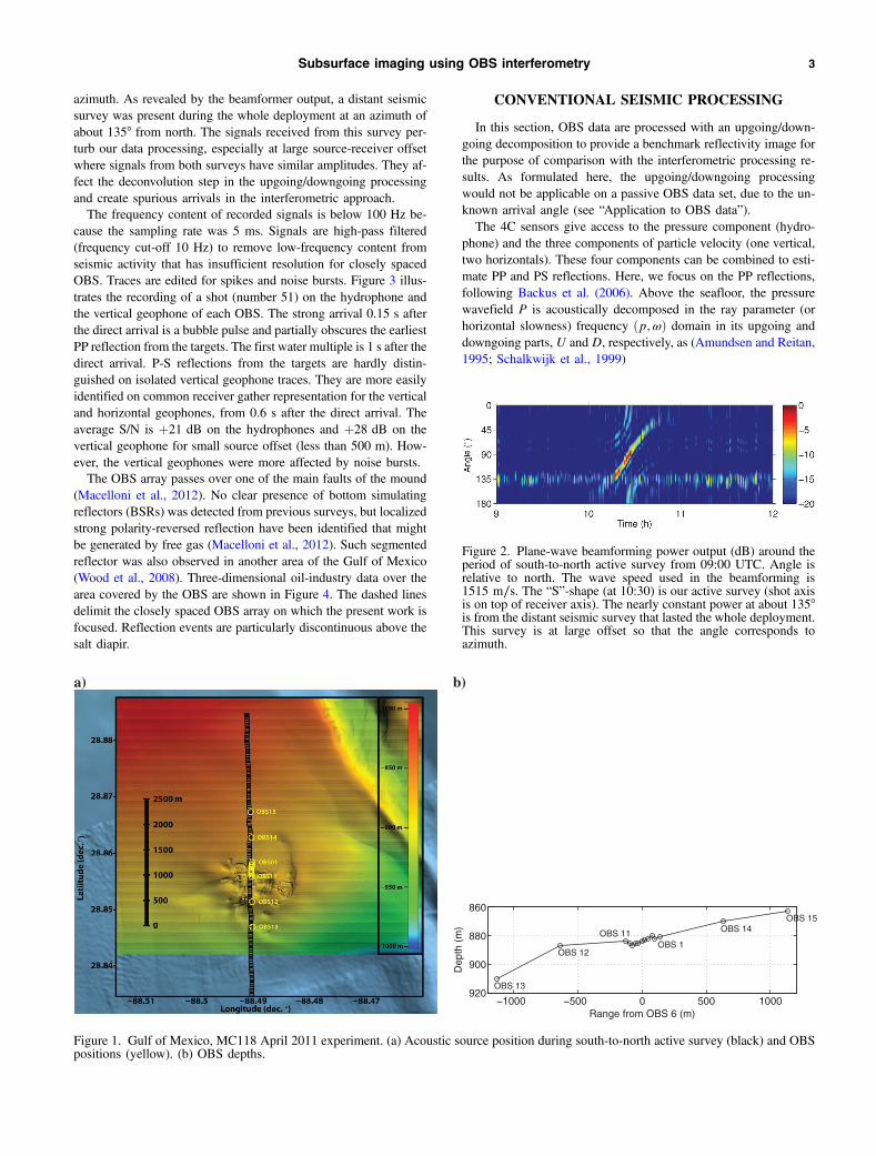
azimuth. As revealed by the beamformer output, a distant seismicsurvey was present during the whole deployment at an azimuth ofabout 135° from north. The signals received from this survey per-turb our data processing, especially at large source-receiver offsetwhere signals from both surveys have similar amplitudes. They af-fect the deconvolution step in the upgoing/downgoing processingand create spurious arrivals in the interferometric approach.The frequency content of recorded signals is below 100 Hz be-

cause the sampling rate was 5 ms. Signals are high-pass filtered(frequency cut-off 10 Hz) to remove low-frequency content fromseismic activity that has insufficient resolution for closely spacedOBS. Traces are edited for spikes and noise bursts. Figure 3 illus-trates the recording of a shot (number 51) on the hydrophone andthe vertical geophone of each OBS. The strong arrival 0.15 s afterthe direct arrival is a bubble pulse and partially obscures the earliestPP reflection from the targets. The first water multiple is 1 s after thedirect arrival. P-S reflections from the targets are hardly distin-guished on isolated vertical geophone traces. They are more easilyidentified on common receiver gather representation for the verticaland horizontal geophones, from 0.6 s after the direct arrival. Theaverage S/N is !21 dB on the hydrophones and !28 dB on thevertical geophone for small source offset (less than 500 m). How-ever, the vertical geophones were more affected by noise bursts.The OBS array passes over one of the main faults of the mound

(Macelloni et al., 2012). No clear presence of bottom simulatingreflectors (BSRs) was detected from previous surveys, but localizedstrong polarity-reversed reflection have been identified that mightbe generated by free gas (Macelloni et al., 2012). Such segmentedreflector was also observed in another area of the Gulf of Mexico(Wood et al., 2008). Three-dimensional oil-industry data over thearea covered by the OBS are shown in Figure 4. The dashed linesdelimit the closely spaced OBS array on which the present work isfocused. Reflection events are particularly discontinuous above thesalt diapir.

CONVENTIONAL SEISMIC PROCESSING

In this section, OBS data are processed with an upgoing/down-going decomposition to provide a benchmark reflectivity image forthe purpose of comparison with the interferometric processing re-sults. As formulated here, the upgoing/downgoing processingwould not be applicable on a passive OBS data set, due to the un-known arrival angle (see “Application to OBS data”).The 4C sensors give access to the pressure component (hydro-

phone) and the three components of particle velocity (one vertical,two horizontals). These four components can be combined to esti-mate PP and PS reflections. Here, we focus on the PP reflections,following Backus et al. (2006). Above the seafloor, the pressurewavefield P is acoustically decomposed in the ray parameter (orhorizontal slowness) frequency "p;ω# domain in its upgoing anddowngoing parts, U and D, respectively, as (Amundsen and Reitan,1995; Schalkwijk et al., 1999)

!1000 !500 0 500 1000

860

880

900

920

Range from OBS 6 (m)

Dep

th (

m)

OBS 13

OBS 12

OBS 11OBS 1

OBS 14OBS 15

a) b)

Figure 1. Gulf of Mexico, MC118 April 2011 experiment. (a) Acoustic source position during south-to-north active survey (black) and OBSpositions (yellow). (b) OBS depths.

Figure 2. Plane-wave beamforming power output (dB) around theperiod of south-to-north active survey from 09:00 UTC. Angle isrelative to north. The wave speed used in the beamforming is1515 m∕s. The “S”-shape (at 10:30) is our active survey (shot axisis on top of receiver axis). The nearly constant power at about 135°is from the distant seismic survey that lasted the whole deployment.This survey is at large offset so that the angle corresponds toazimuth.

Subsurface imaging using OBS interferometry 3

U"p;ω; z# $ 1

2

!P"p;ω; z# −Hcal"ω# ρ"z#

q"z#Vz"p;ω; z#

"

(1)

D"p;ω; z# $ 1

2

!P"p;ω; z# !Hcal"ω# ρ"z#

q"z#Vz"p;ω; z#

";

(2)

where P"p;ω; z# and Vz"p;ω; z# are the pressure and the verticalparticle velocity, ρ"z# is the density, and q"z# is the vertical ray para-meter (or vertical slowness) defined by

q"z# $#######################c"z#−2 − p2

q; (3)

where c"z# is the sound speed in water. The factorHcal calibrates thevertical geophone to the hydrophone. Backus et al. (2007) demon-strated that a frequency-dependent sensor calibration was necessaryonly for the recovery of calibrated reflectivity in the shallow depthsimmediately below the seafloor (a few tens of meters) whereas con-stant gain factor provided accurate results for deeper reflections.Here, for each given OBS, a cross-equalization filter (Wiener filter)averaged over all traces provided an adequate calibration factorHcal

that enables satisfactory up/down separation. Nevertheless, no sig-nificant reflectivity difference was found between such a frequency-dependent calibration and a constant gain factor for the targets ofinterest (∼200 m below the seafloor).This decomposition is only valid just above the seafloor (no

shear). Strictly speaking, the estimate of P- and S-wave componentsbelow the seafloor requires an elastic decomposition using P- and S-wave velocity and density below the receiver (Amundsen and Re-itan, 1995; Schalkwijk et al., 1999). However, an acoustic decom-position is sufficient for imaging shallow subsurface PP and PSreflection events in deep-water (Backus et al., 2007).Equation 2 is associated with the downgoing seismic wavelet.

The PP reflectivity R is estimated from the spectral division ofthe upgoing wavefield U with the downgoing wavelet D (Loe-wenthal et al., 1985; Amundsen, 2001):

R $ D%UD%D! ϵ

; (4)

where ϵ is a positive stabilization term and * denotes the conjugate.The reflectivity is related to the impedance contrast in the medium,and thus density and sound speed changes.The deconvolution (equation 4) removes the source signature ef-

ficiently (wavelet and associated bubbles) and redatums the shots tothe receiver datum on the seafloor. Surface multiples do not requirea specific processing because they appear much later than the tar-geted events. The seafloor redatuming is important for the BSR de-tection, because the BSR tends to be parallel to the seafloor andtherefore would appear as a straight-line event after redatuming.For the same reason, seafloor redatuming helps identify unconfor-mities.Equations 1–4 are applied independently to each common recei-

ver gather (CRG). Figure 5a illustrates the resulting time-domain PPreflectivity for one receiver (OBS 3). Curved events are typicallyrelated to reflection events whereas horizontal events related to di-rect arrivals are removed by the deconvolution. The strong noiselevel on the resulting CRG is explained by signal corruption onthe vertical geophone, but also due to another seismic explorationsignals that perturb the upgoing/downgoing decomposition and de-convolution. The complex subsurface structure could explain dis-continuities in the reflection curves.The moveout is corrected using a ray-tracing model, assuming a

four-layer subsurface model with a piecewise increasing P-wavevelocity (1550, 1600, 1750, and 2000 m∕s), with subsurface inter-faces at depth 85, 150, and 470 m. This model gives the observed

0 0.5 1 1.5 2 2.5 3

OBS13

OBS12

OBS11

OBS10

OBS09

OBS08

OBS07

OBS06

OBS05

OBS04

OBS03

OBS02

OBS01

OBS14

OBS15

Time (s)

Figure 3. Shot number 51. Normalized pressure (black) and verticalparticle velocity (gray) signals on the OBS elements during south-to-north active survey. The source is near vertical incidence for OBS13. OBS 1–OBS 11 have 25-m spacing. OBS 12, 13, 14, and 15 are500-m apart (see Figure 1).

TW

T (

s)

South!North range (trace #)50 100 150 200

1

1.2

1.4

1.6

1.8

2

2.2

Figure 4. PP reflectivity estimated from proprietary deep seismicdata, sea-level datum. The closely spaced OBS array position(OBS 1–OBS11, between the dashed lines) corresponds to thetop of the salt dome. Inside this region, most of the reflectionsare discontinuous. A strong negative (blue) event is identifiedaround 1.4 s (0.2 s below seabottom reflection). (Courtesy ofWesternGeco).

4 Carrière and Gerstoft

two-way traveltimes (TWT) of 0.1, 0.2, and 0.55 s in the near-offsettraces. The velocity range is similar to the P-wave velocity model ob-tained nearby by Murray and DeAngelo (2008), but does not considerany velocity drop that would be caused by free gas. The moveoutcorrection reasonably flattens the reflection curves (see Figure 5b).The geometry of acquisition (near-surface source, sea bottom re-

ceivers) makes the actual reflection points depth-dependent, even in ahorizontally stratified environment. Therefore, the CRG data have tobe converted to common depth point (CDP) gather. Theoreticalcurves of source-receiver offset versus time for reflection depthpoints at specified offsets from the receiver location are calculatedusing ray tracing (black lines in Figure 5b). CDP data are recoveredby interpolation along these curves. Here, offset curves between&−100; 100' mwith a 5-m spacing are retrieved for each CRG, givinga 5-m horizontal resolution for the whole section. The CDP data arestacked to improve the S/N. The chosen offset of (100 m implies aminimum of five folds for the subseafloor section delimited by theOBS array and keeping a weak dependence to the velocity model. Amaximum number of nine folds is achieved in the center of the array.The upgoing/downgoing decomposition and deconvolution give

a reasonable estimate of the PP reflectivity beneath the sectioncovered by the closely spaced OBS, see Figure 6. Although the de-convolution operator is not optimal due to calibration issues, inter-ferences from distant seismic exploration, and possible tilt ofvertical geophones not accounted for (Li et al., 2004). Comparedto the deep seismic data (Figure 4), the same three principal inter-faces are well identified at 0.1, 0.2, and 0.55 s. The second reflectorhas a negative polarity, which might indicate the base of the hydratestability zone (BHSZ). The third reflector most likely correspondsto the top of the salt dome identified in the deep seismic data ac-quired on a larger zone at the same location (Figure 4). This reflec-tor is here continuous over the whole section whereas deep seismicdata exhibit a discontinuity at the middle of the section. Overall,reflectors exhibit fewer discontinuities in OBS data. This differencemight be reinforced by the datum difference (sea-level datum for the

deep seismic data and seafloor datum for the OBS data) but is likelydue to lack of horizontal resolution in the OBS data. No relevantreflections are detected below the third reflector (not shown).

GREEN’S FUNCTION EXTRACTION

Theory

Theoretically, the Green’s function between two given points canbe extracted by crosscorrelating waves recorded at these two pointsand excited by sources distributed on a closed surface around (see,e.g., Wapenaar, 2004). In the seismic community, Green’s functionextraction is better known as seismic interferometry. In most experi-mental configurations, receivers are typically not fully surroundedby sources and the latter are often located on a single side of thereceiver pair. As demonstrated (Snieder et al., 2006; Brooks andGerstoft, 2007), the lack of a closed surface for the source locationsleads to artifacts in the reconstructed Green’s function (spurious ar-rivals). This effect is reduced when the medium is sufficiently het-erogenous (Wapenaar, 2006). For controlled sources (active data), apractical way to reduce spurious arrivals is isolating the direct arri-val on one of the signals before crosscorrelation (Sheley and Schus-ter, 2003; Yu and Schuster, 2006; Mehta et al., 2007).Considering a set of sources that are distributed over a horizontal

line, the crosscorrelation of waves received on receivers A and B isgiven in the frequency domain by (Snieder et al., 2006)

CAB"ω# $ jS"ω#j2nZ

G"rA; rs#G%"rB; rs#drs; (5)

where G"ri; rs# denotes the Green’s function between receiver i atri and source at rs, S"ω# is the source spectrum, and n is the numberof sources per unit length. The integral in equation 5 gives the ap-proximated Green’s function G"rA; rB# (Sabra et al., 2005; Sniederet al., 2006; Brooks and Gerstoft, 2007, 2009a).

!2 !1 0 1 2

0

0.2

0.4

0.6Red

uced

TW

T (

s)

!2 !1 0 1 2

0

0.2

0.4

0.6

Source offset (km)

Red

uced

TW

T (

s)

a)

b)

!0.1

!0.05

0

0.05

0.1

0.15

Figure 5. (a) Time-domain PP reflectivity estimate for OBS 3.(b) Moveout correction based on flat-layered earth model and anincreasing P-wave velocity. The theoretical curves of source-receiver offset versus time for reflection depth points at receiveroffsets (5 m, (25 m, (50 m, (75 m, and (100 m are shown(black lines).

!100 !50 0 50

0

0.1

0.2

0.3

0.4

0.5

0.6

Range from OBS 6 (m)

Red

uced

TW

T (

s)

0

100

200

300

400

500

Dep

th (

m @

1750

m/s

)

!0.1

!0.05

0

0.05

0.1

0.15

Figure 6. PP reflectivity obtained with conventional seismic pro-cessing (seafloor datum).

Subsurface imaging using OBS interferometry 5

With the sources being distributed over a horizontal line, the ex-act phase dependence of the extracted Green’s function is obtainedthrough a Hilbert transform and a fractional derivative of CAB(Snieder et al., 2006). Exact amplitude retrievals require reflectioncoefficients, path-dependent coefficients, and source spectrumterms, and are usually ignored. Therefore, the Green’s functionextraction from equation 5 enables the estimate of the reflector po-sitions but cannot estimate their strength.The active source is ∼2 m below the sea surface and the towing

trajectory roughly aligned to the receivers. Therefore, we only con-sider the stationary-phase points distributed along the receiver axis.Four kinds of contributing paths are distinguished, as illustrated inFigure 7. Type a is related to the direct arrival and involves noreflection. Type b involves first a reflection before reaching thereceivers successively. Type c corresponds to a wave that encountersa reflection along the propagation between the two receivers. Type dexists for the multiple reflector case. Note that this type d does notcorrespond to a physical arrival between the receivers and wouldthen be an artifact in the extracted Green’s function.Here, the receivers are considered at the same depth (see Fig-

ure 1b). The finite source offset makes that the stationary-phasepoint related to the direct arrival (type a) or reflected arrival (typeb) is never reached, leaving only type c and d as precisely deter-mined by the interferometric approach. Neglecting refraction, thesource position giving stationary-phase path (type c) of a singlespecular reflection (assuming horizontal layering) is determinedgeometrically. Given a receiver spacing of r, water depth D, andreflector at depth H below the seafloor, the offset rst of the station-ary-phase point is (Figure 8)

rst $rD2H

: (6)

Therefore, considering a maximum source-receiver offsetrst $ 2500 m, the minimum reflector depth resolved, H, increaseslinearly with receiver spacing r (H ≈ 5 m with r $ 25-m receiver

spacing, H ≈ 50 m with r $ 250-m receiver spacing). This meansthat sensors separated by r $ 500 m are not able to image a reflec-tor located at less than H $ 100 m below the seafloor.On the other hand, a larger receiver spacing is expected to in-

crease the accuracy of deep reflector localization (ignoring sig-nal-to-noise ratio issues). Considering two reflectors at depths Hand H ! Δh, the source offset difference between their respectivestationary-phase paths is (for Δh ≪ H)

Δr $ rst;H!Δh − rst;H $ rD2"H ! Δh#

−rD2H

≈ −rD2H2

Δh:

(7)

The H2 term is critical. Keeping shot spacing Δr (and water depthD) fixed, to maintain the same resolution Δh at a depth H $ 500 mas at H $ 50 m, requires the receiver spacing r to be increased by afactor 102 $ 100. With our limited array aperture of 250 m, theaccuracy of reflector localization at 50-m depth with 25-m receiverspacing can only be maintained up to 50 !

#####10

p≈ 150-m depth,

using the 250-m receiver spacing. For reflectors at 500-m depth,the present interferometric configuration can only localize themwith an accuracy of 50 m. The inclusion of large offset OBS thusimproves the accuracy of the deepest reflectors, but these cannotimage the shallowest reflectors, given the limited source-receiveroffset. To maintain the correspondence with upgoing/downgoingprocessing, the large offset OBS (OBS 12, 13, 14, and 15) werealso discarded in the interferometric processing.The strong bubble pulse that contaminates the signals (see Fig-

ure 3) would highly affect the crosscorrelations, resulting in a sumof shifted replica of the “true” crosscorrelation. With a bubbleoscillation period of 0.1 s, the interferometric approach is thusnot able to properly resolve the shallow subseafloor targets.Generally speaking, predictive deconvolution removes the tail ofthe wavelet (Bowen, 1986), although the very shallow reflectionsmight be lost with such approach. Here, the traces are more effi-ciently deconvolved using the downgoing wavefield estimated fromthe seismic processing (equation 2). Practically, this downgoingwavefield is time-gated for containing only the direct arrival andthe bubble pulse, resulting in an effective duration of 0.5 s. Thedeconvolution also flattens the spectrum over the processed bandby taking the factor jS"ω#j2 of equation 5 into account and com-pensates for possible variations in the source wavelet.

Reflector

Reflector

Reflector

Reflector 2

Reflector 1

a) b)

c) d)

Figure 7. Stationary-phase paths contributing to the crosscorrela-tion. The order of the arrivals between the two receivers definesthe sign of time lag in the crosscorrelation: Assuming the type(a) appears in the positive side, types (b) to (d) appear in the negativeside. For type (b) and (c), the source positions that contribute to theopposite side of the crosscorrelation are easily deduced.

Sea floor

Reflector

A B

D

H

r

rst

Figure 8. Two-dimensional geometric determination of the sourceposition (star) giving a stationary-phase path of type c for the OBSpair A-B. Seafloor and reflector are assumed horizontal. The waterdepth is D and the reflector is at depth H below the seafloor.

6 Carrière and Gerstoft

Application to OBS data

Crosscorrelations (equation 5) are computed for pressure and ver-tical particle velocity signals. The actual survey shooting times areused for segmenting the received signals. The resulting segments(3-s duration) are then crosscorrelated between a receiver pair,so that each source offset gives a crosscorrelation (crosscorrelationgather). These crosscorrelations are summed to obtain the “total”crosscorrelation (left-hand term in equation 5). The band-limited(and amplitude-shaded) empirical Green’s function are obtainedafter correcting the phase of the summed crosscorrelation. Figure 9shows the crosscorrelation gather and associated summed crosscor-relation for OBS pair three through six, for pressure and verticalparticle velocity signals. When crosscorrelating the vertical particlevelocity, care must be taken to retrieve the correct polarity of thereflection event. Pressure and vertical particle velocity have a po-sitive peak for the direct arrival, but exhibit opposite signs for pri-mary reflection peaks.Far-offset traces are typically noisier and might degrade the

crosscorrelations. Given the maximum receiver spacing considered(250 m), and the maximum reflector depth (∼500 m), crosscorrela-

tions can be done on a reduced source offset, here 1000 m, withoutaffecting the coverage of stationary-phase paths (type c in Figure 7).Due to the horizontal alignement of OBS, an infinite source offset isrequired to reach the stationary-phase paths of type a and b. Theoffset reduction thus affects the direct arrival position in the cross-correlations, but the latter is not relevant for subsurface imaging.Tapering the crosscorrelations toward the extremal values of sourceoffset reduces end-effects (Figure 9b and 9e).Figure 9d exhibits PS wave arrivals around −0.8 s and !0.7 s.

Primary PS waves propagate with a lower velocity than PP waves(shallow shear wave velocity is much lower than compressionalwave velocity). Therefore, they can be distinguished from PP wavesin the crosscorrelation gather (Figure 9d) by the late arrival time andflatter curvature of their related correlation peak trajectory (see Fig-ure 10 for justification). The asymmetry between left and right PSwaves peak trajectories is due to subsurface structure that is notperfectly horizontal as evident from CRG comparison or fromthe reflectivity image (Figure 6).If the shooting times are unknown, the signals can be crosscor-

related using a sliding overlapping time window (Figure 11a). Theuse of actual shooting time reduces the effect of other sources; in

!1 !0.8 !0.6 !0.4 !0.2 0 0.2 0.4 0.6 0.8 1!2

!1

0

1

2

Sou

rceo

ffset

(km

)

!1 !0.8 !0.6 !0.4 !0.2 0 0.2 0.4 0.6 0.8 1!0.5

00.5

Time (s)

0 1

d)

f)

e)

!1 !0.8 !0.6 !0.4 !0.2 0 0.2 0.4 0.6 0.8 1!2

!1

0

1

2

Sou

rce

offs

et(k

m)

!1 !0.8 !0.6 !0.4 !0.2 0 0.2 0.4 0.6 0.8 1!0.5

00.5

Time(s)

0 1

a)

c)

b)

Figure 9. (a) Normalized crosscorrelation gather of pressure signalson OBS 6 and 3 (75-m spacing). The source offset is relative to OBS6. Multiple-related crosscorrelation peaks appear partially at the farright and left as a negative (white) event due to the surface reflec-tion. The strong peaks at −0.05 s at large positive source offset(arrow) are due to distant survey. (b) Taper applied for removingfar-offset traces and reducing end-effects. (c) Summed crosscorre-lations after tapering. The sum is normalized and clipped at 0.5.(d-f) Same as (a-c) for the vertical particle velocity.

0Source-receiver offset

0

Red

uced

TW

T

TW

T

Source-receiver offset

a) b)

Figure 10. In a receiver gather (a), direct arrival (solid) and reflectionevents (dashed and dotted) are characterized by normal moveout.Here, the PP reflection (dashed) characterized by a higher averagevelocity than a PS reflection (dotted) has a flatter curvature. Velocitiesand depths of reflectors were chosen to have the same two-waytraveltime at vertical incidence. In a correlation gather (b), the dataare redatumed at the receiver level, so that direct arrival (solid) isflattened, and the PS reflection (dotted) characterized by a lower aver-age velocity has a flatter curvature than the PP reflection (dashed).

Geo

time

(hh:

mm

)

Time (s) Time (s) Time (s)

a) b) c)

Figure 11. Crosscorrelation gather of pressure signals on OBS 6and 3 (75-m spacing), (a) using sliding time window of 15 s with66% overlap, (b) using the shooting times to segment the signalsbefore crosscorrelation, (c) same as (b) with the additional isolationof direct arrival on one of the signals before crosscorrelation. Thearrow on top of the figures indicates the position of the main cross-correlation peak created by the distant seismic exploration. In (a),the vertical axis is geotime as source-receiver offset is not definedwhen exact shooting times are unknown.

Subsurface imaging using OBS interferometry 7

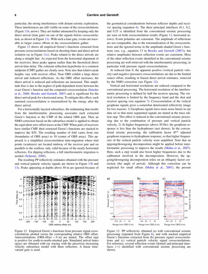
particular, the strong interferences with distant seismic exploration.These interferences are still visible on some of the crosscorrelations(Figure 11b, arrow). They are further attenuated by keeping only thedirect arrival (time gate) on one of the signals before crosscorrela-tion, as shown in Figure 11c. With such a time gate, events are trace-able to larger source offsets in the crosscorrelation gather.Figure 12 shows all empirical Green’s functions extracted from

pressure crosscorrelations based on shooting times and direct arrivalisolation (as in Figure 11c). Peaks related to the direct arrivals arealong a straight line. As expected from the horizontal alignment ofthe receivers, these peaks appear earlier than the theoretical directarrival time delay. The coherent reflection hyperbolas in a commonmidpoint (CMP) gather are clearly seen. Note also that relative peakheights vary with receiver offset. Near OBS exhibit a large directarrival and reduced reflections. As the OBS offset increases, thedirect arrival is reduced and reflections are increased. This ampli-tude bias is due to the neglect of path-dependent terms between theexact Green’s function and the computed crosscorrelation (Sniederet al., 2006; Brooks and Gerstoft, 2007) and is significant for thedirect arrival peak for a horizontal array. To mitigate this effect, eachsummed crosscorrelation is renormalized by the energy after thedirect arrival.For a horizontally-layered subsurface, the redatuming that results

from the interferometric processing associates each extractedGreen’s function to the CMP of the related OBS pair. Then anNMO correction based on the subsurface model is applied to obtainthe equivalent zero-offset traces at the CMP.When pairs of receivershave similar CMP, their extracted Green’s functions are stacked toimprove the S/N. The resulting number of fold varies from one(boundaries of OBS array) to 10 (center of OBS array). This ap-proach is a simplified crosscorrelation time-migration where trialpoints (scatterers) are located midway of the receiver pair and onparallels to the seafloor, only valid because of the nearly horizontalreflectors. For dipping reflectors, a full interferometric migration isneeded (Schuster, 2009).The resulting PP reflectivity estimates obtained with the pressure

and vertical particle velocity signals are shown in Figure 13b and13c. Peaks appearing at depths above 50 m are ignored because of

the geometrical considerations between reflector depths and recei-ver spacing (equation 6). The three principal interfaces (0.1, 0.2,and 0.55 s) identified from the conventional seismic processingare seen on both crosscorrelation results (Figure 13, horizontal ar-rows). Event polarities are consistent. The amplitude of reflectionsare not comparable, due to the renormalization of the crosscorrela-tions and the ignored terms in the amplitude-shaded Green’s func-tions (see, e.g., equation 13 in Brooks and Gerstoft (2007)), butrelative amplitudes between reflection events are consistent. Mostof the other reflection events identified in the conventional seismicprocessing are well retrieved with the interferometric processing, inparticular with pressure signal crosscorrelations.At reduced time 0, the apparent positive (vertical particle velo-

city) and negative (pressure) crosscorrelations are due to the limitedsource offset, resulting in biased direct arrival estimates, removedby the NMO correction (see Figure 12).Vertical and horizontal resolutions are reduced compared to the

conventional processing. The horizontal resolution of the interfero-metric processing is defined by half the receiver spacing. The ver-tical resolution is limited by the frequency band and the shot andreceiver spacing (see equation 7). Crosscorrelation of the verticalgeophone signals gives a somewhat deteriorated reflectivity imagefor two reasons: 1) Geophone signals have more noise bursts in ourdata set so that more segmented signals are muted at the trace edi-tion step. This effect is reduced in the conventional seismic proces-sing due to the combination of pressure and vertical particlevelocity. 2) At higher frequencies (above 50 Hz), the geophone re-sponse is less than the hydrophones (not shown). In the conven-tional seismic processing, the calibration factor Hcal adjustedgeophone response to hydrophone response, so that higher frequen-cies of the vertical particle velocity were amplified. Note that anupgoing/downgoing decomposition might be applied before inter-ferometric processing to improve the results (Mehta et al., 2007).Here, such a step would also boost higher frequencies due to thecalibration involved in the decomposition. However, the up-going/downgoing decomposition relies on an obliquity factor cor-rection (the angle of arrival). Although this correction can beneglected for small offsets (Mehta et al., 2007), the present

!200 !150 !100 !50 0 50 100 150 200

0

0.1

0.2

0.3

0.4

0.5

0.6

OBS relative offset (m)

Tim

e de

lay

(s)

Figure 12. Empirical Green’s functions from pressure signal cross-correlations plotted versus the corresponding relative OBS offset.Autocorrelations (OBSoffset $ 0 m) are muted. The offset signis positive for south-to-north-oriented pair. Simulated arrival times(gray) are obtained with ray tracing with the piecewise increasingvelocity subsurface model with three reflectors. A linear time-variant gain is used.

0

100

200

300

400

500

Dep

th (

m @

1750

m/s

)

0

0.1

0.2

0.3

0.4

0.5

0.6

Range from OBS 6 (m)

Red

uced

TW

T (

s)

Range from OBS 6 (m) Range from OBS 6 (m)

!100 !50 0 50 !100 !50 0 50 !100 !50 0 50

a) b) c)

Figure 13. PP reflectivity obtained (a) with conventional seismicprocessing (repeated from Figure 6), and with stacked empiricalGreen’s functions extracted from (b) pressure signal crosscorrela-tions and (c) vertical particle velocity signal crosscorrelations.For reference, several reflection events (dotted) and principal inter-faces (!) identified with conventional seismic processing areshown.

8 Carrière and Gerstoft

upgoing/downgoing decomposition would not be applicable forpurely ambient noise processing.The seismic interferometry is more sensitive to the velocity mod-

el than the conventional seismic processing. The reason is that thetime migration used in the latter (at the CRG to CDP conversion) isrestricted to small depth-point offsets (up to 100 m, black lines inFigure 5) so that deeper velocities, typically more uncertain, haveless impact on the reflectivity image. In the seismic interferometry,however, the entire velocity model is required for correcting theCMP gathers (Figure 12) on the full image range. This differencewould be less if we were considering only near OBS in the inter-ferometric approach or using larger depth-point offsets in the up-going/downgoing seismic processing.

Implications for ambient noise seismic interferometry

It is not clear that passive seismic interferometry in the frequencyrange of active exploration (10–100 Hz) is realistic, because oceanwaveguide horizontal noise might dominate. That was the case forthe single day of passive data collected here, with a distant seismicexploration dominating the noise distribution from a single direc-tion. This seismic exploration was also present during the activesurveys; see the beamformer output in Figure 2.In terms of processing, passive interferometry is essentially simi-

lar to active interferometry. The interferometric processing schemeused here would be the same if processing passive data, except thatshort-interval crosscorrelation would be based on a sliding overlap-ping time window instead of using the active survey shooting times(see Figure 11). Nevertheless, ambient noise interferometry requiresdifferent preprocessing steps, principally to better respect the as-sumptions required by interferometry theory (source spectrum cor-rection, diffuse noise field, etc.), see, e.g., Bensen et al. (2007);Brooks and Gerstoft (2009b). On the other hand, the problem ofbubble oscillations in active data is absent in ambient noise proces-sing. Passive data might increase the vertical resolution due to adenser source distribution (smaller Δr in equation 7). Active dataprocessing benefits from the isolation of direct arrival (see Fig-ure 11c) which efficiently attenuates spurious arrivals.Ambient noise survey requires long-term monitoring for redu-

cing signals that bias the noise distribution. Here, the presenceof another survey from a fixed location is an example where a long-er term deployment would have been useful. As an alternative,using many sensors on a 2D or 3D grid would enable array proces-sing techniques to filter unwanted signals.

CONCLUSION

The Green’s function extraction from active OBS data iscompared to conventional seismic processing based on upgoing/downgoing decomposition and deconvolution. Assuming a simplesubsurface velocity model, both methods successfully localize thestrong reflectors previously identified from oil-industry data. Theinterferometric processing reduces the horizontal resolution to halfthe sensor spacing whereas the standard seismic processing hori-zontal resolution is limited by the shot spacing. A higher resolutionis obtained with the crosscorrelation of the pressure signals, the ver-tical particle velocity signals being characterized here by a lowerfrequency content.Compared to the upgoing/downgoing decomposition scheme, the

Green’s function extraction does not require knowledge of source

position. The short-interval crosscorrelation time windows can bedefined independently from the shooting times. However, usingthe shooting times optimally frames the crosscorrelations andwas found to reduce interferences from other acoustic sources. In-terferences were further attenuated by isolating the direct arrival onone of the signals before crosscorrelation.Active source signals are usually characterized by bubble pulses

that affect the crosscorrelations. Here, the strong bubble pulse isefficiently removed by deconvolving the traces with the wavelet es-timated from the upgoing/downgoing processing.

ACKNOWLEDGMENTS

The authors acknowledge Marco D’Emidio, University ofMississippi, for providing Figure 1a. Seismic data on Figure 4 wereprovided by WesternGeco. This work was supported by DOENTEL, DOI BOEM, and DOC NOAA NIUST, via the Gulf ofMexico Hydrates Research Consortium, and by the NSF (EAR-0944109 and OCE-1030022).

REFERENCES

Amundsen, L., 2001, Elimination of free-surface related multiples withoutneed of the source wavelet: Geophysics, 66, 327–341, doi: 10.1190/1.1444912.

Amundsen, L., and A. Reitan, 1995, Decomposition of multicomponent sea-floor data into upgoing and downgoing P- and S-waves: Geophysics, 60,563–572, doi: 10.1190/1.1443794.

Backus, M. M., P. E. Murray, and R. J. Graebner, 2007, OBC sensorresponse and calibrated reflectivity: 77th Annual International Meeting,SEG, Expanded Abstracts, 1044–1048.

Backus, M. M., P. E. Murray, B. A. Hardage, and R. J. Graebner, 2006,High-resolution multicomponent seismic imaging of deepwater gas-hy-drate systems: The Leading Edge, 25, 578–596, doi: 10.1190/1.2202662.

Bakulin, A., and R. Calvert, 2006, The virtual source method: Theory andcase study: Geophysics, 71, no. 4, SI139–SI150, doi: 10.1190/1.2216190.

Bensen, G. D., M. H. Ritzwoller, M. P. Barmin, A. L. Levshin, F. Lin, M. P.Moschetti, N. M. Shapiro, and Y. Yang, 2007, Processing seismic ambientnoise data to obtain reliable broad-band surface wave dispersion measure-ments: Geophysical Journal International, 169, 1239–1260, doi: 10.1111/gji.2007.169.issue-3.

Bharadwaj, P., G. T. Schuster, I. Mallinson, and W. Dai, 2012, Theory ofsupervirtual refraction interferometry: Geophysical Journal International,188, 263–273, doi: 10.1111/gji.2012.188.issue-1.

Bowen, A. N., 1986, A comparison of statistical and deterministic Wienerdeconvolution of deep-tow seismic data: Geophysical Prospecting, 34,366–382, doi: 10.1111/gpr.1986.34.issue-3.

Brooks, L. A., and P. Gerstoft, 2007, Ocean acoustic interferometry: Journalof the Acoustical Society of America, 121, 3377–3385, doi: 10.1121/1.2723650.

Brooks, L. A., and P. Gerstoft, 2009a, Green’s function approximation fromcross-correlation of active sources in the ocean: Journal of the AcousticalSociety of America, 126, 46–55, doi: 10.1121/1.3143143.

Brooks, L. A., and P. Gerstoft, 2009b, Green’s function approximation fromcross-correlations of 20–100 Hz noise during a tropical storm: Journal ofthe Acoustical Society of America, 125, 723–34, doi: 10.1121/1.3056563.

Dash, R., G. Spence, R. Hyndman, S. Grion, Y. Wang, and S. Ronen, 2009,Wide-area imaging from OBS multiples: Geophysics, 74, no. 6, Q41–Q47, doi: 10.1190/1.3223623.

de Ridder, S., and J. Dellinger, 2011, Ambient seismic noise eikonal tomo-graphy for near-surface imaging at Valhall: The Leading Edge, 30, 506–512, doi: 10.1190/1.3589108.

Dong, S., J. Sheng, and G. T. Schuster, 2006, Theory and practice of refrac-tion interferometry: 76th Annual International Meeting, SEG, ExpandedAbstracts, 3021–3025.

Draganov, D., K. Wapenaar, W. Mulder, J. Singer, and A. Verdel, 2007,Retrieval of reflections from seismic background-noise measurements:Geophysical Research Letters, 34, L04305, doi: 10.1029/2006GL028735.

Gaiser, J., and I. Vasconcelos, 2010, Elastic interferometry for ocean bottomcable data: Theory and examples: Geophysical Prospecting, 58, 347–360,doi: 10.1111/(ISSN)1365-2478.

Gerstoft, P., K. G. Sabra, P. Roux, W. A. Kuperman, and M. C. Fehler, 2006,Green’s functions extraction and surface-wave tomography from micro-seisms in southern California: Geophysics, 71, no. 4, SI23–SI31, doi: 10.1190/1.2210607.

1

Subsurface imaging using OBS interferometry 9

Haines, S. S., 2011, PP and PS interferometric images of near-seafloor sedi-ments: 81st Annual International Meeting, SEG, Expanded Abstracts,1288–1292.

Harmon, N., D. Forsyth, and S. Webb, 2007, Using ambient seismic noise todetermine short-period phase velocities and shallow shear velocities inyoung oceanic lithosphere: Bulletin of the Seismological Society ofAmerica, 97, 2009–2023, doi: 10.1785/0120070050.

Hatchell, P., and K. Mehta, 2010, Ocean-bottom seismic (OBS) timing driftcorrection using passive seismic data: 80th Annual International Meeting,SEG, Expanded Abstracts, 2054–2058.

Hohl, D., and A. Mateeva, 2006, Passive seismic reflectivity imagingwith ocean-bottom cable data: 76th Annual International Meeting,SEG, Expanded Abstracts, 1560–1564.

Jiang, Z., J. Yu, G. T. Schuster, and B. E. Hornby, 2005, Migration of multi-ples: The Leading Edge, 24, 315–318, doi: 10.1190/1.1895318.

Li, J., S. Jin, and S. Ronen, 2004, Data-driven tilt angle estimation of multi-component receivers: 74th Annual International Meeting, SEG, ExpandedAbstracts, 23, 921–924.

Loewenthal, D., S. S. Lee, and G. H. F. Gardner, 1985, Deterministic esti-mation of a wavelet using impedance type technique: GeophysicalProspecting, 33, 956–969, doi: 10.1111/gpr.1985.33.issue-7.

Macelloni, L., A. Simonetti, J. H. Knapp, C. C. Knapp, C. B. Lutken, and L.L. Lapham, 2012, Multiple resolution seismic imaging of a shallow hy-drocarbon plumbing system, Woolsey Mound, Northern Gulf of Mexico:Marine and Petroleum Geology, 38, 128–142, doi: 10.1016/j.marpetgeo.2012.06.010.

McGee, T., J. Woolsey, C. Lutken, L. Macelloni, L. Lapham, B. Battista, S.Caruso, and V. Goebel, 2009, A multidisciplinary sea-floor observatory inthe Northern Gulf of Mexico: Results of preliminary studies: OCEANS2009, MTS/IEEE Biloxi-Marine Technology for Our Future: Global andLocal Challenges, 1–5.

Mehta, K., A. Bakulin, J. Sheiman, R. Calvert, and R. Snieder, 2007,Improving the virtual source method by wavefield separation: Geo-physics, 72, no. 4, V79–V86, doi: 10.1190/1.2733020.

Minato, S., T. Matsuoka, T. Tsuji, D. Draganov, J. Hunziker, and K.Wapenaar, 2011, Seismic interferometry using multidimensional decon-volution and crosscorrelation for crosswell seismic reflection data withoutborehole sources: Geophysics, 76, no. 1, SA19–SA34, doi: 10.1190/1.3511357.

Minato, S., T. Tsuji, T. Matsuoka, and K. Obana, 2012, Crosscorrelation ofearthquake data using stationary phase evaluation: insight into reflectionstructures of oceanic crust surface in the Nankai Trough: InternationalJournal of Geophysics, 2012, 1–8, doi: 10.1155/2012/101545.

Miyazawa, M., R. Snieder, and A. Venkataraman, 2008, Application of seis-mic interferometry to extract P- and S-wave propagation and observationof shear-wave splitting from noise data at Cold Lake, Alberta, Canada:Geophysics, 73, no. 4, D35–D40, doi: 10.1190/1.2937172.

Murray, P., and M. DeAngelo, 2008, Simultaneous P-and S-wave intervalvelocity model building of near-seafloor geology using OBC data: 78thAnnual International Meeting, SEG, Expanded Abstracts, 1038–1042.

Rickett, J., and J. Claerbout, 1999, Acoustic daylight imaging via spectralfactorization: Helioseismology and reservoir monitoring: The LeadingEdge, 18, 957–960, doi: 10.1190/1.1438420.

Roux, P., K. G. Sabra, P. Gerstoft, W. A. Kuperman, and M. C. Fehler, 2005,P-waves from cross-correlation of seismic noise: Geophysical ResearchLetters, 32, L19303, doi: 10.1029/2005GL023803.

Sabra, K. G., P. Roux, and W. A. Kuperman, 2005, Arrival-time structure ofthe time-averaged ambient noise cross-correlation function in an oceanicwaveguide: Journal of the Acoustical Society of America, 117, 164–174,doi: 10.1121/1.1835507.

Schalkwijk, K. M., C. P. A. Wapenaar, and D. J. Verschuur, 1999, Applica-tion of two-step decomposition to multicomponent ocean-bottom data:Theory and case study: Journal of Seismic Exploration, 8, 261–278.

Schneider, W. A., and M. M. Backus, 1964, Ocean-bottom seismic measure-ments off the California coast: Journal of Geophysical Research, 69,1135–1143, doi: 10.1029/JZ069i006p01135.

Schuster, G. T., 2009, Seismic interferometry: Cambridge University Press.Schuster, G. T., J. Yu, J. Sheng, and J. Rickett, 2004, Interferometric/

daylight seismic imaging: Geophysical Journal International, 157,838–852, doi: 10.1111/gji.2004.157.issue-2.

Schuster, G. T., and M. Zhou, 2006, A theoretical overview of model-basedand correlation-based redatuming methods: Geophysics, 71, no. 4, SI103–SI110, doi: 10.1190/1.2208967.

Shapiro, N. M., and M. Campillo, 2004, Emergence of broadband Rayleighwaves from correlations of the ambient seismic noise: GeophysicalResearch Letters, 31, L07614, doi: 10.1029/2004GL019491.

Shapiro, N. M., M. Campillo, L. Stehly, and M. H. Ritzwoller, 2005, High-resolution surface-wave tomography from ambient seismic noise:Science, 307, 1615–1618, doi: 10.1126/science.1108339.

Sheley, D., and G. T. Schuster, 2003, Reduced time migration oftransmission PS waves: Geophysics, 68, 1695–1707, doi: 10.1190/1.1620643.

Snieder, R., A. Grêt, H. Douma, and J. Scales, 2002, Coda wave inter-ferometry for estimating nonlinear behavior in seismic velocity: Science,295, 2253–2255, doi: 10.1126/science.1070015.

Snieder, R., K. Wapenaar, and K. Larner, 2006, Spurious multiples in seis-mic interferometry of primaries: Geophysics, 71, no. 4, SI111–SI124, doi:10.1190/1.2211507.

Van Veen, B. D., and K. M. Buckley, 1988, Beamforming: A versatileapproach to spatial filtering: IEEE Transactions on Acoustics, Speech,and Signal Processing, 5, 4–24.

Vasconcelos, I., R. Snieder, and B. Hornby, 2008, Imaging internal multiplesfrom subsalt VSP data — Examples of target-oriented interferometry:Geophysics, 73, no. 4, S157–S168, doi: 10.1190/1.2944168.

Wapenaar, K., 2004, Retrieving the elastodynamic Green’s function of anarbitrary inhomogeneous medium by cross correlation: Physical ReviewLetters, 93, 254301, doi: 10.1103/PhysRevLett.93.254301.

Wapenaar, K., 2006, Green’s function retrieval by cross-correlation in caseof one-sided illumination: Geophysical Research Letters, 33, L19304,doi: 10.1029/2006GL027747.

Wapenaar, K., D. Draganov, and J. O. A. Robertsson, 2006, Seismic inter-ferometry: History and present status: Geophysics, 71, no. 4, SI1–SI4,doi: 10.1190/gpysa7.71.si1_1.

Wapenaar, K., D. Draganov, R. Snieder, X. Campman, and A. Verdel, 2010a,Tutorial on seismic interferometry: Part 1 — Basic principles andapplications: Geophysics, 75, no. 5, 75A195–75A209, doi: 10.1190/1.3457445.

Wapenaar, K., D. Draganov, and J. Thorbecke, 2002, Theory of acousticdaylight imaging revisited: 72nd Annual International Meeting, SEG,Expanded Abstracts, 2269–2272.

Wapenaar, K., E. Slob, R. Snieder, and A. Curtis, 2010b, Tutorial on seismicinterferometry: Part 2 — Underlying theory and new advances: Geophy-sics, 75, no. 5, 75A211–75A227, doi: 10.1190/1.3463440.

Wood, W. T., P. E. Hart, D. R. Hutchinson, N. Dutta, F. Snyder, R. B. Coffin,and J. F. Gettrust, 2008, Gas and gas hydrate distribution around seafloorseeps in Mississippi Canyon, Northern Gulf of Mexico, using multi-resolution seismic imagery: Marine and Petroleum Geology, 25, 952–959, doi: 10.1016/j.marpetgeo.2008.01.015.

Yao, H., P. Gouédard, J. A. Collins, J. J. McGuire, and R. D. van der Hilst,2011, Structure of young East Pacific Rise lithosphere from ambient noisecorrelation analysis of fundamental- and higher-mode Scholte-Rayleighwaves: Comptes Rendus Geoscience, 343, 571–583, doi: 10.1016/j.crte.2011.04.004.

Yu, J., and G. T. Schuster, 2006, Crosscorrelogram migration of inversevertical seismic profile data: Geophysics, 71, no. 1, S1–S11, doi: 10.1190/1.2159056.

2

3

10 Carrière and Gerstoft

Queries

1. A check of online databases revealed a possible error in this reference. (Gaiser et al., 2010) The year has been changed from'2009' to '2010'. Please confirm this is correct.

2. A check of online databases revealed a possible error in this reference. (Minato et al., 2012) The page number has beenchanged from '101545' to '1-8'. Please confirm this is correct.

3. This query was generated by an automatic reference checking system. This reference (Schalkwijk et al., 1999) could not belocated in the databases used by the system. While the reference may be correct, we ask that you check it so we can provideas many links to the referenced articles as possible.

Subsurface imaging using OBS interferometry 11