Deep Sentence Embedding Using Long Short-Term Memory ... · 1 Deep Sentence Embedding Using Long...

1

Deep Sentence Embedding Using LongShort-Term Memory Networks: Analysis and

Application to Information RetrievalHamid Palangi, Li Deng, Yelong Shen, Jianfeng Gao, Xiaodong He, Jianshu Chen, Xinying Song,

Rabab Ward

Abstract—This paper develops a model that addressessentence embedding, a hot topic in current natural lan-guage processing research, using recurrent neural networks(RNN) with Long Short-Term Memory (LSTM) cells. Theproposed LSTM-RNN model sequentially takes each wordin a sentence, extracts its information, and embeds it intoa semantic vector. Due to its ability to capture long termmemory, the LSTM-RNN accumulates increasingly richerinformation as it goes through the sentence, and when itreaches the last word, the hidden layer of the networkprovides a semantic representation of the whole sentence.In this paper, the LSTM-RNN is trained in a weaklysupervised manner on user click-through data logged by acommercial web search engine. Visualization and analysisare performed to understand how the embedding processworks. The model is found to automatically attenuate theunimportant words and detects the salient keywords inthe sentence. Furthermore, these detected keywords arefound to automatically activate different cells of the LSTM-RNN, where words belonging to a similar topic activate thesame cell. As a semantic representation of the sentence,the embedding vector can be used in many differentapplications. These automatic keyword detection and topicallocation abilities enabled by the LSTM-RNN allow thenetwork to perform document retrieval, a difficult languageprocessing task, where the similarity between the query anddocuments can be measured by the distance between theircorresponding sentence embedding vectors computed bythe LSTM-RNN. On a web search task, the LSTM-RNNembedding is shown to significantly outperform severalexisting state of the art methods. We emphasize that theproposed model generates sentence embedding vectors thatare specially useful for web document retrieval tasks. Acomparison with a well known general sentence embeddingmethod, the Paragraph Vector, is performed. The resultsshow that the proposed method in this paper significantlyoutperforms it for web document retrieval task.

Index Terms—Deep Learning, Long Short-Term Mem-ory, Sentence Embedding.

I. INTRODUCTION

H. Palangi and R. Ward are with the Department of Electrical andComputer Engineering, University of British Columbia, Vancouver,BC, V6T 1Z4 Canada (e-mail: {hamidp,rababw}@ece.ubc.ca)

L. Deng, Y. Shen, J.Gao, X. He, J. Chen and X. Song arewith Microsoft Research, Redmond, WA 98052 USA (e-mail:{deng,jfgao,xiaohe,yeshen,jianshuc,xinson}@microsoft.com)

LEARNING a good representation (or features) ofinput data is an important task in machine learning.

In text and language processing, one such problem islearning of an embedding vector for a sentence; that is, totrain a model that can automatically transform a sentenceto a vector that encodes the semantic meaning of thesentence. While word embedding is learned using aloss function defined on word pairs, sentence embeddingis learned using a loss function defined on sentencepairs. In the sentence embedding usually the relationshipamong words in the sentence, i.e., the context informa-tion, is taken into consideration. Therefore, sentence em-bedding is more suitable for tasks that require computingsemantic similarities between text strings. By mappingtexts into a unified semantic representation, the embed-ding vector can be further used for different languageprocessing applications, such as machine translation [1],sentiment analysis [2], and information retrieval [3].In machine translation, the recurrent neural networks(RNN) with Long Short-Term Memory (LSTM) cells, orthe LSTM-RNN, is used to encode an English sentenceinto a vector, which contains the semantic meaning ofthe input sentence, and then another LSTM-RNN isused to generate a French (or another target language)sentence from the vector. The model is trained to bestpredict the output sentence. In [2], a paragraph vectoris learned in an unsupervised manner as a distributedrepresentation of sentences and documents, which arethen used for sentiment analysis. Sentence embeddingcan also be applied to information retrieval, where thecontextual information are properly represented by thevectors in the same space for fuzzy text matching [3].

In this paper, we propose to use an RNN to sequen-tially accept each word in a sentence and recurrently mapit into a latent space together with the historical informa-tion. As the RNN reaches the last word in the sentence,the hidden activations form a natural embedding vectorfor the contextual information of the sentence. We furtherincorporate the LSTM cells into the RNN model (i.e. theLSTM-RNN) to address the difficulty of learning longterm memory in RNN. The learning of such a model

arX

iv:1

502.

0692

2v3

[cs

.CL

] 1

6 Ja

n 20

16

2

is performed in a weakly supervised manner on theclick-through data logged by a commercial web searchengine. Although manually labelled data are insufficientin machine learning, logged data with limited feedbacksignals are massively available due to the widely usedcommercial web search engines. Limited feedback in-formation such as click-through data provides a weaksupervision signal that indicates the semantic similaritybetween the text on the query side and the clicked texton the document side. To exploit such a signal, theobjective of our training is to maximize the similaritybetween the two vectors mapped by the LSTM-RNNfrom the query and the clicked document, respectively.Consequently, the learned embedding vectors of thequery and clicked document are specifically useful forweb document retrieval task.

An important contribution of this paper is to analysethe embedding process of the LSTM-RNN by visualizingthe internal activation behaviours in response to differenttext inputs. We show that the embedding process of thelearned LSTM-RNN effectively detects the keywords,while attenuating less important words, in the sentenceautomatically by switching on and off the gates withinthe LSTM-RNN cells. We further show that differentcells in the learned model indeed correspond to differ-ent topics, and the keywords associated with a similartopic activate the same cell unit in the model. As theLSTM-RNN reads to the end of the sentence, the topicactivation accumulates and the hidden vector at the lastword encodes the rich contextual information of theentire sentence. For this reason, a natural applicationof sentence embedding is web search ranking, in whichthe embedding vector from the query can be used tomatch the embedding vectors of the candidate documentsaccording to the maximum cosine similarity rule. Evalu-ated on a real web document ranking task, our proposedmethod significantly outperforms many of the existingstate of the art methods in NDCG scores. Please notethat when we refer to document in the paper we meanthe title (headline) of the document.

II. RELATED WORK

Inspired by the word embedding method [4], [5], theauthors in [2] proposed an unsupervised learning methodto learn a paragraph vector as a distributed representationof sentences and documents, which are then used forsentiment analysis with superior performance. However,the model is not designed to capture the fine-grainedsentence structure. In [6], an unsupervised sentenceembedding method is proposed with great performanceon large corpus of contiguous text corpus, e.g., theBookCorpus [7]. The main idea is to encode the sentences(t) and then decode previous and next sentences, i.e.,

s(t−1) and s(t+1), using two separate decoders. The en-coder and decoders are RNNs with Gated Recurrent Unit(GRU) [8]. However, this sentence embedding methodis not designed for document retrieval task having asupervision among queries and clicked and unclickeddocuments. In [9], a Semi-Supervised Recursive Au-toencoder (RAE) is proposed and used for sentimentprediction. Similar to our proposed method, it does notneed any language specific sentiment parsers. A greedyapproximation method is proposed to construct a treestructure for the input sentence. It assigns a vector perword. It can become practically problematic for largevocabularies. It also works both on unlabeled data andsupervised sentiment data.

Similar to the recurrent models in this paper, TheDSSM [3] and CLSM [10] models, developed for in-formation retrieval, can also be interpreted as sentenceembedding methods. However, DSSM treats the inputsentence as a bag-of-words and does not model worddependencies explicitly. CLSM treats a sentence as a bagof n-grams, where n is defined by a window, and cancapture local word dependencies. Then a Max-poolinglayer is used to form a global feature vector. Methods in[11] are also convolutional based networks for NaturalLanguage Processing (NLP). These models, by design,cannot capture long distance dependencies, i.e., depen-dencies among words belonging to non-overlapping n-grams. In [12] a Dynamic Convolutional Neural Network(DCNN) is proposed for sentence embedding. Similar toCLSM, DCNN does not rely on a parse tree and is easilyapplicable to any language. However, different fromCLSM where a regular max-pooling is used, in DCNN adynamic k-max-pooling is used. This means that insteadof just keeping the largest entries among word vectors inone vector, k largest entries are kept in k different vec-tors. DCNN has shown good performance in sentimentprediction and question type classification tasks. In [13],a convolutional neural network architecture is proposedfor sentence matching. It has shown great performance inseveral matching tasks. In [14], a Bilingually-constrainedRecursive Auto-encoders (BRAE) is proposed to createsemantic vector representation for phrases. Through ex-periments it is shown that the proposed method has greatperformance in two end-to-end SMT tasks.

Long short-term memory networks were developedin [15] to address the difficulty of capturing long termmemory in RNN. It has been successfully applied tospeech recognition, which achieves state-of-art perfor-mance [16], [17]. In text analysis, LSTM-RNN treats asentence as a sequence of words with internal structures,i.e., word dependencies. It encodes a semantic vector ofa sentence incrementally which differs from DSSM andCLSM. The encoding process is performed left-to-right,word-by-word. At each time step, a new word is encoded

3

into the semantic vector, and the word dependenciesembedded in the vector are “updated”. When the processreaches the end of the sentence, the semantic vector hasembedded all the words and their dependencies, hence,can be viewed as a feature vector representation of thewhole sentence. In the machine translation work [1], aninput English sentence is converted into a vector repre-sentation using LSTM-RNN, and then another LSTM-RNN is used to generate an output French sentence.The model is trained to maximize the probability ofpredicting the correct output sentence. In [18], there aretwo main composition models, ADD model that is bagof words and BI model that is a summation over bi-grampairs plus a non-linearity. In our proposed model, insteadof simple summation, we have used LSTM model withletter tri-grams which keeps valuable information overlong intervals (for long sentences) and throws away use-less information. In [19], an encoder-decoder approach isproposed to jointly learn to align and translate sentencesfrom English to French using RNNs. The concept of“attention” in the decoder, discussed in this paper, isclosely related to how our proposed model extractskeywords in the document side. For further explanationsplease see section V-A2. In [20] a set of visualizationsare presented for RNNs with and without LSTM cellsand GRUs. Different from our work where the target taskis sentence embedding for document retrieval, the targettasks in [20] were character level sequence modelling fortext characters and source codes. Interesting observationsabout interpretability of some LSTM cells and statisticsof gates activations are presented. In section V-A weshow that some of the results of our visualization areconsistent with the observations reported in [20]. Wealso present more detailed visualization specific to thedocument retrieval task using click-through data. We alsopresent visualizations about how our proposed model canbe used for keyword detection.

Different from the aforementioned studies, the methoddeveloped in this paper trains the model so that sentencesthat are paraphrase of each other are close in theirsemantic embedding vectors — see the description inSec. IV further ahead. Another reason that LSTM-RNNis particularly effective for sentence embedding, is itsrobustness to noise. For example, in the web documentranking task, the noise comes from two sources: (i) Notevery word in query / document is equally important,and we only want to “remember” salient words usingthe limited “memory”. (ii) A word or phrase that isimportant to a document may not be relevant to agiven query, and we only want to “remember” relatedwords that are useful to compute the relevance of thedocument for a given query. We will illustrate robustnessof LSTM-RNN in this paper. The structure of LSTM-RNN will also circumvent the serious limitation of using

a fixed window size in CLSM. Our experiments showthat this difference leads to significantly better results inweb document retrieval task. Furthermore, it has otheradvantages. It allows us to capture keywords and keytopics effectively. The models in this paper also do notneed the extra max-pooling layer, as required by theCLSM, to capture global contextual information and theydo so more effectively.

III. SENTENCE EMBEDDING USING RNNS WITH ANDWITHOUT LSTM CELLS

In this section, we introduce the model of recurrentneural networks and its long short-term memory versionfor learning the sentence embedding vectors. We startwith the basic RNN and then proceed to LSTM-RNN.

A. The basic version of RNN

The RNN is a type of deep neural networks thatare “deep” in temporal dimension and it has been usedextensively in time sequence modelling [21], [22], [23],[24], [25], [26], [27], [28], [29]. The main idea of usingRNN for sentence embedding is to find a dense andlow dimensional semantic representation by sequentiallyand recurrently processing each word in a sentence andmapping it into a low dimensional vector. In this model,the global contextual features of the whole text will bein the semantic representation of the last word in thetext sequence — see Figure 1, where x(t) is the t-thword, coded as a 1-hot vector, Wh is a fixed hashingoperator similar to the one used in [3] that converts theword vector to a letter tri-gram vector, W is the inputweight matrix, Wrec is the recurrent weight matrix, y(t)is the hidden activation vector of the RNN, which can beused as a semantic representation of the t-th word, andy(t) associated to the last word x(m) is the semanticrepresentation vector of the entire sentence. Note thatthis is very different from the approach in [3] where thebag-of-words representation is used for the whole textand no context information is used. This is also differentfrom [10] where the sliding window of a fixed size (akinto an FIR filter) is used to capture local features and amax-pooling layer on the top to capture global features.In the RNN there is neither a fixed-sized window nora max-pooling layer; rather the recurrence is used tocapture the context information in the sequence (akinto an IIR filter).

The mathematical formulation of the above RNNmodel for sentence embedding can be expressed as

l(t) = Whx(t)

y(t) = f(Wl(t) + Wrecy(t− 1) + b) (1)

where W and Wrec are the input and recurrent matricesto be learned, Wh is a fixed word hashing operator, b

4

…

Embedding vector

𝒍(2) 𝒍(1) 𝒍(𝑚)

Fig. 1. The basic architecture of the RNN for sentence embedding,where temporal recurrence is used to model the contextual informationacross words in the text string. The hidden activation vector corre-sponding to the last word is the sentence embedding vector (blue).

is the bias vector and f(·) is assumed to be tanh(·).Note that the architecture proposed here for sentenceembedding is slightly different from traditional RNN inthat there is a word hashing layer that convert the highdimensional input into a relatively lower dimensionalletter tri-gram representation. There is also no per wordsupervision during training, instead, the whole sentencehas a label. This is explained in more detail in sectionIV.

B. The RNN with LSTM cells

Although RNN performs the transformation from thesentence to a vector in a principled manner, it is generallydifficult to learn the long term dependency within thesequence due to vanishing gradients problem. One ofthe effective solutions for this problem in RNNs isusing memory cells instead of neurons originally pro-posed in [15] as Long Short-Term Memory (LSTM) andcompleted in [30] and [31] by adding forget gate andpeephole connections to the architecture.

We use the architecture of LSTM illustrated in Fig.2 for the proposed sentence embedding method. In thisfigure, i(t), f(t) ,o(t) , c(t) are input gate, forget gate,output gate and cell state vector respectively, Wp1, Wp2

and Wp3 are peephole connections, Wi, Wreci and bi,i = 1, 2, 3, 4 are input connections, recurrent connectionsand bias values, respectively, g(·) and h(·) are tanh(·)function and σ(·) is the sigmoid function. We use thisarchitecture to find y for each word, then use the y(m)corresponding to the last word in the sentence as thesemantic vector for the entire sentence.

Considering Fig. 2, the forward pass for LSTM-RNN

𝒙(𝑡)

𝑾ℎ

𝒍(𝑡)

𝑾3

𝒙(𝑡)

𝑾ℎ

𝒍(𝑡)

𝑾4

𝒙(𝑡)

𝑾ℎ

𝒍(𝑡)

𝑾2

𝒙(𝑡)

𝑾ℎ

𝒍(𝑡)

𝑾1

𝑔(. )

𝜎(. ) 𝜎(. ) Input Gate Output Gate

𝜎(. ) Forget Gate

Cell ×

𝒚𝑔(𝑡)

𝒊(𝑡)

𝒇(𝑡)

𝒄(𝑡 − 1) ×

ℎ(. )

×

𝒄(𝑡)

𝒐(𝑡)

𝒚(𝑡)

𝒄(𝑡 − 1)

𝑾𝑝2

𝑾𝑝3 𝑾𝑝1

𝒚(𝑡 − 1)

𝑾𝑟𝑒𝑐4

𝟏

𝒃4

𝒚(𝑡 − 1)

𝟏

𝑾𝑟𝑒𝑐3 𝒃3

𝟏

𝒃1

𝑾𝑟𝑒𝑐1

𝒚(𝑡 − 1)

𝟏

𝒃2

𝒚(𝑡 − 1)

𝑾𝑟𝑒𝑐2

Fig. 2. The basic LSTM architecture used for sentence embedding

model is as follows:

yg(t) = g(W4l(t) + Wrec4y(t− 1) + b4)

i(t) = σ(W3l(t) + Wrec3y(t− 1) + Wp3c(t− 1) + b3)

f(t) = σ(W2l(t) + Wrec2y(t− 1) + Wp2c(t− 1) + b2)

c(t) = f(t) ◦ c(t− 1) + i(t) ◦ yg(t)

o(t) = σ(W1l(t) + Wrec1y(t− 1) + Wp1c(t) + b1)

y(t) = o(t) ◦ h(c(t)) (2)

where ◦ denotes Hadamard (element-wise) product. Adiagram of the proposed model with more details ispresented in section VI of Supplementary Materials.

IV. LEARNING METHOD

To learn a good semantic representation of the inputsentence, our objective is to make the embedding vectorsfor sentences of similar meaning as close as possible,and meanwhile, to make sentences of different meaningsas far apart as possible. This is challenging in practicesince it is hard to collect a large amount of manuallylabelled data that give the semantic similarity signalbetween different sentences. Nevertheless, the widelyused commercial web search engine is able to logmassive amount of data with some limited user feedbacksignals. For example, given a particular query, the click-through information about the user-clicked documentamong many candidates is usually recorded and can beused as a weak (binary) supervision signal to indicatethe semantic similarity between two sentences (on thequery side and the document side). In this section, weexplain how to leverage such a weak supervision signalto learn a sentence embedding vector that achieves theaforementioned training objective. Please also note thatabove objective to make sentences with similar meaningas close as possible is similar to machine translation

5

yQ(TQ)

yD+(TD+)

yD�1(TD�

1)

yD�n(TD�

n)

Click:'1'

…'

0'

0'

Nega/ve'samples'

Posi/ve'sample'

Fig. 3. The click-through signal can be used as a (binary) indicationof the semantic similarity between the sentence on the query side andthe sentence on the document side. The negative samples are randomlysampled from the training data.

tasks where two sentences belong to two different lan-guages with similar meanings and we want to make theirsemantic representation as close as possible.

We now describe how to train the model to achieve theabove objective using the click-through data logged by acommercial search engine. For a complete description ofthe click-through data please refer to section 2 in [32].To begin with, we adopt the cosine similarity betweenthe semantic vectors of two sentences as a measure fortheir similarity:

R(Q,D) =yQ(TQ)TyD(TD)

‖yQ(TQ)‖ · ‖yD(TD)‖(3)

where TQ and TD are the lengths of the sentenceQ and sentence D, respectively. In the context oftraining over click-through data, we will use Q andD to denote “query” and “document”, respectively.In Figure 3, we show the sentence embedding vec-tors corresponding to the query, yQ(TQ), and all thedocuments, {yD+(TD+),yD−1

(TD−1), . . . ,yD−n (TD−n )},

where the subscript D+ denotes the (clicked) positivesample among the documents, and the subscript D−jdenotes the j-th (un-clicked) negative sample. All theseembedding vectors are generated by feeding the sen-tences into the RNN or LSTM-RNN model describedin Sec. III and take the y corresponding to the last word— see the blue box in Figure 1.

We want to maximize the likelihood of the clickeddocument given query, which can be formulated as thefollowing optimization problem:

L(Λ) = minΛ

{− log

N∏r=1

P (D+r |Qr)

}= min

Λ

N∑r=1

lr(Λ)

(4)where Λ denotes the collection of the model parameters;in regular RNN case, it includes Wrec and W in Figure1, and in LSTM-RNN case, it includes W1, W2, W3,W4, Wrec1, Wrec2, Wrec3, Wrec4, Wp1, Wp2, Wp3,b1, b2, b3 and b4 in Figure 2. D+

r is the clickeddocument for r-th query, P (D+

r |Qr) is the probability

of clicked document given the r-th query, N is numberof query / clicked-document pairs in the corpus and

lr(Λ) = − log

eγR(Qr,D+r )

eγR(Qr,D+r ) +

∑ni=j e

γR(Qr,D−r,j)

= log

1 +

n∑j=1

e−γ·∆r,j

(5)

where ∆r,j = R(Qr, D+r ) − R(Qr, D

−r,j), R(·, ·) was

defined earlier in (3), D−r,j is the j-th negative candidatedocument for r-th query and n denotes the number ofnegative samples used during training.

The expression in (5) is a logistic loss over ∆r,j .It upper-bounds the pairwise accuracy, i.e., the 0 - 1loss. Since the similarity measure is the cosine function,∆r,j ∈ [−2, 2]. To have a larger range for ∆r,j , we useγ for scaling. It helps to penalize the prediction errormore. Its value is set empirically by experiments on aheld out dataset.

To train the RNN and LSTM-RNN, we use Back Prop-agation Through Time (BPTT). The update equations forparameter Λ at epoch k are as follows:

4Λk = Λk −Λk−1

4Λk = µk−14Λk−1 − εk−1∇L(Λk−1 + µk−14Λk−1)(6)

where ∇L(·) is the gradient of the cost function in (4),ε is the learning rate and µk is a momentum parameterdetermined by the scheduling scheme used for training.Above equations are equivalent to Nesterov methodin [33]. To see why, please refer to appendix A.1 of[34] where Nesterov method is derived as a momentummethod. The gradient of the cost function, ∇L(Λ), is:

∇L(Λ) = −N∑r=1

n∑j=1

T∑τ=0

αr,j∂∆r,j,τ

∂Λ︸︷︷︸one large update

(7)

where T is the number of time steps that we unfold thenetwork over time and

αr,j =−γe−γ∆r,j

1 +∑nj=1 e

−γ∆r,j. (8)

∂∆r,j,τ

∂Λ in (7) and error signals for different param-eters of RNN and LSTM-RNN that are necessary fortraining are presented in Appendix A. Full derivation ofgradients in both models is presented in section III ofsupplementary materials.

To accelerate training by parallelization, we use mini-batch training and one large update instead of incremen-tal updates during back propagation through time. Toresolve the gradient explosion problem we use gradient

6

Algorithm 1 Training LSTM-RNN for Sentence Embed-ding

Inputs: Fixed step size “ε”, Scheduling for “µ”, Gradient clip threshold“thG”, Maximum number of Epochs “nEpoch”, Total number of query/ clicked-document pairs “N”, Total number of un-clicked (negative) docu-ments for a given query “n”, Maximum sequence length for truncated BPTT“T ”.Outputs: Two trained models, one in query side “ΛQ”, one in documentside “ΛD”.Initialization: Set all parameters in ΛQ and ΛD to small random numbers,i = 0, k = 1.procedure LSTM-RNN(ΛQ,ΛD)

while i ≤ nEpoch dofor “first minibatch” → “last minibatch” dor ← 1while r ≤ N do

for j = 1→ n doCompute αr,j . use (8)Compute

∑Tτ=0 αr,j

∂∆r,j,τ∂Λk,Q. use (14) to (44) in appendix A

Compute∑Tτ=0 αr,j

∂∆r,j,τ∂Λk,D. use (14) to (44) in appendix A

sum above terms for Q and D over jend forsum above terms for Q and D over rr ← r + 1

end whileCompute ∇L(Λk,Q) . use (7)Compute ∇L(Λk,D) . use (7)if ‖∇L(Λk,Q)‖ > thG then∇L(Λk,Q)← thG ·

∇L(Λk,Q)

‖∇L(Λk,Q)‖end ifif ‖∇L(Λk,D)‖ > thG then∇L(Λk,D)← thG ·

∇L(Λk,D)

‖∇L(Λk,D)‖end ifCompute 4Λk,Q . use (6)Compute 4Λk,D . use (6)Update: Λk,Q ← 4Λk,Q + Λk−1,Q

Update: Λk,D ← 4Λk,D + Λk−1,D

k ← k + 1end fori← i+ 1

end whileend procedure

re-normalization method described in [35], [24]. Toaccelerate the convergence, we use Nesterov method [33]and found it effective in training both RNN and LSTM-RNN for sentence embedding.

We have used a simple yet effective scheduling forµk for both RNN and LSTM-RNN models, in the firstand last 2% of all parameter updates µk = 0.9 and forthe other 96% of all parameter updates µk = 0.995. Wehave used a fixed step size for training RNN and a fixedstep size for training LSTM-RNN.

A summary of training method for LSTM-RNN ispresented in Algorithm 1.

V. ANALYSIS OF THE SENTENCE EMBEDDINGPROCESS AND PERFORMANCE EVALUATION

To understand how the LSTM-RNN performs sentenceembedding, we use visualization tools to analyze thesemantic vectors generated by our model. We wouldlike to answer the following questions: (i) How areword dependencies and context information captured?

(ii) How does LSTM-RNN attenuate unimportant infor-mation and detect critical information from the inputsentence? Or, how are the keywords embedded into thesemantic vector? (iii) How are the global topics identifiedby LSTM-RNN?

To answer these questions, we train the RNN withand without LSTM cells on the click-through datasetwhich are logged by a commercial web search engine.The training method has been described in Sec. IV.Description of the corpus is as follows. The training setincludes 200,000 positive query / document pairs whereonly the clicked signal is used as a weak supervision fortraining LSTM. The relevance judgement set (test set)is constructed as follows. First, the queries are sampledfrom a year of search engine logs. Adult, spam, andbot queries are all removed. Queries are de-duped sothat only unique queries remain. To reflex a naturalquery distribution, we do not try to control the qualityof these queries. For example, in our query sets, thereare around 20% misspelled queries, and around 20%navigational queries and 10% transactional queries, etc.Second, for each query, we collect Web documents tobe judged by issuing the query to several popular searchengines (e.g., Google, Bing) and fetching top-10 retrievalresults from each. Finally, the query-document pairs arejudged by a group of well-trained assessors. In thisstudy all the queries are preprocessed as follows. Thetext is white-space tokenized and lower-cased, numbersare retained, and no stemming/inflection treatment isperformed. Unless stated otherwise, in the experimentswe used 4 negative samples, i.e., n = 4 in Fig. 3.

We now proceed to perform a comprehensive analysisby visualizing the trained RNN and LSTM-RNN models.In particular, we will visualize the on-and-off behaviorsof the input gates, output gates, cell states, and thesemantic vectors in LSTM-RNN model, which revealshow the model extracts useful information from the inputsentence and embeds it properly into the semantic vectoraccording to the topic information.

Although giving the full learning formula for allthe model parameters in the previous section, we willremove the peephole connections and the forget gatefrom the LSTM-RNN model in the current task. Thisis because the length of each sequence, i.e., the numberof words in a query or a document, is known in advance,and we set the state of each cell to zero in the beginningof a new sequence. Therefore, forget gates are not a greathelp here. Also, as long as the order of words is kept, theprecise timing in the sequence is not of great concern.Therefore, peephole connections are not that importantas well. Removing peephole connections and forget gatewill also reduce the amount of training time, since asmaller number of parameters need to be learned.

7

2 4 6 8 10

5

10

15

20

25

30−0.6

−0.4

−0.2

0

0.2

0.4

(a) i(t)

2 4 6 8 10

5

10

15

20

25

30−0.6

−0.4

−0.2

0

0.2

0.4

(b) c(t)

2 4 6 8 10

5

10

15

20

25

30−0.6

−0.4

−0.2

0

0.2

0.4

(c) o(t)

2 4 6 8 10

5

10

15

20

25

30−0.6

−0.4

−0.2

0

0.2

0.4

(d) y(t)

Fig. 4. Query: “hotels in shanghai”. Since the sentence ends atthe third word, all the values to the right of it are zero (green color).

A. Analysis

In this section we would like to examine how the in-formation in the input sentence is sequentially extractedand embedded into the semantic vector over time by theLSTM-RNN model.

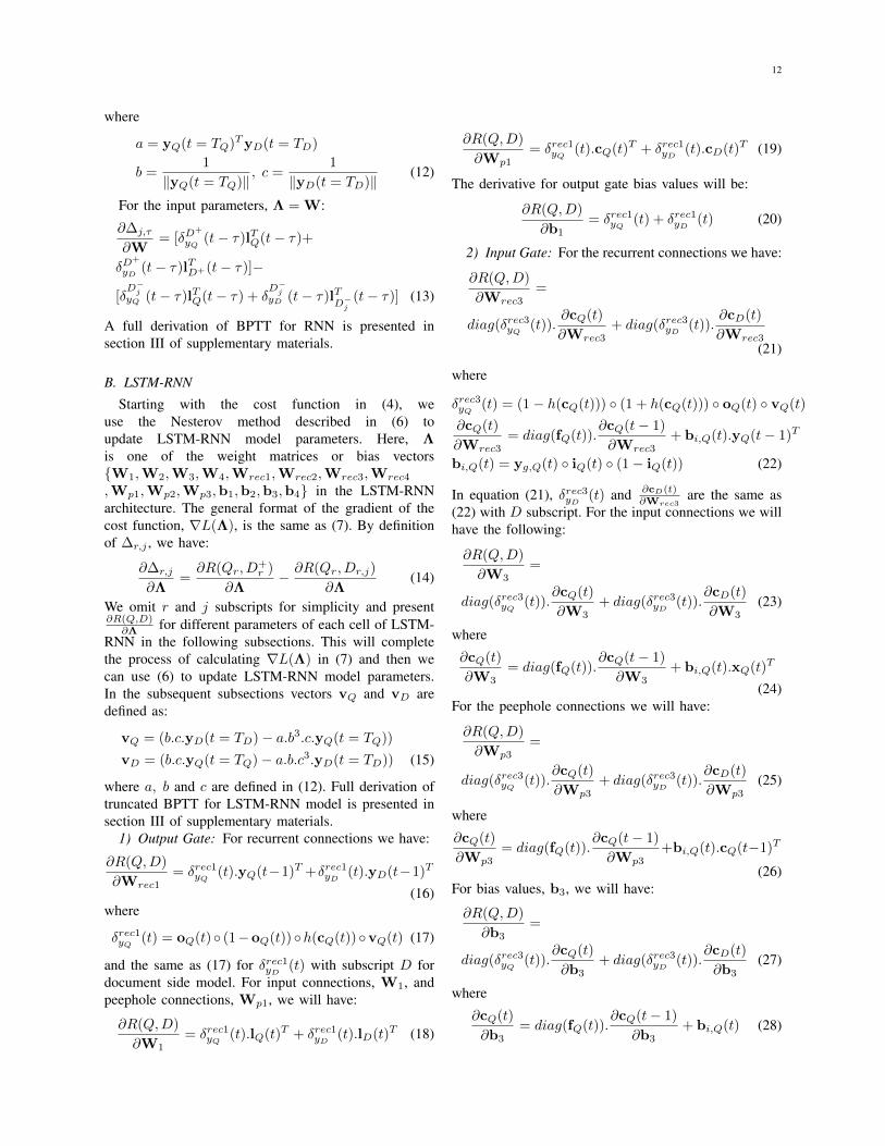
1) Attenuating Unimportant Information: First, weexamine the evolution of the semantic vector and howunimportant words are attenuated. Specifically, we feedthe following input sentences from the test dataset intothe trained LSTM-RNN model:• Query: “hotels in shanghai”• Document: “shanghai hotels accommodation hotel

in shanghai discount and reservation”Activations of input gate, output gate, cell state and theembedding vector for each cell for query and documentare shown in Fig. 4 and Fig. 5, respectively. The verticalaxis is the cell index from 1 to 32, and the horizontalaxis is the word index from 1 to 10 numbered from leftto right in a sequence of words and color codes showactivation values. From Figs.4–5, we make the followingobservations:• Semantic representation y(t) and cell states c(t) are

evolving over time. Valuable context information isgradually absorbed into c(t) and y(t), so that theinformation in these two vectors becomes richerover time, and the semantic information of theentire input sentence is embedded into vector y(t),which is obtained by applying output gates to thecell states c(t).

• The input gates evolve in such a way that itattenuates the unimportant information and de-tects the important information from the input

2 4 6 8 10

5

10

15

20

25

30−0.6

−0.4

−0.2

0

0.2

0.4

(a) i(t)

2 4 6 8 10

5

10

15

20

25

30−0.6

−0.4

−0.2

0

0.2

0.4

(b) c(t)

2 4 6 8 10

5

10

15

20

25

30−0.6

−0.4

−0.2

0

0.2

0.4

(c) o(t)

2 4 6 8 10

5

10

15

20

25

30−0.6

−0.4

−0.2

0

0.2

0.4

(d) y(t)

Fig. 5. Document: “shanghai hotels accommodation hotelin shanghai discount and reservation”. Since the sentence endsat the ninth word, all the values to the right of it are zero (green color).

sentence. For example, in Fig. 5(a), most ofthe input gate values corresponding to word 3,word 7 and word 9 have very small values(light green-yellow color)1, which corresponds tothe words “accommodation”, “discount” and“reservation”, respectively, in the document sen-tence. Interestingly, input gates reduce the effect ofthese three words in the final semantic representa-tion, y(t), such that the semantic similarity betweensentences from query and document sides are notaffected by these words.

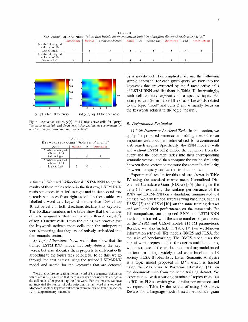
2) Keywords Extraction: In this section, we showhow the trained LSTM-RNN extracts the important in-formation, i.e., keywords, from the input sentences. Tothis end, we backtrack semantic representations, y(t),over time. We focus on the 10 most active cells infinal semantic representation. Whenever there is a largeenough change in cell activation value (y(t)), we assumean important keyword has been detected by the model.We illustrate the result using the above example (“hotelsin shanghai”). The evolution of the 10 most active cellsactivation, y(t), over time are shown in Fig. 6 for thequery and the document sentences.2From Fig. 6, we alsoobserve that different words activate different cells. InTables I–II, we show the number of cells each word

1If this is not clearly visible, please refer to Fig. 1 in section I ofsupplementary materials. We have adjusted color bar for all figures tohave the same range, for this reason the structure might not be clearlyvisible. More visualization examples could also be found in section IVof Supplementary Materials

2Likewise, the vertical axis is the cell index and horizontal axis isthe word index in the sentence.

8

TABLE IIKEY WORDS FOR DOCUMENT: “shanghai hotels accommodation hotel in shanghai discount and reservation”

shanghai hotels accommodation hotel in shanghai discount and reservationNumber of assigned

cells out of 10Left to Right - 4 3 8 1 8 5 3 4

Number of assignedcells out of 10Right to Left 4 6 5 4 5 1 7 5 -

1 2 3

2

4

6

8

10 0

0.02

0.04

0.06

0.08

(a) y(t) top 10 for query

2 4 6 8

2

4

6

8

10 0

0.05

0.1

(b) y(t) top 10 for document

Fig. 6. Activation values, y(t), of 10 most active cells for Query:“hotels in shanghai” and Document: “shanghai hotels accommodationhotel in shanghai discount and reservation”

TABLE IKEY WORDS FOR QUERY: “hotels in shanghai”

Query hotels in shanghaiNumber of assigned

cells out of 10Left to Right - 0 7

Number of assignedcells out of 10Right to Left 6 0 -

activates.3 We used Bidirectional LSTM-RNN to get theresults of these tables where in the first row, LSTM-RNNreads sentences from left to right and in the second rowit reads sentences from right to left. In these tables welabelled a word as a keyword if more than 40% of top10 active cells in both directions declare it as keyword.The boldface numbers in the table show that the numberof cells assigned to that word is more than 4, i.e., 40%of top 10 active cells. From the tables, we observe thatthe keywords activate more cells than the unimportantwords, meaning that they are selectively embedded intothe semantic vector.

3) Topic Allocation: Now, we further show that thetrained LSTM-RNN model not only detects the key-words, but also allocates them properly to different cellsaccording to the topics they belong to. To do this, we gothrough the test dataset using the trained LSTM-RNNmodel and search for the keywords that are detected

3Note that before presenting the first word of the sequence, activationvalues are initially zero so that there is always a considerable change inthe cell states after presenting the first word. For this reason, we havenot indicated the number of cells detecting the first word as a keyword.Moreover, another keyword extraction example can be found in sectionIV of supplementary materials.

by a specific cell. For simplicity, we use the followingsimple approach: for each given query we look into thekeywords that are extracted by the 5 most active cellsof LSTM-RNN and list them in Table III. Interestingly,each cell collects keywords of a specific topic. Forexample, cell 26 in Table III extracts keywords relatedto the topic “food” and cells 2 and 6 mainly focus onthe keywords related to the topic “health”.

B. Performance Evaluation

1) Web Document Retrieval Task: In this section, weapply the proposed sentence embedding method to animportant web document retrieval task for a commercialweb search engine. Specifically, the RNN models (withand without LSTM cells) embed the sentences from thequery and the document sides into their correspondingsemantic vectors, and then compute the cosine similaritybetween these vectors to measure the semantic similaritybetween the query and candidate documents.

Experimental results for this task are shown in TableIV using the standard metric mean Normalized Dis-counted Cumulative Gain (NDCG) [36] (the higher thebetter) for evaluating the ranking performance of theRNN and LSTM-RNN on a standalone human-rated testdataset. We also trained several strong baselines, such asDSSM [3] and CLSM [10], on the same training datasetand evaluated their performance on the same task. Forfair comparison, our proposed RNN and LSTM-RNNmodels are trained with the same number of parametersas the DSSM and CLSM models (14.4M parameters).Besides, we also include in Table IV two well-knowninformation retrieval (IR) models, BM25 and PLSA, forthe sake of benchmarking. The BM25 model uses thebag-of-words representation for queries and documents,which is a state-of-the-art document ranking model basedon term matching, widely used as a baseline in IRsociety. PLSA (Probabilistic Latent Semantic Analysis)is a topic model proposed in [37], which is trainedusing the Maximum A Posterior estimation [38] onthe documents side from the same training dataset. Weexperimented with a varying number of topics from 100to 500 for PLSA, which gives similar performance, andwe report in Table IV the results of using 500 topics.Results for a language model based method, uni-gram

9

TABLE IIIKEYWORDS ASSIGNED TO EACH CELL OF LSTM-RNN FOR DIFFERENT QUERIES OF TWO TOPICS, “FOOD” AND “HEALTH”

Query cell 1 cell 2 cell 3 cell 4 cell 5 cell 6 cell 7 cell 8 cell 9 cell 10 cell 11 cell 12 cell 13 cell 14 cell 15 cell 16al yo yo sauce yo sauce sauce

atkins diet lasagna dietblender recipes

cake bakery edinburgh bakerycanning corn beef hash beef, hash

torre de pizzafamous desserts desserts

fried chicken chicken chickensmoked turkey recipesitalian sausage hoagies sausage

do you get allergy allergymuch pain will after total knee replacement pain pain, knee

how to make whiter teeth make, teeth toillini community hospital community, hospital hospital community

implant infection infection infectionintroductory psychology psychology psychology

narcotics during pregnancy side effects pregnancy pregnancy,effects, during duringfight sinus infections infections

health insurance high blood pressure insurance blood high, bloodall antidepressant medications antidepressant, medications

Query cell 17 cell 18 cell 19 cell 20 cell 21 cell 22 cell 23 cell 24 cell 25 cell 26 cell 27 cell 28 cell 29 cell 30 cell 31 cell 32al yo yo sauce

atkins diet lasagna diet dietblender recipes recipes

cake bakery edinburgh bakery bakerycanning corn beef hash corn, beef

torre de pizza pizza pizzafamous desserts

fried chicken chickensmoked turkey recipes turkey recipesitalian sausage hoagies hoagies sausage sausage

do you get allergymuch pain will after total knee replacement knee replacement

how to make whiter teeth whiterillini community hospital hospital hospital

implant infection infectionintroductory psychology psychology

narcotics during pregnancy side effectsfight sinus infections sinus, infections infections

health insurance high blood pressure high, pressure insurance,highall antidepressant medications antidepressant medications

language model (ULM) with Dirichlet smoothing, arealso presented in the table.

To compare the performance of the proposed methodwith general sentence embedding methods in documentretrieval task, we also performed experiments using twogeneral sentence embedding methods.

1) In the first experiment, we used the method pro-posed in [2] that generates embedding vectorsknown as Paragraph Vectors. It is also known asdoc2vec. It maps each word to a vector and thenuses the vectors representing all words inside acontext window to predict the vector representationof the next word. The main idea in this method isto use an additional paragraph token from previ-ous sentences in the document inside the contextwindow. This paragraph token is mapped to vectorspace using a different matrix from the one used tomap the words. A primary version of this methodis known as word2vec proposed in [39]. The onlydifference is that word2vec does not include theparagraph token.To use doc2vec on our dataset, we first traineddoc2vec model on both train set (about 200,000query-document pairs) and test set (about 900,000query-document pairs). This gives us an embed-ding vector for every query and document in thedataset. We used the following parameters fortraining:• min-count=1 : minimum number of of words

per sentence, sentences with words less thanthis will be ignored. We set it to 1 to makesure we do not throw away anything.

• window=5 : fixed window size explained in[2]. We used different window sizes, it re-sulted in about just 0.4% difference in finalNDCG values.

• size=100 : feature vector dimension. We used400 as well but did not get significantly dif-ferent NDCG values.

• sample=1e-4 : this is the down sampling ratiofor the words that are repeated a lot in corpus.

• negative=5 : the number of noise words, i.e.,words used for negative sampling as explainedin [2].

• We used 30 epochs of training. We ran an ex-periment with 100 epochs but did not observemuch difference in the results.

• We used gensim [40] to perform experiments.

To make sure that a meaningful model is trained,we used the trained doc2vec model to find themost similar words to two sample words in ourdataset, e.g., the words “pizza” and “infection”.The resulting words and corresponding scores arepresented in section V of Supplementary Materi-als. As it is observed from the resulting words,the trained model is a meaningful model and canrecognise semantic similarity.Doc2vec also assigns an embedding vector for

10

each query and document in our test set. We usedthese embedding vectors to calculate the cosinesimilarity score between each query-document pairin the test set. We used these scores to calcu-late NDCG values reported in Table IV for theDoc2Vec model.Comparing the results of doc2vec model withour proposed method for document retrieval taskshows that the proposed method in this papersignificantly outperforms doc2vec. One reason forthis is that we have used a very general sen-tence embedding method, doc2vec, for documentretrieval task. This experiment shows that it isnot a good idea to use a general sentence embed-ding method and using a better task oriented costfunction, like the one proposed in this paper, isnecessary.

2) In the second experiment, we used the Skip-Thought vectors proposed in [6]. During train-ing, skip-thought method gets a tuple (s(t −1), s(t), s(t + 1)) where it encodes the sentences(t) using one encoder, and tries to reconstructthe previous and next sentences, i.e., s(t− 1) ands(t+ 1), using two separate decoders. The modeluses RNNs with Gated Recurrent Unit (GRU)which is shown to perform as good as LSTM.In the paper, authors have emphasized that: ”Ourmodel depends on having a training corpus of con-tiguous text”. Therefore, training it on our trainingset where we barely have more than one sentencein query or document title is not fair. However,since their model is trained on 11,038 books fromBookCorpus dataset [7] which includes about 74million sentences, we can use the trained modelas an off-the-shelf sentence embedding method asauthors have concluded in the conclusion of thepaper.To do this we downloaded their trained mod-els and word embeddings (its size was morethan 2GB) available from “https://github.com/ryankiros/skip-thoughts”. Then we encoded eachquery and its corresponding document title in ourtest set as vector.We used the combine-skip sentence embeddingmethod, a vector of size 4800 × 1, where it isconcatenation of a uni-skip, i.e., a unidirectionalencoder resulting in a 2400 × 1 vector, and a bi-skip, i.e., a bidirectional encoder resulting in a1200 × 1 vector by forward encoder and another1200×1 vector by backward encoder. The authorshave reported their best results with the combine-skip encoder.Using the 4800 × 1 embedding vectors for eachquery and document we calculated the scores and

0 5 10 15 20 25 30 35 40 45 5010

3

104

L(Λ

),logscale

Epoch

LSTM−RNNRNN

Fig. 7. LSTM-RNN compared to RNN during training: The verticalaxis is logarithmic scale of the training cost, L(Λ), in (4). Horizontalaxis is the number of epochs during training.

NDCG for the whole test set which are reportedin Table IV.The proposed method in this paper is perform-ing significantly better than the off-the-shelf skip-thought method for document retrieval task. Nev-ertheless, since we used skip-thought as an off-the-shelf sentence embedding method, its resultis good. This result also confirms that learningembedding vectors using a model and cost functionspecifically designed for document retrieval task isnecessary.

As shown in Table IV, the LSTM-RNN significantlyoutperforms all these models, and exceeds the bestbaseline model (CLSM) by 1.3% in NDCG@1 score,which is a statistically significant improvement. As wepointed out in Sec. V-A, such an improvement comesfrom the LSTM-RNN’s ability to embed the contextualand semantic information of the sentences into a finitedimension vector. In Table IV, we have also presentedthe results when different number of negative samples,n, is used. Generally, by increasing n we expect theperformance to improve. This is because more nega-tive samples results in a more accurate approximationof the partition function in (5). The results of usingBidirectional LSTM-RNN are also presented in TableIV. In this model, one LSTM-RNN reads queries anddocuments from left to right, and the other LSTM-RNNreads queries and documents from right to left. Then theembedding vectors from left to right and right to leftLSTM-RNNs are concatenated to compute the cosinesimilarity score and NDCG values.

A comparison between the value of the cost functionduring training for LSTM-RNN and RNN on the click-through data is shown in Fig. 7. From this figure,we conclude that LSTM-RNN is optimizing the costfunction in (4) more effectively. Please note that allparameters of both models are initialized randomly.

https://github.com/ryankiros/skip-thoughts

https://github.com/ryankiros/skip-thoughts

11

TABLE IVCOMPARISONS OF NDCG PERFORMANCE MEASURES (THE HIGHER

THE BETTER) OF PROPOSED MODELS AND A SERIES OF BASELINEMODELS, WHERE nhid REFERS TO THE NUMBER OF HIDDEN UNITS,ncell REFERS TO NUMBER OF CELLS, win REFERS TO WINDOW SIZE,AND n IS THE NUMBER OF NEGATIVE SAMPLES WHICH IS SET TO 4

UNLESS OTHERWISE STATED. UNLESS STATED OTHERWISE, THERNN AND LSTM-RNN MODELS ARE CHOSEN TO HAVE THE SAME

NUMBER OF MODEL PARAMETERS AS THE DSSM AND CLSMMODELS: 14.4M, WHERE 1M = 106 . THE BOLDFACE NUMBERS

ARE THE BEST RESULTS.Model NDCG NDCG NDCG

@1 @3 @10Skip-Thought 26.9% 29.7% 36.2%off-the-shelf

Doc2Vec 29.1% 31.8% 38.4%ULM 30.4% 32.7% 38.5%BM25 30.5% 32.8% 38.8%

PLSA (T=500) 30.8% 33.7% 40.2%DSSM (nhid = 288/96) 31.0% 34.4% 41.7%

2 LayersCLSM (nhid = 288/96, win=1) 31.8% 35.1% 42.6%2 Layers, 14.4 M parameters

CLSM (nhid = 288/96, win=3) 32.1% 35.2% 42.7%2 Layers, 43.2 M parameters

CLSM (nhid = 288/96, win=5) 32.0% 35.2% 42.6%2 Layers, 72 M parameters

RNN (nhid = 288) 31.7% 35.0% 42.3%1 Layer

LSTM-RNN (ncell = 32) 31.9% 35.5% 42.7%1 Layer, 4.8 M parametersLSTM-RNN (ncell = 64) 32.9% 36.3% 43.4%

1 Layer, 9.6 M parametersLSTM-RNN (ncell = 96) 32.6% 36.0% 43.4%

1 Layer, n = 2LSTM-RNN (ncell = 96) 33.1% 36.5% 43.6%



1 Layer, n = 8Bidirectional LSTM-RNN 33.2% 36.6% 43.6%

(ncell = 96), 1 Layer

VI. CONCLUSIONS AND FUTURE WORK

This paper addresses deep sentence embedding. Wepropose a model based on long short-term memory tomodel the long range context information and embed thekey information of a sentence in one semantic vector. Weshow that the semantic vector evolves over time and onlytakes useful information from any new input. This hasbeen made possible by input gates that detect uselessinformation and attenuate it. Due to general limitationof available human labelled data, we proposed andimplemented training the model with a weak supervisionsignal using user click-through data of a commercial websearch engine.

By performing a detailed analysis on the model, weshowed that: 1) The proposed model is robust to noise,i.e., it mainly embeds keywords in the final semanticvector representing the whole sentence and 2) In the pro-posed model, each cell is usually allocated to keywords

from a specific topic. These findings have been supportedusing extensive examples. As a concrete sample appli-cation of the proposed sentence embedding method, weevaluated it on the important language processing task ofweb document retrieval. We showed that, for this task,the proposed method outperforms all existing state of theart methods significantly.

This work has been motivated by the earlier successesof deep learning methods in speech [41], [42], [43],[44], [45] and in semantic modelling [3], [10], [46],[47], and it adds further evidence for the effectivenessof these methods. Our future work will further extendthe methods to include 1) Using the proposed sentenceembedding method for other important language pro-cessing tasks for which we believe sentence embeddingplays a key role, e.g., the question / answering task. 2)Exploit the prior information about the structure of thedifferent matrices in Fig. 2 to develop a more effectivecost function and learning method. 3) Exploiting atten-tion mechanism in the proposed model to improve theperformance and find out which words in the query arealigned to which words of the document.

APPENDIX AEXPRESSIONS FOR THE GRADIENTS

In this appendix we present the final gradient expres-sions that are necessary to use for training the proposedmodels. Full derivations of these gradients are presentedin section III of supplementary materials.

A. RNN

For the recurrent parameters, Λ = Wrec (we haveommitted r subscript for simplicity):

∂∆j,τ

∂Wrec= [δD

+

yQ (t− τ)yTQ(t− τ − 1)+

δD+

yD (t− τ)yTD+(t− τ − 1)]− [δD−jyQ (t− τ)yTQ(t− τ − 1)

+ δD−jyD (t− τ)yT

D−j(t− τ − 1)] (9)

where D−j means j-th candidate document that is notclicked and

δyQ(t− τ − 1) = (1− yQ(t− τ − 1))◦(1 + yQ(t− τ − 1)) ◦WT

recδyQ(t− τ) (10)

and the same as (10) for δyD (t−τ−1) with D subscriptfor document side model. Please also note that:

δyQ(TQ) = (1− yQ(TQ)) ◦ (1 + yQ(TQ))◦(b.c.yD(TD)− a.b3.c.yQ(TQ)),

δyD (TD) = (1− yD(TD)) ◦ (1 + yD(TD))◦(b.c.yQ(TQ)− a.b.c3.yD(TD)) (11)

12

where

a = yQ(t = TQ)TyD(t = TD)

b =1

‖yQ(t = TQ)‖, c =

1

‖yD(t = TD)‖(12)

For the input parameters, Λ = W:

∂∆j,τ

∂W= [δD

+

yQ (t− τ)lTQ(t− τ)+

δD+

yD (t− τ)lTD+(t− τ)]−

[δD−jyQ (t− τ)lTQ(t− τ) + δ

D−jyD (t− τ)lT

D−j(t− τ)] (13)

A full derivation of BPTT for RNN is presented insection III of supplementary materials.

B. LSTM-RNN

Starting with the cost function in (4), weuse the Nesterov method described in (6) toupdate LSTM-RNN model parameters. Here, Λis one of the weight matrices or bias vectors{W1,W2,W3,W4,Wrec1,Wrec2,Wrec3,Wrec4

,Wp1,Wp2,Wp3,b1,b2,b3,b4} in the LSTM-RNNarchitecture. The general format of the gradient of thecost function, ∇L(Λ), is the same as (7). By definitionof ∆r,j , we have:

∂∆r,j

∂Λ=∂R(Qr, D

+r )

∂Λ− ∂R(Qr, Dr,j)

∂Λ(14)

We omit r and j subscripts for simplicity and present∂R(Q,D)

∂Λ for different parameters of each cell of LSTM-RNN in the following subsections. This will completethe process of calculating ∇L(Λ) in (7) and then wecan use (6) to update LSTM-RNN model parameters.In the subsequent subsections vectors vQ and vD aredefined as:

vQ = (b.c.yD(t = TD)− a.b3.c.yQ(t = TQ))

vD = (b.c.yQ(t = TQ)− a.b.c3.yD(t = TD)) (15)

where a, b and c are defined in (12). Full derivation oftruncated BPTT for LSTM-RNN model is presented insection III of supplementary materials.

1) Output Gate: For recurrent connections we have:

∂R(Q,D)

∂Wrec1= δrec1yQ (t).yQ(t−1)T +δrec1yD (t).yD(t−1)T

(16)where

δrec1yQ (t) = oQ(t) ◦ (1−oQ(t)) ◦h(cQ(t)) ◦vQ(t) (17)

and the same as (17) for δrec1yD (t) with subscript D fordocument side model. For input connections, W1, andpeephole connections, Wp1, we will have:

∂R(Q,D)

∂W1= δrec1yQ (t).lQ(t)T + δrec1yD (t).lD(t)T (18)

∂R(Q,D)

∂Wp1= δrec1yQ (t).cQ(t)T + δrec1yD (t).cD(t)T (19)

The derivative for output gate bias values will be:

∂R(Q,D)

∂b1= δrec1yQ (t) + δrec1yD (t) (20)

2) Input Gate: For the recurrent connections we have:

∂R(Q,D)

∂Wrec3=

diag(δrec3yQ (t)).∂cQ(t)

∂Wrec3+ diag(δrec3yD (t)).

∂cD(t)

∂Wrec3(21)

where

δrec3yQ (t) = (1− h(cQ(t))) ◦ (1 + h(cQ(t))) ◦ oQ(t) ◦ vQ(t)

∂cQ(t)

∂Wrec3= diag(fQ(t)).

∂cQ(t− 1)

∂Wrec3+ bi,Q(t).yQ(t− 1)T

bi,Q(t) = yg,Q(t) ◦ iQ(t) ◦ (1− iQ(t)) (22)

In equation (21), δrec3yD (t) and ∂cD(t)∂Wrec3

are the same as(22) with D subscript. For the input connections we willhave the following:

∂R(Q,D)

∂W3=


∂W3+ diag(δrec3yD (t)).

∂cD(t)

∂W3(23)

where

∂cQ(t)

∂W3= diag(fQ(t)).

∂cQ(t− 1)

∂W3+ bi,Q(t).xQ(t)T

(24)For the peephole connections we will have:

∂R(Q,D)

∂Wp3=


∂Wp3+ diag(δrec3yD (t)).

∂cD(t)

∂Wp3(25)

where

∂cQ(t)

∂Wp3= diag(fQ(t)).

∂cQ(t− 1)

∂Wp3+bi,Q(t).cQ(t−1)T

(26)For bias values, b3, we will have:

∂R(Q,D)

∂b3=


∂b3+ diag(δrec3yD (t)).

∂cD(t)

∂b3(27)

where

∂cQ(t)

∂b3= diag(fQ(t)).

∂cQ(t− 1)

∂b3+ bi,Q(t) (28)

13

3) Forget Gate: For the recurrent connections we willhave:

∂R(Q,D)

∂Wrec2=



∂cD(t)

∂Wrec2(29)

where


∂cQ(t)


∂cQ(t− 1)

∂Wrec2+ bf,Q(t).yQ(t− 1)T

bf,Q(t) = cQ(t− 1) ◦ fQ(t) ◦ (1− fQ(t)) (30)

For input connections to forget gate we will have:

∂R(Q,D)

∂W2=



∂cD(t)

∂W2(31)

where

∂cQ(t)

∂W2= diag(fQ(t)).

∂cQ(t− 1)

∂W2+ bf,Q(t).xQ(t)T

(32)For peephole connections we have:

∂R(Q,D)

∂Wp2=


∂Wp2+ diag(δrec2yD (t)).

∂cD(t)

∂Wp2(33)

where

∂cQ(t)


∂cQ(t− 1)

∂Wp2+bf,Q(t).cQ(t−1)T

(34)For forget gate’s bias values we will have:

∂R(Q,D)

∂b2=



∂cD(t)

∂b2(35)

where

∂cQ(t)

∂b2= diag(fQ(t)).

∂cQ(t− 1)

∂b3+ bf,Q(t) (36)

4) Input without Gating (yg(t)): For recurrent con-nections we will have:

∂R(Q,D)

∂Wrec4=



∂cD(t)

∂Wrec4(37)

where


∂cQ(t)


∂cQ(t− 1)

∂Wrec4+ bg,Q(t).yQ(t− 1)T

bg,Q(t) = iQ(t) ◦ (1− yg,Q(t)) ◦ (1 + yg,Q(t)) (38)

For input connection we have:

∂R(Q,D)

∂W4=



∂cD(t)

∂W4(39)

where

∂cQ(t)

∂W4= diag(fQ(t)).

∂cQ(t− 1)

∂W4+ bg,Q(t).xQ(t)T

(40)For bias values we will have:

∂R(Q,D)

∂b4=



∂cD(t)

∂b4(41)

where

∂cQ(t)

∂b4= diag(fQ(t)).

∂cQ(t− 1)

∂b4+ bg,Q(t) (42)

5) Error signal backpropagation: Error signals areback propagated through time using following equations:

δrec1Q (t− 1) =

[oQ(t− 1) ◦ (1− oQ(t− 1)) ◦ h(cQ(t− 1))]

◦WTrec1.δ

rec1Q (t) (43)

δreciQ (t− 1) = [(1− h(cQ(t− 1))) ◦ (1 + h(cQ(t− 1)))

◦ oQ(t− 1)] ◦WTreci .δ

reciQ (t), for i ∈ {2, 3, 4}

(44)

REFERENCES

[1] I. Sutskever, O. Vinyals, and Q. V. Le, “Sequence to sequencelearning with neural networks,” in Proceedings of Advances inNeural Information Processing Systems, 2014, pp. 3104–3112.

[2] Q. V. Le and T. Mikolov, “Distributed representations of sen-tences and documents,” Proceedings of the 31st InternationalConference on Machine Learning, pp. 1188–1196, 2014.

[3] P.-S. Huang, X. He, J. Gao, L. Deng, A. Acero, and L. Heck,“Learning deep structured semantic models for web searchusing clickthrough data,” in Proceedings of the 22Nd ACMInternational Conference on Conference on Information &Knowledge Management, ser. CIKM ’13. ACM, 2013, pp. 2333–2338.

[4] T. Mikolov, I. Sutskever, K. Chen, G. S. Corrado, and J. Dean,“Distributed representations of words and phrases and their com-positionality,” in Proceedings of Advances in Neural InformationProcessing Systems, 2013, pp. 3111–3119.

[5] T. Mikolov, K. Chen, G. Corrado, and J. Dean, “Efficient esti-mation of word representations in vector space,” arXiv preprintarXiv:1301.3781, 2013.

14

[6] R. Kiros, Y. Zhu, R. Salakhutdinov, R. S. Zemel, A. Torralba,R. Urtasun, and S. Fidler, “Skip-thought vectors,” Advances inNeural Information Processing Systems (NIPS), 2015.

[7] Y. Zhu, R. Kiros, R. Zemel, R. Salakhutdinov, R. Urtasun,A. Torralba, and S. Fidler, “Aligning books and movies: Towardsstory-like visual explanations by watching movies and readingbooks,” arXiv preprint arXiv:1506.06724, 2015.

[8] J. Chung, C. Gulcehre, K. Cho, and Y. Bengio, “Empirical evalu-ation of gated recurrent neural networks on sequence modeling,”NIPS Deep Learning Workshop, 2014.

[9] R. Socher, J. Pennington, E. H. Huang, A. Y. Ng, and C. D.Manning, “Semi-supervised recursive autoencoders for predictingsentiment distributions,” in Proceedings of the Conference onEmpirical Methods in Natural Language Processing, ser. EMNLP’11, 2011, pp. 151–161.

[10] Y. Shen, X. He, J. Gao, L. Deng, and G. Mesnil, “A latent seman-tic model with convolutional-pooling structure for informationretrieval.” CIKM, November 2014.

[11] R. Collobert and J. Weston, “A unified architecture for naturallanguage processing: Deep neural networks with multitask learn-ing,” in International Conference on Machine Learning, ICML,2008.

[12] N. Kalchbrenner, E. Grefenstette, and P. Blunsom, “A convolu-tional neural network for modelling sentences,” Proceedings ofthe 52nd Annual Meeting of the Association for ComputationalLinguistics, June 2014.

[13] B. Hu, Z. Lu, H. Li, and Q. Chen, “Convolutional neuralnetwork architectures for matching natural language sentences,”in Advances in Neural Information Processing Systems 27, 2014,pp. 2042–2050.

[14] J. Zhang, S. Liu, M. Li, M. Zhou, and C. Zong, “Bilingually-constrained phrase embeddings for machine translation,” in Pro-ceedings of the 52nd Annual Meeting of the Association forComputational Linguistics (ACL) (Volume 1: Long Papers), Bal-timore, Maryland, 2014, pp. 111–121.

[15] S. Hochreiter and J. Schmidhuber, “Long short-term memory,”Neural Comput., vol. 9, no. 8, pp. 1735–1780, Nov. 1997.

[16] A. Graves, A. Mohamed, and G. Hinton, “Speech recognitionwith deep recurrent neural networks,” in Proc. ICASSP, Vancou-ver, Canada, May 2013.

[17] H. Sak, A. Senior, and F. Beaufays, “Long short-term memoryrecurrent neural network architectures for large scale acousticmodeling,” in Proceedings of the Annual Conference of Inter-national Speech Communication Association (INTERSPEECH),2014.

[18] K. M. Hermann and P. Blunsom, “Multilingual mod-els for compositional distributed semantics,” arXiv preprintarXiv:1404.4641, 2014.

[19] D. Bahdanau, K. Cho, and Y. Bengio, “Neural machinetranslation by jointly learning to align and translate,” ICLR2015,2015. [Online]. Available: http://arxiv.org/abs/1409.0473

[20] A. Karpathy, J. Johnson, and L. Fei-Fei, “Visualizing and under-standing recurrent networks,” arXiv preprint arXiv:1506.02078,2015.

[21] J. L. Elman, “Finding structure in time,” Cognitive Science,vol. 14, no. 2, pp. 179–211, 1990.

[22] A. J. Robinson, “An application of recurrent nets to phoneprobability estimation,” IEEE Transactions on Neural Networks,vol. 5, no. 2, pp. 298–305, August 1994.

[23] L. Deng, K. Hassanein, and M. Elmasry, “Analysis of the corre-lation structure for a neural predictive model with application tospeech recognition,” Neural Networks, vol. 7, no. 2, pp. 331–339,1994.

[24] T. Mikolov, M. Karafiat, L. Burget, J. Cernocky, and S. Khudan-pur, “Recurrent neural network based language model.” in Proc.INTERSPEECH, Makuhari, Japan, September 2010, pp. 1045–1048.

[25] A. Graves, “Sequence transduction with recurrent neural net-works,” in Representation Learning Workshp, ICML, 2012.

[26] Y. Bengio, N. Boulanger-Lewandowski, and R. Pascanu, “Ad-

vances in optimizing recurrent networks,” in Proc. ICASSP,Vancouver, Canada, May 2013.

[27] J. Chen and L. Deng, “A primal-dual method for training recur-rent neural networks constrained by the echo-state property,” inProceedings of the International Conf. on Learning Representa-tions (ICLR), 2014.

[28] G. Mesnil, X. He, L. Deng, and Y. Bengio, “Investigation ofrecurrent-neural-network architectures and learning methods forspoken language understanding,” in Proc. INTERSPEECH, Lyon,France, August 2013.

[29] L. Deng and J. Chen, “Sequence classification using high-levelfeatures extracted from deep neural networks,” in Proc. ICASSP,2014.

[30] F. A. Gers, J. Schmidhuber, and F. Cummins, “Learning to forget:Continual prediction with lstm,” Neural Computation, vol. 12, pp.2451–2471, 1999.

[31] F. A. Gers, N. N. Schraudolph, and J. Schmidhuber, “Learningprecise timing with lstm recurrent networks,” J. Mach. Learn.Res., vol. 3, pp. 115–143, Mar. 2003.

[32] J. Gao, W. Yuan, X. Li, K. Deng, and J.-Y. Nie, “Smoothingclickthrough data for web search ranking,” in Proceedings ofthe 32Nd International ACM SIGIR Conference on Research andDevelopment in Information Retrieval, ser. SIGIR ’09. NewYork, NY, USA: ACM, 2009, pp. 355–362.

[33] Y. Nesterov, “A method of solving a convex programmingproblem with convergence rate o (1/k2),” Soviet MathematicsDoklady, vol. 27, pp. 372–376, 1983.

[34] I. Sutskever, J. Martens, G. E. Dahl, and G. E. Hinton, “On theimportance of initialization and momentum in deep learning,” inICML (3)’13, 2013, pp. 1139–1147.

[35] R. Pascanu, T. Mikolov, and Y. Bengio, “On the difficulty oftraining recurrent neural networks.” in ICML 2013, ser. JMLRProceedings, vol. 28. JMLR.org, 2013, pp. 1310–1318.

[36] K. Jarvelin and J. Kekalainen, “Ir evaluation methods for re-trieving highly relevant documents,” in Proceedings of the 23rdAnnual International ACM SIGIR Conference on Research andDevelopment in Information Retrieval, ser. SIGIR. ACM, 2000,pp. 41–48.

[37] T. Hofmann, “Probabilistic latent semantic analysis,” in In Proc.of Uncertainty in Artificial Intelligence, UAI99, 1999, pp. 289–296.

[38] J. Gao, K. Toutanova, and W.-t. Yih, “Clickthrough-based latentsemantic models for web search,” ser. SIGIR ’11. ACM, 2011,pp. 675–684.

[39] T. Mikolov, K. Chen, G. Corrado, and J. Dean, “Efficientestimation of word representations in vector space,” inInternational Conference on Learning Representations (ICLR),2013. [Online]. Available: arXiv:1301.3781

[40] R. Rehurek and P. Sojka, “Software Framework for Topic Mod-elling with Large Corpora,” in Proceedings of the LREC 2010Workshop on New Challenges for NLP Frameworks. Val-letta, Malta: ELRA, May 2010, pp. 45–50, http://is.muni.cz/publication/884893/en.

[41] G. E. Dahl, D. Yu, L. Deng, and A. Acero, “Large vocabularycontinuous speech recognition with context-dependent DBN-HMMs,” in Proc. IEEE ICASSP, Prague, Czech, May 2011, pp.4688–4691.

[42] D. Yu and L. Deng, “Deep learning and its applications to sig-nal and information processing [exploratory dsp],” IEEE SignalProcessing Magazine, vol. 28, no. 1, pp. 145 –154, jan. 2011.

[43] G. Dahl, D. Yu, L. Deng, and A. Acero, “Context-dependentpre-trained deep neural networks for large-vocabulary speechrecognition,” Audio, Speech, and Language Processing, IEEETransactions on, vol. 20, no. 1, pp. 30 –42, jan. 2012.

[44] G. Hinton, L. Deng, D. Yu, G. E. Dahl, A. Mohamed, N. Jaitly,A. Senior, V. Vanhoucke, P. Nguyen, T. N. Sainath, and B. Kings-bury, “Deep neural networks for acoustic modeling in speechrecognition: The shared views of four research groups,” IEEESignal Processing Magazine, vol. 29, no. 6, pp. 82–97, November2012.

http://arxiv.org/abs/1409.0473

arXiv:1301.3781

http://is.muni.cz/publication/884893/en

http://is.muni.cz/publication/884893/en

15

[45] L. Deng, D. Yu, and J. Platt, “Scalable stacking and learning forbuilding deep architectures,” in Proc. ICASSP, march 2012, pp.2133 –2136.

[46] J. Gao, P. Pantel, M. Gamon, X. He, L. Deng, and Y. Shen,“Modeling interestingness with deep neural networks,” in Proc.EMNLP, 2014.

[47] J. Gao, X. He, W. tau Yih, and L. Deng, “Learning continuousphrase representations for translation modeling,” in Proc. ACL,2014.

16

2 4 6 8 10

5

10

15

20

25

30−0.6

−0.4

−0.2

0

0.2

0.4

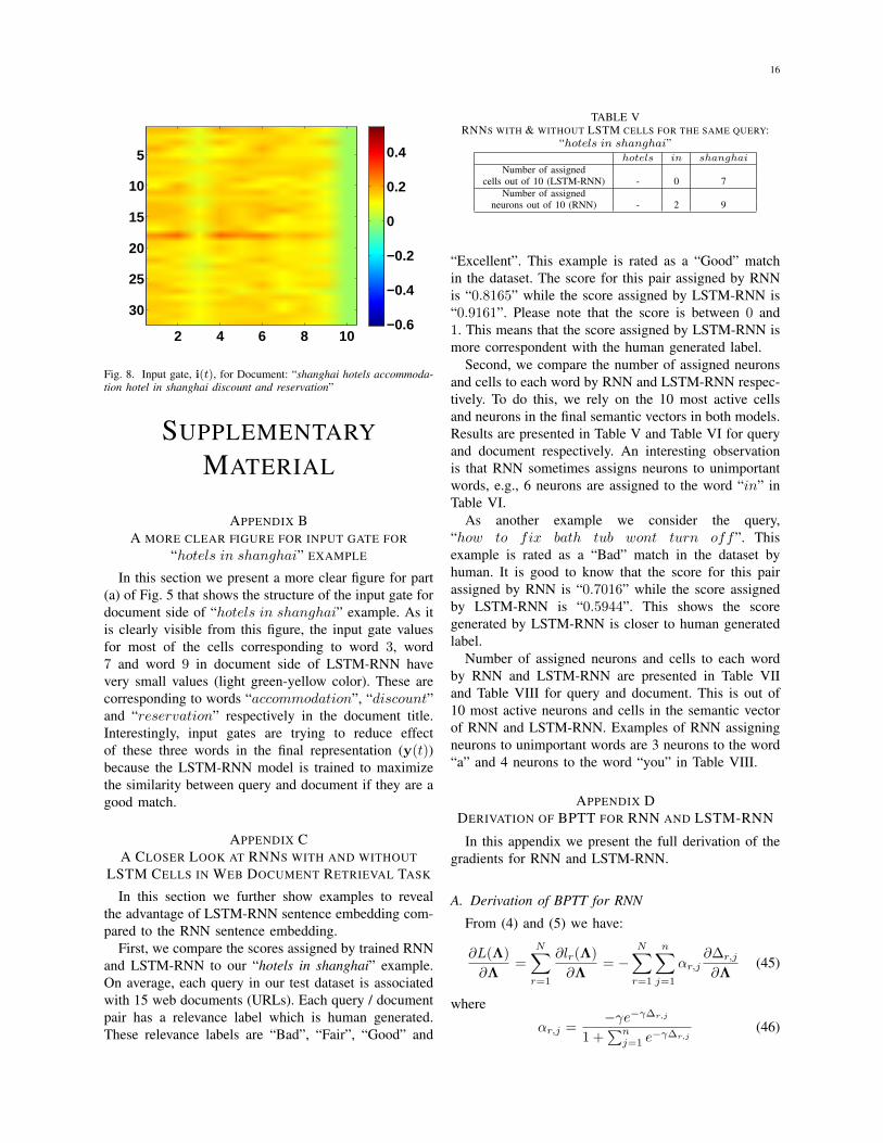
Fig. 8. Input gate, i(t), for Document: “shanghai hotels accommoda-tion hotel in shanghai discount and reservation”

SUPPLEMENTARYMATERIAL

APPENDIX BA MORE CLEAR FIGURE FOR INPUT GATE FOR

“hotels in shanghai” EXAMPLE

In this section we present a more clear figure for part(a) of Fig. 5 that shows the structure of the input gate fordocument side of “hotels in shanghai” example. As itis clearly visible from this figure, the input gate valuesfor most of the cells corresponding to word 3, word7 and word 9 in document side of LSTM-RNN havevery small values (light green-yellow color). These arecorresponding to words “accommodation”, “discount”and “reservation” respectively in the document title.Interestingly, input gates are trying to reduce effectof these three words in the final representation (y(t))because the LSTM-RNN model is trained to maximizethe similarity between query and document if they are agood match.

APPENDIX CA CLOSER LOOK AT RNNS WITH AND WITHOUT

LSTM CELLS IN WEB DOCUMENT RETRIEVAL TASK

In this section we further show examples to revealthe advantage of LSTM-RNN sentence embedding com-pared to the RNN sentence embedding.

First, we compare the scores assigned by trained RNNand LSTM-RNN to our “hotels in shanghai” example.On average, each query in our test dataset is associatedwith 15 web documents (URLs). Each query / documentpair has a relevance label which is human generated.These relevance labels are “Bad”, “Fair”, “Good” and

TABLE VRNNS WITH & WITHOUT LSTM CELLS FOR THE SAME QUERY:

“hotels in shanghai”hotels in shanghai

Number of assignedcells out of 10 (LSTM-RNN) - 0 7

Number of assignedneurons out of 10 (RNN) - 2 9

“Excellent”. This example is rated as a “Good” matchin the dataset. The score for this pair assigned by RNNis “0.8165” while the score assigned by LSTM-RNN is“0.9161”. Please note that the score is between 0 and1. This means that the score assigned by LSTM-RNN ismore correspondent with the human generated label.

Second, we compare the number of assigned neuronsand cells to each word by RNN and LSTM-RNN respec-tively. To do this, we rely on the 10 most active cellsand neurons in the final semantic vectors in both models.Results are presented in Table V and Table VI for queryand document respectively. An interesting observationis that RNN sometimes assigns neurons to unimportantwords, e.g., 6 neurons are assigned to the word “in” inTable VI.

As another example we consider the query,“how to fix bath tub wont turn off”. Thisexample is rated as a “Bad” match in the dataset byhuman. It is good to know that the score for this pairassigned by RNN is “0.7016” while the score assignedby LSTM-RNN is “0.5944”. This shows the scoregenerated by LSTM-RNN is closer to human generatedlabel.

Number of assigned neurons and cells to each wordby RNN and LSTM-RNN are presented in Table VIIand Table VIII for query and document. This is out of10 most active neurons and cells in the semantic vectorof RNN and LSTM-RNN. Examples of RNN assigningneurons to unimportant words are 3 neurons to the word“a” and 4 neurons to the word “you” in Table VIII.

APPENDIX DDERIVATION OF BPTT FOR RNN AND LSTM-RNN

In this appendix we present the full derivation of thegradients for RNN and LSTM-RNN.

A. Derivation of BPTT for RNN

From (4) and (5) we have:

∂L(Λ)

∂Λ=

N∑r=1

∂lr(Λ)

∂Λ= −

N∑r=1

n∑j=1

αr,j∂∆r,j

∂Λ(45)

where

αr,j =−γe−γ∆r,j

1 +∑nj=1 e

−γ∆r,j(46)

17

TABLE VIRNNS WITH & WITHOUT LSTM CELLS FOR THE SAME DOCUMENT: “shanghai hotels accommodation hotel in shanghai discount and

reservation”shanghai hotels accommodation hotel in shanghai discount and reservation

Number of assignedcells out of 10 (LSTM-RNN) - 4 3 8 1 8 5 3 4

Number of assignedneurons out of 10 (RNN) - 10 7 9 6 8 3 2 6

TABLE VIIRNN VERSUS LSTM-RNN FOR QUERY: “how to fix bath tub wont turn off ”

how to fix bath tub wont turn offNumber of assigned

cells out of 10 (LSTM-RNN) - 0 4 7 6 3 5 0Number of assigned

neurons out of 10 (RNN) - 1 10 4 6 2 7 1

TABLE VIIIRNN VERSUS LSTM-RNN FOR DOCUMENT: “how do you paint a bathtub and what paint should . . . ”

how do you paint a bathtub and what paint should you . . .Number of assigned

cells out of 10(LSTM-RNN) - 1 1 7 0 9 2 3 8 4Number of assigned

neurons out of 10(RNN) - 1 4 4 3 7 2 5 4 7

and

∆r,j = R(Qr, D+r )−R(Qr, Dr,j) (47)

We need to find ∂∆r,j

∂Λ for input weights and recurrentweights. We omit r subscript for simplicity.

1) Recurrent Weights:

∂∆j

∂Wrec=∂R(Q,D+)

∂Wrec−∂R(Q,D−j )

∂Wrec(48)

We divide R(D,Q) into three components:

R(Q,D) = yQ(t = TQ)TyD(t = TD)︸︷︷︸a

.

1

‖yQ(t = TQ)‖︸︷︷︸b

.1

‖yD(t = TD)‖︸︷︷︸c

(49)

then

∂R(Q,D)

∂Wrec=

∂a

∂Wrec.b.c︸︷︷︸

D

+ a.∂b

∂Wrec.c︸︷︷︸

E

+

a.b.∂c

∂Wrec︸︷︷︸F

(50)

We have

D =∂yQ(t = TQ)TyD(t = TD).b.c

∂Wrec

=∂yQ(t = TQ)TyD(t = TD).b.c

∂yQ(t = TQ).∂yQ(t = TQ)

∂Wrec+

∂yQ(t = TQ)TyD(t = TD).b.c

∂yD(t = TD).∂yD(t = TD)

∂Wrec

= yD(t = TD).b.c.∂yQ(t = TQ)

∂Wrec+

yQ(t = TQ). (b.c)T︸︷︷︸b.c

.∂yD(t = TD)

∂Wrec(51)

Since f(.) = tanh(.), using chain rule we have

∂yQ(t = TQ)

Wrec=

[(1− yQ(t = TQ)) ◦ (1 + yQ(t = TQ))]yQ(t− 1)T

(52)

and therefore

D = [b.c.yD(t = TD) ◦ (1− yQ(t = TQ))◦(1 + yQ(t = TQ))]yQ(t− 1)T+

[b.c.yQ(t = TQ) ◦ (1− yD(t = TD))◦(1 + yD(t = TD))]yD(t− 1)T (53)

To find E we use following basic rule:

∂

∂x‖x− a‖2 =

x− a

‖x− a‖2(54)

18

Therefore

E = a.c.∂

∂Wrec(‖yQ(t = TQ)‖)−1 =

− a.c.(‖yQ(t = TQ)‖)−2.∂‖yQ(t = TQ)‖

∂Wrec

= −a.c.(‖yQ(t = TQ)‖)−2.yQ(t = TQ)

‖yQ(t = TQ)‖∂yQ(t = TQ)

∂Wrec

= −[a.c.b3.yQ(t = TQ) ◦ (1− yQ(t = TQ))◦(1 + yQ(t = TQ))]yQ(t− 1) (55)

F is calculated similar to (55):

F = −[a.b.c3.yD(t = TD) ◦ (1− yD(t = TD))◦(1 + yD(t = TD))]yD(t− 1) (56)

Considering (50),(53),(55) and (56) we have:

∂R(Q,D)

∂Wrec= δyQ(t)yQ(t− 1)T + δyD (t)yD(t− 1)T

(57)where

δyQ(t = TQ) = (1− yQ(t = TQ)) ◦ (1 + yQ(t = TQ))◦(b.c.yD(t = TD)− a.b3.c.yQ(t = TQ)),

δyD (t = TD) = (1− yD(t = TD)) ◦ (1 + yD(t = TD))◦(b.c.yQ(t = TQ)− a.b.c3.yD(t = TD)) (58)

Equation (58) will just unfold the network one time step,to unfold it over rest of time steps using backpropagationwe have:

δyQ(t− τ − 1) = (1− yQ(t− τ − 1))◦(1 + yQ(t− τ − 1)) ◦WT

recδyQ(t− τ),

δyD (t− τ − 1) = (1− yD(t− τ − 1))◦(1 + yD(t− τ − 1)) ◦WT

recδyD (t− τ) (59)

where τ is the number of time steps that we unfold thenetwork over time which is from 0 to TQ and TD forqueries and documents respectively. Now using (48) wehave:

∂∆j,τ

∂Wrec= [δD

+

yQ (t− τ)yTQ(t− τ − 1)+

δD+

yD (t− τ)yTD+(t− τ − 1)]− [δD−jyQ (t− τ)yTQ(t− τ − 1)

+ δD−jyD (t− τ)yT

D−j(t− τ − 1)] (60)

To calculate final value of gradient we should fold backthe network over time and use (45), we will have:

∂L(Λ)

∂Wrec= −

N∑r=1

n∑j=1

T∑τ=0

αr,j,TD,Q∂∆r,j,τ

∂Wrec︸︷︷︸one large update

(61)

2) Input Weights: Using a similar procedure we willhave the following for input weights:

∂R(Q,D)

∂W= δyQ(t−τ)lQ(t−τ)T+δyD (t−τ)lD(t−τ)T

(62)where

δyQ(t− τ) = (1− yQ(t− τ)) ◦ (1 + yQ(t− τ))◦(b.c.yD(t− τ)− a.b3.c.yQ(t− τ)),

δyD (t− τ) = (1− yD(t− τ)) ◦ (1 + yD(t− τ))◦(b.c.yQ(t− τ)− a.b.c3.yD(t− τ)) (63)

Therefore:∂∆j,τ

∂W=

[δD+

yQ (t− τ)lTQ(t− τ) + δD+

yD (t− τ)lTD+(t− τ)]−

[δD−jyQ (t− τ)lTQ(t− τ) + δ

D−jyD (t− τ)lT

D−j(t− τ)] (64)

and therefore:

∂L(Λ)

∂W= −

N∑r=1

n∑j=1

T∑τ=0

αr,j∂∆r,j,τ

∂W︸︷︷︸one large update

(65)

B. Derivation of BPTT for LSTM-RNN

Following from (50) for every parameter, Λ, inLSTM-RNN architecture we have:

∂R(Q,D)

∂Λ=

∂a

∂Λ.b.c︸︷︷︸

D

+ a.∂b

∂Λ.c︸︷︷︸

E

+ a.b.∂c

∂Λ︸︷︷︸F

(66)

and from (51):

D = yD(t = TD).b.c.∂yQ(t = TQ)

∂Λ+

yQ(t = TQ).b.c.∂yD(t = TD)

∂Λ(67)

From (55) and (56) we have:

E = −a.c.b3.yQ(t = TQ)∂yQ(t = TQ)

∂Λ(68)

F = −a.b.c3.yD(t = TD)∂yD(t = TD)

∂Λ(69)

Therefore∂R(Q,D)

∂Λ= D + E + F =

vQ∂yQ(t = TQ)

∂Λ+ vD

∂yD(t = TD)

∂Λ(70)

where

vQ = (b.c.yD(t = TD)− a.b3.c.yQ(t = TQ))

vD = (b.c.yQ(t = TQ)− a.b.c3.yD(t = TD)) (71)

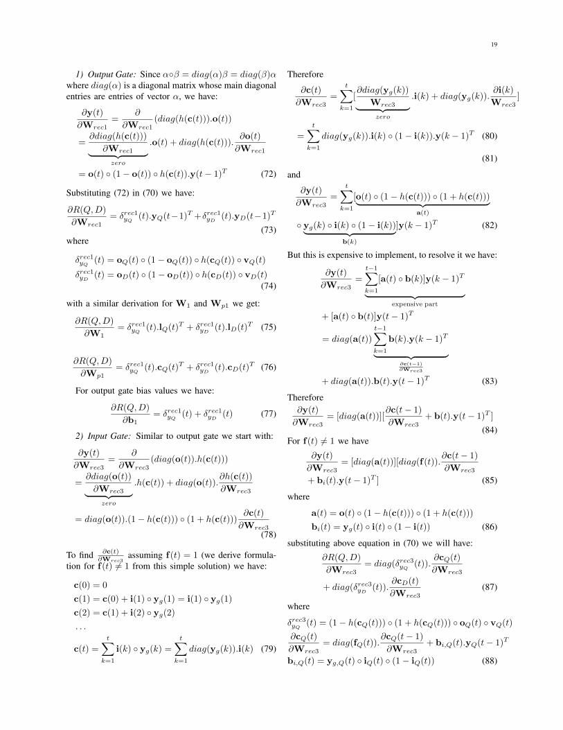
19

1) Output Gate: Since α◦β = diag(α)β = diag(β)αwhere diag(α) is a diagonal matrix whose main diagonalentries are entries of vector α, we have:

∂y(t)

∂Wrec1=

∂

∂Wrec1(diag(h(c(t))).o(t))

=∂diag(h(c(t)))

∂Wrec1︸︷︷︸zero

.o(t) + diag(h(c(t))).∂o(t)

∂Wrec1

= o(t) ◦ (1− o(t)) ◦ h(c(t)).y(t− 1)T (72)

Substituting (72) in (70) we have:

∂R(Q,D)

∂Wrec1= δrec1yQ (t).yQ(t−1)T +δrec1yD (t).yD(t−1)T

(73)where

δrec1yQ (t) = oQ(t) ◦ (1− oQ(t)) ◦ h(cQ(t)) ◦ vQ(t)

δrec1yD (t) = oD(t) ◦ (1− oD(t)) ◦ h(cD(t)) ◦ vD(t)(74)

with a similar derivation for W1 and Wp1 we get:

∂R(Q,D)

∂W1= δrec1yQ (t).lQ(t)T + δrec1yD (t).lD(t)T (75)

∂R(Q,D)

∂Wp1= δrec1yQ (t).cQ(t)T + δrec1yD (t).cD(t)T (76)

For output gate bias values we have:

∂R(Q,D)

∂b1= δrec1yQ (t) + δrec1yD (t) (77)

2) Input Gate: Similar to output gate we start with:

∂y(t)

∂Wrec3=

∂

∂Wrec3(diag(o(t)).h(c(t)))

=∂diag(o(t))

∂Wrec3︸︷︷︸zero

.h(c(t)) + diag(o(t)).∂h(c(t))

∂Wrec3

= diag(o(t)).(1− h(c(t))) ◦ (1 + h(c(t)))∂c(t)

∂Wrec3(78)

To find ∂c(t)∂Wrec3

assuming f(t) = 1 (we derive formula-tion for f(t) 6= 1 from this simple solution) we have:

c(0) = 0

c(1) = c(0) + i(1) ◦ yg(1) = i(1) ◦ yg(1)

c(2) = c(1) + i(2) ◦ yg(2)

. . .

c(t) =

t∑k=1

i(k) ◦ yg(k) =

t∑k=1

diag(yg(k)).i(k) (79)

Therefore

∂c(t)

∂Wrec3=

t∑k=1

[∂diag(yg(k))

Wrec3︸︷︷︸zero

.i(k) + diag(yg(k)).∂i(k)

Wrec3]

=

t∑k=1

diag(yg(k)).i(k) ◦ (1− i(k)).y(k − 1)T (80)

(81)

and

∂y(t)

∂Wrec3=

t∑k=1

[o(t) ◦ (1− h(c(t))) ◦ (1 + h(c(t)))︸︷︷︸a(t)

◦ yg(k) ◦ i(k) ◦ (1− i(k))︸︷︷︸b(k)

]y(k − 1)T (82)

But this is expensive to implement, to resolve it we have:

∂y(t)

∂Wrec3=

t−1∑k=1

[a(t) ◦ b(k)]y(k − 1)T︸︷︷︸expensive part

+ [a(t) ◦ b(t)]y(t− 1)T

= diag(a(t))

t−1∑k=1

b(k).y(k − 1)T︸︷︷︸∂c(t−1)∂Wrec3

+ diag(a(t)).b(t).y(t− 1)T (83)

Therefore∂y(t)

∂Wrec3= [diag(a(t))][

∂c(t− 1)

∂Wrec3+ b(t).y(t− 1)T ]

(84)For f(t) 6= 1 we have

∂y(t)

∂Wrec3= [diag(a(t))][diag(f(t)).

∂c(t− 1)

∂Wrec3

+ bi(t).y(t− 1)T ] (85)

where

a(t) = o(t) ◦ (1− h(c(t))) ◦ (1 + h(c(t)))

bi(t) = yg(t) ◦ i(t) ◦ (1− i(t)) (86)

substituting above equation in (70) we will have:

∂R(Q,D)

∂Wrec3= diag(δrec3yQ (t)).

∂cQ(t)

∂Wrec3

+ diag(δrec3yD (t)).∂cD(t)

∂Wrec3(87)

where


∂cQ(t)


∂cQ(t− 1)

∂Wrec3+ bi,Q(t).yQ(t− 1)T

bi,Q(t) = yg,Q(t) ◦ iQ(t) ◦ (1− iQ(t)) (88)

20

In equation (87), δrec3yD (t) and ∂cD(t)∂Wrec3

are the same as(88) with D subscript. Therefore, update equations forWrec3 are (87), (88) for Q and D and (6).

With a similar procedure for W3 we will have thefollowing:

∂R(Q,D)

∂W3= diag(δrec3yQ (t)).

∂cQ(t)

∂W3


∂W3(89)

where

∂cQ(t)

∂W3= diag(fQ(t)).

∂cQ(t− 1)

∂W3+ bi,Q(t).xQ(t)T

(90)Therefore, update equations for W3 are (89), (90) for Qand D and (6).

For peephole connections we will have:

∂R(Q,D)

∂Wp3= diag(δrec3yQ (t)).

∂cQ(t)

∂Wp3


∂Wp3(91)

where

∂cQ(t)


∂cQ(t− 1)

∂Wp3+bi,Q(t).cQ(t−1)T

(92)Hence, update equations for Wp3 are (91), (92) for Qand D and (6).

Following similar derivation for bias values b3 we willhave:

∂R(Q,D)

∂b3= diag(δrec3yQ (t)).

∂cQ(t)

∂b3


∂b3(93)

where

∂cQ(t)

∂b3= diag(fQ(t)).

∂cQ(t− 1)

∂b3+ bi,Q(t) (94)

Update equations for b3 are (93), (94) for Q and D and(6).

3) Forget Gate: For forget gate, with a similar deriva-tion to input gate we will have

∂y(t)


∂c(t− 1)

∂Wrec2

+ bf (t).y(t− 1)T ] (95)

where

a(t) = o(t) ◦ (1− h(c(t))) ◦ (1 + h(c(t)))

bf (t) = c(t− 1) ◦ f(t) ◦ (1− f(t)) (96)


∂R(Q,D)


∂cQ(t)

∂Wrec2


∂Wrec2(97)

where


∂cQ(t)


∂cQ(t− 1)

∂Wrec2+ bf,Q(t).yQ(t− 1)T

bf,Q(t) = cQ(t− 1) ◦ fQ(t) ◦ (1− fQ(t)) (98)

Therefore, update equations for Wrec2 are (97), (98) forQ and D and (6).

For input weights to forget gate, W2, we have

∂R(Q,D)


∂cQ(t)

∂W2


∂W2(99)

where

∂cQ(t)

∂W2= diag(fQ(t)).

∂cQ(t− 1)

∂W2+ bf,Q(t).xQ(t)T

(100)Therefore, update equations for W2 are (99), (100) forQ and D and (6).

For peephole connections, Wp2, we have

∂R(Q,D)

∂Wp2= diag(δrec2yQ (t)).

∂cQ(t)

∂Wp2


∂Wp2(101)

where

∂cQ(t)


∂cQ(t− 1)

∂Wp2+bf,Q(t).cQ(t−1)T

(102)Therefore, update equations for Wp2 are (101), (102)for Q and D and (6).

Update equations for forget gate bias values, b2, willbe following equations and (6):

∂R(Q,D)


∂cQ(t)

∂b2


∂b2(103)

where

∂cQ(t)

∂b2= diag(fQ(t)).

∂cQ(t− 1)

∂b3+ bf,Q(t) (104)

21

4) Input without Gating (yg(t)): Gradients for yg(t)parameters are as follows:

∂y(t)


∂c(t− 1)

∂Wrec4

+ bg(t).y(t− 1)T ] (105)

where

a(t) = o(t) ◦ (1− h(c(t))) ◦ (1 + h(c(t)))

bg(t) = i(t) ◦ (1− yg(t)) ◦ (1 + yg(t)) (106)


∂R(Q,D)


∂cQ(t)

∂Wrec4


∂Wrec4(107)

where


∂cQ(t)


∂cQ(t− 1)

∂Wrec4+ bg,Q(t).yQ(t− 1)T

bg,Q(t) = iQ(t) ◦ (1− yg,Q(t)) ◦ (1 + yg,Q(t)) (108)

Therefore, update equations for Wrec4 are (107), (108)for Q and D and (6).

For input weight parameters, W4, we have

∂R(Q,D)


∂cQ(t)

∂W4


∂W4(109)

where∂cQ(t)

∂W4= diag(fQ(t)).

∂cQ(t− 1)

∂W4+ bg,Q(t).xQ(t)T

(110)Therefore, update equations for W4 are (109), (110) forQ and D and (6).

Gradients with respect to bias values, b4, are

∂R(Q,D)


∂cQ(t)

∂b4


∂b4(111)

where∂cQ(t)

∂b4= diag(fQ(t)).

∂cQ(t− 1)

∂b4+ bg,Q(t) (112)

Therefore, update equations for b4 are (111), (112) forQ and D and (6). There is no peephole connections foryg(t).

APPENDIX ELSTM-RNN VISUALIZATION

In this appendix we present more examples of LSTM-RNN visualization.

A. LSTM-RNN Semantic Vectors: Another Example

Consider the following example from test dataset:• Query: “how to fix bath tub wont turn off”• Document: “how do you paint a bathtub and whatpaint should you use yahoo answers︸︷︷︸

treated as one word

”

Activations of input gate, output gate, cell state andcell output for each cell for query and document arepresented in Fig.9 and Fig.10 respectively based on atrained LSTM-RNN model.

Three interesting observations from Fig.9 and Fig.10:• Semantic representation y(t) and cell states c(t) are

evolving over time.• In part (a) of Fig.10, we observe that input gate

values for most of the cells corresponding to word3, word 4, word 7 and word 9 in document sideof LSTM-RNN have very small values (light bluecolor). These are corresponding to words “you”,“paint”, “and” and “paint” respectively in thedocument title. Interestingly, input gates are tryingto reduce effect of these words in the final repre-sentation (y(t)) because the LSTM-RNN model istrained to maximize the similarity between queryand document if they are a good match.

• y(t) is used as semantic representation after apply-ing output gate on cell states. Note that valuablecontext information is stored in cell states c(t).

B. Key Word Extraction: Another Example

Evolution of 10 most active cells over time for thesecond example are presented in Fig. 11 for query andFig. 12 for document. Number of assigned cells out of10 most active cells to each word are presented in TableIX and Table X.

APPENDIX FDOC2VEC SIMILARITY TEST

To make sure that a meaningful model is trained,we used the trained doc2vec model to find the mostsimilar words to two sample words in our dataset, thewords “pizza” and “infection”. The resulting words andcorresponding scores are as follows:

print(model.most-similar(’pizza’)) :

[(u’recipes’, 0.9316294193267822),(u’recipe’, 0.9295548796653748),(u’food’, 0.9250608682632446),(u’restaurants’, 0.9223555326461792),(u’bar’, 0.9191627502441406),(u’sabayon’, 0.916868269443512),(u’page’, 0.9160783290863037),

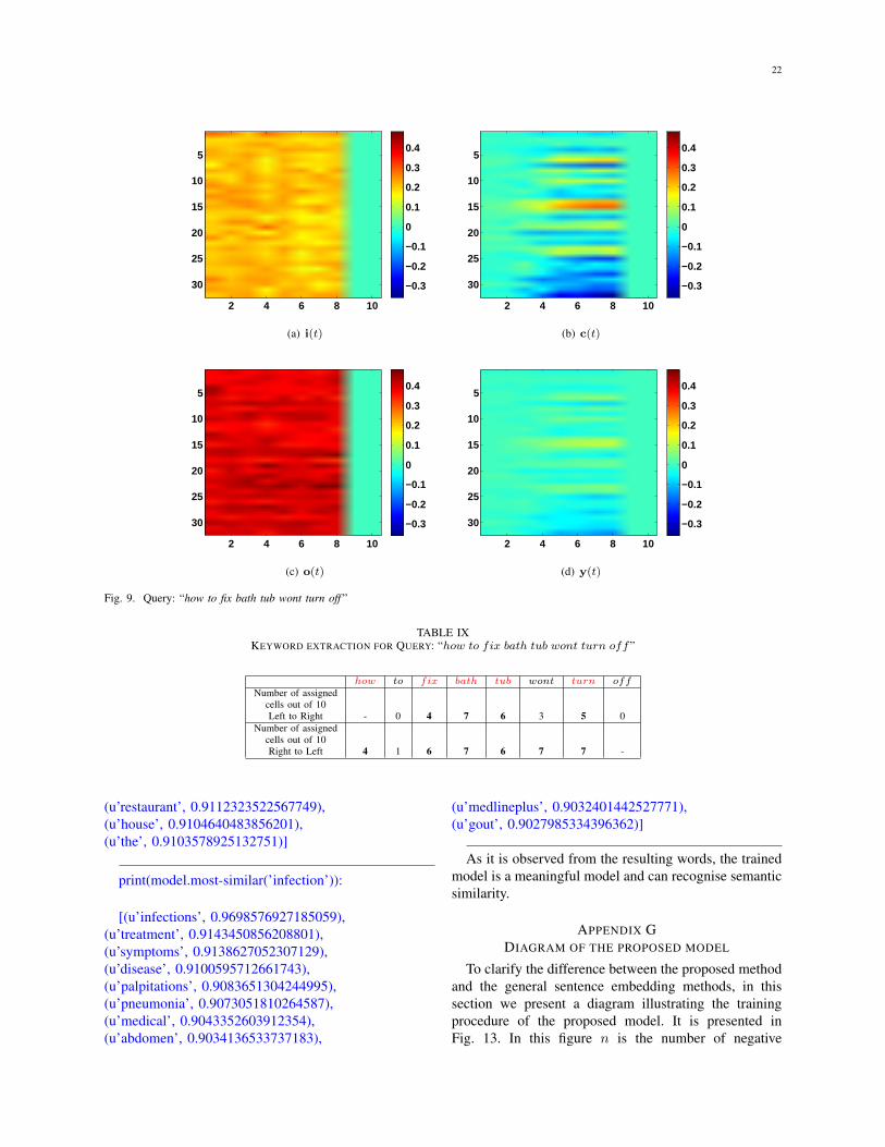
22

2 4 6 8 10

5

10

15

20

25

30 −0.3

−0.2

−0.1

0

0.1

0.2

0.3

0.4

(a) i(t)

2 4 6 8 10

5

10

15

20

25

30 −0.3

−0.2

−0.1

0

0.1

0.2

0.3

0.4

(b) c(t)

2 4 6 8 10

5

10

15

20

25

30 −0.3

−0.2

−0.1

0

0.1

0.2

0.3

0.4

(c) o(t)

2 4 6 8 10

5

10

15

20

25

30 −0.3

−0.2

−0.1

0

0.1

0.2

0.3

0.4

(d) y(t)

Fig. 9. Query: “how to fix bath tub wont turn off ”

TABLE IXKEYWORD EXTRACTION FOR QUERY: “how to fix bath tub wont turn off ”

how to fix bath tub wont turn offNumber of assigned

cells out of 10Left to Right - 0 4 7 6 3 5 0

Number of assignedcells out of 10Right to Left 4 1 6 7 6 7 7 -

(u’restaurant’, 0.9112323522567749),(u’house’, 0.9104640483856201),(u’the’, 0.9103578925132751)]

print(model.most-similar(’infection’)):

[(u’infections’, 0.9698576927185059),(u’treatment’, 0.9143450856208801),(u’symptoms’, 0.9138627052307129),(u’disease’, 0.9100595712661743),(u’palpitations’, 0.9083651304244995),(u’pneumonia’, 0.9073051810264587),(u’medical’, 0.9043352603912354),(u’abdomen’, 0.9034136533737183),

(u’medlineplus’, 0.9032401442527771),(u’gout’, 0.9027985334396362)]

As it is observed from the resulting words, the trainedmodel is a meaningful model and can recognise semanticsimilarity.

APPENDIX GDIAGRAM OF THE PROPOSED MODEL

To clarify the difference between the proposed methodand the general sentence embedding methods, in thissection we present a diagram illustrating the trainingprocedure of the proposed model. It is presented inFig. 13. In this figure n is the number of negative

23

2 4 6 8 10

5

10

15

20

25

300.1

0.12

0.14

0.16

0.18

0.2

0.22

(a) i(t)

2 4 6 8 10

5

10

15

20

25

30 −0.2

−0.1

0

0.1

0.2

0.3

(b) c(t)

2 4 6 8 10

5

10

15

20

25

300.35

0.4

0.45

0.5

0.55

(c) o(t)

2 4 6 8 10

5

10

15

20

25

30 −0.1

−0.05

0

0.05

0.1

(d) y(t)

Fig. 10. Document: “how do you paint a bathtub and what paint should . . . ”

TABLE XKEYWORD EXTRACTION FOR DOCUMENT: “how do you paint a bathtub and what paint should . . . ”

how do you paint a bathtub and what paint should you . . .Number of assigned

cells out of 10Left to Right - 1 1 7 0 9 2 3 8 4

Number of assignedcells out of 10Right to Left 5 9 5 4 8 4 5 5 9 -

(unclicked) documents. The other parameters in thisfigure are similar to those used in Fig. 2 and Fig. 3of the paper.

24

2 4 6 8

2

4

6

8

10 0

0.02

0.04

0.06

0.08

0.1

Fig. 11. Query: “how to fix bath tub wont turn off ”

2 4 6 8 10

2

4

6

8

100

0.02

0.04

0.06

0.08

0.1

Fig. 12. Document: “how do you paint a bathtub and what paint should . . . ”

25

𝑃(𝐷+|𝑄)

Cosine

𝒙(2)

𝑾ℎ

𝒍(2)

LSTM

𝒄(1)

𝒚(2)

𝒙(1)

𝑾ℎ

𝒍(1)

LSTM 𝒚(1)

𝒙(𝑇𝐷2−)

𝑾ℎ

𝒍(𝑇𝐷2−)

LSTM

𝒄(𝑇𝐷2− − 1)

𝒚(𝑇𝐷2−) …

…

Query LSTM

𝑄

Clicked Document LSTM

𝐷+

Unclicked Document LSTM

𝐷1−

… Unclicked Document LSTM

𝐷2−

Unclicked Document LSTM

𝐷𝑛−

𝑃(𝐷1−|𝑄)

Cosine

𝑃(𝐷2−|𝑄)

Cosine

𝑃(𝐷𝑛−|𝑄)

Cosine 𝛿𝑄

𝛿𝐷+

𝛿𝑄 𝛿𝑄 𝛿𝑄

𝛿𝐷1− 𝛿𝐷2− 𝛿𝐷𝑛−

𝛿𝐷2− (𝑇𝐷2−) 𝛿𝐷2− (2) … 𝛿𝐷2− (1)

Semantic representation of the

document

LSTM cells and gates

Backpropagated error signal

Fig. 13. Architecture of the proposed method.

Deep Sentence Embedding Using Long Short-Term Memory ... · 1 Deep Sentence Embedding Using Long...

Documents

Transcript of Deep Sentence Embedding Using Long Short-Term Memory ... · 1 Deep Sentence Embedding Using Long...