Deep learning using EEG spectrograms for prognosis in ... also be used to generate synthetic...

Deep learning using EEG spectrograms for prognosis inidiopathic rapid eye movement behavior disorder (RBD)

Giulio Ruffinia,b,∗, David Ibaneza, Eleni Kroupia, Jean-Francois Gagnonc,e,Marta Castellanoa, Aureli Soria-Frischa

aStarlab Barcelona, Avda. Tibidabo, 47bis, 08035 Barcelona, SpainbNeuroelectrics Corporation, 210 Broadway, Cambridge, MA 02139, USA

cCentre for Advanced Research in Sleep Medicine, Hopital du Sacre-Cœur de Montreal,Montreal, Canada

dDepartment of Neurology, Montreal General Hospital, Montreal, CanadaeDepartment of Psychology, Universite du Quebec a Montreal, Montreal, Canada

fDepartment of Psychiatry, Universite de Montreal

Abstract

REM Behavior Disorder (RBD) is a serious risk factor for neurodegenerative dis-eases such as Parkinson’s disease (PD). In this paper we describe deep learningmethods for RBD prognosis classification from electroencephalography (EEG).We work using a few minutes of eyes-closed resting state EEG data collectedfrom idiopathic RBD patients (121) and healthy controls (HC, 91). At follow-upafter the EEG acquisition (mean of 4 ±2 years), a subset of the RBD patientseventually developed either PD (19) or Dementia with Lewy bodies (DLB, 12),while the rest remained idiopathic RBD. We describe first a deep convolutionalneural network (DCNN) trained with stacked multi-channel spectrograms, treat-ing the data as in audio or image problems where deep classifiers have provenhighly successful exploiting compositional and translationally invariant featuresin the data. Using a multi-layer architecture combining filtering and pooling,the performance of a small DCNN network typically reaches 80% classificationaccuracy. In particular, in the HC vs PD-outcome problem using a single chan-nel, we can obtain an area under the curve (AUC) of 87%. The trained classifiercan also be used to generate synthetic spectrograms to study what aspects ofthe spectrogram are relevant to classification, highlighting the presence of thetabursts and a decrease of power in the alpha band in future PD or DLB patients.For comparison, we study a deep recurrent neural network using stacked long-short term memory network (LSTM) cells [1, 2] or gated-recurrent unit (GRU)cells [3], with similar results. We conclude that, despite the limitations in scopeof this first study, deep classifiers may provide a key technology to analyze theEEG dynamics from relatively small datasets and deliver new biomarkers.

Keywords: Biomarkers, EEG, spectrogram, time-frequency, DCNN, RNN,ConvNET, LSTM, GRU, time-frequency, PD, LBD

∗Corresponding author, [email protected], +1 617-899 6911

Preprint submitted to TBD January 17, 2018

.CC-BY-NC-ND 4.0 International licensepeer-reviewed) is the author/funder. It is made available under aThe copyright holder for this preprint (which was not. http://dx.doi.org/10.1101/240267doi: bioRxiv preprint first posted online Jan. 17, 2018;

http://dx.doi.org/10.1101/240267

http://creativecommons.org/licenses/by-nc-nd/4.0/

1. Introduction

REM Behavior Disorder (RBD) is a serious risk factor for neurodegenerativediseases such as Parkinson’s disease (PD). RBD is a parasomnia characterized byvivid dreaming and dream-enacting behaviors associated with REM sleep with-out muscle atonia [4]. Idiopathic RBD occurs in the absence of any neurologicaldisease or other identified cause, is male-predominant and its clinical course isgenerally chronic progressive [5]. Several longitudinal studies conducted in sleepcenters have shown that most patients diagnosed with the idiopathic form ofRBD will eventually be diagnosed with a neurological disorder such as Parkin-son disease (PD) or dementia with Lewy bodies (DLB) [6, 5, 4]. In essence,idiopathic RBD has been suggested as a prodromal factor of synucleinopathies(PD, DLB and less frequently multiple system atrophy (MSA) [4]).

RBD has an estimated prevalence of 15-60% in PD and has been proposedto define a subtype of PD with relatively poor prognosis, reflecting a brainstem-dominant route of pathology progression (see [7] and references therein) with ahigher risk for dementia or hallucinations. PD with RBD is characterized bymore profound and extensive pathology—not limited to the brainstem—,withhigher synuclein deposition in both cortical and sub-cortical regions.

Electroencephalographic (EEG) and magnetoencephalographic (MEG) sig-nals contain rich information associated with the computational processes inthe brain. To a large extent, progress in their analysis has been driven by thestudy of spectral features in electrode space, which has indeed proven usefulto study the human brain in both health and disease. For example, the “slow-ing down” of EEG is known to characterize neurodegenerative diseases [8, 9].However, neuronal activity exhibits non-linear dynamics and non-stationarityacross temporal scales that cannot be studied well using classical approaches.The field needs novel tools capable of capturing the rich spatio-temporal hierar-chical structures hidden in these signals. Deep learning algorithms are designedfor the task of exploiting compositional structure in data [10]. In past work, forexample, we have used deep feed forward autoencoders for the analysis of EEGdata to address the issue of feature selection, with promising results [11]. Inter-estingly, deep learning techniques, in particular, and artificial neural networksin general are themselves bio-inspired in the brain—the same biological systemgenerating the electric signals we aim to decode. This suggests they should bewell suited for the task.

Deep recurrent neural networks (RNNs), are known to be potentially Turingcomplete [12], although, general RNN architectures are notoriously difficult totrain [2]. In other work we studied a particular class of RNNs called Echo StateNetworks (ESNs) that combine the power of RNNs for classification of temporalpatterns and ease of training [13]. The main idea behind ESNs and other “reser-voir computation” approaches is to use semi-randomly connected, large, fixedrecurrent neural networks where each node/neuron in the reservoir is activatedin a non-linear fashion. The interior nodes with random weights constitute what

2


http://dx.doi.org/10.1101/240267


is called the “dynamic reservoir” of the network. The dynamics of the reservoirprovides a feature representation map of the input signals into a much largerdimensional space (in a sense much like a kernel method). Using such an ESN,we obtained an accuracy of 85% in a binary, class-balanced classification prob-lem (healthy controls versus PD patients) using an earlier, smaller dataset [13].The main limitations of this approach, in our view, were the computational costof developing the dynamics of large random networks and the associated needfor feature selection (e.g., which subset of frequency bands and channels to useas inputs to simplify the computational burden).

In [14], we explored algorithmic complexity metrics of EEG spectrograms,in a further attempt at deriving information from the dynamics of EEG signalsin RBD patients, with good results, indicating that such metrics may be usefulper se for classification or scoring. However, the estimation of such interestingbut ad-hoc metrics may in general lack the power of machine learning methodswhere the relevant features are found directly by the algorithms.

1.1. Deep learning from spectrogram representation

Here we explore first a deep learning approach inspired by recent successesin image classification using deep convolutional neural networks (DCNNs), de-signed to exploit invariances and capture compositional features in the data (seee.g., [2, 10, 12]). These systems have been largely developed to deal with im-age data, i.e., 2D arrays, possibly from different channels, or audio data (as in[15]), and, more recently, with EEG data as well [16, 17]. Thus, inputs to suchnetworks are data cubes (image per channel). In the same vein, we aimed towork here with the spectrograms of EEG channel data, i.e., 2D time-frequencymaps. Such representations represent temporal dynamics as essentially imageswith the equivalent of image depth provided by multiple available EEG channels(or, e.g., current source density maps or cortically mapped quantities from dif-ferent spatial locations). Using such representation, we avoid the need to selectfrequency bands or channels in the process of features selection. This approachessentially treats EEG channel data as an audio file, and our approach mimicssimilar uses of deep networks in that domain.

RNNs can also be used to classify images, e.g., using image pixel rows as timeseries. This is particularly appropriate in our case, given the good performancewe obtained using ESNs on temporal spectral data. We study here also the useof stacked architectures of long-short term memory network (LSTM) or gated-recurrent unit (GRU) cells, which have shown good representational power andcan be trained using backpropagation [1, 3].

Our general assumption is that some relevant aspects in EEG data from ourdatasets are contained in compositional features embedded in the time-frequencyrepresentation. This assumption is not unique to our particular classificationdomain, but should hold of EEG in general. In particular, we expect thatdeep networks may be able to efficiently learn to identify features in the time-frequency domain associated to bursting events across frequency bands thatmay help separate classes, as in “bump analysis” [18]. Bursting events arehypothesized to be representative of transient synchronies of neural populations,

3


http://dx.doi.org/10.1101/240267


which are known to be affected in neurodegenerative diseases such as Parkinson’sor Alzheimer’s disease [19].

Finally, we note that we have made no attempt to optimize these architec-tures. In particular, no fine-tuning of hyper parameters has been carried outusing a validation set approach, something we leave for further work. Our aimhas been to implement a proof of concept of the idea that deep learning ap-proaches can provide value for the analysis of time-frequency representations ofEEG data.

2. EEG dataset

Idiopathic RBD patients (called henceforth RBD for data analysis labeling)and healthy controls were recruited at the Center for Advanced Research in SleepMedicine of the Hopital du Sacre-Cœur de Montral. All patients with full EEGmontage for resting-state EEG recording at baseline and with at least one follow-up examination after the baseline visit were included in the study. The first validEEG for each patient enrolled in the study was considered baseline. Participantsalso underwent a complete neurological examination by a neurologist specializedin movement disorders and a cognitive assessment by a neuropsychologist. Nocontrols reported abnormal motor activity during sleep or showed cognitiveimpairment on neuropsychological testing. The protocol was approved by thehospital’s ethics committee, and all participants gave their written informedconsent to participate. For more details on the protocol and on the patientpopulation statistics (age and gender distribution, follow up time, etc.), see [9].The cohort used here is the same as the one described in [14].

As in previous work [9, 13, 14], the first level data in this study consisted ofresting-state EEG collected from awake patients using 14 scalp electrodes. Therecording protocol consisted of conditions with periods of “eyes open” of variableduration (∼ 2.5 minutes) followed by periods of “eyes closed” in which patientswere not asked to perform any particular task. EEG signals were digitizedwith 16 bit resolution at a sampling rate of 256 S/s. The amplification deviceimplemented hardware band pass filtering between 0.3 and 100 Hz and notchfiltering at 60 Hz to minimize the influence of power line noise. All recordingswere referenced to linked ears. The dataset includes a total of 121 patientsdiagnosed of REM (random eye movement sleep) Behavioral Disorder (RBD)(of which 118 passed the quality tests) and 85 healthy controls (of which only74 provided sufficient quality data) without sleep complaints in which RBD wasexcluded1. EEG data was collected in every patient at baseline, i.e., when theywere still RBD. After 1-10 years of clinical follow-up, 14 patients developedParkinson disease (PD), 13 Lewy body dementia (DLB) and the remaining 91remained idiopathic. Our classification efforts here focuses on the previouslystudied HC vs. PD dual problem.

1We note, however, that several HC were not followed up.

4


http://dx.doi.org/10.1101/240267


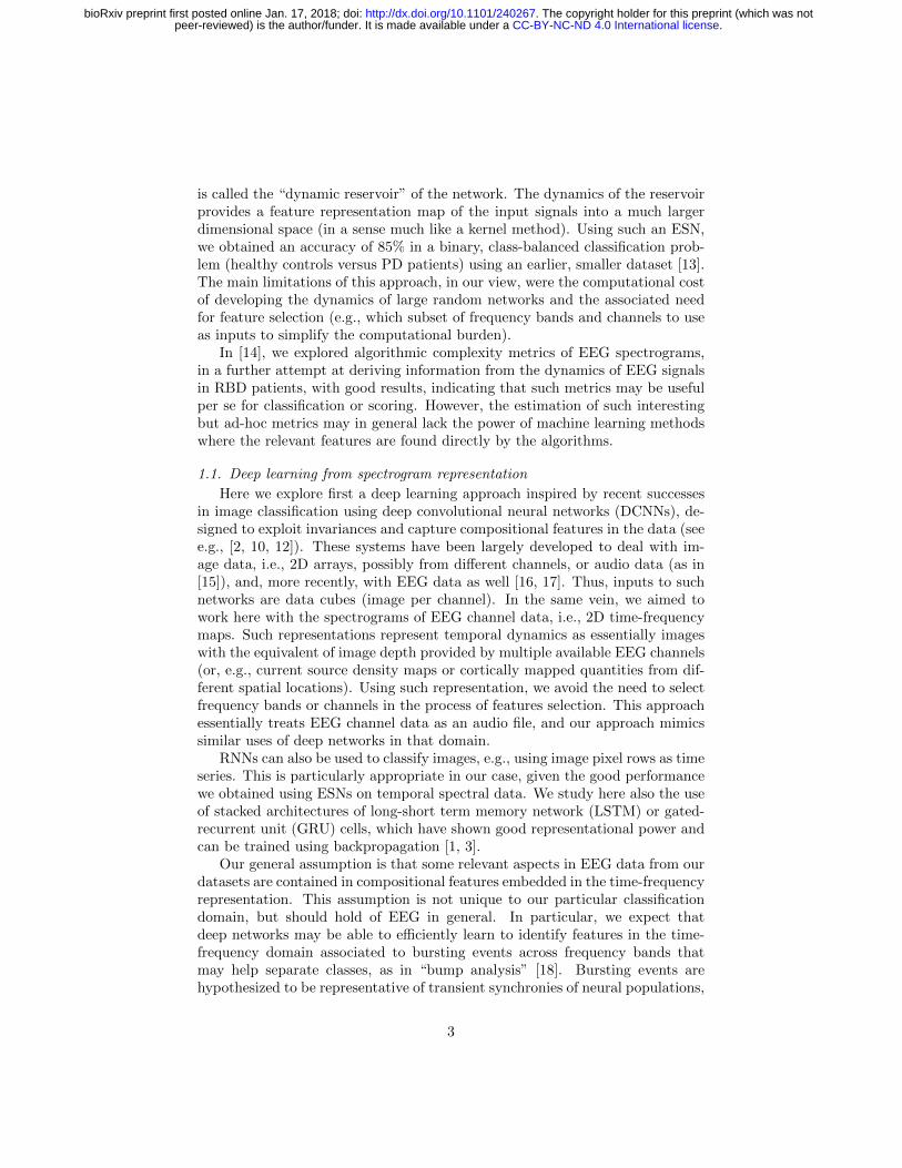
Figure 1: Generation of spectrogram stack for a subject from preprocessed (artifact rejection,referencing, detrending) EEG data.

2.1. Preprocessing and generation of spectrograms

To create the spectrogram dataset (the frames) was processed using Fourieranalysis (FFT) after detrending data blocks of 1 second with a Hann window(FFT resolution is 2 Hz) (see Figure 1). To create the spectrogram frames, 20second 14 channel artifact-free sequences were collected for each subject, using asliding window of 1 second. FFT amplitude bins in the band 4-44 Hz were used.The data frames are thus multidimensional arrays of the form [channels (14)]x [FFTbins (21)] x [Epochs (20)]. The number of frames per subject was setto 148, representing about 2.5 minutes of data. We selected a minimal suitablenumber of frames per subject so that each subject provided the same number offrames. For training, datasets were balanced by random replication of subjectsin the class with fewer subjects. For testing, we used a leave-pair-out strategy,with one subject from each class. Thus, both the training and test sets werebalanced. Finally, the data was centered and normalized to unit variance foreach frequency and channel.

3. Convolutional network architecture

The network (which we call SpectNet), implemented in Tensorflow (Python),is a relatively simple four hidden-layer convolutional net with pooling (see Fig-ure 2). Dropout has been used as the only regularization. All EEG channelsmay be used in the input cube.

Our design philosophy has been to enable the network to find local featuresfirst and create larger views of data with some temporal (but not frequency)shift invariance via max-pooling.

The network has been trained using a cross-entropy loss function to classifyframes (not subjects). It has been evaluated both on frames and, more impor-

5


http://dx.doi.org/10.1101/240267


Figure 2: A. DCNN sample model displaying input, convolution with pooling layers, andsome hidden-unit layers. The output, here for the binary classification problem using one-hotencoding, is a two node layer. B. Synthetic description of architecture. C. Shallow neuralnetwork architecture. D. Deep RNN using LSTM or GRU cells.

tantly, on subjects by averaging subject frame scores and choosing the maximalprobability class, i.e., using a 50% threshold.

For development purposes, we have also tested the performance of thisDCNN on a synthetic dataset consisting of gaussian radial functions randomlyplaced on the spectrogram time axis but with variable stability in frequency,width and amplitude (i.e, by adding some jitter top these parameters). Frameclassification accuracy was high and relatively robust to jitter (∼95-100%, de-pending on parameters).

4. RNN network architecture

The architectures for the RNNs consisted of stacked LSTM [1, 2] or GRUcells [3]. The architecture chosen includes 3 stacked cells, where each cell uses asinput the outputs of the previous one. Each cell typically used about 32 hiddenunits, and dropout was used to regularize it. The performance of LSTM andGRU variants was very similar.

6


http://dx.doi.org/10.1101/240267


Problem N (train/testgroup)

Frametrain/TestACC

Subject TestACC (AUC)

DCNN: HC vs PD 2x73 / 2x1 80% / 73% 80% (87%)

RNN: HC vs PD 2x73 / 2x1 77% / 74% 81% (87%)

DCNN: HC+RBD vs PD+DLB 2x159 / 2x1 73% / 68% 73% (78%)

RNN: HC+RBD vs PD+DLB 2x159 / 2x1 76% / 68% 72% (77%)

Table 1: Performance in different problems using 1 EEG channel (P4). From left to right: Neu-ral Network used and problem addressed (group and whether binary or multiclass); Numberof subjects in training and test sets per group (always balanced); train and test performanceon frames; test accuracy and leave-pair-out (LPO) the area-under-the-curve metric (AUC) onsubjects [20].

5. Classification performance assessment

Classification performance has been evaluated in two ways in a leave-pairout framework (LPO) with a subject from each class. First, by working withbalanced dataset using the accuracy metric (probability of good a classification),and second, by using the area under the curve (AUC) [20]. To map out theclassification performance of the DCNN for different parameter sets, we haveimplemented a set of algorithms in Python (using the Tensorflow module [21])as described by the following pseudocode:

REPEAT N times (experiments):1- Choose (random, balanced) training and test subject sets (leave-pair-out)2- Augment smaller set by random replication of subjects3- Optimize the NN using stochastic gradient descent with frames as inputs4- Evaluate per-frame performance on training and test set5- Evaluate per-subject performance averaging frame outputs

ENDCompute mean and standard deviation of performances over the N experiments

For each frame, the classifier outputs (softmax) the probability of the framebelonging to each class and, as explained above, after averaging over framesper subject we obtain the probability of the subject belonging to each class.Classification is implemented by choosing the class with maximal probability.

The results from classification are shown in Table 1. For comparison, usinga shallow architecture neural network resulted in about 10% less ACC or AUC(in line with our results using SVM classifiers [22, 23]). Figure 6 provides theperformance in the HC-PD problem using different EEG channels.

6. Interpretation

Once a network is trained, it can be used to explore which inputs optimallyexcite network nodes, including the outputs [24]. The algorithm for doing thisis essentially maximizing a particular class score using gradient descent, andstarting from a random noise image. An example of the resulting images us-ing the DCNN above can be seen in Figure 4. This is particularly interestingtechnique, as it provides new insights on pathological features in EEG.

We also checked to see that the trained network was approximately invariantto translation of optimized input images, as expected.

7


http://dx.doi.org/10.1101/240267


7. Discussion

Our results using deep networks are complementary to earlier work with thistype of data using SVMs and ESN/RNNs. However, we deem this approachsuperior for various reasons. First, it largely mitigates the need for featureselection. Secondly, results represent an improvement over our previous efforts,increasing performance by about 5–10% [22, 23].

We note in passing that one of the potential issues with our dataset is thepresence of healthy controls without follow up, which may be a confound. Wehope to remedy this by enlarging our database and by improving our diagnosisand follow up methodologies.

Future steps include the exploration of this approach with larger datasets aswell as continuous refinement of the work done so far, including a more extensiveexploration of network architecture and regularization schemes, including theuse of deeper architectures, improved data augmentation, alternative data seg-mentation and normalization schemes. With regard to data preprocessing, weshould consider improved spectral estimation using advanced techniques suchas state-space estimation and multitapering—as in [25], and working with cor-tically or scalp-mapped EEG data prior creation of spectrograms.

Finally, we note that the techniques used here can be extended to other EEGrelated problems, such as brain computer interfaces or sleep scoring, epilepsyor data cleaning, where the advantages, deep learning approaches may proveuseful as well.

Acknowledgments.

This work has been partially funded by The Michael J. Fox Foundationfor Parkinson’s Research under Rapid Response Innovation Awards 2013. Thedata was collected by Jacques Montplaisir’s team at the Center for AdvancedResearch in Sleep Medicine affiliated to the University of Montreal, Hopital duSacre-Coeur, Montreal and provided within the scope of the aforementionedproject.

References

1. Hochreiter S, Schmidhuber J. Long short-term memory. Neural Computa-tion 1997;9(8):1735–80.

2. Goodfellow I, Bengio Y, Courville A. Deep Learning. MIT Press; 2016.

3. Cho K, van Merrienboer B, Gulcehre C, Bougares F, Schwenk H, Bengio Y.Learning phrase representations using RNN encoder-decoder for statisticalmachine translation. In: Conference on Empirical Methods in Natural Lan-guage Processing (EMNLP 2014), arXiv preprint arXiv:1406.1078. 2014:.

4. Iranzo A, Fernandez-Arcos A, Tolosa E, Serradell M, Molinuevo JL, Vallde-oriola F, Gelpi E, Vilaseca I, Sanchez-Valle R, Llado A, Gaig C, SantamarıaJ. Neurodegenerative disorder risk in idiopathic REM sleep behavior dis-order: Study in 174 patients. PLoS One 2014;9(2).

8


http://dx.doi.org/10.1101/240267


5. Fulda S. Idiopathic REM sleep behavior disorder as a long-term predictorof neurodegenerative disorders. EPMA J 2011;2(4):451–8.

6. Postuma R, Gagnon J, Vendette M, Fantini M, Massicotte-Marquez J, et al. Quantifying the risk of neurodegenerative disease in idiopathic REM sleepbehavior disorder. Neurology 2009;72:1296–300.

7. Kim Y, Kim YE, Park EO, Shin CW, Kim HJ, Jeon B. REM sleep behav-ior disorder portends poor prognosis in Parkinson’s disease: A systematicreview. J Clin Neurosci 2017;.

8. Fantini L, Gagnon J, Petit D, Rompre S, Decary A, Carrier J, MontplaisirJ. Slowing of electroencephalogram in rapid eye movement sleep behaviordisorder. Annals of neurology 2003;53(6):774–80.

9. Rodrigues-Brazete J, Gagnon J, Postuma R, Bertrand J, D Petit MJ. Elec-troencephalogram slowing predicts neurodegeneration in rapid eye move-ment sleep behavior disorder. Neurobiol Aging 2016;37(74-81).

10. Poggio T, Mhaskar H, Rosasco L, Miranda B, Liao Q. Why and when candeep but not shallow networks avoid the curse of dimensionality: a review.Tech. Rep. CBMM Memo 058; Center for Brains, minds and machines;2016.

11. Kroupi E, Soria-Frisch A, Castellano M, nez DI, Montplaisir J, Gagnon JF,Postuma R, Dunne S, Ruffini G. Deep networks using auto-encoders forPD prodromal analysis. In: Proceedings of 1st HBP Student Conference,Vienna. 2017:.

12. Ruffini G. Models, networks and algorithmic complexity.Starlab Technical Note - arXiv:161205627 2016;TN00339(DOI:10.13140/RG.2.2.19510.50249).

13. Ruffini G, Ibanez D, Castellano M, Dunne S, Soria-Frisch A. EEG-drivenRNN classification for prognosis of neurodegeneration in at-risk patients.ICANN 2016 2016;.

14. Ruffini G, Ibanez D, Kroupi E, Gagnon JF, Montplaisir J, Postuma RB,Castellano M, Soria-Frisch A. Algorithmic complexity of EEG for prognosisof neurodegeneration in idiopathic rapid eye movement behavior disorder(RBD). bioRxiv 2017;(200543).

15. van den Oord A, Dieleman S, Schrauwen B. Deep content-based musicrecommendation. In: NIPS. 2013:.

16. Tsinalis O, Matthews PM, Guo Y, Zafeiriou S. Automatic sleep stagescoring with single-channel EEG using convolutional neural networks.arXiv:161001683v1 2016;.

9


http://dx.doi.org/10.1101/240267


17. Vilamala A, Madsen KH, Hansen LK. Deep convolutional neural networksfor interpretable analysis of EEG sleep stage scoring. In: 2017 IEEE In-ternational Workshop On Machine Learning For Signal Processing, Sept.25–28, 2017, Tokyo, Japan. 2017:.

18. Dauwels J, Vialatte F, Musha T, Cichocki A. A comparative study ofsynchrony measures for the early diagnosis of Alzheimer’s disease based onEEG. NeuroImage 2010;(49):668–93.

19. Uhlhaas PJ, Singer W. Neural synchrony in brain review disorders: Rele-vance for cognitive dysfunctions and pathophysiology. Neuron 2006;52:155–68.

20. Airola A, Pahikkala T, Waegeman W, Baets BD, Salakoski T. A compar-ison of AUC estimators in small-sample studies. In: Journal of MachineLearning Research - Proceedings Track. 2010:3–13.

21. Abadi M, et al. . Tensorflow: Large-scale machine learning on heteroge-neous systems. tensorflow.org; 2015.

22. Soria-Frisch A, Marin J, Ibanez DI, Dunne S, Grau C, Ruffini G, Rodrigues-Brazete J, Postuma R, Gagnon JF, Montplaisir J, Pascual-Leone A. Ma-chine learning for a Parkinson’s prognosis and diagnosis system basedon EEG. Proc International Pharmaco-EEG Society Meeting PEG 2014,Leipzig, Germany 2014;.

23. Soria-Frisch A, Marin J, Ibanez D, Dunne S, Grau C, Ruffini G, Rodrigues-Brazete J, Postuma R, Gagnon JF, Montplaisir J, Pascual-Leone A. Eval-uation of EEG biomarkers for Parkinson disease and other Lewy Bodydiseases based on the use of machine learning techniques. in preparation2018;.

24. Simonyan K, Vedaldi A, Zisserman A. Deep inside convolutional networks:Visualising image classification models and saliency maps. arXiv:13126034[csCV] 2014;.

25. Kim SE, Behr MK, Ba D, Brown EN. State-space multitaper time-frequency analysis. PNAS2017;www.pnas.org/cgi/doi/10.1073/pnas.1702877115(1702877115).

10


http://dx.doi.org/10.1101/240267


Figure 3: Sample images produced by maximizing network outputs for a given class. Thisparticular network was trained using P4 electrode data on the problem of HC vs PD+DLB(i.e., HC vs RBDs that will develop synucleinopathy or SNP). The main features are thepresence of 10 Hz bursts in the HC image (top) compared to more persistent 6–8 Hz powerin the pathological spectrogram (bottom). The difference is displayed at the bottom.

11


http://dx.doi.org/10.1101/240267


Figure 4: Sample images produced by maximizing network outputs for a given class. Thisparticular network was trained using P4 electrode channel data on the problem of HC vs PD.The main features are the presence of 10 Hz bursts in the HC image (top) compared to morepersistent 6 Hz power in the pathological spectrogram (bottom). The difference is displayedat the bottom.

12


http://dx.doi.org/10.1101/240267


Figure 5: A. RNN Frame score histogram per class (HC in blue, PD in orange) using a singlechannel. B. Subject mean score. In this particular run, ACC=80%, AUC=87% (both ±1%).There are clearly some subjects that do not classify correctly (this is consistent with DCNNapproach results). The PD outlier is unusual in terms of other metrics, such as slow2fast ratio(EEG slowing) or complexity (see [14]).

13


http://dx.doi.org/10.1101/240267


Figure 6: Top: Accuracy and AUC per channel (averages and SEM over 2000 folds). Occipitaland parietal electrodes provide better discrimination. Top: DCNN architecture. Bottom:RNN.

14


http://dx.doi.org/10.1101/240267


Deep learning using EEG spectrograms for prognosis in ... also be used to generate synthetic...

Documents

Transcript of Deep learning using EEG spectrograms for prognosis in ... also be used to generate synthetic...