Deep Learning Identity-Preserving Face Space

Zhenyao Zhu1,∗ Ping Luo1,3,∗ Xiaogang Wang2 Xiaoou Tang1,3,†1Department of Information Engineering, The Chinese University of Hong Kong2Department of Electronic Engineering, The Chinese University of Hong Kong3Shenzhen Institutes of Advanced Technology, Chinese Academy of Sciences

zz012@ie.cuhk.edu.hk pluo.lhi@gmail.com xgwang@ee.cuhk.edu.hk xtang@ie.cuhk.edu.hk

Abstract

Face recognition with large pose and illumination varia-tions is a challenging problem in computer vision. This pa-per addresses this challenge by proposing a new learning-based face representation: the face identity-preserving(FIP) features. Unlike conventional face descriptors,the FIP features can significantly reduce intra-identityvariances, while maintaining discriminativeness betweenidentities. Moreover, the FIP features extracted from animage under any pose and illumination can be used toreconstruct its face image in the canonical view. Thisproperty makes it possible to improve the performance oftraditional descriptors, such as LBP [2] and Gabor [31],which can be extracted from our reconstructed images inthe canonical view to eliminate variations. In order tolearn the FIP features, we carefully design a deep networkthat combines the feature extraction layers and the recon-struction layer. The former encodes a face image into theFIP features, while the latter transforms them to an imagein the canonical view. Extensive experiments on the largeMultiPIE face database [7] demonstrate that it significantlyoutperforms the state-of-the-art face recognition methods.

1. IntroductionIn many practical applications, the pose and illumination

changes become the bottleneck for face recognition [36].

Many existing works have been proposed to account for

such variations. The pose-invariant methods can be gen-

erally separated into two categories: 2D-based [17, 5, 23]

and 3D-based [18, 3]. In the first category, poses are

either handled by 2D image matching or by encoding a

test image using some bases or exemplars. For example,

∗indicates equal contribution.†This work is supported by the General Research Fund sponsored by

the Research Grants Council of the Kong Kong SAR (Project No. CUHK

416312 and CUHK 416510) and Guangdong Innovative Research Team

Program (No.201001D0104648280).

(a)

(b)

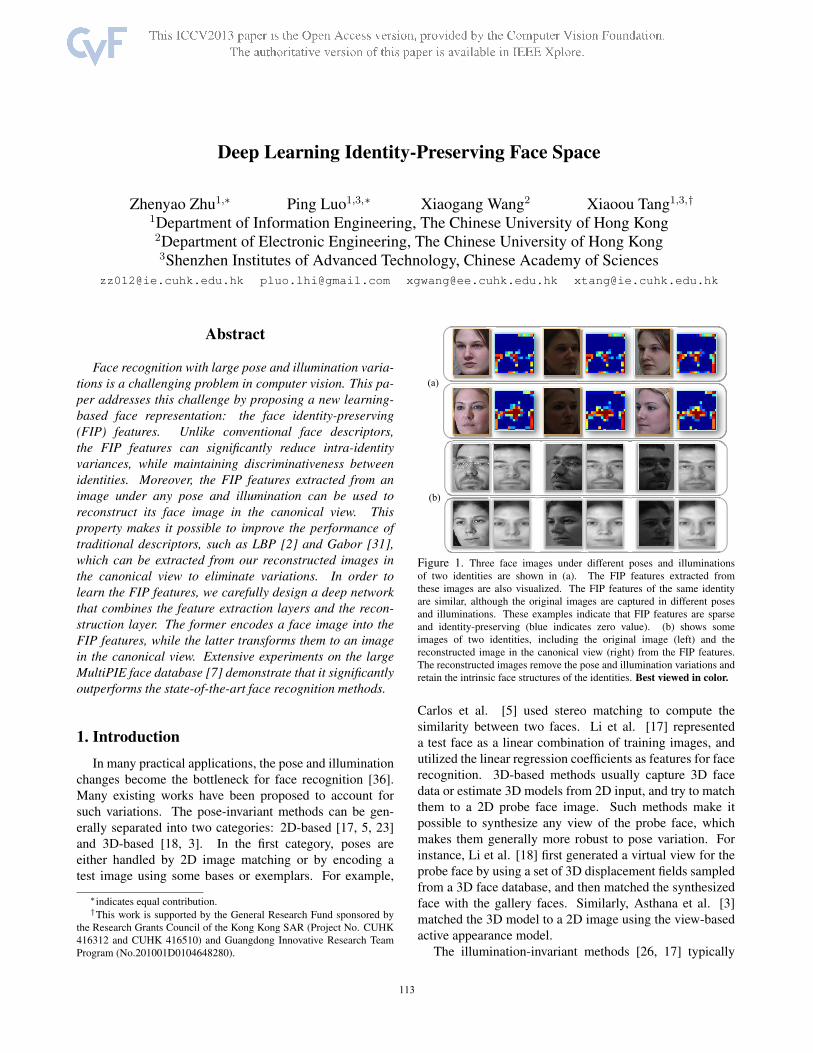
Figure 1. Three face images under different poses and illuminations

of two identities are shown in (a). The FIP features extracted from

these images are also visualized. The FIP features of the same identity

are similar, although the original images are captured in different poses

and illuminations. These examples indicate that FIP features are sparse

and identity-preserving (blue indicates zero value). (b) shows some

images of two identities, including the original image (left) and the

reconstructed image in the canonical view (right) from the FIP features.

The reconstructed images remove the pose and illumination variations and

retain the intrinsic face structures of the identities. Best viewed in color.

Carlos et al. [5] used stereo matching to compute the

similarity between two faces. Li et al. [17] represented

a test face as a linear combination of training images, and

utilized the linear regression coefficients as features for face

recognition. 3D-based methods usually capture 3D face

data or estimate 3D models from 2D input, and try to match

them to a 2D probe face image. Such methods make it

possible to synthesize any view of the probe face, which

makes them generally more robust to pose variation. For

instance, Li et al. [18] first generated a virtual view for the

probe face by using a set of 3D displacement fields sampled

from a 3D face database, and then matched the synthesized

face with the gallery faces. Similarly, Asthana et al. [3]

matched the 3D model to a 2D image using the view-based

active appearance model.

The illumination-invariant methods [26, 17] typically

2013 IEEE International Conference on Computer Vision

1550-5499/13 $31.00 © 2013 IEEE

DOI 10.1109/ICCV.2013.21

113

(a) LBP (b) LE

(c) CRBM (d) FIP

Figure 2. The LBP (a), LE (b), CRBM (c), and FIP (d) features of 50

identities, each of which has 6 images in different poses and illuminations

are projected into two dimensions using Multidimensional scaling (MDS).

Images of the same identity are visualized in the same color. It shows that

FIP has the best representative power. Best viewed in color.

make assumptions about how illumination affects the face

images, and use these assumptions to model and remove

the illumination effect. For example, Wagner et al. [26]

designed a projector-based system to capture images of

each subject in the gallery under a few illuminations, which

can be linearly combined to generate images under arbitrary

illuminations. With this augmented gallery, they adopted

sparse coding to perform face recognition.

The above methods have certain limitations. For ex-

ample, capturing 3D data requires additional cost and

resources [18]. Inferring 3D models from 2D data is an ill-

posed problem [23]. As the statistical illumination models

[26] are often summarized from controlled environment,

they cannot be well generalized in practical applications.

In this paper, unlike previous works that either build

physical models or make statistical assumptions, we

propose a novel face representation, the face identity-

preserving (FIP) features, which are directly extracted

from face images with arbitrary poses and illuminations.

This new representation can significantly remove pose and

illumination variations, while maintaining the discrimina-

tiveness across identities, as shown in Fig.1 (a). Fur-

thermore, unlike traditional face descriptors, e.g. LBP [2],

Gabor [31], and LE [4], which cannot recover the original

images, the FIP features can reconstruct face images in the

frontal pose and with neutral illumination (we call it the

canonical view) of the same identity, as shown in Fig.1 (b).

With this attractive property, the conventional descriptors

and learning algorithms can utilize our reconstructed face

images in the canonical view as input so as to eliminate the

negative effects from poses and illuminations.

Specifically, we present a new deep network to learn

the FIP features. It utilizes face images with arbitrary

pose and illumination variations of an identity as input,

and reconstructs a face in the canonical view of the same

identity as the target (see Fig.3). First, input images are

encoded through feature extraction layers, which have three

locally connected layers and two pooling layers stacked

alternately. Each layer captures face features at a different

scale. As shown in Fig.3, the first locally connected

layer outputs 32 feature maps. Each map has a large

number of high responses outside the face region, which

mainly capture pose information, and some high responses

inside the face region, which capture face structures (red

indicates large response and blue indicates no response).

On the output feature maps of the second locally connected

layer, high responses outside the face region have been

significantly reduced, which indicates that it discards most

pose variations while retain the face structures. The third

locally connected layer outputs the FIP features, which is

sparse and identity-preserving.

Second, the FIP features recover the face image in the

canonical view using a fully-connected reconstruction layer.

As there are large amount of parameters, our network is

hard to train using tranditional training methods [14, 12].

We propose a new training strategy, which contains two

steps: parameter initialization and parameter update. First,

we initialize the parameters based on the least square

dictionary learning. We then update all the parameters by

back-propagating the summed squared reconstruction error

between the reconstructed image and the ground truth.

Existing deep learning methods for face recognition

are generally in two categories: (1) unsupervised learning

features with deep models and then using discriminative

methods (e.g. SVM) for classification [21, 10, 15]; (2)

directly using class labels as supervision of deep models

[6, 24]. In the first category, features related to identity,

poses, and lightings are coupled when learned by deep

models. It is too late to rely on SVM to separate them later.

Our supervised model makes it possible to discard pose and

lighting features from the very bottom layer. In the second

category, a ‘0/1’ class label is a much weaker supervision,

compared with ours using a face image (with thousands

of pixels) of the canonical view as supervision. We

require the deep model to fully reconstruct the face in the

canonical view rather than simply predicting class labels,

and this strong regularization is more effective to avoid

overfitting. This design is suitable for face recognition,

where a canonical view exists. Different from convolutional

neural networks whose filters share weights, our filers

are localized and do not share weights since we assume

different face regions should employ different features.

This work makes three key contributions. (1) We pro-

pose a new deep network that combines the feature extrac-

tion layers and the reconstruction layer. Its architecture is

carefully designed to learn the FIP features. These features

can eliminate the poses and illumination variations, and

114

n2=24 24 32 n2=24 24 32

5 5 Locally Connected and

Pooling

Fully Connected

W1, V1 W3 W4

FIP

W2, V2

Feature Extraction Layers Reconstruction Layer

x0

x1

x2 x3

y y5 5 Locally

Connected and Pooling

5 5 Locally Connected

n0=96 96 n0=96 96

n1=48 48 32

24

24

24

2448

48

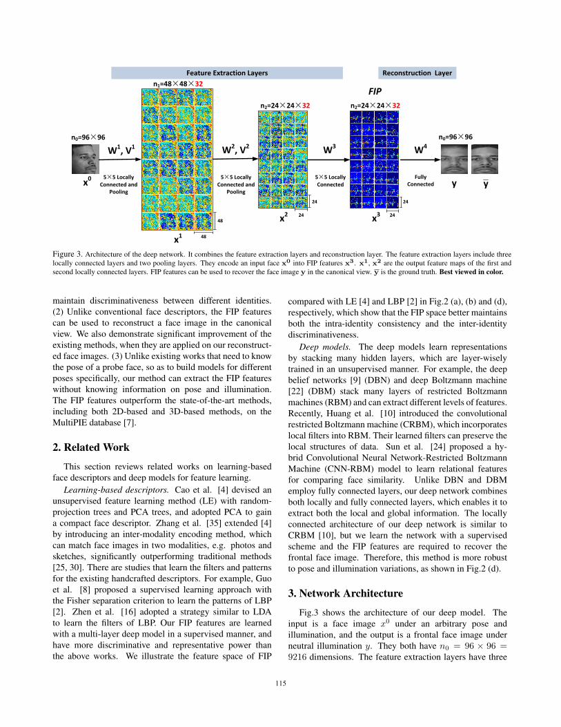
Figure 3. Architecture of the deep network. It combines the feature extraction layers and reconstruction layer. The feature extraction layers include three

locally connected layers and two pooling layers. They encode an input face x0 into FIP features x3. x1, x2 are the output feature maps of the first and

second locally connected layers. FIP features can be used to recover the face image y in the canonical view. y is the ground truth. Best viewed in color.

maintain discriminativeness between different identities.

(2) Unlike conventional face descriptors, the FIP features

can be used to reconstruct a face image in the canonical

view. We also demonstrate significant improvement of the

existing methods, when they are applied on our reconstruct-

ed face images. (3) Unlike existing works that need to know

the pose of a probe face, so as to build models for different

poses specifically, our method can extract the FIP features

without knowing information on pose and illumination.

The FIP features outperform the state-of-the-art methods,

including both 2D-based and 3D-based methods, on the

MultiPIE database [7].

2. Related Work

This section reviews related works on learning-based

face descriptors and deep models for feature learning.

Learning-based descriptors. Cao et al. [4] devised an

unsupervised feature learning method (LE) with random-

projection trees and PCA trees, and adopted PCA to gain

a compact face descriptor. Zhang et al. [35] extended [4]

by introducing an inter-modality encoding method, which

can match face images in two modalities, e.g. photos and

sketches, significantly outperforming traditional methods

[25, 30]. There are studies that learn the filters and patterns

for the existing handcrafted descriptors. For example, Guo

et al. [8] proposed a supervised learning approach with

the Fisher separation criterion to learn the patterns of LBP

[2]. Zhen et al. [16] adopted a strategy similar to LDA

to learn the filters of LBP. Our FIP features are learned

with a multi-layer deep model in a supervised manner, and

have more discriminative and representative power than

the above works. We illustrate the feature space of FIP

compared with LE [4] and LBP [2] in Fig.2 (a), (b) and (d),

respectively, which show that the FIP space better maintains

both the intra-identity consistency and the inter-identity

discriminativeness.

Deep models. The deep models learn representations

by stacking many hidden layers, which are layer-wisely

trained in an unsupervised manner. For example, the deep

belief networks [9] (DBN) and deep Boltzmann machine

[22] (DBM) stack many layers of restricted Boltzmann

machines (RBM) and can extract different levels of features.

Recently, Huang et al. [10] introduced the convolutional

restricted Boltzmann machine (CRBM), which incorporates

local filters into RBM. Their learned filters can preserve the

local structures of data. Sun et al. [24] proposed a hy-

brid Convolutional Neural Network-Restricted Boltzmann

Machine (CNN-RBM) model to learn relational features

for comparing face similarity. Unlike DBN and DBM

employ fully connected layers, our deep network combines

both locally and fully connected layers, which enables it to

extract both the local and global information. The locally

connected architecture of our deep network is similar to

CRBM [10], but we learn the network with a supervised

scheme and the FIP features are required to recover the

frontal face image. Therefore, this method is more robust

to pose and illumination variations, as shown in Fig.2 (d).

3. Network Architecture

Fig.3 shows the architecture of our deep model. The

input is a face image x0 under an arbitrary pose and

illumination, and the output is a frontal face image under

neutral illumination y. They both have n0 = 96 × 96 =9216 dimensions. The feature extraction layers have three

115

locally connected layers and two pooling layers, which

encode x0 into FIP features x3.

In the first layer, x0 is transformed to 32 feature maps

through a weight matrix W 1 that contains 32 sub-matrices

W 1 = [W 11 ;W

12 ; . . . ;W

132], ∀W 1

i ∈ Rn0,n01, each of

which is sparse to retain the locally connected structure

[13]. Intuitively, each row of W 1i represents a small filter

centered at a pixel of x0, so that all of the elements in this

row equal zeros except for the elements belonging to the

filter. As our weights are not shared, the non-zero values of

these rows are not the same2. Therefore, the weight matrix

W 1 results in 32 feature maps {x1i }32i=1, each of which has

n0 dimensions. Then, a matrix V 1, where Vij ∈ {0, 1}encodes the 2D topography of the pooling layer [13], down-

samples each of these feature map to 48 × 48 in order to

reduce the number of parameters need to be learned and

obtain more robust features. Each x1i can be computed as3

x1i = V 1σ(W 1

i x0), (1)

where σ(x) = max(0, x) is the rectified linear function

[19] that is feature-intensity-invariant. So it is robust to

shape and illumination variations. x1 can be obtained by

concatenating all the x1i ∈ R

48×48 together, obtaining a

large feature map in n1 = 48× 48× 32 dimensions.

In the second layer, each x1i is transformed to x2

i 32 sub-

matrices {W 2i }32i=1, ∀W 2

i ∈ R48×48,48×48,

x2i =

32∑j=1

V 2σ(W 2j x

1i ), (2)

where x2i is down-sampled using V 2 to 24×24 dimensions.

Eq.2 means that each small feature map in the first layer is

multiplied by 32 sub-matrices and then summed together.

Here, each sub-matrix has sparse structure as discussed

above. We can reformulate Eq.2 into a matrix form

x2 = V 2σ(W 2x1), (3)

where W 2 = [W 2′1 ; . . . ;W 2′

32], ∀W 2′i ∈ R

48×48,n1 and

x1 = [x11; . . . ;x

132] ∈ R

n1 , respectively. W 2′i is simply

obtained by repeating W 2i for 32 times. Thus, x2 has

n2 = 24× 24× 32 dimensions.

In the third layer, x2 is transformed to x3, i.e. the FIP

features, similar to the second layer, but without pooling.

1In our notation, X ∈ Ra,b means X is a two dimensional matrix

with a rows and b columns. x ∈ Ra×b means x is a vector with a × b

dimensions. Also, [x; y] means that we concatenate vectors or matrices

x and y column-wisely, while [xy] means that we concatenate x and yrow-wisely.

2For the convolutional neural network such as [14], the non-zero values

are the same for each row.3Note that in the conventional deep model [9], there is a bias term b, so

that the output is σ(Wx + b). Since Wx + b can be written as ˜Wx, we

drop the bias term b for simplification.

Thus, x3 is the same size as x2.

x3 = σ(W 3x2), (4)

where W 3 = [W 31 ; . . . ;W

332], ∀W 3

i ∈ R24×24,n2 and x2 =

[x21; . . . ;x

232] ∈ R

n2 , respectively.

Finally, the reconstruction layer transforms the FIP

features x3 to the frontal face image y, through a weight

matrix W 4 ∈ Rn0,n2 ,

y = σ(W 4x3). (5)

4. TrainingTraining our deep network requires estimating all the

weight matrices {W i} as introduced above, which is chal-

lenging because of the millions of parameters. Therefore,

we first initialize the weights and then update them all. V 1

and V 2 are manually defined [13] and fixed.

4.1. Parameter Initialization

We cannot employ RBMs [9] to unsupervised pre-train

the weight matrices, because our input/output data are in

different spaces. Therefore, we devise a supervised method

based on the least square dictionary learning. As shown in

Fig.3, X3 = {x3i }mi=1 are a set of FIP features and Y =

{yi}mi=1 are a set of target images, where m denotes the

number of training examples. Our objective is to minimize

the reconstruction error

arg minW 1,W 2,W 3,W 4

‖ Y − σ(W 4X3) ‖2F , (6)

where ‖ · ‖F is the Frobenius norm. Optimizing Eq.6 is

not trivial because of its nonlinearity. However, we can

initialize the weight matrices layer-wisely as

argminW 1

‖ Y −OW 1X0 ‖2F , (7)

argminW 2

‖ Y − PW 2X1 ‖2F , (8)

argminW 3

‖ Y −QW 3X2 ‖2F , (9)

argminW 4

‖ Y −W 4X3 ‖2F . (10)

In Eq.7, X0 = {x0i }mi=1 is a set of input images. W 1

has been introduced in Sec.3, so that W 1X0 results in 32

feature maps for each input. O is a fixed binary matrix

that sums together the pixels in the same position of these

feature maps, which makes OW 1X0 at the same size as Y .

In Eq.8, X1 = {x1i }mi=1 is a set of outputs of the first locally

connected layer before pooling and P is also a fixed binary

matrix, which sums together the corresponding pixels and

rescales the results to the same size as Y . Q,X2 in Eq.9 are

defined in the same way.

Intuitively, we first directly use X0 to approximate

Y with a linear transform W 1 without pooling. Once

116

W 1 has been initialized, X1 = V 1σ(W 1X0) is used

to approximate Y again with another linear transform,

W 2. We repeat this process until all the matrices have

been initialized. A similar strategy has been adopted

by [33], which learns different levels of representations

with a convolutional architecture. All of the above equa-

tions have closed-form solutions. For example, W 0 =

(OTO)−1(OTY X0T )(X0X0T )−1. The other matrices can

be computed in the same way.

4.2. Parameter Update

We update all the weight matrices after the initialization

by minimizing the loss function of reconstruction error

E(X0;W) =‖ Y − Y ‖2F , (11)

where W = {W 1, . . . ,W 4}. X0 = {x0i }, Y = {yi},

and Y = {yi} are a set of input images, a set of target

images, and a set of reconstructed images, respectively. We

update W using the stochastic gradient descent, in which

the update rule of W i, i = 1 . . . 4, in the k-th iteration is

Δk+1 = 0.9 ·Δk − 0.004 · ε·W ik − ε· ∂E

∂W ik

, (12)

W ik+1 = Δk+1 +W i

k, (13)

where Δ is the momentum variable [20], ε is the learning

rate, and ∂E∂W i = xi−1(ei)T is the derivative, which is

computed as the outer product of the back-propagation error

ei and the feature of the previous layer xi−1. In our deep

network, there are three different expressions of ei. First,

for the transformation layer, e4 is computed based on the

derivative of the linear rectified function [19]

e4j =

{[y − y]j , δ4j > 00, δ4j ≤ 0

, (14)

where δ4j = [W 4x3]j . [·]j denotes the j-th element of a

vector.

Similarly, back-propagation error for e3 is computed as

e3j =

{[W 4T e4]j , δ3j > 00, δ3j ≤ 0

, (15)

where δ3j = [W 3x2]j .

We compute e1 and e2 in the same way as e3 since they

both adopt the same activation function. There is a slight

difference due to down-sampling. For these two layers, we

must up-sample the corresponding back-propagation error eso that it has the same dimensions as the input feature. This

strategy has been introduced in [14]. We need to enforce the

weight matrices to have locally connected structures after

each gradient step as introduced in [12]. We implement this

by setting the corresponding matrix elements to zeros, if

there supposed to be no connections.

5. ExperimentsWe conduct two sets of experiments. Sec.5.1 compares

with state-of-the-art methods and learning-based descrip-

tors. Sec.5.2 demonstrates that classical face recognition

methods can be significantly improved when applied on our

reconstructed face images in the canonical view.

Dataset. To extensively evaluate our method under

different poses and illuminations, we select the MultiPIE

face database [7], which contains 754,204 images of 337

identities. Each identity has images captured under 15

poses and 20 illuminations. These images were captured

in four sessions during different periods. Like the previous

methods [3, 18, 17], we evaluate our algorithm on a subset

of the MultiPIE database, where each identity has images

from all the four sections under seven poses from yaw

angles −45◦ ∼ +45◦, and 20 illuminations marked as ID

00-19 in MultiPIE. This subset has 128,940 images.

5.1. Face Recognition

The existing works conduct experiments on MultiPIE

with three different settings: Setting-I was introduced in

[3, 18, 34]; Setting-II and Setting-III were introduced in

[17]. We describe these settings below.

Setting-I and Setting-II only adopt images with differ-

ent poses, but with neutral illumination marked as ID 07.

They evaluate robustness to pose variations. For Setting-I,

the images of the first 200 identities in all the four sessions

are chosen for training, and the images of the remaining

137 identities for test. During test, one frontal image (i.e.

0◦) of each identity in the test set is selected to the gallery,

so there are 137 gallery images in total. The remaining

images from −45◦ ∼ +45◦ except 0◦ are selected as

probes. For Setting-II, only the images in session one are

used, which only has 249 identities. The images of the

first 100 identities are for training, and the images of the

remaining 149 identities for test. During test, one frontal

image of each identity in the test set is selected in the

gallery. The remaining images from −45◦ ∼ +45◦ except

0◦ are selected as probes.

Setting-III also adopts images in session one for training

and test, but it utilizes the images under all the 7 poses

and 20 illuminations. This is to evaluate the robustness

when both pose and illumination variations are present. The

selection of probes and gallery are the same as Setting-II.

We evaluate both the FIP features and the reconstructed

images using the above three settings. Face images are

roughly aligned according to the positions of eyes, and

rescaled to 96×96. They are converted to grayscale images.

The mean value over the training set is subtracted from

each pixel. For each identity, we use the images with

6 poses ranging from −45◦ ∼ +45◦ except 0◦, and 19

illuminations marked as ID 00-19 except 07, as input to

train our deep network. The reconstruction target is the

117

−45◦ −30◦ −15◦ +15◦ +30◦ +45◦ Avg Pose

LGBP[34] 37.7 62.5 77 83 59.2 36.1 59.3 �

VAAM[3] 74.1 91 95.7 95.7 89.5 74.8 86.9 �

FA-EGFC[18] 84.7 95 99.3 99 92.9 85.2 92.7 �

SA-EGFC[18] 93 98.7 99.7 99.7 98.3 93.6 97.2 �

LE[4]+LDA 86.9 95.5 99.9 99.7 95.5 81.8 93.2 �

CRBM[10]+LDA 80.3 90.5 94.9 96.4 88.3 75.2 87.6 �

FIP+LDA 93.4 95.6 100.0 98.5 96.4 89.8 95.6 �

RL+LDA 95.6 98.5 100.0 99.3 98.5 97.8 98.3 �

Table 1. Recognition rates under Setting-I. The first and the second

highest rates are highlighted. “�” indicates the method needs to know

the pose; “×”, otherwise.

−45◦ −30◦ −15◦ +15◦ +30◦ +45◦ Avg Pose

LE[4]+�2 63.0 90.0 95.0 95.0 90.0 61.5 82.4 �

CRBM[10]+�2 59.9 68.5 94.9 83.2 88.3 66.4 74.7 �

FIP+�2 78.6 87.9 94.9 96.1 91.8 80.8 88.3 �

RL+�2 94.9 94.2 98.5 99.3 98.5 84.0 94.9 �

Table 2. Recognition rates under Setting-I. The proposed features are

compared with LE and CRBM using only the �2 distance for face

recognition. The first and the second highest rates are highlighted. “�”

indicates the method needs to know the pose; “×”, otherwise.

image captured in 0◦ under neutral illumination (ID 07).

In the test stage, in order to better demonstrate the proposed

methods, we directly adopt the FIP and the reconstructed

images (denoted as RL) as features for face recognition.

5.1.1 Results of Setting-IIn this setting, we show superior results in Table 1, where

the FIP and RL features are compared with four methods,

including LGBP [34], VAAM [3], FA-EGFC [18], and SA-

EGFC [18], and two learning-based descriptors, including

LE [4] and CRBM [10]. As discussed in Sec.1, LGBP

is a 2D-based method, while VAAM, FA-EGFC, and SA-

EGFC used 3D face models. We apply LDA on LE, CRBM,

FIP, and RL to obtain compact features. Note that LGBP,

VAAM, and SA-EGFC need to know the pose of a probe,

which means that they build different models to account

for different poses specifically. We do not need to know

the pose of the probe, since our deep network can extract

FIP features and reconstruct the face image in the canonical

view given a probe under any pose and any illumination.

This is one of our advantages over existing methods.

Several observations can be made from Table 1. First,

RL performs best on the averaged recognition rates and five

poses. The improvement is larger for larger pose variations.

It is interesting to note that RL even outperforms all the

3D-based models, which verifies that our reconstructed face

images in the canonical view are of high quality and robust

to pose changes. Fig.4 shows several reconstructed images,

indicating that RL can effectively remove the variations

of poses and illuminations, while still retains the intrinsic

shapes and structures of the identities.

−45◦ −30◦ −15◦ +15◦ +30◦ +45◦ Avg Pose

Li [17] 97.0 97.0 100.0 100.0 97.0 92.0 96.8 �

RL+LDA 97.8 98.6 100.0 100.0 98.6 98.4 98.4 �

Table 3. Recognition rates of RL+LDA compared with Li [17] under

Setting-II. “�” indicates the method needs to know the pose; “×”,

otherwise.

Recognition Rates on Different Poses

−45◦ −30◦ −15◦ +15◦ +30◦ +45◦ Avg Pose

Li [17] 63.5 69.3 79.7 75.6 71.6 54.6 69.3 �

RL+LDA 67.1 74.6 86.1 83.3 75.3 61.8 74.7 �

Recognition Rates on Different Illuminations

00 01 02 03 04 05 06

Li [17] 51.5 49.2 55.7 62.7 79.5 88.3 97.5

RL+LDA 72.8 75.8 75.8 75.7 75.7 75.7 75.7

08 09 10 11 12 13 14

Li [17] 97.7 91.0 79.0 64.8 54.3 47.7 67.3

RL+LDA 75.7 75.7 75.7 75.7 75.7 75.7 73.415 16 17 18 19 Avg.

Li [17] 67.7 75.5 69.5 67.3 50.8 69.3

RL+LDA 73.4 73.4 73.4 72.9 72.9 74.7Table 4. Recognition rates of RL+LDA compared with Li [17] under

Setting-III. “�” indicates the method needs to know the pose; “×”,

otherwise.

Second, FIP features are better than the two learning-

based descriptors and the other three methods except SA-

EGFC, which used the 3D model and required the pose of

the probe. We further report the results of FIP compared

with LE and CRBM using only �2 distance in Table 2 .

The RL and FIP outperform the above two learning based

features, especially when large pose variations are present.

Third, although FIP does not exceed RL, its still a

valuable representation, because it has the sparse property

and can reconstruct RL efficiently and losslessly.

5.1.2 Results of Setting-II and Setting-III

Li et al. [17] evaluated on these two settings and reported

the state-of-the-art results. Setting-II covers only pose

variations and Setting-III covers both pose and illumination

variations.

For Setting-II, the results of RL+LDA compared with

[17] are reported in Table 3, which shows that RL obtains

the best results on all the poses. Note that the poses of

probes in [17] are assumed to be given, which means they

trained a different model for each pose separately. [17]

did not report detailed recognition rates when the poses of

the probes are unknown, except for describing a 20-30%decline of the overall recognition rate.

For Setting-III, RL+LDA is compared with [17] on

images with both pose and illumination variations. Table

4 reports that our approach achieves better results on all

the poses and illuminations. The recognition rate under a

pose is the averaged result over all the possible illumina-

tions. Similarly, the recognition rate under one illumination

118

condition is the averaged result of all the possible poses. We

observe that the performance of RL+LDA under different

illuminations is close because RL can well remove the

effect of different types of illuminations.

5.2. Improve Classical Face Recognition Methods

In this section, we will show that the conventional feature

extraction and dimension reduction methods in the face

recognition literature, such as LBP [2], Gabor [31], PCA

[11], LDA [1], and Sparse Coding (SC) [32], can achieve

significant improvement when they adopt our reconstructed

images as input.

We conduct three experiments using the training/testing

data of Setting-I. First, we show the advantage of our

reconstructed images in the canonical view over the original

images. Second, we show the improvements of Gabor when

it is extracted on our reconstructed images. Third, we show

that LBP can be improved as well.

In the first experiment, �2 distance, SC, PCA, LDA, and

PCA+LDA are directly applied on the raw pixels of the

original images and our reconstructed images, respectively.

The recognition rates are reported in Fig.5(a), where the

results on the original images and the reconstructed images

are illustrated as solid bars (front) and hollow bars (back).

We observe that each of the above methods can be improved

at least 30% on average. They can achieve relatively high

performance on different poses, because our reconstruction

layer can successfully recover the frontal face image. For

example, the recognition rates of SC on different poses

using the original images are 20.9%, 43.6%, 65.0%, 66.1%,

38.3%, and 26.9%, respectively, while 92.7%, 97.1%,

97.8%, 98.5%, 97.8%, and 81.8%, respectively, using the

reconstructed images.

In the second experiment, we extract Gabor features on

both the original images and reconstructed images. We

observe large improvements by using the reconstructed

images. Specifically, for each image in 96× 96, we evenly

select 11 × 10 keypoints and apply 40 Gabor kernels (5

scales × 8 orientations) on each of these keypoints. We

again use the �2 distance, PCA, LDA, and PCA+LDA for

face recognition. The results are shown in Fig.5(b).

In the third experiment, we extract LBP features on both

original images and reconstructed images. Specifically, we

divide each 96 × 96 image into 12 × 12 cells, and the 59

uniform binary patterns are computed in each cell. We

then adopt the χ2 distance, PCA, LDA, and PCA+LDA for

face recognition. Fig.5(c) shows that LBP combined with

all these methods can also be significantly improved. For

instance, the averaged recognition rate of LBP+χ2 using the

original images is 75.9%, and the corresponding accuracy

on our reconstructed images, i.e. RL+LBP+χ2, is 96.5%,

which is better than 94.9% of RL+�2 in Table 2.

0102030405060708090

100

-45 -30 -15 +15 +30 +45

Reco

gniti

on R

ate(

%)

Probe Pose( )NN Sparse Coding PCA LDA PCA+LDA

(a) Pixels

0102030405060708090

100

-45 -30 -15 +15 +30 +45

Reco

gniti

on R

ate(

%)

Probe Pose( )Gabor+NN Gabor+PCA Gabor+LDA Gabor+PCA+LDA

(b) Gabor descriptors

0102030405060708090

100

-45 -30 -15 +15 +30 +45

Reco

gniti

on R

ate(

%)

Probe Pose( )LBP+NN LBP+PCA LBP+LDA LBP+PCA+LDA

(c) LBP descriptors

Figure 5. The conventional face recognition methods can be improved

when they are applied on our reconstructed images. The results of three

descriptors (pixel intensity, Gabor, and LBP) and four face recognition

methods (�2 or χ2 distance, sparse coding (SC), PCA, and LDA) are

reported in (a), (b) and (c), respectively. The hollow bars are the

performance of these methods applied on our reconstructed images, while

the solid bars are on the original images.

6. ConclusionWe have proposed identity-preserving features for face

recognition. The FIP features are not only robust to

pose and illumination variations, but can also be used to

reconstruct face images in the canonical view. FIP is

learned using a deep model that contains feature extraction

layers and a reconstruction layer. We show that FIP features

outperform the state-of-the-art face recognition methods.

We have aslo improved classical face recognition methods

by applying them on our reconstructed face images. In the

future work, we will extend the framework to deal with

robust face recognition in other difficult conditions such

as expression change and face sketch recognition [25, 30],

and will combine FIP features with more classic face

recognition approaches to further improve the performance

[28, 29, 27].

References[1] H. Abdi. Discriminant correspondence analysis. Encyclopedia of Measurement

and Statistics, 2007.

[2] T. Ahonen, A. Hadid, and M. Pietikainen. Face description with local binarypatterns: Application to face recognition. IEEE Transactions on PatternAnalysis and Machine Intelligence, 28(12):2037–2041, 2006.

119

Figure 4. Examples of face reconstruction. For each identity, we select its images with 6 poses and arbitrary illuminations. The reconstructed frontal face

images under neutral illumination are visualized below. We clearly see that our method can remove the effects of both poses and illuminations, and retains

the intrinsic face shapes and structures of the identity.

[3] A. Asthana, T. K. Marks, M. J. Jones, K. H. Tieu, and M. Rohith. Fullyautomatic pose-invariant face recognition via 3d pose normalization. In ICCV,2011.

[4] Z. Cao, Q. Yin, X. Tang, and J. Sun. Face recognition with learning-baseddescriptor. In CVPR, 2010.

[5] C. D. Castillo and D. W. Jacobs. Wide-baseline stereo for face recognition withlarge pose variation. In CVPR, 2011.

[6] S. Chopra, R. Hadsell, and Y. LeCun. Learning a similarity metric discrimina-tively, with application to face. In CVPR, 2005.

[7] R. Gross, I. Matthews, J. Cohn, T. Kanade, and S. Baker. Multi-pie. InInternational Conference on Automatic Face and Gesture Recognition, 2008.

[8] Y. Guo, G. Zhao, M. Pietikainen, and Z. Xu. Descriptor learning based on fisherseparation criterion for texture classification. In ACCV, 2010.

[9] G. E. Hinton, S. Osindero, and Y.-W. Teh. A fast learning algorithm for deepbelief nets. Neural Computation, 18(7):1527–1554, 2006.

[10] G. B. Huang, H. Lee, and E. Learned-Miller. Learning hierarchical represen-tations for face verification with convolutional deep belief networks. In CVPR,2012.

[11] I. T. Jolliffe. Principal component analysis, volume 487. 1986.

[12] A. Krizhevsky, I. Sutskever, and G. Hinton. Imagenet classification with deepconvolutional neural networks. In NIPS, 2012.

[13] Q. V. Le, J. Ngiam, Z. Chen, D. Chia, P. W. Koh, and A. Y. Ng. Tiledconvolutional neural networks. In NIPS, 2010.

[14] Y. LeCun, L. Bottou, Y. Bengio, and P. Haffner. Gradient-based learningapplied to document recognition. In Proceedings of the IEEE, 1998.

[15] H. Lee, R. Grosse, R. Ranganath, and A. Y. Ng. Convolutional deep beliefnetworks for scalable unsupervised learning of hierarchical representations. InProc. 26th International Conference on Machine Learning, pages 609–616.ACM, 2009.

[16] Z. Lei, D. Yi, and S. Z. Li. Discriminant image filter learning for facerecognition with local binary pattern like representation. In CVPR, 2012.

[17] A. Li, S. Shan, and W. Gao. Coupled bias–variance tradeoff for cross-pose facerecognition. IEEE Transactions on Image Processing, 21(1):305–315, 2012.

[18] S. Li, X. Liu, X. Chai, H. Zhang, S. Lao, and S. Shan. Morphable displacementfield based image matching for face recognition across pose. In ECCV. 2012.

[19] V. Nair and G. E. Hinton. Rectified linear units improve restricted boltzmannmachines. In Proc. 27th International Conference on Machine Learning, 2010.

[20] N. Qian. On the momentum term in gradient descent learning algorithms.Neural Networks, 1999.

[21] M. Ranzato, J. Susskind, V. Mnih, and G. Hinton. On deep generative modelswith applications to recognition. In CVPR, 2011.

[22] R. Salakhutdinov and G. E. Hinton. Deep boltzmann machines. InProceedings of the International Conference on Artificial Intelligence andStatistics, volume 5, pages 448–455, 2009.

[23] F. Schroff, T. Treibitz, D. Kriegman, and S. Belongie. Pose, illuminationand expression invariant pairwise face-similarity measure via doppelganger listcomparison. In ICCV, 2011.

[24] Y. Sun, X. Wang, and X. Tang. Hybrid deep learning for face verification. InICCV, 2013.

[25] X. Tang and X. Wang. Face sketch recognition. IEEE Transactions on Circuitsand Systems for Video Technology, 14(1):50–57, 2004.

[26] A. Wagner, J. Wright, A. Ganesh, Z. Zhou, H. Mobahi, and Y. Ma. Towarda practical face recognition system: Robust alignment and illumination bysparse representation. IEEE Transactions on Pattern Analysis and MachineIntelligence, 34(2):372–386, 2012.

[27] X. Wang and X. Tang. Dual-space linear discriminant analysis for facerecognition. In CVPR, 2004.

[28] X. Wang and X. Tang. A unified framework for subspace face recognition.IEEE Transactions on Pattern Analysis and Machine Intelligence, 26(9):1222–1228, 2004.

[29] X. Wang and X. Tang. Random sampling for subspace face recognition.International Journal of Computer Vision, 70(1):91–104, 2006.

[30] X. Wang and X. Tang. Face photo-sketch synthesis and recognition. IEEETransactions on Pattern Analysis and Machine Intelligence, 31(11):1955–1967,2009.

[31] L. Wiskott, J.-M. Fellous, N. Kuiger, and C. von der Malsburg. Face recognitionby elastic bunch graph matching. IEEE Transactions on Pattern Analysis andMachine Intelligence, 19(7):775–779, 1997.

[32] J. Wright, A. Y. Yang, A. Ganesh, S. S. Sastry, and Y. Ma. Robust facerecognition via sparse representation. IEEE Transactions on Pattern Analysisand Machine Intelligence, 31(2):210–227, 2009.

[33] M. D. Zeiler, G. W. Taylor, and R. Fergus. Adaptive deconvolutional networksfor mid and high level feature learning. In ICCV, 2011.

[34] W. Zhang, S. Shan, W. Gao, X. Chen, and H. Zhang. Local gabor binarypattern histogram sequence (lgbphs): A novel non-statistical model for facerepresentation and recognition. In ICCV, 2005.

[35] W. Zhang, X. Wang, and X. Tang. Coupled information-theoretic encoding forface photo-sketch recognition. In CVPR, 2011.

[36] X. Zhang and Y. Gao. Face recognition across pose: A review. PatternRecognition, 42(11):2876–2896, 2009.

120