
Deep Learning for Stock Market Prediction: Exploiting Time ... · Deep Learning for Stock Market...
71
Deep Learning for Stock Market Prediction: Exploiting Time-Shifted Correlations of Stock Price Gradients Benjamin Möws T H E U N I V E R S I T Y O F E D I N B U R G H Master of Science Artificial Intelligence School of Informatics University of Edinburgh — 2016 —
Transcript of Deep Learning for Stock Market Prediction: Exploiting Time ... · Deep Learning for Stock Market...

Deep Learning for Stock
Market Prediction: Exploiting
Time-Shifted Correlations
of Stock Price Gradients
Benjamin Möws
THE
UN I V E
RS
ITY
OF
ED
I N BU
RG
H
Master of Science
Artificial Intelligence
School of Informatics
University of Edinburgh
— 2016 —

Abstract
Although the application of machine learning to financial time series in stock markets,
as an enhancement of technical analysis, experienced an increased interest in the last
decades, research on more recent techniques from the area of deep learning for this pur-
pose, and for the testing of economic theory, remains sparse. More generally, a surge in
research on deep-layered models for time series analysis led to applications in a vari-
ety of fields, establishing this topic as a challenging subject. The first part of the tested
hypothesis states that deep-layered feedforward artificial neural networks are able to
learn complex time-shifted correlations between step-wise trends of a large number of
noisy time series, using only the preceding time steps’ gradients as inputs. The second
part states that such correlations are present in stock prices, and that these models can
be used to predict changes in a price’s trend based on other stocks’ trend gradients of
the previous time step, delivering empirical evidence against both the random market
hypothesis and the efficient-market hypothesis. In more narrowly defined terms, this
applied part is situated at the intersection of computational finance and financial econo-
metrics. Using the stocks of the S&P 500 Index as an experimental dataset, the models
developed for this thesis are able to successfully predict trend changes based solely
on information about other stocks’ preceding gradients, with accuracies above chosen
market baselines and adhering to methods used for a rigorous statistical validation of
the results. Apart from the applicability of the investigated approach to a vast array of
problems dealing with complex relationships between numerous and noise-laden time
series, this thesis presents compelling evidence against both economic hypotheses.
i

Acknowledgements
Foremost, I wish to express my gratitude to my advisor, Prof. Michael Herrmann, for
always steering me in the right directions, and for taking on a rather unusual project that
combines deep learning for time series analysis with the empirical testing of economic
theory. His engaged guidance, vehement questioning of assumptions and sensible sug-
gestions made this thesis possible in the first place, for which I am indebted to him.
The same holds true for Dr. Thomas Joyce, whose advise in the last stage of this the-
sis was of great help to bring the research and the reporting of the latter to a conclusion.
My sincere thanks also goes to Prof. Gbenga Ibikunle, whose insights into the inner
workings of financial markets were invaluable and led to the understanding necessary
to utilise stock market data in a useful and rigorous manner; and, vice versa to the
above, for involving himself with a student of machine learning dabbling in finance
and economics. I would also like to thank the European Capital Markets Cooperative
Research Centre for providing, through the help of the aforementioned, the access to
historical intraday stock market data in order to train the models used in this thesis.
Finally, I would like to thank Prof. Steve Renals and Dr. Ben Sila, whose respec-
tive lectures on the fields of applied deep learning and investment theory led to the
realisation that an investigation of this topic was feasible within the time frame of this
thesis. By extension, this includes my gratefulness for the School of Informatics’ pol-
icy to allow its student to take courses from other schools, which gives students the
opportunity to extend their knowledge of other areas by tailoring their degree to their
specific needs and their aspirations, and to apply the latter to other fields of research.
ii

Declaration
I declare that this thesis was composed by myself, that the work contained herein is
my own except where explicitly stated otherwise in the text, and that this work has not
been submitted for any other degree or professional qualification except as specified.
(Benjamin Mows)
iii

I dedicate this thesis to both my better half, who gracefully accepted that I spent the
better part of multiple months hunched over my keyboard and ranting about stock
market data, and to my trusty computing equipment, which did not catch fire.
iv

Table of Contents
1 Introduction 11.1 Motivation . . . . . . . . . . . . . . . . . . . . . . . . . . . . . . . . 1
1.2 Problem description . . . . . . . . . . . . . . . . . . . . . . . . . . . 2
1.3 Hypothesis and deliverables . . . . . . . . . . . . . . . . . . . . . . 3
1.4 Relevance and contributions . . . . . . . . . . . . . . . . . . . . . . 4
1.4.1 Economic theory . . . . . . . . . . . . . . . . . . . . . . . . 4
1.4.2 Applied machine learning . . . . . . . . . . . . . . . . . . . 4
1.4.3 Time series analysis . . . . . . . . . . . . . . . . . . . . . . 5
1.5 Outline of this thesis . . . . . . . . . . . . . . . . . . . . . . . . . . 5
2 Background research 72.1 Stock market prediction . . . . . . . . . . . . . . . . . . . . . . . . . 7
2.1.1 The Efficient-market hypothesis . . . . . . . . . . . . . . . . 7
2.1.2 Dragon kings and black swans . . . . . . . . . . . . . . . . . 8
2.1.3 Time series-based prediction . . . . . . . . . . . . . . . . . . 9
2.1.4 Text analysis-based prediction . . . . . . . . . . . . . . . . . 11
2.2 Deep neural networks . . . . . . . . . . . . . . . . . . . . . . . . . . 12
2.2.1 Introduction to artificial neural networks . . . . . . . . . . . . 12
2.2.2 Functionality of deep learning models . . . . . . . . . . . . . 18
2.2.3 Relevant mathematical considerations . . . . . . . . . . . . . 19
2.3 Time series analysis . . . . . . . . . . . . . . . . . . . . . . . . . . . 20
2.3.1 Trend analysis of financial time series . . . . . . . . . . . . . 20
2.3.2 The nature of stock market data . . . . . . . . . . . . . . . . 21
2.3.3 Gradient-based approaches . . . . . . . . . . . . . . . . . . . 21
v

3 Methodology and experiments 223.1 Data mining of stock market data . . . . . . . . . . . . . . . . . . . . 22
3.1.1 Data provider and software packages . . . . . . . . . . . . . 22
3.1.2 Description of the raw datasets . . . . . . . . . . . . . . . . . 23
3.1.3 Data cleansing and pre-processing . . . . . . . . . . . . . . . 24
3.1.4 Statistical feature engineering . . . . . . . . . . . . . . . . . 26
3.2 Training the deep learning models . . . . . . . . . . . . . . . . . . . 27
3.2.1 Libraries and programming environment . . . . . . . . . . . 27
3.2.2 Experimental setup and data splits . . . . . . . . . . . . . . . 27
3.2.3 Input normalisation and regularisation . . . . . . . . . . . . . 29
3.2.4 Parameter tuning and model complexity . . . . . . . . . . . . 29
3.3 Further experiments and high volatility . . . . . . . . . . . . . . . . . 31
3.3.1 Complexity reduction via bottleneck layers . . . . . . . . . . 31
3.3.2 Performance during a financial crisis . . . . . . . . . . . . . . 32
3.4 Reliability of the obtained findings . . . . . . . . . . . . . . . . . . . 32
3.4.1 Distinction against coincidences . . . . . . . . . . . . . . . . 32
3.4.2 Accuracy of random mock predictions . . . . . . . . . . . . . 33
3.4.3 Tests for one-sided distribution learning . . . . . . . . . . . . 33
3.4.4 Statistical validation metrics . . . . . . . . . . . . . . . . . . 33
4 Experimental results 344.1 Results of the primary experiments . . . . . . . . . . . . . . . . . . . 34
4.1.1 One-day gradient intervals . . . . . . . . . . . . . . . . . . . 35
4.1.2 One-hour gradient intervals . . . . . . . . . . . . . . . . . . 36
4.1.3 Half-an-hour gradient intervals . . . . . . . . . . . . . . . . . 37
4.2 Complexity and volatile environments . . . . . . . . . . . . . . . . . 38
4.2.1 Results for models with bottlenecks . . . . . . . . . . . . . . 38
4.2.2 Robustness in a crisis scenario . . . . . . . . . . . . . . . . . 39
vi

5 Discussion 405.1 Findings of the primary experiments . . . . . . . . . . . . . . . . . . 40
5.1.1 Analysis and validation of the findings . . . . . . . . . . . . . 40
5.1.2 Comparison with related research . . . . . . . . . . . . . . . 41
5.1.3 Discussion of possible shortfalls . . . . . . . . . . . . . . . . 42
5.2 Findings for bottlenecks and crisis scenarios . . . . . . . . . . . . . . 43
5.2.1 Interpretation of the bottleneck results . . . . . . . . . . . . . 43
5.2.2 Economic framework and crisis data performance . . . . . . . 43
6 Conclusion 446.1 Summary of the findings . . . . . . . . . . . . . . . . . . . . . . . . 44
6.2 Contributions to existing theory . . . . . . . . . . . . . . . . . . . . 45
6.3 Suggestions for further research . . . . . . . . . . . . . . . . . . . . 46
6.3.1 Investigation of high frequency data . . . . . . . . . . . . . . 46
6.3.2 Integration of text-based approaches . . . . . . . . . . . . . . 46
6.3.3 Wavelets as advanced features . . . . . . . . . . . . . . . . . 46
Appendix A x
Appendix B xii
Bibliography xvi
vii

List of Figures
2.1 Feedforward neural network without hidden layers . . . . . . . . . . 13
2.2 Depiction of the sigmoid function . . . . . . . . . . . . . . . . . . . 14
2.3 Feedforward neural network with one hidden layer . . . . . . . . . . 16
2.4 Head-and-shoulders pattern in stock market data . . . . . . . . . . . . 20
3.1 Model setup for the experiments . . . . . . . . . . . . . . . . . . . . 28
3.2 Model with a one-neuron bottleneck layer . . . . . . . . . . . . . . . 31
4.1 Box plots for accuracies for one-day time intervals . . . . . . . . . . 35
4.2 Box plots for accuracies for one-hour time intervals . . . . . . . . . . 36
4.3 Box plots for accuracies for half-an-hour time intervals . . . . . . . . 37
4.4 Box plots for accuracies for different bottleneck sizes . . . . . . . . . 38
4.5 Box plots for accuracies for high-volatility environments . . . . . . . 39
viii

List of Tables
3.1 Header structure of the raw datasets . . . . . . . . . . . . . . . . . . 23
4.1 Statistical KPIs for one-day intervals . . . . . . . . . . . . . . . . . . 35
4.2 Statistical KPIs for one-hour intervals . . . . . . . . . . . . . . . . . 36
4.3 Statistical KPIs for half-an-hour intervals . . . . . . . . . . . . . . . 37
4.4 Statistical KPIs for bottleneck models . . . . . . . . . . . . . . . . . 38
4.5 Statistical KPIs for high-volatility environments . . . . . . . . . . . . 39
ix

Chapter 1
Introduction
In this chapter, the motivation for the research at hand is summarised, as well as an
overview of the hypothesis, the target deliverables and the relevance to different scien-
tific fields of research. Following this introduction, an outline and explanation of the
structure and findings is given to serve as a concise synopsis for the interested reader.
1.1 Motivation
Due to the inherent nature of investments in companies’ performance, stock market
prediction is a lucrative and therefore potentially attractive endeavour. From the late
1980s onwards, machine learning models based on historical stock market data started
to be applied to solve the difficulty of such predictions, underpinned by the assumption
that this kind of data contains relevant information that could be used to predict future
price trends (White, 1988). This necessary assumption does, however, stand in direct
violation of the long-standing efficient-market hypothesis in economics and finance,
which describes stock market mechanics as informationally efficient (Fama, 1965).
Should the postulate of the efficient-market hypothesis hold, the only source of changes
in stock prices would be new and unpredictable information, as markets would already
reflect all available information. This notion of information efficiency is consistent
with the random walk hypothesis, which states that stock markets follow a random
walk and are thus inherently unpredictable (Kendall and Bradford Hill, 1953; Cootner,
1964; Malkiel, 1973). In the case of stock markets merely following a random walk,
it would be impossible to forecast price trends in a manner that results in over-average
returns over long periods of time and without a proportionately higher risk exposure.
1

Chapter 1. Introduction 2
The growing interest in research dealing with the usage of artificial neural networks for
stock market prediction is further facilitated by the availability of large-scale historic
stock market information. As such information, e.g. on stock prices and volumes of
stock trades, takes the form of time series, classical approaches to time series analysis
are currently widespread within the investment industry (Clarke et al., 2001). This
configuration, together with the existence of related hypotheses, makes the prediction
of stock price changes based on historical data a good use case for trend forecasting in
complex and potentially intercorrelated time series. Although a small number of papers
on the topic of deep learning models for stock price prediction has been published in
recent years, compelling and thorough evidence for the feasibility is yet outstanding.
1.2 Problem description
One of the main concerns for the effective application of deep-layered neural networks
is the correct choice and implementation of feature engineering, which often consumes
large parts of a machine learning project’s time and relies on domain knowledge for
the identification of good data representations (Najafabadi et al., 2015). As linear re-
gressions on time series are a simple measurement of trends, such regressions hold the
potential of being used as input features extracted from the respective time series. For
the use in the input layer of a feedforward neural network, the results have to be further
reduced to a vector per training example while maintaining a rich-enough representa-
tion, e.g. as the gradients computed through the first derivatives of linear regressions.
The gradient in such a case does not represent the value of a time series at a cer-
tain point, but the strength of the upwards or downwards movement as approximated
by the regression. It has to be determined whether the gradients of such simple trend
approximations contain enough information to retain complex correlations between
time series at different points of time, and whether deep-layered feedforward neural
networks are able to extract this information. Changes in a stock market are fuelled
by human decisions based on beliefs about a stock’s future performance. In the case
of new information not directly related to the respective company, this equates to pre-
dictions about other investors’ and other people’s predictions, i.e. beliefs about other
humans’ future beliefs. Examples of such processes are the sharp fall in stock prices
for various airlines after the September 11 attacks, and the negative effects of acknowl-
edgements of a CEO’s deteriorated health (Drakos, 2004; Perryman et al., 2010).

Chapter 1. Introduction 3
This makes markets inherently noisy and prone to fluctuations via overreactions and
dynamical reinforcement, which is a complicating factor (Chen et al., 1986). It is
subject of a long-standing academic debate that is centred on the efficient-market hy-
pothesis and the random walk hypothesis whether such time-shifted correlations in the
stock market exist at all. Should such correlations be present in historical information,
they must also be detectable despite potentially poor data quality, and through the noise
that is present in stock markets, adding the development of a thorough data cleansing,
pre-processing and feature engineering to the deep learning aspects of this thesis.
1.3 Hypothesis and deliverables
The hypothesis of this thesis is two-fold and covers both research in deep learning and
time series analysis, and an empirical approach to economic theory as a use case:
• Deep-layered feedforward neural network architectures can be used to consis-
tently learn and, for previously unseen data, act with an accuracy above prede-
termined baselines on time-shifted correlations of gradients that are computed
step-wise for complex time series, with only the previous interval as features.
• Price series in historical stock market data contain time-shifted correlations that
can be successfully exploited with such architectures, resulting in above-average
price trend predictions without data of the target stock present in the inputs, and
taking up- and downward trend distributions for time intervals into account.
In order to result in empirical evidence that holds up to scientific scrutiny and peer
reviews, certain standards have to be met in regard to the deliverables of this the-
sis. With the intention to create a high-quality set of features to train the models, the
datasets have to be cleansed and pre-processed in a way that allows for a perfect align-
ment of different stocks’ observations for all time steps. Subsequently, the finalised
models have to be shown to learn and successfully act on non-random correlations
with above-average predictions of trend changes. Validation measures have to confirm
the models outperforming predetermined baselines that exclude the simple learning of
distributions or frequencies, and adhering to statistical key performance indices.

Chapter 1. Introduction 4
1.4 Relevance and contributions
1.4.1 Economic theory
The application of the proposed approach regarding the learning of time-shifted corre-
lations between time series to stock market data represents an empirical test of both the
efficient-market hypothesis and the random walk hypothesis. Positive results for this
thesis would deliver rigorously tested empirical evidence against the latter hypothesis,
as the assumption of stock prices over time as random walks excludes the possibility
of such exploitable information in historical stock market data. In addition, positive
results would support previous weak evidence for the absence of a random walk in fi-
nancial time series via the use of artificial neural networks by Darrat and Zhong (2000),
and invalidate research that argues for the existence of a random walk specifically for
S&P 500 stocks due to an inability of artificial neural networks to extract any informa-
tion resulting in over-average predictions for these stocks (Sitte and Sitte, 2002).
The consistency of the efficient-market hypothesis with the random walk hypothesis
also means that positive findings would serve as evidence against the efficient-market
hypothesis, which is widely supported by academics in finance (Doran et al., 2010).
This hypothesis exists in three different grades of strength and could be further weak-
ened in its postulates to accommodate affirmative results. The different forms of the
efficient-market hypothesis are described in Section 2.1.1, and Section 6.2 discusses
possible alterations to the hypothesis to conciliate it with the findings of this thesis.
1.4.2 Applied machine learning
Deep learning recently started to be applied to stock price time series to improve sim-
ple strategies like momentum trading, with results that indicate a feasibility of such
methods (Takeuchi and Lee, 2013). Further research projects that fall into the category
of time series-based stock prediction will be described in Section 2.1.3, and used for
comparisons in a subsequent discussion of this thesis’ findings in Section 5.1.2. Suc-
cessful experiments would validate the approach of using deep-layered feedforward
neural networks for the exploitation of time-shifted and highly complex correlations
between time series in the area of trend prediction. For that reason, the research of this
thesis aims to further the understanding of deep learning in this specific context.
Chapter 1. Introduction 5
1.4.3 Time series analysis
As described in Section 1.1, stock market data constitutes a fitting example of com-
plex time series for predictive tasks. While research on gradients of regression lines
performed on stock price intervals is sparse, the utilisation of directional derivatives
of wavelets was introduced earlier in the area of natural language processing (Gib-
son et al., 2013). The usage of derivative-based features quickly leaked into research
in statistics and digital signal processing (Gorecki and Łuczak, 2014; Baggenstoss,
2015). Should a gradient-based approach to trend prediction relying solely on past
time series information of correlated variables lead to positive results in this scenario,
these findings would deliver further evidence for the utility of gradients in the form
of linear regression derivatives for time series analysis. In addition, applicable results
would demonstrate the value of deep learning approaches to these problems.
1.5 Outline of this thesis
Chapter 1 acts as an introduction to the topics that form parts of this thesis, i.e. stock
market prediction, applied machine learning and time series analysis. It also explains
the hypothesis that is investigated and describes the deliverables necessary to draw
valid conclusions from the results of the experiments. Following this initial introduc-
tion and overview, the results of an extensive background research are presented in
Chapter 2, which is split in three parts that mirror the description of this thesis’ rel-
evance to three difference areas of research in Section 1.4. This includes an explana-
tion of the related economic framework, a historical and topical overview of efforts in
computational stock market prediction, considerations when dealing with deep-layered
artificial neural networks, and recent advances in trend forecasting for time series.
Chapter 3 details the methodology and setups for the experiments performed for this
thesis. Initially, the data mining process, as well as the data provider and an overview
of the datasets, are described. This guide is followed by an account of the data cleans-
ing and pre-processing steps that are taken to prepare the datasets for the subsequent
feature engineering via linear regressions over time intervals and their first derivatives.
Lastly, the specific implementation of the deep learning experiments, including com-
plexity tests with bottleneck layers and high-volatility data, is explained step by step.

Chapter 1. Introduction 6
The same chapter subsequently discusses the fundamental problems that can occur
when performing two-class trend prediction for time series, followed by a description
of the validation procedures that are implemented to confirm the significance of the
findings. In order to check whether the experimental models outperform the prediction
of the class with the highest frequency in the respective training set, the predictions
for each stock are matched against single-class vectors. To test for the possibility of a
model just learning the distribution of the training targets, a random permutation of the
predictions for both each stock and each cross-validation fold within a stock prediction
are then computed and compared against the accuracy of the unchanged predictions.
Chapter 4 summarises the experimental results, covering the primary experiments
on the two five-year datasets, as well as the results for the subsequent experiments that
deal with high-volatility scenarios and bottleneck models for the complexity appraisal
of correlations between stock price series. For the primary experiments, an average
accuracy of 56.02% is reached for one-day time steps, whereas the average accuracy
decreases along with smaller intervals, with 53.95% and 51.70% for one-hour and
half-an-hour time steps respectively. For a select number of stocks, these average ac-
curacies rise to up to 63.95%, indicating that some stocks exhibit stronger correlations
with other stocks’ past data. The results for bottleneck models show a similar average
accuracy of 55.03% for a 10-neuron bottleneck layer, while experiments for smaller
bottleneck layers quickly fade into levels situated only slightly above random chance.
Chapter 5 contains a thorough discussion of the results for all experiments through
the lens of the chosen validation metrics, as well as a comparison of the experiments
and the respective results to existing research related to this thesis. Possible short-
falls of the experiments and the validation procedures are lighted to allow for a critical
examination. The complexity tests via bottleneck layers are further examined in this
chapter, and the results for the high-volatility scenarios linked to financial crises are
viewed within the scope of the wider economic framework. Following the discussion,
Chapter 6 lists the conclusions that are drawn, and summarises the contributions to
existing theory. The experimental results are found to confirm the investigated hy-
pothesis for both the applicability of deep-layered feedforward neural networks to a
gradient-based analysis of correlations between time series and the evidence against
the unaltered efficient-market hypothesis and the random walk hypothesis. In addi-
tion, a selection of suggestions for further research is given to inspire future enquiries.
Chapter 2
Background research
The first chapter gave an introduction to this thesis and an overview over its structure,
as well as a high-level summary of its content and results. In this chapter on back-
ground research, the outcomes of a review of related literature are detailed to facilitate
a deeper understanding of the economic framework, machine learning approaches to
stock market prediction, the history of and considerations regarding deep-layered neu-
ral networks, and relevant research in the broader area of time series analysis.
2.1 Stock market prediction
2.1.1 The Efficient-market hypothesis
The efficient-market hypothesis was formulated by Fama (1965). In general, it states
that markets are informationally efficient, and historical stock market information there-
fore does not contain information that is not already reflected in current prices. Cur-
rently, there are three different versions of this hypothesis, which differ in the grades
of strength of their postulates about market mechanics (Malkiel and Fama, 1970):
The weak-form efficient-market hypothesis states that all publicly available infor-
mation is already reflected in current stock prices. It excludes the possibility of above-
average returns based on technical analysis, i.e. stock trading decisions made on the
basis of past stock market information, over prolonged periods of time. Short-termed
positive returns due to inefficiencies are allowed in this framework, as well as long-
term positive returns through fundamental analysis, i.e. stock trading decisions based
on further information like companies’ financial statements and a CEO’s health.
7

Chapter 2. Background research 8
The semi-strong-form efficient-market hypothesis states that publicly available in-
formation is incorporated into the stock market sufficiently fast to make a reliable
usage of both technical and fundamental analysis impossible. This postulate is similar
to reducing stock price series to a random walk, with the notable exceptions of insider
trading and other situations that prevent information from entering the public sphere.
The strong-form efficient-market hypothesis, going a step further, states that all ex-
isting information, both private and public, is already incorporated into the market. In
such a scenario, it is categorically impossible to reliably earn returns above the mar-
ket average, with seemingly contradictory cases being reduced to statistically expected
outliers and all sorts of stock investment being identical to a game of random chance.
The random walk hypothesis is usually attributed to Malkiel (1973), although ran-
dom walks in stock prices were earlier discussed by Fama (1965), and Kendall and
Bradford Hill (1953). It is consistent with all forms of the efficient-market hypoth-
esis, as reliable success via technical analysis is excluded by all three versions, and
stock markets are postulated to only react to the creation of new information. Both
hypotheses are wide-spread in economics and finance, although the efficient-market
hypothesis sparked an ongoing and still-lasting debate, especially from the field of be-
havioural economics (Nicholson, 1968; Rosenberg et al, 1985; Kamstra et al., 2015).
2.1.2 Dragon kings and black swans
Dragon king is a term introduced by Sornette (2009) to describe unique events with
a large-scale impact, which are predictable to a certain degree. While the initial paper
on the topic applied this hypothesis to a wide range of topics, including distributions
of earthquake energies and in material failure, subsequent research focussed more on
financial markets as an exemplary area of application (Johansen and Sornette, 2010).
Black swan is a term usually contrasted with dragon kings, and on which the latter
represent an alternative view. It describes events of the same magnitude, but with
inherent unpredictability (Taleb, 2007). Notably, the financial crisis of 2007/2008 is
often stated to be either one of the two in the context of its potential predictability. Both
terms are linked to research in power law models in statistics, as well as catastrophe
theory in mathematics. Recent research as to whether these approaches can confirm
the existence of dragon-king events in stock market crises differ, with conclusions that
either confirm or deny the predictability (Jacobs, 2014; Barunik and Kukacka, 2015).

Chapter 2. Background research 9
2.1.3 Time series-based prediction
Technical analysis, mentioned in Section 2.1.1, is decision-making in stock trading
based on historical stock market data. The assumption behind its utilisation in the
investment industry is that above-average returns are possible when using past time
series of stock information without a proportionally increased risk exposure. While
this assumption is inconsistent with the random walk hypothesis and all forms of the
efficient-market hypothesis, Clarke et al. (2001) show that this practice is wide-spread
in the investment industry. A meta-analysis by Park and Irwin (2004) shows that the
majority of papers on the topic of technical analysis report a profitability that stands in
contrast to the efficient-market hypothesis. Such analyses should, however, be inter-
preted with caution, as there could be a publication bias in favour of positive results.
White (1988) hypothesised early that artificial neural networks could be successfully
used to deliver empirical evidence against all three forms of the efficient-market hy-
pothesis, reporting an R2 value of 0.175 for the use of a simple feedforward network
and the five previous days of IBM stock prices as inputs for a regression task. The
efficient-market hypothesis itself is aptly summarised as follows in the same paper:
”The justification for the absence of predictability is akin to the reasonthat there are so few $100 bills lying on the ground. Apart from the factthat they aren’t often dropped, they tend to be picked up very rapidly. Thesame is held to be true of predictable profit opportunities in asset markets:they are exploited as soon as they arise.” (White, 1988)
The notion of such models being able to outperform the market that was later applied to
deliver first indications of the reliable feasibility by identifying one-week overall trends
in markets using such models (Saad, 1998). Zhang et al. (1997) find that artificial neu-
ral networks are especially suited for forecasting due to their unique characteristics,
which are stated as arbitrary function mapping, non-linearity and adaptability. Skabar
and Cloete (2002) compare a neural network model with just one hidden layer trained
on both a collection of randomly generated data and a small subset of historical stock
prices, reporting a statistically significant return for the use of stock market informa-
tion. Research on artificial neural networks for stock market prediction does, however,
remain sparse over the last decades, with a notable shift taking place in the 2010s.

Chapter 2. Background research 10
In recent years, the founder of the efficient-market hypothesis has investigated the ef-
ficacy of momentum trading, i.e. the observation that there are positive trends for
high-performing stocks over multiple months, while the same holds true for low-
performance stocks and negative trends. The apparent ability of momentum-based
strategies to outperform the market are called a premier anomaly within the frame-
work of the efficient-market hypothesis (Fama and French, 2008). Takeuchi and Lee
(2013) is, to the knowledge of the two authors, the first published research on deep
learning for stock market prediction and intends to exploit said efficacy of momentum
trading. Drawing on work by Hinton and Salakhutdinov (2006) on the construction of
autoencoders via stacked restricted Boltzmann machines for dimensionality reduction
and feature learning, stock movements are predicted on the basis of historical stock
market data of only the respective target stocks from a large set of NYSE stocks. With
an average accuracy of 53.36%, the model delivers evidence for above-average returns
by using features learned from 12-month periods to predict the trend for the respective
next month, and serves as a baseline for subsequent research endeavours in this field.
Since the inception of this thesis in 2015, new research on deep learning for time
series-based prediction has been published in the wake of a seemingly increased inter-
est in the topic. Influenced heavily by Takeuchi and Lee (2013), Batres-Estrada (2015)
constructs a deep belief network composed of stacked restricted Boltzmann machines,
followed by a feedforward artificial neural network with one hidden layer. The input
and objectives are similar, with the previous 12 months worth of a stock’s log-returns
as the input to predict the subsequent month’s trend in a binary fashion, with the addi-
tion of daily log-returns for each day of a respective month. This approach results in
an accuracy of 52.89% for the test set, which outperforms naıve baselines and a simple
logistic regression, and yields results that are comparable to Takeuchi and Lee (2013).
Dixon et al. (2016) implement a feedforward artificial neural network with five hidden
layers for trinary classification, differing in an output that represents little or no change
from the previously mentioned research. Using data of CME-listed commodities and
foreign exchange futures in five-minute intervals to generate a variety of engineered
features like moving correlations, a single model is trained instead of a separate model
for each target instrument and results in an average accuracy of 42.0% for the investi-
gated three-class prediction task. It should, however, be noted that no cross-validation
is carried out, which would further validate the results for economic conclusions.

Chapter 2. Background research 11
2.1.4 Text analysis-based prediction
Although alternative methods of stock market prediction are not featured in the ex-
periments of this thesis, another computational approach to this problem should be
described in order to make this chapter a well-rounded overview of current trends in
stock market prediction. In addition, it is important to understand the varying impli-
cations for economic theory regarding empirical evidence for the efficacy of different
methodologies, and to contribute a further baseline for later comparisons. Apart from
the sparse literature on deep learning for time series-based stock market prediction,
text-based prediction approaches using machine learning models gained traction as the
predominant alternative during the last years. The notion of using news articles, which
present new information instead of historical data, to predict stock prices was intro-
duced by Lavrenko et al. (2000) and is a common baseline for subsequent research.
A system devised by Schumaker and Chen (2009a), named AZFinText, lead to wide-
spread news coverage due to a directional accuracy of 57.1% for the best-performing
model. Using a support vector machine with a proper-nouns scheme instead of a simple
bag-of-words approach in combination with a stock’s current price as inputs, this result
was obtained with news articles and stock prices of a five-week period. A valid coun-
terargument is that five weeks worth of information could fail to constitute a rigorous
test of performance. In addition, it proved to be only successful within a twenty-minute
time frame, which falls under the margin of earlier research concluding that the ma-
jority of market responses to new information experiences a time lag of approximately
ten minutes (Patell and Wolfson, 1984). Subsequent research shows that AzFinText is
able to outperform established quantitative funds (Schumarker and Chen, 2009b).
Ding et al. (2015) propose the use of a neural tensor network to learn event embeddings
from financial news articles in order to feed that information into a deep convolutional
neural network for a two-class prediction of a stock price’s future movement. For this
system, an accuracy of 65.9% is reported for 15 different S&P 500 stocks and daily
trend predictions. No clear indication, however, is been given as to how these reported
stocks are selected. Related research by Fehrer and Feuerriegel (2015) aims to use
recursive autoencoders to extract sentiments from financial news headlines and com-
panies’ financial disclosure statements, resulting in an accuracy of 56.5% for the test
set and predictions of stock price movements after a financial disclosure statement.

Chapter 2. Background research 12
2.2 Deep neural networks
2.2.1 Introduction to artificial neural networks
This section is intended as a concise overview of the development of artificial networks
to enable the respective reader to understand the approach that is taken in this thesis,
and why neural network models are suited for the task at hand. As this thesis is also of
interest for economics and finance, these models are explained in a manner that enables
readers without related expertise to grasp later concepts. The explanations and depic-
tions of this section are constrained to supervised learning with feedforward-types of
networks, as a full review of the state of art would go beyond the scope of this thesis
and is not necessary to understand the described hypothesis and experiments.
Artificial neurons are the fundamental building blocks of such models and were first
proposed for computational problems by McGulloch and Pitts (1943) within the scope
of thresholds for logical calculations, i.e. the idea of a certain strength of activation
being necessary to make such an artificial neuron fire instead of remaining dormant.
Perceptrons are the next step in this evolution. Devised by Rosenblatt (1958), per-
ceptrons are algorithms that implement a linear classification for binary distinctions
and present one of the first kinds of artificial neural networks that have been produced,
as well as the simplest example of a feedforward neural network. The mathematical
formulation that takes place for a respective perceptron can be summarised as follows:
f (x) =
{1 i f w ·x + b > 0
0 else(2.1)
Here, w and x denote vectors in R, with x being the vector of inputs to an artificial
neuron, whereas w is the vector of the respective weights for each separate input. The
letter b denotes a bias term which represents the artificial neuron’s firing threshold, and
f (x) is a Heaviside step function, i.e. a function that outputs 1 for a positive argument
and 0 for a negative argument. The dot product of w and x can be formulated as:
w ·x =N
∑n=1
wi xi (2.2)

Chapter 2. Background research 13
Feedforward neural networks are directed, acyclic graphs, which use a set of artifi-
cial neurons to funnel inputs in one direction towards the outputs. In their commonly
used form, such models are fully connected between neighbouring layers of artificial
neurons, whereas no connections exist over multiple layers. Due to their history, artifi-
cial neural networks are often still called single- or multi-layer perceptrons despite the
term denoting a model consisting of just one artificial neuron, depending on their num-
ber of hidden layers. In this thesis, however, the naming as perceptrons is mentioned
only in the given context of a historical overview of the broader topic, whereas such
models are referred to as artificial neural networks in the rest of the sections. Figure
2.1 depicts a simple feedforward artificial neural network with no hidden layers:
Figure 2.1: Feedforward neural network without hidden layers
The input layer represents, in this form of portrayal, the input vector used in formulas
(2.1) and (2.2), i.e. in this case values for four variables. The output layer represents
the result that is obtained from running the values of the input layer through the model.
In this basic form, the artificial neural network is equivalent to a linear regression, as
each input is multiplied by a weight to obtain the respective output. In other portrayals,
the weights are depicted as the layers instead, but this representations will be applied
throughout this thesis in order to guarantee a consistent reading process for all sections.
Other types of neural network models exist, e.g. various kinds of recurrent neural
networks and convolutional neural networks, and the interested reader is invited to
acquire a respective overview for its own sake. This section also confines itself to
supervised learning, i.e. the training of a model with already correctly labelled data,
while other types of learning, like unsupervised learning for unlabelled datasets, and
reinforcement learning, find applications in a wide range of research areas as well.

Chapter 2. Background research 14
Activation functions are utilised by artificial neurons in these models, allowing in-
puts to be transformed by using weights and, in the common case, a bias term. Apart
from the Heaviside step function mentioned before, non-linear activation functions al-
low for the solution of non-trivial problems, as outputs are not constricted to logical
values. Similarly, linearly increasing activation functions require a large number of
artificial neurons for non-linear separation tasks, which makes them computationally
expensive. Instead, commonly used activation functions are meant to increase in their
output at first, but then gradually approach their limit in an asymptotic manner for
higher values. A classical example of such a function is the sigmoid function:
Figure 2.2: Depiction of the sigmoid function
In the context of the training of artificial neural networks, sigmoid functions are a term
applied to the special case of the logistic function shown in Figure 2.2, with a steepness
value of k = 1 and a midpoint of x0 = 0. The sigmoid function is calculated as follows:
sigm(x) j =1
1 + e−k·(x j−x0)(2.3)

Chapter 2. Background research 15
It is advisable to note that values for the sigmoid function levels out at 0 on the lower
end, which can lead to a fast saturation of weights in the top layers in multi-layered
artificial neural networks (Glorot and Bengio, 2010). An alternative is the use of the
hyperbolic tangent function, which is similar to the sigmoid function, but is centred on
0 instead of 0.5, with a lower limit of -1 and the same upper limit of 1 for its values:
tanh(x) j =sinh(x j)
cosh(x j)=
e x j − e−x j
e x j + e−x j=
1 − e−2x j
1 + e−2x j(2.4)
Other often-used activation functions for training artificial neural networks include ra-
dial basis functions and rectified linear units (Broomhead and Lowe, 1988; Nair and
Hinton, 2010). Other proposals for activation functions specifically target the goal of
a reduced computational cost, e.g. the squash function introduced by Elliott (1993).
The last activation function that deserves to be mentioned at this point is the softmax
function, which serves as a widely-used way to interpret the outputs of neural network
models used for classification tasks as probabilities (Bishop, 2006). The formula for
this function, which is wide-spread in its application as a last layer of such models, is:
so f tm(x) j =e x j
∑Nn=0 exn
, s.t. j ∈ {1 , 2 , ... , N} (2.5)
The notable difference to the other functions mentioned in this article is the utilisation
of all inputs from the previous layer, resulting in the values between 0 and 1 for the
softmax layer adding up to 1. These outputs can be treated as probabilities of mutually
exclusive classes, i.e. used as percentages of a 100%-total for further computations.
Hidden layers are additional layers between the output and the input layers that are
shown in Figure 2.1, with one hidden layer. The main advantage of using hidden layers
is that the artificial neurons of such layers can process the full output of the previous
layer, which turns the linear separations that a neural network model with no hidden
layers implements into a non-linear process, allowing for greater differentiation ca-
pabilities. The increased functionality that is obtained by adding hidden layers, up to
current research on complex deep-layered models, is further discussed in Section 2.2.2.

Chapter 2. Background research 16
Figure 2.3 depicts a simple feedforward artificial neural network with 4 inputs, a single
hidden layer, and two outputs, which could be used for a binary classification problem:
Figure 2.3: Feedforward neural network with one hidden layer
Backpropagation of error was developed as a method to time-efficiently train multi-
layered artificial neural networks in the 1970s, after a long period of stagnated research
on such models (Werbos, 1974). By using a predefined loss function’s gradient w.r.t.
all weights in a neural network model for optimisation methods such as stochastic
gradient descent, efficient training of multi-layered models became feasible and was
further popularised by Rumelhart et al. (1986). The general structure of backpropaga-
tion as a viable method to train artificial neural networks is explained as the concluding
piece of this overview of supervised learning via feedforward neural network models
and predominantly follows the notation of Rumelhart et al. (1984) and Nielsen (2015).
Loss functions serve as a way to attach a real-valued number to the total error under
a certain set of weights between layers. Using the example of the quadratic cost func-
tion, the total error for this case can be calculated with the following equation:
E =12 ∑
i∑
j(y j,i− y j,i)
2 (2.6)

Chapter 2. Background research 17
Here, j indexes the output units and i indexes the pairs of training examples and cor-
responding outputs, wheras y and y denote the calculated outputs and actual labels re-
spectively. In the forward pass of the input through the network model, the values for
the neurons in each layer are calculated with the last layer’s outputs processed through
the activation function, and the respective connection’s weights and the layer’s bias, as
described before. In the backwards pass, the weights and the bias are then updated.
Gradient descent is a common optimisation method, and gradient-based optimisers
allow for the use of backpropagation. Weights and biases of a layer are updated as
follows, with wi, j as a weight, bl as the layer’s bias, and η as the chosen learning rate:
w j,i = w j,i−η∂E
∂w j,i(2.7)
bl = bl−η∂E∂bl
(2.8)
These formulas require the computation of the error w.r.t. a single weight or bias.
Using the chain rule, the error can be propagated backwards through the neural network
model, which gives the name to the described method. For weights, the formula is:
∂E∂wl
j,i= ∑
mL , mL−1 , ... , ml
∂C∂aL
mL
∂aLmL
∂aL−1mL−1
∂aL−1mL−1
∂aL−2mL−2
...∂al+1
ml+1
∂alj
∂alj
∂wlj,i
(2.9)
The case for computing the error w.r.t. a layer’s bias is analogous to the above for-
mula. Here, wlj,i denotes a single weight in a specific layer l, with L indicating the final
layer and alx denoting the output of neuron x via the neuron’s activation function in
layer l. Put simply, the change rate of the error is calculated w.r.t. a single weight, i.e.
every connection between two artificial neurons in two adjacent layers has a rate that
is represented by the gradient of a neuron’s output w.r.t. the preceding neuron’s out-
put. For a path through the model, the product of this path’s rates is the path’s own rate.
This section described the basics of training feedforward neural networks with back-
propagation and gradient descent. In practical applications, variants of the latter, like
stochastic gradient descent, are usually employed, and various alternatives for back-
propagation have been proposed, e.g. difference target propagation (Lee et al., 2015).

Chapter 2. Background research 18
2.2.2 Functionality of deep learning models
In recent years, artificial neural networks became a focal point of increased public
interest in machine learning due to the possibility to train deep-layered models with
advanced computing equipment. Although deep learning, as describing a high num-
ber of processing layers mostly used for deep-layered neural network models, has re-
ceived criticism as a marketing term for long-established machine learning methods,
its usage is now established in the academic community (Wlodarczak et al., 2015). For
deep-layered feedforward artificial neural networks, these models’ graph structures are
identical with Figure 2.3., with the exception of a number of additional hidden layers.
The primary advantage of such model architectures is their high non-linearity, which
allows for the automatic identification of complex relationships in data. Glorot and
Bengio (2010) summarise the reason to use deep-layered feedforward neural networks
as the model’s ability to extract features from features learned by previous hidden lay-
ers, which reduces the need for time-intensive feature engineering. They also criticise
the use of the sigmoid function in hidden layers, as its non-zero mean is shown to
decelerate the learning process, and support the use of zero-mean activation functions
like the hyperbolic tangent function. While there are many varieties of deep neural net-
work models, e.g. convolutional networks and deep belief networks, sufficiently deep
feedforward models without such complexities reached the then-best performance of
99.75% accuracy on the MNIST handwritten digit database (Ciresan et al., 2010).
Despite their advantages, training deep-layered models brings difficulties that are ad-
dressed by refining the methods for such models that are described in Section 2.2.1.
Stochastic gradient descent deals with the problem that computing the loss function’s
gradients for all training examples is computationally expensive and thus slows down
the training of a model. The idea is to approximate the total error via the gradients
for a random sample of training inputs. This changes functions (2.7) and (2.8), with
x1 , ... , xm as the sample and Exk as the cost for each data point from the sample, to:
w j,i = w j,i−η
m ∑k
∂Exk
∂w j,i, s.t. k ∈ {1 , ... , m} (2.10)
bl = bl−η
m ∑k
∂Exk
∂bl, s.t. k ∈ {1 , ... , m} (2.11)

Chapter 2. Background research 19
Momentum, the importance of which for the training of deep learning architectures
is stressed by Sutskever et al. (2013), is a method used to prevent the model from
remaining at a local minimum, and to accelerate the step size in so-called shallow val-
leys. The latter are phases in which the steepest direction remains the same or similar
for multiple iterations, but without a pronounced steepness. If applied to stochastic
gradient descent, with µ denoting the amount of friction for the momentum and ∆w
representing the last iteration’s weight update, Formula (2.10) is transformed to:
w j,i = w j,i−η
m ∑k
∂Exk
∂w j,i+ µ∆w j,i , s.t. k ∈ {1 , ... , m} (2.12)
Overfitting describes a machine learning model’s tendency to incorporate noise and
random error from the training set, leading to a larger generalisation error. The latter,
while not subject to being calculated for all possible unseen data, is approximated via a
split of the available data into a training set and a test set, which serves as an empirical
example of unseen data. It indicates, for a poor performance on the test set in relation
to the training set, the presence of overfitting. To prevent overfitting, regularisation
becomes necessary, a simple example of which is early stopping. By splitting the data
three-fold into an additional validation set, the model’s performance on data that is not
part of the training is assessed after each epoch. If the accuracy on the validation set
stagnates over a predefined number of epochs, the training is terminated. Other, more
sophisticated approaches include `1 and `2 regularisation for a sparsity-based solution.
2.2.3 Relevant mathematical considerations
The Universal Approximation Theorem states that feedforward networks with one hid-
den layer act as approximators for continuous functions on closed subsets of the Eu-
clidean space Rn. Initially, the theorem was proven for three hidden layers by Irie and
Miyake (1988), followed by a proof for one hidden layer and the sigmoid function by
Cybenko (1989). Hornik (1991) concluded this process by showing that arbitrary non-
constant activation functions suffice the criteria. The reason for deep-layered models
being used instead is that the theorem makes no statement about the learnability itself,
and the necessary numbers of neurons and training examples are only given as finite re-
spectively. In practical applications, deep-layered model have been shown to perform
better on complex problems, although that does not invalidate the theorem itself.

Chapter 2. Background research 20
2.3 Time series analysis
2.3.1 Trend analysis of financial time series
Clarke et al. (2001) and Gehrig and Menkhoff (2006) find that technical analysis, de-
spite the permanence of the efficient-market hypothesis, is wide-spread in today’s in-
vestment industry, although the term refers to simpler approaches in most of the cases.
Exponential moving average, an infinite impulse response-based approach, is one of
the dominant techniques used as a lagged indicator for stock trend forecasting. It is
identical to exponential smoothing, which is the term more commonly used in the gen-
eral study of time series and can be calculated in a recursive manner as follows, with i
as the time step indicator starting at 1 and α as the smoothing factor with α ∈ (0,1):
EMA0 = x0
EMAi = αxi +(1−α)EMAi−1 , s.t. i > 0(2.13)
Perceived patterns are among the other, less investigated methods that are used by
technical analysts, e.g. the head-and-shoulders pattern. The latter is used as an indica-
tor for a trend shift, using the negative value of the height denoted in Figure 2.4 as the
target price for a trade initiated at the breakout point, which marks the pattern’s com-
pletion. The lack of statistical research on such patterns has been criticised by Neftci
(1991), noting that there is a disparity between the rigour of academic time series anal-
ysis and the decision-making of traders. Later research by Osler and Chang (1999)
and Lo et al. (2000) shows indicators for applications for select currencies in foreign
exchange markets, concluding that such patterns may hold some practical value.
Figure 2.4: Head-and-shoulders pattern in stock market data

Chapter 2. Background research 21
2.3.2 The nature of stock market data
As mentioned in Section 1.2, price changes in the stock market are, at their core, driven
by predictions about human beliefs about the future performance of a stock, which it-
self is driven by such beliefs. To this extent, investment decisions quantify beliefs
about the beliefs of other investors in the future, which is a process that can be contin-
ued iteratively into the future. Due to this factor, the influence of new information on
investment decisions, and because a variety of methods of varying sophistication are
used to make such predictions, time series in stock markets are inherently noisy. Being
time series all the same, this makes stock markets an interesting and challenging ex-
ample of real-world time series created by a global conglomerate of human decisions.
2.3.3 Gradient-based approaches
Mierswa (2004) uses, among other features, the gradients of linear regressions of the
frequency spectrum over a moving window as input features for audio classification,
explicitly treating the data as multivariate time series. Although a decision tree and
a support vector machine are used to evaluate the viability of the selected features,
this represents an instance of other research utilising such linear regression derivatives
over time intervals as features. Similarly, gradients of wavelets have also been used for
natural language processing tasks (Gibson et al., 2013). In another approach to time
series classification, Gorecki and Łuczak (2013) build on earlier research by Keogh
and Pazzani (2001) on the addition of derivatives to dynamic time warping, where the
latter is a method to measure the similarity of temporal sequences with potentially dif-
ferent speeds (Berndt and Clifford, 1994). The proposal of using a distance metric
based on the discrete derivatives of different time series is later successfully used in an
experimental implementation for a k-nn classification (Gorecki and Łuczak, 2014).
Generally, research on first derivatives for classification tasks in time series as fea-
tures for machine learning is sparse, even if not viewed in the narrower context of
step-wise linear regression gradients over set intervals to search for time-shifted com-
plex correlations in a large number of time series with deep-layered artificial neural
networks. This allows for this thesis to spearhead applied research in this direction,
with potential implications for the wider utilisation of this methodology based on deep
learning with feedforward neural network models for time-shifted correlations.

Chapter 3
Methodology and experiments
Chapters 1 and 2 introduced and concisely explained the research of this thesis, fol-
lowed by a summary of the background research to prepare the interested reader for the
subsequent parts. This chapter describes the methodology that is employed to test the
hypothesis from Section 1.3, covering the data cleansing and pre-processing, as well
as the feature engineering, the setup for the different experiments and the validation
procedures used to test the reliability of the findings described in Chapter 4.
3.1 Data mining of stock market data
3.1.1 Data provider and software packages
GNU R is a multi-paradigm programming language and environment for statistical
computing and data visualisation (R Core Team, 2014). Originally inspired by the S
programming language, R quickly gained followers in industry and academia due to
its open-source approach and the resulting availability of specialised packages con-
tributed by developers. Starting in 2005, it became one of the most popular languages
for statistics and data analysis, outperforming both SAS and SPSS (Tippmann, 2015).
Version 3.1.2 of R, in its variant for Linux distributions, is used in the process of the
data cleansing, pre-processing and feature engineering described in Section 3.1.
RStudio Desktop, an open-source integrated development environment for GNU R
first being made available in 2011, is used in its version 0.99.465 for the R scripts de-
veloped in the course of the research performed for this thesis (RStudio Team, 2015).
22

Chapter 3. Methodology and experiments 23
Thomson Reuters Corporation, under its infrastructure and services branch, offers
Thomson Reuters Elektron as a provider of a vast variety of stock market information.
Its historical stock market data service for professional and academic usage is called
Thomson Reuters Tick History and is one of the standard databases for research in
finance. This dominant status in these areas is due to its fine time-wise granularity and
the coverage of a large array of global stock exchanges (Bicchetti and Maystre, 2013).
The fee-based access to Thomson Reuters Tick History data is made possible through
a cooperation with the University of Edinburgh Business School and the European
Capital Markets Cooperative Research Centre for the development of this thesis.
3.1.2 Description of the raw datasets
Three datasets are obtained from Thomson Reuters Tick History to allow for experi-
ments over differing time intervals and with varying objectives. The raw datasets are
delivered as compressed bundles of CSV files and have the following header structure:
X.RIC Date.L. Time.L. Type Ave..Price
Table 3.1: Header structure of the raw datasets
The X.RIC variable defines the respective stock’s Reuters Instrument Code, consisting
of the ticker symbol optionally followed by a point and an indicator of the qualifying
stock exchange. In the case of Alphabet, formerly Google, the Reuter’s Instrument
Code is GOOGL.OQ, with ”OQ” denoting the NASDAQ Stock Market. Date.L.
describes the observation’s respective date in the form DD-M-YYYY with the first
three letters of the month’s name, and Time.L. shows the time of the observation
with millisecond precision, e.g. ”09:00:00.000” for the opening time of the New York
Stock Exchange. Ave..Price denotes the average price for the respective time step’s
duration and serves as the price data used for the subsequent features, and Type is
a data type indicator that is identical for all instances, e.g. ”Intraday 5Min”. Other
variables, e.g. the volume of transactions related to a stock and the volume-weighted
average price, as well as low and high bids and asks for a time step, are contained in
the datasets, but are not listed here for reasons of space, as they were neither used for
the computations nor for the subsequent feature engineering. The Reuters Instrument
Codes for all stocks used in the respective datasets are listed in Appendix B.

Chapter 3. Methodology and experiments 24
Dataset 1 contains data from 2011-04-04 to 2016-04-01, covering approximately five
years worth of stock market information in 1-hour intervals for the S&P 500 stocks,
with a combined number of 6,049,849 separate observations for 505 stocks in total.
Dataset 2 spans the same time frame and stocks for 5-minute intervals and a resulting
number of 47,853,642 total observations, serving as a dataset with finer granularity.
Dataset 3 is identical to Dataset 1 in its make-up, but observations start at 1996-04-04,
which results in a larger dataset for stock market information covering approximately
20 years and 65,183,368 observations, including the financial crisis of 2007/2008.
3.1.3 Data cleansing and pre-processing
The three datasets obtained via Thomson Reuters Tick History show a large number of
missing values for the price information, missing observations that prevent an align-
ment of data from different stocks, and nonsensical values for time stamps and partial
or full days that refer to times when no trading takes places at the respective stock
exchange. Notably, these shortcomings are not consistent for all stocks present in the
datasets, which makes simple approaches carried out over full datasets split into lists
for unique stocks impossible. In addition, functional algorithms have to be sufficiently
fast, ruling out naıve scripts. As this was discovered during the preparation and pro-
posal of this thesis, enough time was reserved for solutions addressing these issues.
The separate CSV files of a dataset are merged and sorted w.r.t. the X.RIC values to
then undergo a preliminary cleansing process, which removes columns of unused vari-
ables, invalid time stamps and non-consistent entries for holidays. For these problems,
R shines due to its specialisation on data analysis and the highly optimised vectorisa-
tions. Missing values are subsequently replaced with the same-column entries of the
preceding index or the index with the next non-missing value, depending on whether
the former belongs to the same stock as identified by the X.RIC value. As missing
values are often present at the transition to another stock, this distinction is necessary
for code that is able to seamlessly run over a full dataset. After faulty observations for
invalid time stamps are sorted out and missing values are reconstructed from surround-
ing observations, one problem persists: To generate feature vectors that can be used as
inputs, the time stamps have to be aligned perfectly, i.e. each value of a feature vector
representing the respective value for a stock at the same time as for each other value in
the vector. This forbids missing observations that are not consistent over all stocks.

Chapter 3. Methodology and experiments 25
The algorithm that was created to secure a time-wise alignment of observations for
different stocks by substituting missing rows is described concisely in the following
list of conceptual steps. The algorithm’s full R code is attached in Appendix A.
(1) Create a vector of consecutive time stamps expected for perfect alignment.
(2) Split the dataset into a list, with a list place for each unique X.RIC value.
(3) Generate a list of the same size, with just the time stamp vectors per stock.
(4) Generate a vector of time stamps merged from Time.L. in the list from (3).
(5) Identify the list places for which the first values from (1) and (4) do not align.
(6) Substitute the missing first row(s) in (2) w.r.t. (5) to align all the first rows.
(7) For each list place, execute steps (8) to (15) to insert the missing observations.
(8) Artificially inflate the matrix by merging it with a copy of itself vertically.
(9) Generate vectors of Time.L. and expected times similar to steps (1) and (3).
(10) Operating solely on the time vectors, identify indices without time alignment.
(11) Shift the non-doubled original matrix within the matrix one position down.
(12) Substitute the identified row with the next adjacent same-stock row’s values.
(13) Update the matrix’ Time.L. vector from (10) and all positioning counters.
(14) Continue (11) to (14) until both time vectors from (10) and (14) are aligned.
(15) Cut the matrix horizontally to contain only the updated original matrix.
The primary goal behind the design of this approach to data alignment is a speed-up
of the code execution, as naıve procedures with loops over the full datasets and copies
of a full matrix for every missing observation, as well as a vectorised implementation
of the latter, did result in infeasible time estimates. By acting solely on time vector
comparisons, with matrix shifts in case of local time vector incompatibility, only for
a specific pre-split stock’s matrix, and operating on a pre-assigned matrix of sufficient
dimensionality to allow for insertions instead of appending values in-process, a suffi-
cient speed for datasets of the given scale in comparably short time frames is realised.
After this process, the returned list is merged again and checked for a subset of stocks
that satisfies the requirement of being consistently present over a sufficiently large por-
tion of the dataset’s time frame that is divisible by the chosen number of time steps for
the subsequent gradient calculation. The dataset’s price information is extracted and
transformed into a feature matrix with row-wise time steps and column-wise stocks.

Chapter 3. Methodology and experiments 26
3.1.4 Statistical feature engineering
Feature engineering is a term that describes the manual selection and, if necessary,
transformation of given datasets into new data that better represents the features needed
for a chosen task. Some prominent researchers go as far as equating applied machine
learning with the concept and best practices of feature engineering (Ng, 2012). For this
thesis, a simple approach is used to approximate the trends over given time intervals.
Linear regressions offer a solution to solve this problem by assuming a linear rela-
tionship between the regressand yi and the regressors xi. They follow the form below,
with i denoting an observation, β0 as the intercept, and εi as the unobserved error term:
yi = β0+β1xi,1+β2xi,2+ , ... , +βpxi,p+εi = xTi β+εi , s.t. i∈ {1 , ... , n} (3.1)
Simple linear regressions are least-squares estimators of such models with one ex-
planatory variable to fit a line that minimises the squared sum of the residuals. They
take the form of a minimisation problem to find the intercept β0 and the slope β1:
minβ0,β1
Q(β0,β1) , s.t. Q(β0,β1) =n
∑i=1
(yi−β0−β1xi)2 (3.2)
By running a linear regression over each time series and time interval separately, and
by taking the first derivative of the resulting equation, the trend gradients for single
stocks and time intervals are obtained. Given aligned stock prices for N points in time
and a chosen step size s, the resulting feature vector generated from a stock’s prices
has the length Ns . Depending on the time frame which the dataset covers, this limits
the size of intervals that can be chosen to still obtain a viable size for the training set.
For the cleansed and pre-processed 5-year dataset with hourly values, gradients are
computed for a time step size of 8, covering a whole trading day with 1,242 gradients
per stock for 449 stocks. For the 5-year dataset with data in 5-minute intervals, two
sets of gradients are computed: The first set covers a time step size of 12, resulting
in 7,361 one-hour gradients for 449 stocks, whereas the second set covers a time step
size of 6, with 14,725 gradients for each half hour and 449 stocks. As the code that
implements the linear regression cuts the respective dataset to a length that allows for
the computation over the prescribed amounts of values, the second set for half-hour
gradients is slightly larger than double the first set. For the 20-year dataset with hourly
values, daily gradients with a step size of 8 were computed for the years from 2003,
preceding the crisis, to and including 2008, resulting in 2,131 gradients for 298 stocks.

Chapter 3. Methodology and experiments 27
3.2 Training the deep learning models
3.2.1 Libraries and programming environment
For the implementation of the deep learning experiments, Python is chosen as a multi-
purpose language with sufficient mathematical capabilities through extensions such as
NumPy (van Rossum, 1995). In recent years, Python was established as one of the pri-
mary programming languages for deep learning due to libraries like Theano (Bergstra
et al., 2011). Keras is a highly modular library for neural networks written in Python,
which is able to incorporate either Theano or, more recently, Google’s TensorFlow as
its basis (Chollet, 2015). Keras is chosen to build the experimental models due to its
suitability for the fast prototyping of artificial neural networks, with Theano being pre-
ferred over TensorFlow due to its position as an established machine learning library
and the resulting variety of guidelines for its proper usage (Bahrampour et al., 2015).
The code was implemented using version 2.7.11 of Python, with IPython Notebook
in its version 4.2.1 as the programming environment to allow for gradual code execu-
tion and an easily accessible overview of scrollable outputs, e.g. for training epochs.
3.2.2 Experimental setup and data splits
Figure 3.1 depicts a schematic overview of the experimental setup that is used for this
thesis. For the number n + 1 of stocks that are made usable during the data cleansing
and pre-processing, gradients of the price trends for each separate stock are computed
in the feature engineering step described in Section 3.1.4. The n gradients for one
time step, t - 1, are then used as inputs to a feedforward artificial neural network that
is fully connected for adjacent layers to predict whether the gradient of the left-out (n
+ 1)st stock changes up- or downwards w.r.t. its gradient in the preceding time step t -1.
This setup ensures that the experiments test for time-shifted correlations between stocks
instead of using a stock’s own historical price information, i.e. data of the stock that is
to be predicted, is not part of the model’s input. This is also one of the main differences
that distinguishes this thesis from other research on time series-based stock market pre-
diction, as its hypothesis is related to the test of economic hypotheses, with prediction
accuracy used as the metric by which the presence of correlations is measured.

Chapter 3. Methodology and experiments 28
Figure 3.1: Model setup for the experiments
As the experiments aim to find general correlations between stocks, five-fold cross-
validation is used to reduce the variability of results, and to use the modestly-sized
datasets in a frugal manner (Giovanni and Elder, 2010). After each five-way split and
sorting into a training set of 45th of the dataset for the respective fold, another 1
4th of
the training set is partitioned off as the validation set for the early stopping procedure
described in Section 2.2.2. This way, a 60-20-20 split is used for each fold and stock.
The experiments are run for all n + 1 stocks by looping over an index i for all column-
wise stock gradients and splitting the matrix into the target gradients for stock i and
the inputs for the rest of the columns. The time intervals are then shifted one step
by clipping the first row of the input matrix and the last value of the output vector.
The output vector is subsequently replaced by a binary one-hot representation that
indicates whether the gradients for each successive time interval for stock i are larger
or smaller than for the preceding interval. Two output nodes are chosen instead of one
in accordance with the results of Takeuchi and Lee (2013) and Ding et al. (2015).
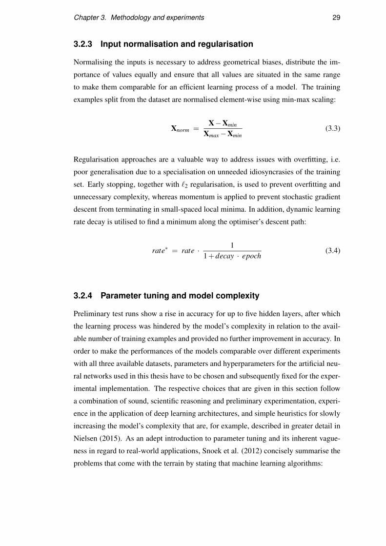
Chapter 3. Methodology and experiments 29
3.2.3 Input normalisation and regularisation
Normalising the inputs is necessary to address geometrical biases, distribute the im-
portance of values equally and ensure that all values are situated in the same range
to make them comparable for an efficient learning process of a model. The training
examples split from the dataset are normalised element-wise using min-max scaling:
Xnorm =X−Xmin
Xmax−Xmin(3.3)
Regularisation approaches are a valuable way to address issues with overfitting, i.e.
poor generalisation due to a specialisation on unneeded idiosyncrasies of the training
set. Early stopping, together with `2 regularisation, is used to prevent overfitting and
unnecessary complexity, whereas momentum is applied to prevent stochastic gradient
descent from terminating in small-spaced local minima. In addition, dynamic learning
rate decay is utilised to find a minimum along the optimiser’s descent path:
rate∗ = rate · 11+decay · epoch
(3.4)
3.2.4 Parameter tuning and model complexity
Preliminary test runs show a rise in accuracy for up to five hidden layers, after which
the learning process was hindered by the model’s complexity in relation to the avail-
able number of training examples and provided no further improvement in accuracy. In
order to make the performances of the models comparable over different experiments
with all three available datasets, parameters and hyperparameters for the artificial neu-
ral networks used in this thesis have to be chosen and subsequently fixed for the exper-
imental implementation. The respective choices that are given in this section follow
a combination of sound, scientific reasoning and preliminary experimentation, experi-
ence in the application of deep learning architectures, and simple heuristics for slowly
increasing the model’s complexity that are, for example, described in greater detail in
Nielsen (2015). As an adept introduction to parameter tuning and its inherent vague-
ness in regard to real-world applications, Snoek et al. (2012) concisely summarise the
problems that come with the terrain by stating that machine learning algorithms:

Chapter 3. Methodology and experiments 30
”[...] frequently require careful tuning of model hyperparameters, regu-larization terms, and optimization parameters. Unfortunately, this tuningis often a ”black art” that requires expert experience, unwritten rules ofthumb, or sometimes brute-force search.” (Snoek et al., 2012)
While such a statement sounds bleak, the parameters and hyperparameters that have to
be set can be determined, or at least approximated: Due to the dependence of a viable
number of neurons for hidden layers on the particular problem that is addressed, this
number is approximated by experiments on a subset of the problem, and 400 nodes per
hidden layer are chosen as a size slightly below the number of inputs for the experi-
ments. Preliminary tests with 20 randomly chosen stocks for each of the three datasets
with half-hour, one-hour and one-day gradients show the smallest test set error for this
size of hidden layers, as measured in increments of 50 nodes for up to 800 nodes. To
address potential memory issues, a mini-batch size of 100 is chosen in order to use
stochastic gradient decent on a randomly selected batch at a time, and each model is
trained for 50 epochs, with early stopping as a regularisation measure as described in
Section 3.2.3. In addition, `2 regularisation is added to the regularisation process and
chosen over `1 regularisation. The reason behind this decision is the encouragement
to use all inputs to a certain degree, as a complex interdependence of the studied time
series is assumed due to the failures of past approaches to identify simpler correlations.
Through this introduction of decaying weights, and with the parameter λ defining the
trade-off between the loss function and the penalty for larger weights, the previously
introduced notation for unaltered gradient descend in Formula (2.7) is extended to:
w j,i = w j,i−η∂E
∂w j,i−ηλw j,i (3.5)
Hyperbolic tangent functions from Formula (2.4) serve as activation functions, with
sigmoid functions from Formula (2.3) at the output layer. The former choice is due to
the reasons regarding weight saturation given in Section 2.2.1, while the latter function
is chosen over the softmax function due to the interpretability of the results as indepen-
dent probabilities, and because these results are not needed to integrate to 1 as inputs
for subsequent methods. The model’s weights are initialised as scaled samples from
a zero-mean Gaussian distribution to address the potential of vanishing or exploding
gradients, with a standard deviation of√
2nl
and an initial bias of 0, and with nl de-
noting the number of connections in a layer, allowing for an easy adaptation to future
experiments with rectified linear units (Glorot and Bengio, 2010; He et al. 2015).

Chapter 3. Methodology and experiments 31
3.3 Further experiments and high volatility
3.3.1 Complexity reduction via bottleneck layers
In the context of the given problem, an interesting question is that of its general com-
plexity, i.e. to find out to what number of variables the relevant data necessary for an
acceptable accuracy can be reduced. In order to give an indication, a bottleneck layer
consisting of a small number of neurons is inserted into the models for the daily pre-
dictions based on the 5-year dataset with hourly values. This process is implemented
for 1, 3, 5 and 10 nodes to see how the bottleneck’s size influences the accuracy. The
results are subsequently presented in Section 4.2.1. This approach is favoured over
using autoencoders as a precedent step before using their compression layer as inputs
for a full model, as autoencoders learn a goalless reduction of their inputs. For a bottle-
neck layer in the same model, the latter is forced to learn a compressed representation
directed at a representation that is suited for the target predictions at hand, funnelling
the model’s learning process through the nodes of the respective bottleneck. Figure
3.2 shows a modification of the model previously depicted in Figure 3.1, featuring an
exemplary additional bottleneck layer for complexity tests with one node marked as b:
Figure 3.2: Model with a one-neuron bottleneck layer

Chapter 3. Methodology and experiments 32
3.3.2 Performance during a financial crisis
As one of the first publications on machine learning for stock market prediction that
gathered considerable news coverage, the AZFinText system devised by Schumaker
and Chen (2009a) notably was not tested for above-average results in selectively volatile
market situations, although the authors note such a test as a suggestion for further re-
search. For time series-based prediction approaches, high-volatility environments are
worse than for text analysis-based systems like AZFinText, as they solely rely on the
stock market information that is in turmoil in such a scenario. To test the gradient-
based approach and the model implementation for such environments, data from 2003
to, and including, 2008 is extracted from the 20-year dataset with hourly values to
compute daily gradients for the contained stock price information and 298 stocks.
No cross-validation is performed for these experiments, as the test set has to repre-
sent a phase of enhanced volatility in the market. In order to reach that goal, a test set
from July 2007 to the end of 2008 is split from the set of gradients, with the previous
4.5 years serving as training data. This setup also more closely resembles an applicable
prediction system, as only past data is used instead of identifying general correlations
between combinations of different time periods through cross-validation. Due to the
large fluctuations in the dataset, and given that some stocks remained more stable than
others during the financial crisis of 2007/2008, a higher variance of accuracies is ex-
pected. An accuracy above the baseline, which is expected to be higher than random
chance due to the general negative trend in that time period, would deliver evidence for
the persistence of correlations in high-volatility scenarios such as global market crises.
3.4 Reliability of the obtained findings
3.4.1 Distinction against coincidences
For a validation of the results, baselines that address the market behaviour and the
distributions of target vectors are necessary in order to find statistically significant ev-
idence. The focus of this thesis on time-shifted correlations between stocks in relation
to economic theory, which is also manifested in leaving out information of the target
stock in the models’ inputs, sets this work apart from research that aims to find the
best-possible stock market predictions instead of correlations in stock market prices.

Chapter 3. Methodology and experiments 33
For research focussed purely on prediction accuracy, baselines that represent naıve
regression or classification approaches, or more basic machine learning methods, are
more suitable and also used in the research discussed in Section 2.1.3. The threat
of coincidences is partly approached through cross-validation, but a model’s accuracy
must also lie significantly above the accuracies of one-value and random predictions.
3.4.2 Accuracy of random mock predictions
For each stock and fold in each model, a randomly shuffled copy of the predictions is
created and tested against the correct targets in addition to the predictions themselves,
resulting in mock predictions with a class distribution identical to the actual predic-
tions. This copy can be used to test whether the model just learned the distribution of
the two output classes in the training set, which would result in very similar accuracies
for the actual and mock predictions when compared to the test set’s correct targets.
3.4.3 Tests for one-sided distribution learning
Another case that has to be ruled out is that of a model learning to predict the dom-
inant class of the respective training set. In order to address this potential issue, two
targets are created for each stock and model, each containing exclusively one of the
two classes. A model that learns more actionable information from its respective in-
puts than the dominant class of the training set needs to perform better on the test set
than both these one-class mock targets in direct comparison to the correct targets.
3.4.4 Statistical validation metrics
The average accuracies for each model over all stocks are given as the standard method
to assess the predictive power of a model. These accuracies do not, however, give
an indication as to whether the predictions’ variations are too large to be considered
successful in the context of this thesis. For this reason, the accuracies for the three
baseline mock predictions are also given, as well as the lower bound of a confidence
interval. In addition, the p-values for the predictions’ accuracies via an upper-tail test
are calculated for each of the three baselines and an additional baseline that contains
the highest accuracy among the three baselines for each stock, i.e. for each model. The
null hypothesis H0 in each case is that the predictions’ accuracies are not significantly
larger than the respective baseline, with a very strict significance level of α = 0.001.

Chapter 4
Experimental results
After the introduction in Chapter 1, Chapters 2 and 3 covered the background research
that was conducted in the course of this thesis, as well as the methodology for the
experiments and the validation procedures. This chapter summarises the results of
the experiments and the related values for the statistical key performance indices as
the basis for the subsequent discussion of the findings in Chapter 5, providing both
graphical representations of the results as an overview and tables of the specific values.
4.1 Results of the primary experiments
Notched box-and-whisker plots are a commonly used visualisation tool for descrip-
tive statistics, using the respective data’s quartiles to allow for an intuitive representa-
tion. The lower and upper ends of a box indicate the first and third quartile, while the
median is depicted as a horizontal bar. The whiskers show the lowest and highest data
point that is within 1.5-times the interquartile range of the first and third quartile:
whiskerupper = min(max(data), Q3 +1.5 · (Q1−Q3)) (4.1)
whiskerlower = max(min(data), Q1−1.5 · (Q1−Q3)) (4.2)
Outliers are shown above or below the whiskers, and non-overlapping notches for two
boxes indicate a statistically significant median difference at 95% confidence. Welch’s
t-test is used to achieve a higher reliability for unequal variances. For every experi-
ment, the accuracies for the model and the baselines are given, as well as the p-value
results w.r.t. the means and the minimal difference for a 99.9% confidence interval. In
Table 4.1 and subsequent tables, class 1 is the prediction that stock trends will change
downwards, and class 2 is the prediction that stock trends will change upwards.
34

Chapter 4. Experimental results 35
4.1.1 One-day gradient intervals
Figure 4.1: Box plots for accuracies for one-day time intervals
Figure 4.1 shows that the accuracy of 56.02% listed in Table 4.1 lies significantly above
all baselines, both for the means as measured by the p-values and the medians as indi-
cated by the box plots, with neither the notches nor the boxes themselves overlapping.
The first and third quartiles are, however, spread wider for the accuracy of the model.
accuracies of predictions
model randomised class 1 class 2 best-of
~ 0.5602 ~ 0.5002 ~ 0.4955 ~ 0.5045 ~ 0.5092
tests against baselines
randomised class 1 class 2 best-of
p-value p < 0.001 p < 0.001 p < 0.001 p < 0.001
min. diff. ~ 0.0559 ~ 0.0607 ~ 0.0518 ~ 0.0471
Table 4.1: Statistical KPIs for one-day intervals

Chapter 4. Experimental results 36
4.1.2 One-hour gradient intervals
Figure 4.2: Box plots for accuracies for one-hour time intervals
With an accuracy of 53.95%, the model’s accuracies exhibit the same increased vari-
ability as for one-day gradients, albeit with a smaller spread. The baselines’ accuracies
are centred more closely on 50%, which is consistent with the overall smaller spread of
the accuracies for both the model and the baselines, trading accuracy for narrowness.
accuracies of predictions
model randomised class 1 class 2 best-of
~ 0.5395 ~ 0.5008 ~ 0.4973 ~ 0.5027 ~ 0.5043
tests against baselines
randomised class 1 class 2 best-of
p-value p < 0.001 p < 0.001 p < 0.001 p < 0.001
min. diff. ~ 0.0356 ~ 0.0392 ~ 0.0338 ~ 0.0322
Table 4.2: Statistical KPIs for one-hour intervals

Chapter 4. Experimental results 37
4.1.3 Half-an-hour gradient intervals
Figure 4.3: Box plots for accuracies for half-an-hour time intervals
For a model accuracy of 51.70%, the trend to lower model accuracies in relation to
the gradients’ time frame, together with narrower boxes for the baselines depicting the
quartile ranges of the accuracy values, persists. The distribution of the model’s accu-
racies also are skewed towards lower values, i.e. more variability above the median.
accuracies of predictions
model randomised class 1 class 2 best-of
~ 0.5170 ~ 0.5011 ~ 0.4979 ~ 0.5021 ~ 0.5030
tests against baselines
randomised class 1 class 2 best-of
p-value p < 0.001 p < 0.001 p < 0.001 p < 0.001
min. diff. ~ 0.0137 ~ 0.0169 ~ 0.0127 ~ 0.0118
Table 4.3: Statistical KPIs for half-an-hour intervals

Chapter 4. Experimental results 38
4.2 Complexity and volatile environments
4.2.1 Results for models with bottlenecks
Figure 4.4: Box plots for accuracies for different bottleneck sizes
To show the effect of bottlenecks sizes as described in Section 3.3.1, the box plots for
four cases are depicted in Figure 4.4. The models’ accuracies, as shown in Table 4.4,
are significantly increasing with the steps taken for the number of nodes used in the
respective bottlenecks, with 10 bottleneck nodes resulting in an accuracy slightly below
the full model without a bottleneck. The quartile ranges of the box plots, remaining
approximately symmetrical, also increase with a higher number of bottleneck nodes.
accuracies of predictions
1 node 3 nodes 5 nodes 10 nodes no bottleneck
~ 0.5107 ~ 0.5309 ~ 0.5395 ~ 0.5503 ~ 0.5602
Table 4.4: Statistical KPIs for bottleneck models

Chapter 4. Experimental results 39
4.2.2 Robustness in a crisis scenario
Figure 4.5: Box plots for accuracies for high-volatility environments
The range of depicted accuracies has to be changed to accommodate all values, as a
high accuracy of 61.13% is accompanied by a large spread and imbalanced target dis-
tributions. Notably, the medians and mean accuracies for one-class predictions show
that the price trends more often changed downwards during this volatile scenario.
accuracies of predictions
model randomised class 1 class 2 best-of
~ 0.6113 ~ 0.5301 ~ 0.4405 ~ 0.5595 ~ 0.5607
tests against baselines
randomised class 1 class 2 best-of
p-value p < 0.001 p < 0.001 p < 0.001 p < 0.001
min. diff. ~ 0.0677 ~ 0.1589 ~ 0.0399 ~ 0.0388
Table 4.5: Statistical KPIs for high-volatility environments

Chapter 5
Discussion
After the introduction and background research of Chapters 1 and 2, and following the
explanation of the methodology and the presentation of the results in Chapters 3 and 4,
this chapter contains a discussion of the findings. The results and their validity, includ-
ing the experiments for complexity and high-volatility environments, are investigated
in the context of comparable research and considerations regarding the implications of
the problem’s complexity, as well as the broader framework of the economic theory
that is involved in the presented application to real-world stock market information.
5.1 Findings of the primary experiments
5.1.1 Analysis and validation of the findings
The usage of p-values for validation purposes has to be viewed with caution, as crit-
icism of their abundant and often incorrect use has risen in recent years. In 2016,
the American Statistical Association published an official warning regarding the wide-
spread misuse of p-values (Wasserstein and Lazar, 2016). Accordingly, the p-values
in Chapter 4 are given in combination with other metrics such as the lower boundary
for differences in means given a 99.9% confidence interval, notched box-and-whisker
plots for median differences and quartile distributions, and accuracies for both the mod-
els and the separate baselines. In combination, these metrics deliver strong evidence
for the economic part of the investigated hypothesis, i.e. that price series in historical
stock market data contain time-shifted correlations that can be successfully exploited
with deep-layered feedforward neural networks, resulting in above-baseline price trend
predictions without data of the target stock present in the inputs of the models.
40

Chapter 5. Discussion 41
Notably, larger time intervals for gradient calculations and predictions based on the
latter result in higher average accuracies, but with a trade-off in the form of an in-
creased spread of the accuracies, i.e. a larger variance. Given the described confidence
interval, this leads to the lower bounds for one-day predictions and for half-an-hour
predictions in relation to their true difference in means differing by 7.10% in favour of
one-day predictions. It therefore seems to be easier for the models to learn correlations
between gradients and make corresponding predictions for larger time steps. A natu-
ral explanation for these differences is the presence of more noise in short-time stock
observations, indicating that noise is smoothed out for regressions over larger intervals.
Similarly, the part of the hypothesis dealing with general time series analysis via such
network models is reinforced: The evidence strongly suggests that deep-layered feed-
forward neural networks can be used to consistently learn and, for previously unseen
data, act with an accuracy above predetermined baselines on time-shifted correlations
of gradients that are computed step-wise for complex time series, with only the pre-
vious interval as input features. The approach of this thesis could be applied to other
kinds of forecasting problems that involve non-linear interactions between a large num-
ber of time series and lagged effects of their trend behaviour, e.g. the metrics in areas
as diverse as consumer behaviour and epidemic dynamics for infectious diseases.
5.1.2 Comparison with related research
While meta-analyses should always be interpreted cautiously due to the possibility of
publication biases, Park and Irwin (2004) find that a majority of published research
dealing with technical analysis for stock market prediction reports results that indicate
a problem for the efficient-market hypothesis in its strict form. As research on deep
learning for time series-based stock market prediction is still sparse, there are two
research results that can be used to compare this thesis: Both Takeuchi and Lee (2013)
and Batres-Estrada (2015) use deep-layered neural network models for a binary month-
wise trend prediction of target stocks, based on historical stock market data of the
preceding 12 months, with resulting accuracies of 53.36% and 52.89% respectively. A
direct comparison is still an approximation, as this thesis addresses the prediction of
up- and downward changes in the trend gradient instead of the target gradient’s sign,
but the binary prediction of either targets is comparable in their perceived difficulty
and exclusion by the efficient-market hypothesis and the random walk hypothesis.

Chapter 5. Discussion 42
An additional difference is the time frame that is used for predictions, as this thesis is
validated by one-day, one-hour and half-an-hour predictions instead of full months, as
well as the richness of the training inputs, for which this thesis uses only the price gra-
dients, and only for the time interval directly preceding the prediction target. Despite
the more limited features, the accuracies for one-day and one-hour predictions surpass
both Takeuchi and Lee (2013) and Batres-Estrada (2015), with 56.02% and 53.95%.
The approach of this thesis also proved to be capable of extracting additional infor-
mation in high-volatility scenarios with imbalanced trend targets, albeit with a higher
variance of the accuracies than in non-volatile market environments. Notably, one of
the findings is that accuracies decrease with smaller time intervals, which would make
a comparison with one-day intervals for the two comparable publications an interest-
ing research topic, increasing the comparability of these different approaches.
In summary, the approach taken for the development of this thesis outperforms both
examples of binary trend prediction using past stock market time series, without the
utilisation of information about the target stock itself, as the goal was to show time-
shifted correlations of stock prices. It can therefore be inferred that the presented
research could potentially be applied to profitable stock trading, although prediction
accuracies are only the success metric used for the testing of economic theory in the
context of this thesis, making such a usage a practical application of the results. In
such a case, it is recommended to include information of the target stock in the inputs.
5.1.3 Discussion of possible shortfalls
During the cleansing and pre-processing of the datasets, missing observations for
stocks, the absence of which is not consistent for all stocks represented in the dataset,
are approximated by the next time-wise adjacent intact observation for the same stock,
as described in Section 3.1.3 and using the algorithm in Appendix A. This approx-
imation process, although not resulting in a comparably large amount of insertions,
represents a marginal distortion of the data and could influence the results. As histor-
ical stock market data is often faulty, even for the professional data provider used for
this thesis, this is a necessary evil, but it should be mentioned here. In addition, the
datasets cover only the S&P 500 stocks, and it remains an interesting research ques-
tion whether the inclusion of less prominent stocks further boosts the models’ perfor-
mances, or whether the same time-shifted correlations exist in other sets of stocks.
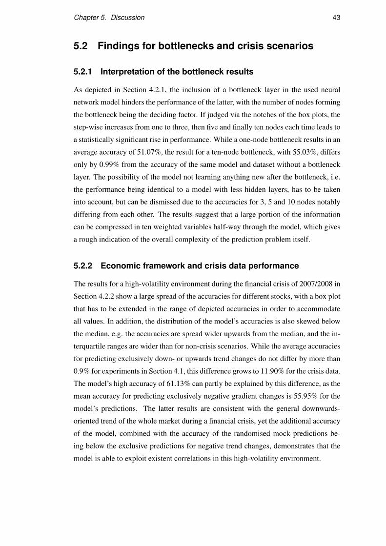
Chapter 5. Discussion 43
5.2 Findings for bottlenecks and crisis scenarios
5.2.1 Interpretation of the bottleneck results
As depicted in Section 4.2.1, the inclusion of a bottleneck layer in the used neural
network model hinders the performance of the latter, with the number of nodes forming
the bottleneck being the deciding factor. If judged via the notches of the box plots, the
step-wise increases from one to three, then five and finally ten nodes each time leads to
a statistically significant rise in performance. While a one-node bottleneck results in an
average accuracy of 51.07%, the result for a ten-node bottleneck, with 55.03%, differs
only by 0.99% from the accuracy of the same model and dataset without a bottleneck
layer. The possibility of the model not learning anything new after the bottleneck, i.e.
the performance being identical to a model with less hidden layers, has to be taken
into account, but can be dismissed due to the accuracies for 3, 5 and 10 nodes notably
differing from each other. The results suggest that a large portion of the information
can be compressed in ten weighted variables half-way through the model, which gives
a rough indication of the overall complexity of the prediction problem itself.
5.2.2 Economic framework and crisis data performance
The results for a high-volatility environment during the financial crisis of 2007/2008 in
Section 4.2.2 show a large spread of the accuracies for different stocks, with a box plot
that has to be extended in the range of depicted accuracies in order to accommodate
all values. In addition, the distribution of the model’s accuracies is also skewed below
the median, e.g. the accuracies are spread wider upwards from the median, and the in-
terquartile ranges are wider than for non-crisis scenarios. While the average accuracies
for predicting exclusively down- or upwards trend changes do not differ by more than
0.9% for experiments in Section 4.1, this difference grows to 11.90% for the crisis data.
The model’s high accuracy of 61.13% can partly be explained by this difference, as the
mean accuracy for predicting exclusively negative gradient changes is 55.95% for the
model’s predictions. The latter results are consistent with the general downwards-
oriented trend of the whole market during a financial crisis, yet the additional accuracy
of the model, combined with the accuracy of the randomised mock predictions be-
ing below the exclusive predictions for negative trend changes, demonstrates that the
model is able to exploit existent correlations in this high-volatility environment.

Chapter 6
Conclusion
Chapters 1 to 5 introduce, describe and discuss the hypothesis, background research
and experimental evidence gathered during the course of this project. As the final part
of this thesis, this chapter concludes the presented research by summarising the im-
plications of the findings and the contributions to the involved fields of research. In
addition, suggestions for further research are given to inspire future investigative en-
deavours at the intersection of deep learning, economic theory and time series analysis.
6.1 Summary of the findings
The findings of the presented research deliver evidence for time-shifted correlations
between the price behaviour of S&P 500 stocks in contradiction to both the random
walk hypothesis and the efficient-market hypothesis in all three forms, and for the vi-
ability of using deep-layered neural networks for trend prediction in intercorrelated
time series. The hypothesis described in Section 1.3. is, within the margins of empir-
ical evidence and its statistical validation, confirmed and outperforms the predefined
baselines for strict statistical key performance indices and within all performed experi-
ments. Predictions of one stock’s trend changes based on other stock’s price trend gra-
dients in the preceding time step show an improved accuracy for larger time intervals,
with average accuracies and maximum accuracies of 56.02% and 63.95% respectively
for one-day predictions. They retain large parts of their accuracy for a minimum of 10
nodes for mid-model bottleneck layers, and show equally above-baseline predictions in
high-volatility market scenarios, albeit with the cost of a higher variance for different
stocks. In conclusion, the results of this thesis in regard to the investigated hypothesis
are positive under conscientious observance of statistical validation measures.
44

Chapter 6. Conclusion 45
6.2 Contributions to existing theory
This thesis delivers strong evidence against the random walk hypothesis and the efficient-
market hypothesis. The postulates of the latter can, however, be adapted to allow
for these findings: While all forms of the efficient-market hypothesis contradict the
presented evidence due to the prohibition of successful technical analysis, a possible
change to the weak-form efficient market hypothesis’ postulates is to include prediction
methods that are able to reliably outperform the market and implemented by a suffi-
ciently small number of investors to not result in a new equilibrium. With a negligible
amount of capital involved in the context of the whole market, some agents, e.g. select
quantitative hedge funds or individuals, could consistently realise above-average re-
turns, reducing the weak-form efficient-market hypothesis to a context-based version.
A time-specific weak-form efficient-market hypothesis would state that the postulates
do not apply for general market dynamics, but are true for the majority of the trad-
ing entities due to restrictions regarding the methodology and the capital involved in
the latter. Stock markets would therefore not be seen as inherently efficient, but as
efficient for the majority in the current state of the market. Due to the dismissal of
inherent informational efficiency, the large-scale availability of such methods would
not reinstate the current forms of the efficient-market hypothesis via an equilibrium, as
they categorically prohibit the viability of technical analysis. In addition, the results for
volatile environments, by using pre-crisis data to for the training process, contributes
some evidence for the Dragon King Theory of Sornette (2009) and the research de-
scribed in Section 2.1.2. The large difference in accuracies for the model’s predictions
and the baselines can not be explained by the shift to a skewed distribution in favour of
negative trend changes, given that the training data does not contain such an imbalance.
In regard to the application of deep learning to time series analysis, the results pre-
sented in this thesis deliver evidence for the viability of deep-layered neural networks
and gradient features for trend change prediction with non-linear correlations of a large
number of time series, with possible areas of application proposed in Section 5.1.1. As
discussed in Section 1.4.3, the positive results of this thesis demonstrate the value of
deep learning approaches to time series analysis and show the utility of linear regres-
sion derivatives as features, offering a simple trend indicator with a high predictive
value in order to further the understanding of highly complex time series correlations.

Chapter 6. Conclusion 46
6.3 Suggestions for further research
6.3.1 Investigation of high frequency data
High frequency trading refers to the utilisation of high frequency market data with
short holding periods and high cancellation rates for automated equities and futures
trading (Menkveld, 2013). Although its share of all implemented trades decreased after
the financial crisis of 2007/2008, high frequency trading remains a driving force on
financial markets, with a double-digit share of total trading volumes across markets and
competition existing mostly between different algorithms (Easley et al., 2010). With
the presented model structure, the presence of small-scale time-shifted correlations
could be detected to investigate the interdependence of high frequency trading systems.
6.3.2 Integration of text-based approaches
As described in Section 2.1.4, research on text analysis-based stock market prediction
has been shown to be capable of profitable returns. The combination with time series-
based predictions has been tested before, with indications that such a combination of
information gathered from both finance-related textual news and historical stock mar-
ket data is viable (Cao et al., 2012). Given that the analysis of news feeds constitutes
new information, related experiments could not be used to test market efficiency and
would be a practical application of this thesis for optimised stock market prediction.
6.3.3 Wavelets as advanced features
Wavelets are the result of time-frequency transformations to obtain a representation of
local variations on different scales. An example of a comprehensive introduction to
their usage for time series analysis is Nason and von Sachs (1999). Section 2.3.3 gives
an overview of gradient-based wavelet approaches to practical applications in regard to
time series, and it is proposed that wavelets could be used as a more sophisticated way
to extract relevant information from time intervals of stock price series. As wavelets are
useful for denoising signals, the research question in this case would be whether this
elaborate form of information extraction yields better model performances for stock
price predictions than trend approximations via linear regressions over time intervals.

Appendix A
Main function for the substitution of missing instances:
# F u n c t i o n t o a c c o u n t f o r m i s s i n g t ime s tamps
m i s s i n g i n s t a n c e s <− f u n c t i o n ( da t a , s t o c k s . num , v a l i d . t imes , ) {d a t a . l i s t <− l i s t ( ) ;
f o r ( i i n 1 : s t o c k s . num ) {d a t a . l i s t [ [ i ] ] <− d a t a [ ( data$X . RIC == un iq ue . r i c [ i ] ) , ] ;
}c o u n t . l i s t <− l i s t ( ) ;
f o r ( i i n 1 : s t o c k s . num ) {c o u n t . l i s t [ [ i ] ] <− d a t a . l i s t [ [ i ] ] $Time . L . [ 1 ] ;
}c o u n t . wrong <− u n l i s t ( c o u n t . l i s t ) ;
c o u n t . wrong <− which ( c o u n t . wrong != v a l i d . t i m e s [ 1 ] ) ;
f o r ( i i n c o u n t . wrong ) {d a t a . s t a r t <−
as . i n t e g e r ( s u b s t r i n g ( d a t a . l i s t [ [ i ] ] $Time . L . [ 1 ] , 1 , 2 ) ) ;
v a l i d . s t a r t <− as . i n t e g e r ( s u b s t r i n g ( v a l i d . t i m e s [ 1 ] , 1 , 2 ) ) ;
s t a r t . d i f f <− d a t a . s t a r t − v a l i d . s t a r t ;
d a t a . l i s t [ [ i ] ] [ ( 1 + s t a r t . d i f f ) : ( dim ( d a t a . l i s t [ [ i ] ] ) [ 1 ]
+ s t a r t . d i f f ) , ]
<− d a t a . l i s t [ [ i ] ] [ 1 : dim ( d a t a . l i s t [ [ i ] ] ) [ 1 ] , ] ;
f o r ( j i n 1 : s t a r t . d i f f ) {d a t a . l i s t [ [ i ] ] [ j , ] <− d a t a . l i s t [ [ i ] ] [ ( 1 + s t a r t . d i f f ) , ]
d a t a . l i s t [ [ i ] ] $Time . L . [ j ] <− v a l i d . t i m e s [ j ] ;
}}f o r ( i i n 1 : s t o c k s . num ) {
d a t a . l i s t [ [ i ] ] <− f i l l i n s t a n c e s ( d a t a . l i s t [ [ i ] ] , v a l i d . t i m e s ) ;
d a t a . l i s t [ [ i ] ] <− na . omi t ( d a t a . l i s t [ [ i ] ] ) ;
}r e t u r n ( d a t a . l i s t ) ;
}
x

xi
Auxiliary function for missinginstances():
# F u n c t i o n t o d e t e c t and f i l l m i s s i n g i n s t a n c e s
f i l l i n s t a n c e s <− f u n c t i o n ( da t a , v a l i d . t i m e s ) {r u l e r <− dim ( d a t a ) [ 1 ] ;
i n p u t . l e n g t h <− r u l e r ;
d a t a <− r b i n d ( da t a , d a t a ) ;
d a t a . l e n g t h <− dim ( d a t a ) [ 1 ] ;
da ta$Type [ ( i n p u t . l e n g t h + 1 ) : d a t a . l e n g t h ] <− NA;
t i m e s <− da ta$Time . L . ;
t i m e s . new <− r e p ( v a l i d . t imes , l e n g t h . o u t = i n p u t . l e n g t h ) ;
i d . t i m e s <− FALSE ;
w h i l e ( ! ( i d . t i m e s == TRUE ) ) {l o c . d i f f <− min ( which ( ( t i m e s == t i m e s . new ) == FALSE ) ) ;
i f ( ( l o c . d i f f == I n f ) | | i s . na ( da ta$Type [ l o c . d i f f ] ) ) {i d . t i m e s <− TRUE;
} e l s e {d a t a [ ( l o c . d i f f + 1 ) : ( r u l e r + 1 ) , ] <− d a t a [ l o c . d i f f : r u l e r , ] ;
ho ld . t ime <− t i m e s . new [ l o c . d i f f ] ;
i f ( data$X . RIC [ l o c . d i f f ] == data$X . RIC [ l o c . d i f f − 1 ] ) {d a t a [ l o c . d i f f , ] <− d a t a [ l o c . d i f f − 1 , ] ;
} e l s e {d a t a [ l o c . d i f f , ] <− d a t a [ l o c . d i f f + 1 , ] ;
}da ta$Time . L . [ l o c . d i f f ] <− ho ld . t ime ;
r u l e r <− r u l e r + 1 ;
t i m e s <− da ta$Time . L . ;
}}d a t a <− d a t a [ 1 : ( min ( which ( i s . na ( da ta$Type ) ) ) − 1 ) , ] ;
d a t a <− d a t a [ , ! ( names ( d a t a ) %i n% ’ Type ’ ) ] ;
r e t u r n ( d a t a ) ;
}
Input explanation:
data is a matrix without NA values containing a dataset with a structure as described
in Section 3.1.2. stocks.num is the number of unique stocks represented in data, and
valid.times is a vector of valid successive time stamps of the same length as the
number of rows in data. The output of missinginstances() is a list with one list
place for each unique stock in data that contain matrices that can be aligned perfectly.

Appendix B
Reuters Instrument Codes for the primary and bottleneck experiments:
AA.N AAPL.OQ AAP.N ABC.N ABT.N ACN.N ADBE.OQ
ADM.N ADP.OQ ADSK.OQ ADS.N AEE.N AEP.N AES.N
AET.N AFL.N AIG.N AIV.N AIZ.N AKAM.OQ ALL.N
ALXN.OQ AMAT.OQ AME.N AMG.N AMGN.OQ AMP.N AMT.N
AMZN.OQ A.N AN.N AON.N APA.N APC.N APD.N
APH.N ARG.N ATVI.OQ AVB.N AVGO.OQ AVY.N AWK.N
AXP.N AZO.N BAC.N BA.N BAX.N BBBY.OQ BBT.N
BBY.N BCR.N BDX.N BEN.N BFb.N BHI.N BIIB.OQ
BK.N BLK.N BLL.N BMY.N BRKb.N BSX.N BWA.N
BXP.N CAG.N CAH.N CA.OQ CAT.N CBG.N CB.N
CBS.N CCE.N CCI.N CCL.N CELG.OQ CERN.OQ CF.N
CHD.N CHK.N CHRW.OQ CI.N CINF.OQ CL.N CLX.N
CMA.N CMCSA.OQ CME.OQ CMG.N CMI.N CMS.N C.N
CNC.N CNP.N COF.N COG.N COH.N COL.N COP.N
COST.OQ CPB.N CRM.N CSCO.OQ CTAS.OQ CTL.N CTSH.OQ
CTXS.OQ CVC.N CVS.N CVX.N CXO.N DAL.N DD.N
DE.N DFS.N DG.N DGX.N DHI.N DHR.N DISCA.OQ
DISCK.OQ DIS.N DLTR.OQ D.N DNB.N DO.N DOV.N
DOW.N DPS.N DRI.N DTE.N DUK.N DVA.N DVN.N
EBAY.OQ ECL.N ED.N EFX.N EIX.N EL.N EMC.N
EMN.N EMR.N ENDP.OQ EOG.N EQIX.OQ EQR.N EQT.N
ESRX.OQ ESS.N ETFC.OQ ETN.N ETR.N EW.N EXC.N
EXPD.OQ EXPE.OQ EXR.N FAST.OQ FCX.N FDX.N FE.N
FFIV.OQ FIS.N FISV.OQ FITB.OQ FLIR.OQ FL.N FLR.N
FLS.N FMC.N F.N FRT.N FSLR.OQ FTI.N GD.N
GE.N GGP.N GILD.OQ GIS.N GLW.N GME.N GM.N
GOOG.OQ GPC.N GPN.N GPS.N GRMN.OQ GS.N GWW.N
HAL.N HAR.N HAS.OQ HBAN.OQ HBI.N HCA.N HCN.N
xii

xiii
HCP.N HD.N HES.N HIG.N HOG.N HOLX.OQ HON.N
HOT.N HP.N HPQ.N HRB.N HRL.N HRS.N HSIC.OQ
HST.N HSY.N HUM.N IBM.N ICE.N IFF.N ILMN.OQ
INTC.OQ INTU.OQ IPG.N IP.N IRM.N IR.N ISRG.OQ
ITW.N IVZ.N JBHT.OQ JCI.N JEC.N JNJ.N JNPR.N
JPM.N JWN.N KEY.N KIM.N KLAC.OQ KMB.N KMI.N
KMX.N K.N KO.N KR.N KSS.N KSU.N LEG.N
LEN.N LH.N LLL.N LLTC.OQ LLY.N LM.N LMT.N
L.N LNC.N LOW.N LRCX.OQ LUK.N LUV.N LYB.N
MAC.N MA.N MAS.N MAT.OQ MCD.N MCHP.OQ MCK.N
MCO.N MDT.N MET.N MHK.N MJN.N MKC.N MLM.N
MMC.N MMM.N M.N MO.N MON.N MOS.N MRK.N
MRO.N MSFT.OQ MSI.N MS.N MTB.N MU.OQ MUR.N
MYL.OQ NBL.N NDAQ.OQ NEE.N NEM.N NFLX.OQ NFX.N
NI.N NKE.N NLSN.N NOC.N NOV.N NRG.N NSC.N
NTAP.OQ NTRS.OQ NUE.N NVDA.OQ NWL.N NWSA.OQ NWS.OQ
OI.N OKE.N OMC.N O.N ORLY.OQ OXY.N PAYX.OQ
PBCT.OQ PBI.N PCAR.OQ PCG.N PCLN.OQ PDCO.OQ PEG.N
PEP.N PFE.N PFG.N PG.N PHM.N PH.N PKI.N
PLD.N PM.N PNC.N PNR.N PNW.N PPG.N PPL.N
PRU.N PSA.N PVH.N PWR.N PXD.N PX.N QCOM.OQ
RAI.N RCL.N RF.N RHI.N RHT.N RIG.N RL.N
R.N ROK.N ROP.N ROST.OQ RRC.N RSG.N RTN.N
SBUX.OQ SCG.N SCHW.N SEE.N SE.N SHW.N SIG.N
SJM.N SLB.N SLG.N SNA.N SNDK.OQ SO.N SPG.N
SPLS.OQ SRCL.OQ SRE.N STI.N STJ.N STT.N STX.OQ
STZ.N SWK.N SWKS.OQ SWN.N SYK.N SYMC.OQ SYY.N
TAP.N TDC.N TEL.N TE.N TGT.N TIF.N TJX.N
TMK.N TMO.N T.N TROW.OQ TRV.N TSCO.OQ TSN.N
TSO.N TSS.N TWC.N TWX.N TXT.N TYC.N UAL.N
UA.N UDR.N UHS.N ULTA.OQ UNH.N UNM.N UNP.N
UPS.N URBN.OQ URI.N USB.N UTX.N VAR.N VFC.N
VLO.N VMC.N V.N VNO.N VRSK.OQ VRSN.OQ VRTX.OQ
VTR.N VZ.N WAT.N WEC.N WFC.N WHR.N WMB.N
WM.N WMT.N WU.N WY.N WYN.N WYNN.OQ XEC.N
XEL.N XL.N XOM.N XRAY.OQ XRX.N YHOO.OQ YUM.N
ZION.OQ

xiv
Reuters Instrument Codes for the high-volatility experiments:
AA.N AAP.N ABC.N ABT.N ACN.N ADM.N ADS.N
AEE.N AEP.N AES.N AET.N AFL.N AGN.N AIG.N
AIV.N ALL.N AME.N AMG.N AMT.N A.N AN.N
APA.N APC.N APD.N APH.N ARG.N AVB.N AVY.N
AXP.N AZO.N BAC.N BA.N BAX.N BBT.N BBY.N
BCR.N BDX.N BEN.N BFb.N BHI.N BK.N BLK.N
BLL.N BMY.N BRKb.N BSX.N BWA.N BXP.N CAG.N
CAH.N CAT.N CB.N CCE.N CCI.N CCL.N CHD.N
CHK.N CI.N CL.N CLX.N CMA.N CMS.N C.N
CNP.N COF.N COG.N COH.N COL.N COP.N CPB.N
CTL.N CVC.N CVS.N CVX.N DD.N DE.N DGX.N
DHI.N DHR.N DIS.N D.N DNB.N DO.N DOV.N
DOW.N DRI.N DTE.N DUK.N DVA.N ECL.N ED.N
EFX.N EIX.N EL.N EMC.N EMN.N EMR.N EOG.N
EQR.N EQT.N ESS.N ETN.N ETR.N EW.N EXC.N
FCX.N FDX.N FE.N FLR.N FLS.N FMC.N F.N
FRT.N FTI.N GAS.N GD.N GE.N GIS.N GLW.N
GME.N GM.N GPC.N GPN.N GPS.N GS.N GWW.N
HAL.N HAR.N HCN.N HCP.N HD.N HIG.N HON.N
HOT.N HP.N HPQ.N HRB.N HRL.N HRS.N HSY.N
HUM.N IBM.N IFF.N IPG.N IP.N IRM.N IR.N
ITW.N JCI.N JEC.N JNJ.N JPM.N JWN.N KEY.N
KIM.N KMB.N KMX.N K.N KO.N KR.N KSS.N
KSU.N LEG.N LEN.N LH.N LLL.N LLY.N LM.N
LMT.N LNC.N LOW.N LUK.N LUV.N MAC.N MAS.N
MCD.N MCK.N MCO.N MDT.N MET.N MHK.N MKC.N
MLM.N MMC.N MMM.N MO.N MON.N MRK.N MRO.N
MTB.N MUR.N NBL.N NEM.N NFX.N NI.N NKE.N
NOC.N NSC.N NUE.N NWL.N OI.N OKE.N OMC.N
O.N OXY.N PBI.N PCG.N PEG.N PEP.N PFE.N
PFG.N PG.N PGR.N PHM.N PH.N PKI.N PLD.N
PNC.N PNR.N PNW.N PPG.N PPL.N PRU.N PSA.N
PVH.N PWR.N PXD.N PX.N RCL.N RF.N RHI.N
RIG.N RL.N R.N ROK.N ROP.N RRC.N RSG.N
RTN.N SCG.N SEE.N SHW.N SJM.N SLB.N SLG.N
SNA.N SO.N SPG.N SRE.N STI.N STJ.N STT.N

xv
STZ.N SWK.N SWN.N SYK.N SYY.N TE.N TGT.N
TIF.N TJX.N TMK.N TMO.N T.N TSN.N TSO.N
TSS.N TXT.N TYC.N UDR.N UHS.N UNH.N UNM.N
UNP.N UPS.N URI.N USB.N UTX.N VAR.N VFC.N
VLO.N VMC.N VNO.N VTR.N VZ.N WAT.N WEC.N
WFC.N WHR.N WMB.N WMT.N WY.N XEC.N XEL.N
XL.N XOM.N XRX.N YUM.N

Bibliography
Baggenstoss, P. M. (2015), ”Derivative-augmented features as a dynamic model fortime-series”, Proceedings of the 23rd European Signal Processing Conference(EUSIPCO 2015), pp. 958-962, Naval Undersea Warfare Center (USA), Fraun-hofer FKIE (Germany)
Bahrampour, S.; Ramakrishnan, N.; Schott, L.; Shah, M. (2015), ”Comparative studyof deep learning software frameworks”, working paper, Research and TechnologyCenter, Robert Bosch LLC (USA)
Batres-Estrada (2015), ”Deep learning for multivariate financial time series”, Master’sthesis, KTH Royal Institute of Technology (Sweden)
Barunik, J.; Kukacka, J. (2015), ”Realizing stock market crashes: Stochastic cuspcatastrophe model of returns under time-varying volatility”, Quantitative Finance,Vol. 15, No. 6, pp. 959-973, Charles University in Prague (Czech Republic)
Bergstra, J.; Bastien, F.; Breuleux, O.; Lamblin, P.; Pascanu, R.; Delalleau, O.; Des-jardins, G.; Warde-Farley, D.; Goodfellow, I.; Bergeron, A.; Bengio, Y. (2011),”Theano: Deep learning on GPUs with Python”, Journal of Machine Learning Re-search, Vol. 1, No. 1, pp. 1-48, University of Montreal (Canada)
Berndt, D. J.; Clifford, J. (1994), ”Using dynamic time warping to find patterns in timeseries”, AAAI Workshop on Knowledge Discovery in Databases, pp. 229-248, NewYork University (USA)
Bicchetti, D.; Maystre, N. (2013), ”The synchronized and long-lasting structural changeon commodity markets: Evidence from high frequency data”, Algorithmic Finance,Vol. 2, No. 3-4, pp. 233-239, University of Geneva (Switzerland), United NationsConference on Trade and Development (Switzerland)
xvi

xvii
Bishop. C. (2006), ”Pattern recognition and machine learning”, New York: Springer-Verlag New York, University of Edinburgh (UK)
Broomhead, D.s.; Lowe, D. (1988), ”Multivariable functional interpolation and adap-tive networks”, Complex Systems, Vol. 2, No. 1, pp. 321-355, Royal Signals andRadar Establishment (UK)
Cao, R.; Liang, X.; Ni, Z. (2012), ”Stock price forecasting with support vector ma-chines based on web financial information sentiment analysis”, Lecture Notes inComputer Science: Advanced Data Mining and Applications, Vol. 7713, pp. 527-538, Renmin University of China (PRC)
Chen, N.; Roll, R.; Ross, S. A. (1986), ”Economic forces and the stock market”, TheJournal of Business, Vol. 59, No. 3, pp. 383-403, University of Chicago (USA),University of California, Los Angeles (USA), Yale University (USA)
Chollet, F. (2015), ”Keras”, GitHub, available at: https://github.com/fchollet/keras (ac-cessed 2016-06-21), Google (USA)
Ciresan, D. C.; Meier, U.; Gambardella, L. M.; Schmidhuber, J. (2010), ”Deep, big,simple neural nets for handwritten digit recognition”, Neural Computation, Vol.22, No. 12, pp. 3207-3220, University of Lugano (Switzerland)
Clarke, J.; Jandik, T.; Mandelker, G. (2001), ”The efficient markets hypothesis”, Ex-pert Financial Planning: Advice from Industry Leaders, pp. 126-141, Universityof Arkansas (USA), University of Pittsburgh (USA), Georgia Tech (USA)
Cootner, P. H. (1964), ”The random character of stock market prices”, Cambridge,MA: M.I.T. Press, Massachusetts Institute of Technology (USA)
Cybenko., G. (1989), ”Approximations by superpositions of sigmoidal functions”,Mathematics of Control, Signals, and Systems, Vol. 2, No. 4, pp. 303-314, Dart-mouth College (USA)
Darrat, A. F.; Zhong, M. (2000), ”On testing the random-walk hypothesis: A model-comparison approach”, The Financial Review, Vol. 35, No. 1, pp. 105-124,Louisiana Tech University (USA), University of Texas at Brownsville (USA)

xviii
Ding, X.; Zhang, Y.; Liu, T.; Duan, J. (2015), ”Deep learning for event-driven stockprediction”, Proceedings of the 24th International Conference on Artificial Intelli-gence, pp. 2327-2333, Harbin Institute of Technology (China), Singapore Univer-sity of Technology and Design (Singapore)
Dixon, M. F.; Klabjan, D.; Bang, J. H. (2016), ”Classification-based financial marketsprediction using deep neural networks”, working paper, Illinois Institute of Tech-nology (USA), Northwestern University (USA)
Doran, J. S.; Peterson, D. R.; Wright, C. (2010), ”Confidence, opinions of marketefficiency, and investment behavior of finance professors”, Journal of FinancialMarkets, Vol. 13, No. 1, pp. 174-195, Florida State University (USA), CentralMichigan University (USA)
Drakos, K. (2004), ”Terrorism-induced structural shifts in financial risk: Airline stocksin the aftermath of the September 11th terror attacks”, European Journal of Politi-cal Economy, Vol. 20, No. 2, pp. 435-446, University of Patras (Greece)
Easley, D.; de Prado, M. L.; O’Hara, M. (2010), ”The microstructure of the ’FlashCrash’: Flow toxicity, liquidity crashed and the probability of informed trading”,The Journal of Portfolio Management, Vol. 37, No. 2, pp. 118-128, Cornell Uni-versity (USA), Harvard University (USA)
Elliott, D. L. (1993), ”A better activation function for artificial neural networks”, tech-nical report, University of Maryland (USA)
Fama, E. F. (1965), ”The behaviour of stock-market prices”, Journal of Business, Vol.38, No. 1, pp. 34-105, University of Chicago (USA)
Fama, E. F.; French, K. R. (2008), ”Dissecting anomalies”, The Journal of Finance,Vol. 63, No. 1, pp. 1653-1678, University of Chicago (USA), Dartmouth College(USA)
Fehrer, R.; Feuerriegel, S. (2015), ”Improving decision analytics with deep learning:The case of financial disclosures”, working paper, University of Freiburg (Ger-many)

xix
Gehrig, T.; Menkhoff, L. (2006), ”Extended evidence on the use of technical analysisin foreign exchange”, International Journal of Finance & Economics, Vol. 11, No.1, pp. 327-338, University of Freiburg (Germany), University of Hannover (Ger-many)
Gibson, J.; Van Segbroeck, M.; Ortega, A.; Georgiou, P.; Narayanan, S. (2013),”Spectro-temporal directional derivative features for automatic speech recogni-tion”, Proceedings of the 14th Annual Conference of the International Speech Co-munication Association (INTERSPEECH 2013), pp. 872-875, University of South-ern California, Los Angeles (USA)
Giovanni, S.; Elder, J. F. (2010), ”Ensemble methods in data mining: Improving accu-racy through combining predictions”, San Rafael: Morgan & Claypool Publishers,Elder Research (USA)
Glorot, X.; Bengio, Y. (2010), ”Understanding the difficulty of training deep feed-forward neural networks”, Proceedings of the 13th International Conference onArtificial Intelligence and Statistics, pp. 249-256, University of Montreal (Canada)
Gorecki, T.; Łuczak, M. (2013), ”Using derivatives in time series classification”, DataMining and Knowledge Discovery, Vol. 26, No. 2, pp. 310-331, Adam MickiewiczUniversity in Poznan (Poland), Koszalin University of Technology (Poland)
Gorecki, T.; Łuczak, M. (2014), ”First and second derivatives in time series classifi-cation using DTW”, Communications in Statistics - Simulation and Computation,Vol. 43, No. 9, pp. 2081-2092, Adam Mickiewicz University in Poznan, KoszalinUniversity of Technology (Poland)
He, K.; Zhang, X.; Ren, S.; Sun, J. (2015), ”Delving deep into rectifiers: Surpass-ing human-level performance on ImageNet classification”, Proceedings of the 15thIEEE International Conference on Computer Vision (ICCV15), pp. 1026-1034,Microsoft Research Asia (PRC)
Hinton, G. E.; Salakhutdinov, R. R. (2006), ”Reducing the dimensionality of data withneural networks”, Science, Vol. 313, pp. 504-507, University of Toronto (Canada)
Hornik, K. (1991), ”Approximation capabilities of multilayer feedforward networks”,Neural Networks, Vol. 4, No. 2, pp. 251-257, Vienna University of Technology(Austria)
xx
Irie, B.; Miyake, S. (1988), ”Capabilities of three-layer perceptrons”, Proceedings ofthe 2nd IEEE International Conference on Neural Networks, pp. 641-648, ATRAuditory and Visual Perception Research Laboratory (Japan)
Jacobs, J. (2014), ”Mining for critical stock price movements using temporal powerlaws and integrated autoregressive models”, International Journal of Informationand Decision Sciences, Vol. 6, No. 3, pp. 211-225, Leuphana University ofLuneburg (Germany)
Johansen, A.; Sornette, D.(2010): ”Shocks, crashes and bubbles in financial markets”,Brussels Economic Review (Cahiers Economiques de Bruxelles), Vol. 53, No. 2,pp. 201-253, Lund University (Sweden), ETH Zurich (Switzerland)
Kamstra, M. J.; Kramer, L. A.; Levi, M. D.; Wermers, R. (2015), ”Seasonal asset allo-cation: Evidence from mutual fund flows”, Journal of Financial and QuantitativeAnalysis, forthcoming, York University, University of Toronto (Canada), Univer-sity of British Columbia (Canada), University of University of Maryland, CollegePark (USA)
Kendall, M. G.; Bradford Hill, A. (1953), ”The analysis of economic time series partI: Prices”, Journal of the Royal Statistical Society, Vol. 116, No. 1, pp. 11-34,London School of Economics (UK)
Keogh, E. J.; Pazzani, M. J. (2001), ”Derivative dynamic time warping”, Proceedingsof the 1st SIAM International Conference on Data Mining (SIAM01), pp. 285-289,University of California, Riverside (USA), Rutgers University (USA)
Lavrenko, V.; Schmill, M.; Lawrie, D.; Ogilvie, P.; Jensen, D.; Allan, J. (2000), ”Lan-guage models for financial news recommendation”, Proceedings of the 9th Inter-national Conference on Information and Knowledge Management, pp. 389-396,University of Massachusetts Amherst (USA)
Lee, D.; Zhang, S.; Fischer, A.; Bengio, Y. (2015), ”Difference target propagation”,Lecture Notes in Artificial Intelligence: Machine Learning and Knowledge Discov-ery in Databases, Vol. 9284, No. 1, pp. 498-515, University of Montreal (Canada),University of Bonn (Germany)
xxi
Lo, A. W.; Mamaysky, H.; Wang, J. (2000), ”Foundations of technical analysis: Com-putational algorithms, statistical inference, and empirical implementation”, TheJournal of Finance, Vol. 55, No. 4, pp. 1705-1765, Massachusetts Institute ofTechnology (USA), Yale University (USA)
Malkiel, B. G.; Fama, E. F. (1970), ”Efficient capital markets: A review of theory andempirical work”, The Journal of Finance, Vol. 25, No. 2, pp. 383-417, PrincetonUniversity (USA), University of Chicago (USA)
Malkiel, B. G. (1973), ”A random walk down wall street”, New York: W. W. Norton &Company, Inc., Princeton University (USA)
McGulloch, W.; Pitts, W. (1943), ”A logical Calculus of ideas immanent in nervousactivity”, Bulletin of Mathematical Biophysics, Vol. 5, No. 4, pp. 115-133, Uni-versity of Illinois (USA), University of Chicago (USA)
McGill, R.; Tukey, J. W.; Larsen, W. A. (1978), ”Variations of box plots”, The Amer-ican Statistician Vol. 32, No. 1, pp. 12-16, Princeton University (USA), BellLaboratories (USA), Eyring Research Institute (USA)
Menkveld, A. J. (2013), ”High frequency trading and the new market makers”, Journalof Financial Markets·, Vol. 16, No. 4, pp. 712-740, VU University Amsterdam(Netherlands)
Mierswa, I. ( 2004), ”Automatic feature extraction from large time series”, Proceed-ings of the 28th Annual Conference of the Gesellschaft fur Klassifikation e.V., pp.600-607, University of Dortmund (Germany)
Nair, V.; Hinton, G. E. (2010), ”Rectified linear units improve restricted Boltzmannmachines”, Proceedings of the 27th International Conference on Machine Learn-ing (ICML-10), paper ID: 432, University of Toronto (Canda)
Najafabadi, M. M.; Villanustre, F. V.; Khoshgoftaar, T. M; Seliya, N.; Wald, R.;Muharemagic, E. (2015), ”Deep learning applications and challenges in big dataanalytics”, Journal of Big Data, Vol. 2, No. 1, pp. 1-21, Florida Atlantic University(USA), LexisNexis Business Information Solutions (UK)

xxii
Nason, G. P.; von Sachs, R. (1999), ”Wavelets in time series analysis”, Catholic Uni-versity of Louvain - Institute of Statistics Paper Series, No. 9901, Catholic Univer-sity of Louvain (Belgium)
Neftci, S. N. (1991), ”Naive trading rules in financial markets and Wiener-KolmogorovPrediction Theory”, The Journal of Business, Vol. 64, No. 4, pp. 549-571, CityUniversity of New York (USA)
Ng, A. (2012), ”Machine learning and AI via brain simulations”, Lectures of the 26thAnnual Conference on Neural Information Processing Systems (NIPS), StanfordUniversity (USA)
Nicholson, F. (1968), ”Price ratios in relation to investment results”, Financial Ana-lysts Journal, Vol. 24, No. 1, pp. 105-109, Provident National Bank (USA)
Nielsen, M. A. (2015), ”Neural networks and deep learning”, Determination Press,Recurse Center (USA)
Osler, C. L.; Chang, P. H. K. (1999), ”Methodical madness: Technical analysis and theirrationality of exchange-rate forecasts”, Economic Journal, Vol. 109, No. 458, pp.636-661, Federal Reserve Bank of New York (USA), New York University (USA)
Park, C. H,.; Irwin, S. H. (2004), ”The profitability of technical analysis: A review”,AgMAS Project Research Reports, No. 37487, University of Illinois at Urbana-Champaign (USA)
Patell, J.; Wolfson, M. (1984), ”The intraday speed of adjustment of stock prices toearnings and dividend announcements”, Journal of Financial Economics Vol. 13,pp. 223-252, Stanford University (USA)
Perryman, A. A.; Butler, F. C.; Martin, J. A.; Ferris, G. R. (2010), ”When the CEO isill: Keeping quiet or going public?”, Business Horizons, Vol. 53, No. 1, pp. 21-29,Texas Christian University (USA), University of Tennessee at Chattanooga (USA),United States Air Force Academy (USA), Florida State University (USA)
R Core Team (2014), ”R: A language and environment for statistical computing”, RFoundation for Statistical Computing, available at: http://www.r-project.org/ (ac-cessed 2016-06-08), R Foundation for Statistical Computing (Australia)

xxiii
Rosenberg, B.; Reid, K.; Lanstein, R. (1985), ”Persuasive evidence of market ineffi-ciency”, The Journal of Portfolio Management, Vol. 11, No. 1, pp. 9-16, Univer-sity of California at Berkeley (USA)
Rosenblatt, F. (1958), ”The perceptron: A probabilistic model for information storageand organization in the brain”, Psychological Review, Vol. 65, No. 6, pp. 386–408,Cornell University (USA)
RStudio Team (2015), ”RStudio: Integrated development for R”, RStudio Inc., avail-able at: http://www.rstudio.com/ (accessed 2016-06-10), RStudio Inc. (USA)
Rumelhart, D. E.; Hinton, G. E.; Williams, R. J. (1986), ”Learning representations byback-propagating errors”, Nature, Vol. 323, No. 9, pp. 533-536, University ofCaligornia, San Diego (USA), Carnegie-Mellon University (USA)
Saad, E. W. (1998), ”Comparative study of stock trend prediction using time delay,recurrent and probabilistic neural networks”, IEEE Transactions on Neural Net-works, Vol. 9, No. 1, pp. 1456-1470, Texas Tech University (USA)
Schumaker, R. P.; Chen, H. (2009a), ”Textual Analysis of Stock Market PredictionUsing Breaking Financial News: The AZFinText System”, ACM Transactions onInformation Systems, Vol. 27, pp. 1-19, University of Arizona (USA)
Schumaker, Robert P.; Chen, H. (2009b), ”A quantitative stock prediction system basedon financial news”, Information Processing and Management, Vol. 45, pp. 571-583, Iona College, University of Arizona (USA)
Sitte, R.; Sitte, J. (2002), ”Neural networks approach to the random walk dilemma offinancial time series”, Applied Intelligence, Vol. 16, No. 3, pp. 163-171, Queens-land University of Technology (USA), Griffith University (USA)
Skabar, A., Cloete, I. (2002), ”Neural networks, financial trading and the efficient mar-kets hypothesis”, Proceedings of the 24th Australasian Conference on ComputerScience, Vol. 4, pp. 241-249, International University in Germany (Germany)
Snoek, J.; Larochelle, H.; Adams, R. P. (2012), ”Practical Bayesian optimization ofmachine learning algorithms”, Advances in Neural Information Processing Sys-tems 25, pp. 2951-2959, University of Toronto (Canada), Universite de Sherbrooke(Canada), Harvard University (USA)

xxiv
Sornette, D. (2009), ”Dragon-kings, black swans and the prediction of crises”, Inter-national Journal of Terraspace Science and Engineering, Vol. 2, No. 1, pp. 1-18,ETH Zurich (Switzerland)
Sutskever, I.; Martens, J.; Dahl, G.; Hinton, G. (2013), ”On the importance of initial-ization and momentum in deep learning”, Proceedings of the 30th InternationalConference on Machine Learning (ICML 2013), pp. 1139-1147, University ofToronto (Canada)
Takeuchi, L.; Lee, Y. (2013), ”Applying deep learning to enhance momentum tradingstrategies in stocks”, working paper, Stanford University (USA)
Taleb, N. N. (2007), ”The black swan”, New York: Random House, Empirica Labora-tory Limited (UK)
van Rossum, G. (1995), ”Python tutorial”, technical report CWI report CS-R9526,National Research Institute for Mathematics and Computer Science (Netherlands)
Tippmann, S. (2015), ”Programming tools: Adventures with R”, Nature, Vol. 517, No.1, pp. 109-110, Nature Publishing Group (USA)
Wasserstein, R. L.; Lazar, N. A. (2016), ”The ASA’s statement on p-values: Context,process, and purpose”, The American Statistician, Vol. 70, No. 2, pp. 129-133,American Statistical Association (USA)
Werbos, P. J. (1974), ”Beyond regression: New tools for prediction and analysis in thebehavioural sciences”, PhD thesis, Harvard University (USA)
White, H. (1988), ”Economic prediction using neural networks: The case of IBM dailystock returns”, Proceedings of the IEEE International Conference on Neural Net-works, pp. 451-459, University of California, San Diego (USA)
Wlodarczak, P.; Soar, J.; Ally, M. (2015), ”Multimedia data mining using deep learn-ing”, Proceedings of the 5th Int. Conference on Digital Information Processingand Communications, pp. 190-196, University of Southern Queensland (Australia)
Zhang, G.; Patuwo, B. E.; Hu, M. J. (1997), ”Forecasting with artificial neural net-works: The state of the art”, International Journal of Forecasting, Vol. 14, No. 1,pp. 35-62, Kent State University (USA)


