Rochester Institute of TechnologyRIT Scholar Works

Theses Thesis/Dissertation Collections

5-2017

Deep Learning for Semantic Video UnderstandingSourabh Kulharesk1846@rit.edu

Follow this and additional works at: http://scholarworks.rit.edu/theses

This Thesis is brought to you for free and open access by the Thesis/Dissertation Collections at RIT Scholar Works. It has been accepted for inclusionin Theses by an authorized administrator of RIT Scholar Works. For more information, please contact ritscholarworks@rit.edu.

Recommended CitationKulhare, Sourabh, "Deep Learning for Semantic Video Understanding" (2017). Thesis. Rochester Institute of Technology. Accessedfrom

Deep Learning for Semantic Video Understanding

by

Sourabh Kulhare May 2017

A Thesis Submitted in Partial Fulfillment of the Requirements for the Degree of

Master of Science in Computer Engineering

Supervised by

Dr. Raymond Ptucha

Department of Computer Engineering

Kate Gleason College of Engineering

Rochester Institute of Technology

Rochester, New York

May, 2017

Approved By:

Dr. Raymond Ptucha

Primary Advisor – R.I.T. Dept. of Computer Engineering

Dr. Emily Prud’hommeaux

Secondary Advisor – R.I.T. Dept. of Liberal Arts

Dr. Amlan Ganguly

Secondary Advisor – R.I.T. Dept. of Computer Engineering

ii

Dedication

I would like to dedicate this thesis work to my family for their continuous

support and belief in me.

iii

Acknowledgements

Foremost, I would like to express my deepest appreciation to my advisor Dr.

Raymond Ptucha for his patience, enthusiasm, knowledge and help during

every step of this thesis work. I would also like to thank him for his continuous

efforts to establish a learning environment in lab which helped me a lot to

foster my passion for machine learning and deep learning. I would also like to

take this opportunity to thank committee members Dr. Emily Prud'hommeaux

and Dr. Amlan Ganguly for their interest and valuable suggestions.

I am also grateful to Shagan Sah and other lab members for useful discussions,

comments and all the fun.

Last but not the least, I would like to thank my roommates Priyank Singh and

Nistha Ahuja for their continuous support and dealing with my unusual

schedule before the deadlines.

iv

Abstract The field of computer vision has long strived to extract understanding from

images and videos sequences. The recent flood of video data along with

massive increments in computing power have provided the perfect

environment to generate advanced research to extract intelligence from video

data. Video data is ubiquitous, occurring in numerous everyday activities such

as surveillance, traffic, movies, sports, etc. This massive amount of video

needs to be analyzed and processed efficiently to extract semantic features

towards video understanding. Such capabilities could benefit surveillance,

video analytics and visually challenged people.

While watching a long video, humans have the uncanny ability to bypass

unnecessary information and concentrate on the important events. These key

events can be used as a higher-level description or summary of a long video.

Inspired by the human visual cortex, this research affords such abilities in

computers using neural networks. Useful or interesting events are first

extracted from a video and then deep learning methodologies are used to

extract natural language summaries for each video sequence. Previous

approaches of video description either have been domain specific or use a

template based approach to fill detected objects such as verbs or actions to

constitute a grammatically correct sentence. This work involves exploiting

temporal contextual information for sentence generation while working on

wide domain datasets. Current state-of-the-art video description

methodologies are well suited for small video clips whereas this research can

also be applied to long sequences of video.

This work proposes methods to generate visual summaries of long videos, and

in addition proposes techniques to annotate and generate textual summaries

v

of the videos using recurrent networks. End to end video summarization

immensely depends on abstractive summarization of video descriptions.

State-of-the-art neural language & attention joint models have been used to

generate textual summaries. Interesting segments of long video are extracted

based on image quality as well as cinematographic and consumer preference.

This novel approach will be a stepping stone for a variety of innovative

applications such as video retrieval, automatic summarization for visually

impaired persons, automatic movie review generation, video question and

answering systems.

vi

TableofContents

Dedication...................................................................................................................ii

Acknowledgements....................................................................................................iii

Abstract.....................................................................................................................iv

ListofFigures............................................................................................................viii

ListofTables..............................................................................................................ix

Glossary......................................................................................................................x

Chapter1 Introduction..........................................................................................1

Chapter2 ThesisObjective....................................................................................9

Chapter3 Background.........................................................................................103.1. ConvolutionalNeuralNetworks.............................................................................103.2. Multi-streamCNNArchitectures............................................................................113.3. AttentionModels...................................................................................................143.4. RecurrentNeuralNetworks....................................................................................153.5. LongShortTermMemoryUnits.............................................................................163.6. LanguageModeling................................................................................................17

Chapter4 KeyFrameSegmentationandMulti-StreamCNNs..............................194.1. PastWork..............................................................................................................194.2. Dataset..................................................................................................................264.3. Methodologies.......................................................................................................28

4.3.1 EarlyFusion..............................................................................................................294.3.2 ColorStream............................................................................................................314.3.3 MotionStream.........................................................................................................314.3.4 KeyFrameExtraction...............................................................................................324.3.5 Multi-StreamArchitecture.......................................................................................344.3.6 SoftwareSetup........................................................................................................354.3.7 Training....................................................................................................................36

4.4. Results...................................................................................................................374.4.1 Evaluation................................................................................................................374.4.2 FilterVisualization...................................................................................................41

Chapter5 VideoSummarization..........................................................................435.1. PastWork..............................................................................................................445.2. Methodology.........................................................................................................48

5.2.1 SuperframeSegmentation......................................................................................495.3. VideoClipCaptioning.............................................................................................535.4. TextSummarization...............................................................................................56

5.4.1 ExtractiveSummarization........................................................................................565.4.2 AbstractiveSummarization......................................................................................57

vii

5.4.3 SummarizationMetric:Rouge-2..............................................................................615.5. Datasets.................................................................................................................635.6. Results...................................................................................................................66

5.6.1 HumanEvaluation...................................................................................................675.6.2 Extractivevs.AbstractiveSummarization...............................................................695.6.3 EvaluatingSuperframecutselection......................................................................715.6.4 EvaluatingKeyFrameSelection...............................................................................73

Chapter6 Conclusion..........................................................................................746.1. KeyFrameExtractionandMulti-StreamCNNs........................................................746.2. VideoSummarization.............................................................................................746.3. AbstractiveSummarization....................................................................................75

Bibliography..............................................................................................................76

viii

List of Figures

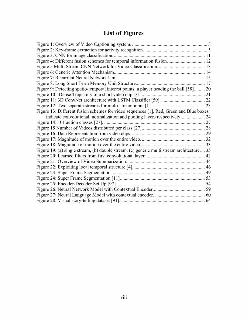
Figure 1: Overview of Video Captioning system. .............................................................. 3Figure 2: Key-frame extraction for activity recognition. .................................................... 5Figure 3: CNN for image classification. ........................................................................... 11Figure 4: Different fusion schemes for temporal information fusion. .............................. 12Figure 5 Multi Stream CNN Network for Video Classification. ...................................... 13Figure 6: Generic Attention Mechanism. .......................................................................... 14Figure 7: Recurrent Neural Network Unit. ....................................................................... 15Figure 8: Long Short Term Memory Unit Structure ......................................................... 17Figure 9: Detecting spatio-temporal interest points: a player heading the ball [58]. ........ 20Figure 10: Dense Trajectory of a short video clip [31]. ................................................... 21Figure 11: 3D ConvNet architecture with LSTM Classifier [59]. .................................... 22Figure 12: Two separate streams for multi-stream input [1]. ........................................... 23Figure 13: Different fusion schemes for video sequences [1]. Red, Green and Blue boxes

indicate convolutional, normalization and pooling layers respectively. ................... 24Figure 14: 101 action classes [27]. ................................................................................... 27Figure 15 Number of Videos distributed per class [27]. ................................................... 28Figure 16: Data Representation from video clips. ............................................................ 29Figure 17: Magnitude of motion over the entire video. .................................................... 32Figure 18: Magnitude of motion over the entire video. .................................................... 33Figure 19: (a) single stream, (b) double stream, (c) generic multi stream architecture. ... 35Figure 20: Learned filters from first convolutional layer. ................................................ 42Figure 21: Overview of Video Summarization. ................................................................ 44Figure 22: Exploiting local temporal structure [4]. .......................................................... 46Figure 23: Super Frame Segmentation. ............................................................................ 49Figure 24: Super Frame Segmentation [11]. ..................................................................... 53Figure 25: Encoder-Decoder Set Up [97]. ........................................................................ 54Figure 26: Neural Network Model with Contextual Encoder. .......................................... 59Figure 27: Neural Language Model with contextual encoder. ......................................... 60Figure 28: Visual story-telling dataset [91]. ..................................................................... 64

ix

List of Tables

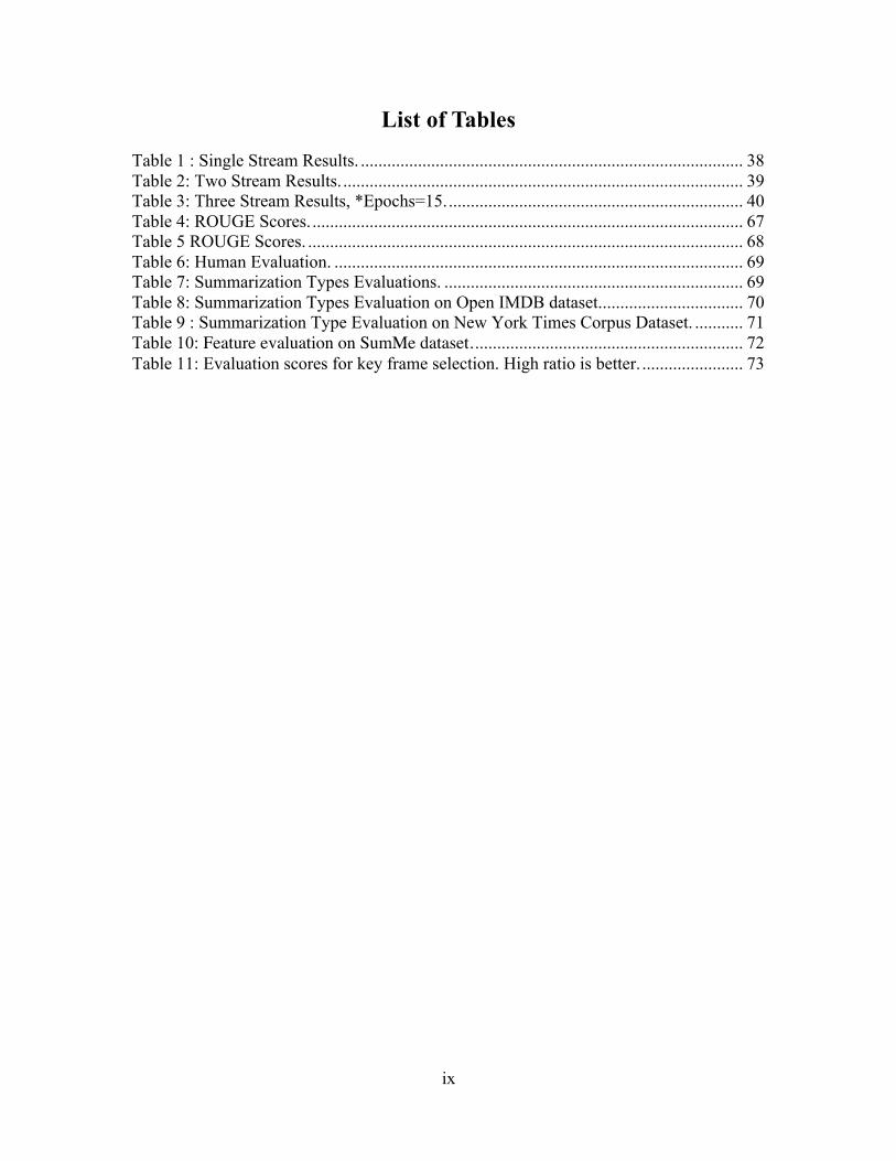
Table 1 : Single Stream Results. ....................................................................................... 38Table 2: Two Stream Results. ........................................................................................... 39Table 3: Three Stream Results, *Epochs=15. ................................................................... 40Table 4: ROUGE Scores. .................................................................................................. 67Table 5 ROUGE Scores. ................................................................................................... 68Table 6: Human Evaluation. ............................................................................................. 69Table 7: Summarization Types Evaluations. .................................................................... 69Table 8: Summarization Types Evaluation on Open IMDB dataset. ................................ 70Table 9 : Summarization Type Evaluation on New York Times Corpus Dataset. ........... 71Table 10: Feature evaluation on SumMe dataset. ............................................................. 72Table 11: Evaluation scores for key frame selection. High ratio is better. ....................... 73

x

Glossary

Term Definition of the term as used in the thesis.

1

Chapter 1 Introduction

Decreasing hardware costs, advanced functionality and prolific use of video

in the judicial system has recently caused video surveillance to spread from

traditional military, retail, and large scale metropolitan applications to

everyday activities. For example, most homeowner security systems come

with video options, cameras in transportation hubs and highways report

congestion, retail surveillance has been expanded for targeted marketing, and

even small suburbs, such as the quiet town of Elk Grove, CA utilize cameras

to detect and deter petty crimes in parks and pathways.

Ease of use, instant sharing, and high image quality have resulted in abundant

amounts video capture not only on social media outlets like Facebook and

YouTube, but also personal devices including cell phones and computers.

Around the world people upload 300 hours of videos per minute just on

YouTube1. If a video is not tagged properly as per the content, it might lose

its usability. Several solutions are available to manage, organize, and search

still images. Applying similar techniques to video works well for short

snippets, but breaks down for videos over a few minutes long. While computer

vision techniques have significantly helped in organizing and searching still

image data, these methods do not scale directly to videos, and are often

computationally inefficient. Videos those are tens of minutes to several hours

long remain a major technical challenge. Ensuring that important moments

are preserved, a proud parent may record long segments of their baby’s first

birthday party. While the videos may have captured cherished moments, they

1 http://www.statisticbrain.com/youtube-statistics/

2

may also include substantial amounts of transition time and irrelevant

imagery.

Natural language summarization of a video has been gaining attention due to

its direct applications in video indexing, automatic movie review generation

and describing movies for visually challenged people. Recent video

captioning frameworks [66, 69] have demonstrated great progress at creating

natural language descriptions of a video clip, but extending such methods to

long videos can be very time and resource consuming. This thesis investigates

captioning video sequences that are several hours long. Popular attention

models are used to identify key segments in a video. Attention models let deep

learning networks focus on a subsection of an input image or video sequence.

This research emphasizes visual attention [5] mechanisms for temporal

attention to identify where to look in time. Such mechanisms can identify key

segments of a video. Key segments are clips extracted from longer videos.

These clips are used to represent nearly all visual information available in

video. Long Short Term Memory (LSTM) units are used to generate a brief

textual description of each segment. Subsequent language models combine

each segment textual description to generate a higher-level text description

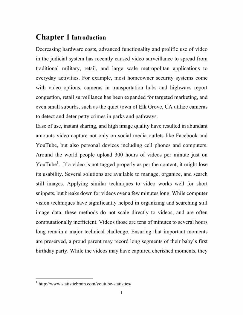
which can summarize the entire video; as shown in Figure 1.

3

Figure 1: Overview of Video Captioning system.

Detection and recognition of objects and activities in video is critical to

expanding the functionality of these systems. Advanced activity

understanding can significantly enhance security details in airports, train

stations, markets, and sports stadiums, and can provide peace of mind to

homeowners, Uber drivers, and officials with body cameras. Security officers

can do an excellent job at detecting and annotating relevant information,

however they simply cannot keep up with the terabytes of video being

uploaded daily. Automated video analytics can be very helpful to organize

and index such very large video repositories. This work scrutinizes every

frame, databasing a plethora of object, activity, and scene based information

for subsequent video analysis. To achieve this goal, there is a substantial need

for the development of effective and efficient automated tools for video

understanding.

To mitigate these problems, we propose techniques that leverage recent

advances in video summarization [15, 26, 48, 49], video annotation [3, 4, 11],

and text summarization [28, 5], to summarize hour long videos to a

substantially short visual and textual summary. Video processing has been

well studied problem in the field of computer vision. Every video analytics

4

solution starts with analyzing each frame and then combine information

gathered from every frame to exploit temporal dependencies. Various video

analytics solutions perform either frame wise analysis or consider collection

of frames as 3D visual data and process the the 3D data. Frame wise analytics

can be either object detection, activity classification, salient feature extraction,

etc. Conventional methods use hand-crafted features such as motion SIFT [17]

or HOG [2] to classify actions, object, scene, etc for each frame. Recent

successes of deep learning [3, 4, 5] in the still image domain have influenced

video research. Researchers have introduced varying color spaces [6], optical

flow [7], and implemented clever architectures [8] to fuse disparate inputs.

This study analyzes the usefulness of the varying input channels, utilizes key

frame extraction for efficacy, identify interesting segments from long videos

using image quality and consumer preference. We smartly pick segments from

longer videos, these segments are feature rich and provide comprehensive

information about entire video. Beforehand computation of these key-

segments is essential because large scale video classification demands

excessive computational requirements. Karpathy et al. [8] proposed several

techniques for fusion of temporal information. However, these techniques

process sample frames selected randomly from full length video. Such random

selection of samples may not consider all useful motion and spatial

information. Simonyan and Zisserman [23] used optical flow to represent the

motion information to achieve high accuracy, but with steep computational

requirements. For example, they reported that the optical flow data on 13K

video snippets was 1.5 TB.

We validated our hypothesis that key-segments save computational

requirements with a series of experiments on the UCF-101 dataset. We first

compute key frames of a video, and then analyze key frames and their

5

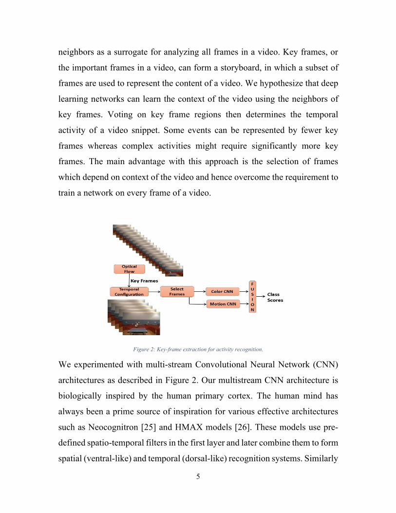
neighbors as a surrogate for analyzing all frames in a video. Key frames, or

the important frames in a video, can form a storyboard, in which a subset of

frames are used to represent the content of a video. We hypothesize that deep

learning networks can learn the context of the video using the neighbors of

key frames. Voting on key frame regions then determines the temporal

activity of a video snippet. Some events can be represented by fewer key

frames whereas complex activities might require significantly more key

frames. The main advantage with this approach is the selection of frames

which depend on context of the video and hence overcome the requirement to

train a network on every frame of a video.

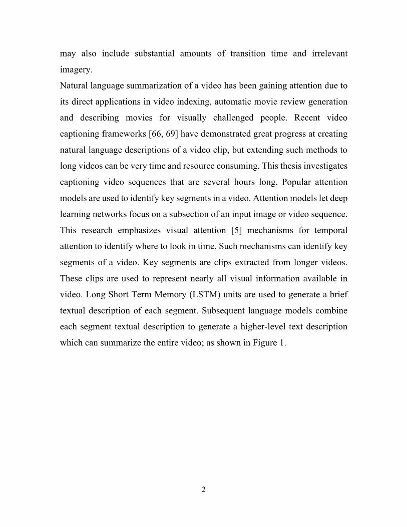
Figure 2: Key-frame extraction for activity recognition.

We experimented with multi-stream Convolutional Neural Network (CNN)

architectures as described in Figure 2. Our multistream CNN architecture is

biologically inspired by the human primary cortex. The human mind has

always been a prime source of inspiration for various effective architectures

such as Neocognitron [25] and HMAX models [26]. These models use pre-

defined spatio-temporal filters in the first layer and later combine them to form

spatial (ventral-like) and temporal (dorsal-like) recognition systems. Similarly

6

in multistream networks, each individual slice of a convolution layer is

dedicated to one type of data representation and passed concurrently with all

other representations.

Our work does not focus on competing state-of-the-art accuracy rather we are

interested in evaluating the architectural performance while combining

different color spaces over key-frame based video frame selection. We

extended the two stream CNN implementation proposed by Simonyan and

Zisserman [23] to a multi-stream architecture. Streams are categorized into

color streams and temporal streams, where color streams are further divided

based on color spaces. The color streams use RGB and YCbCr color spaces.

YCbCr color space has been extremely useful for video/image compression

techniques. In the first spatial stream, we process the luma and chroma

components of the key frames. Chroma components are optionally

downsampled and integrated in the network at a later stage. The architecture

is defined such that both luma and chroma components train a layer of

convolutional filters together as a concatenated array before the fully

connected layers. Apart from color information, optical flow data is used to

represent motion. Optical flow has been a widely accepted representation of

motion, our multi-stream architecture contains dedicated stream for optical

flow data.

This study shows that color and motion cues are necessary and their

combination is preferred for accurate action detection. We studied the

performance of key frames over sequentially selected video clips for large

scale human activity classification. We experimentally support that smartly

selected key frames add valuable data to CNNs and hence perform better than

conventional sequential or randomly selected clips. Using key frames not only

provides better results but can significantly reduce the amount of data being

7

processed. To further reduce computational resources, multi-stream

experiments advocate that lowering down the resolution of chrominance data

stream does not harm performance significantly. Our results indicate that

passing optical flow and YCbCr data into our multistream architecture at key

frame locations of videos offer comprehensive feature learning, which may

lead to better understanding of human activity.

We extended our optical flow based key-frame method with the addition of

interesting segments from long videos using image quality and consumer

preference. Key frames are extracted from interesting segments whereby deep

visual-captioning techniques generate visual and textual summaries. Captions

from interesting segments are fed into extractive methods to generate

paragraph summaries from the entire video. The paragraph summary is

suitable for search and organization of videos, and the individual segment

captions are suitable for efficient seeking to proper temporal offset in long

videos. Because boundary cuts of interesting segments follow

cinematography rules, the concatenation of segments forms a shorter

summary of the long video. Our method provides knobs to increase and/or

decrease both the video and textual summary length to suit the application.

While we evaluate our methods on egocentric videos and TV episodes, similar

techniques can also be used in commercial and government applications such

as sports event summarization or surveillance, security, and reconnaissance.

Text summarization is on-going challenge in the field of natural language

processing. The task of condensed representation of longer text is challenging

due to the demand of huge structured datasets and the necessity to exploit core

story-flow from the unforeseen data. Various past summarization approaches

involve extractive or scoring based summarization systems where individual

confidence scores from parts of text are extracted and stitched together to

8

generate a condensed summary. Whereas, this work is inspired by the recent

success of neural language models and attention based encoders. This

approach is fully data driven and requires less information about sentence

structure. It can learn latent soft story-flow alignment between input text and

generated summaries.

9

Chapter 2 Thesis Objective The Primary objective of this work is to explore efficient solutions for video

activity classification and video to text summarization. Our key-frame

experiments answer the following questions:

• Does the fusion of multiple color spaces perform better than a single-

color space?

• How can one process less amount of data while maintaining model

performance?

• What is the best combination of color spaces and optical flow for better

activity recognition?

We further extend our optical flow based frame selection with various

cinematographical feature scores and temporal attention for video

summarization application. The novel contributions of this research include:

• The ability to split a video into super frame segments, ranking each

segment by image quality, cinematography rules, salient motion and

consumer preference;

• Advancing the field of video annotation by combining recent deep

learning discoveries in image classification, recurrent neural networks,

and transfer learning;

• Adopting textual summarization methods to produce human readable

summaries of video.

• Providing knobs such that both the video and textual summary can be

of variable length.

10

Chapter 3 Background

3.1. Convolutional Neural Networks. Convolutional Neural Networks (CNNs) are a class of neural networks that

have proved very precise not only for image recognition and classification,

but also in complex systems such as identifying faces, image to text

description, Q&A systems, etc. Recent advancements in the field of self-

driving cars, virtual assistants, health care assistants, recommendation

systems, intelligent robots, smart video surveillance, etc. have been entirely

supported by ground breaking successes of CNNs.

CNNs are biologically inspired by the human visual cortex. The human brain

contains billions of neurons connected to each other. These neurons have the

unique functionality of being active/excited for specific visual or any sensory

stimulus. Later, experiments2 show that neurons show plasticity behavior in

their functionality. This means a neuron responsible for being excited after

seeing dogs can be retrained to be excited when seeing cats.

CNNs are a mathematical way to represent these neurons and their

connections. The mathematical representation of neurons involves some

learnable weights and biases. Groups of neurons accepting one kind of input

represent a layer in a CNN network. The entire CNN network contains several

layers, each layer optionally followed by a nonlinear activation function such

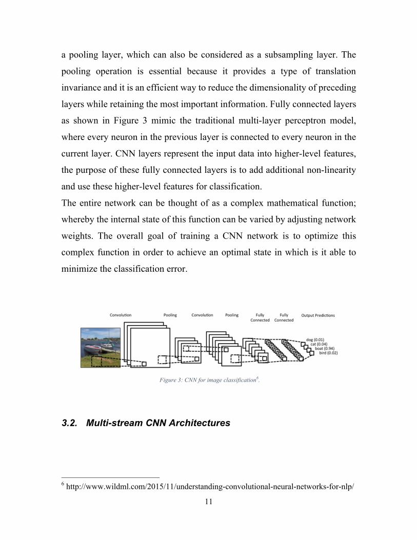
as ReLU3 or tanh4. Figure 3 displays a network diagram of a CNN model5 for

image classification problem. Sometimes a convolutional layer is followed by

2 https://www.linkedin.com/pulse/neuroplasticity-three-easy-experiments-david-orban 3 https://en.wikipedia.org/wiki/Rectifier_(neural_networks) 4 https://theclevermachine.wordpress.com/tag/tanh-function/ 5 http://www.wildml.com/2015/11/understanding-convolutional-neural-networks-for-nlp/

11

a pooling layer, which can also be considered as a subsampling layer. The

pooling operation is essential because it provides a type of translation

invariance and it is an efficient way to reduce the dimensionality of preceding

layers while retaining the most important information. Fully connected layers

as shown in Figure 3 mimic the traditional multi-layer perceptron model,

where every neuron in the previous layer is connected to every neuron in the

current layer. CNN layers represent the input data into higher-level features,

the purpose of these fully connected layers is to add additional non-linearity

and use these higher-level features for classification.

The entire network can be thought of as a complex mathematical function;

whereby the internal state of this function can be varied by adjusting network

weights. The overall goal of training a CNN network is to optimize this

complex function in order to achieve an optimal state in which is it able to

minimize the classification error.

Figure 3: CNN for image classification6.

3.2. Multi-stream CNN Architectures

6 http://www.wildml.com/2015/11/understanding-convolutional-neural-networks-for-nlp/

12

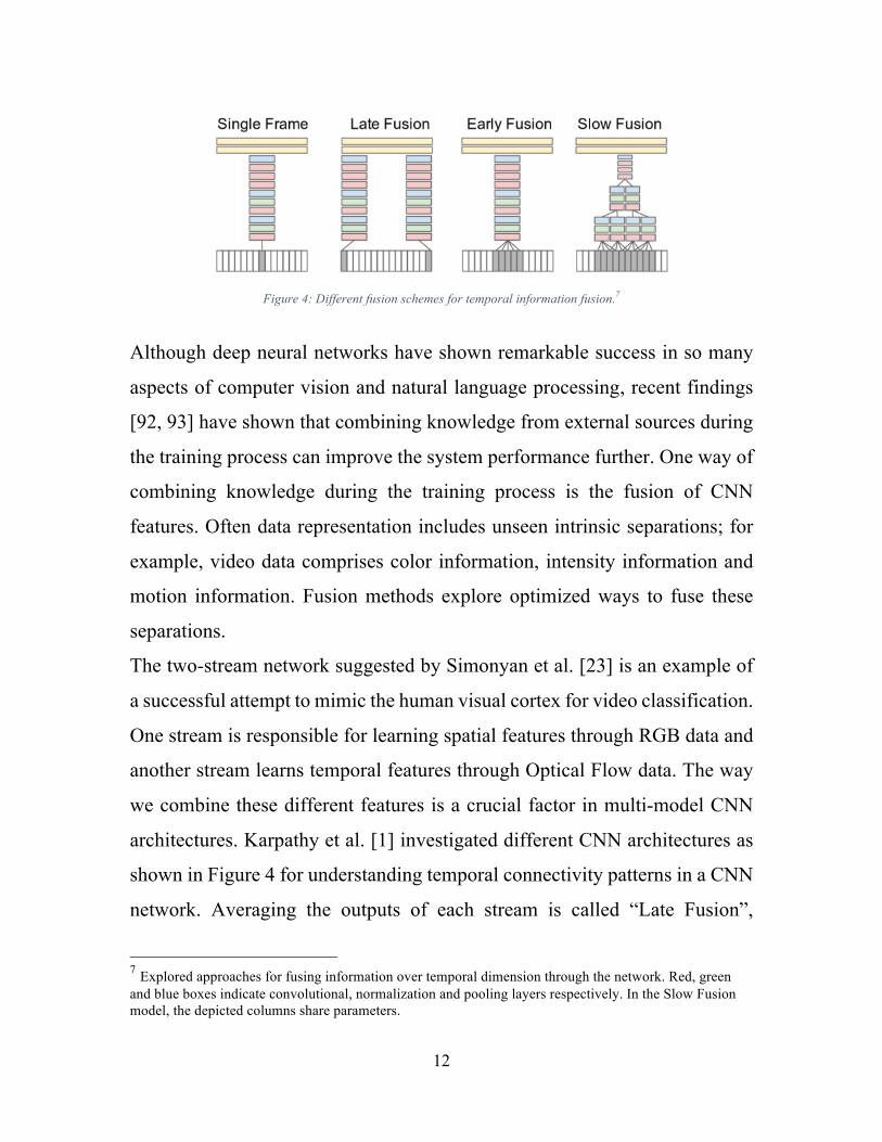
Figure 4: Different fusion schemes for temporal information fusion.7

Although deep neural networks have shown remarkable success in so many

aspects of computer vision and natural language processing, recent findings

[92, 93] have shown that combining knowledge from external sources during

the training process can improve the system performance further. One way of

combining knowledge during the training process is the fusion of CNN

features. Often data representation includes unseen intrinsic separations; for

example, video data comprises color information, intensity information and

motion information. Fusion methods explore optimized ways to fuse these

separations.

The two-stream network suggested by Simonyan et al. [23] is an example of

a successful attempt to mimic the human visual cortex for video classification.

One stream is responsible for learning spatial features through RGB data and

another stream learns temporal features through Optical Flow data. The way

we combine these different features is a crucial factor in multi-model CNN

architectures. Karpathy et al. [1] investigated different CNN architectures as

shown in Figure 4 for understanding temporal connectivity patterns in a CNN

network. Averaging the outputs of each stream is called “Late Fusion”,

7 Explored approaches for fusing information over temporal dimension through the network. Red, green and blue boxes indicate convolutional, normalization and pooling layers respectively. In the Slow Fusion model, the depicted columns share parameters.

13

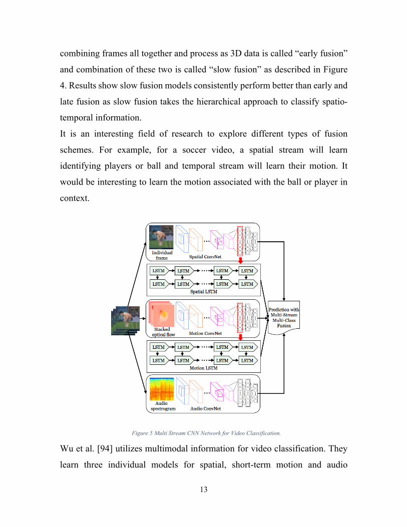
combining frames all together and process as 3D data is called “early fusion”

and combination of these two is called “slow fusion” as described in Figure

4. Results show slow fusion models consistently perform better than early and

late fusion as slow fusion takes the hierarchical approach to classify spatio-

temporal information.

It is an interesting field of research to explore different types of fusion

schemes. For example, for a soccer video, a spatial stream will learn

identifying players or ball and temporal stream will learn their motion. It

would be interesting to learn the motion associated with the ball or player in

context.

Figure 5 Multi Stream CNN Network for Video Classification.

Wu et al. [94] utilizes multimodal information for video classification. They

learn three individual models for spatial, short-term motion and audio

14

information. Outputs from these models are then fused to learn the best set of

weights for action classification with video data.

3.3. Attention Models Attention models are recent trends in deep learning community. Similar to

other deep learning traits, attention mechanism is also biologically inspired by

the human brain’s reaction to visual data. The mammalian brain uses attention

to focus certain parts of the visual input at the same time, giving more or less

emphasis to parts of visual input which are more or less important at a given

point in time. It gives deep learning models the ability to focus on parts that

are giving feature rich information and getting rid of parts contributing less.

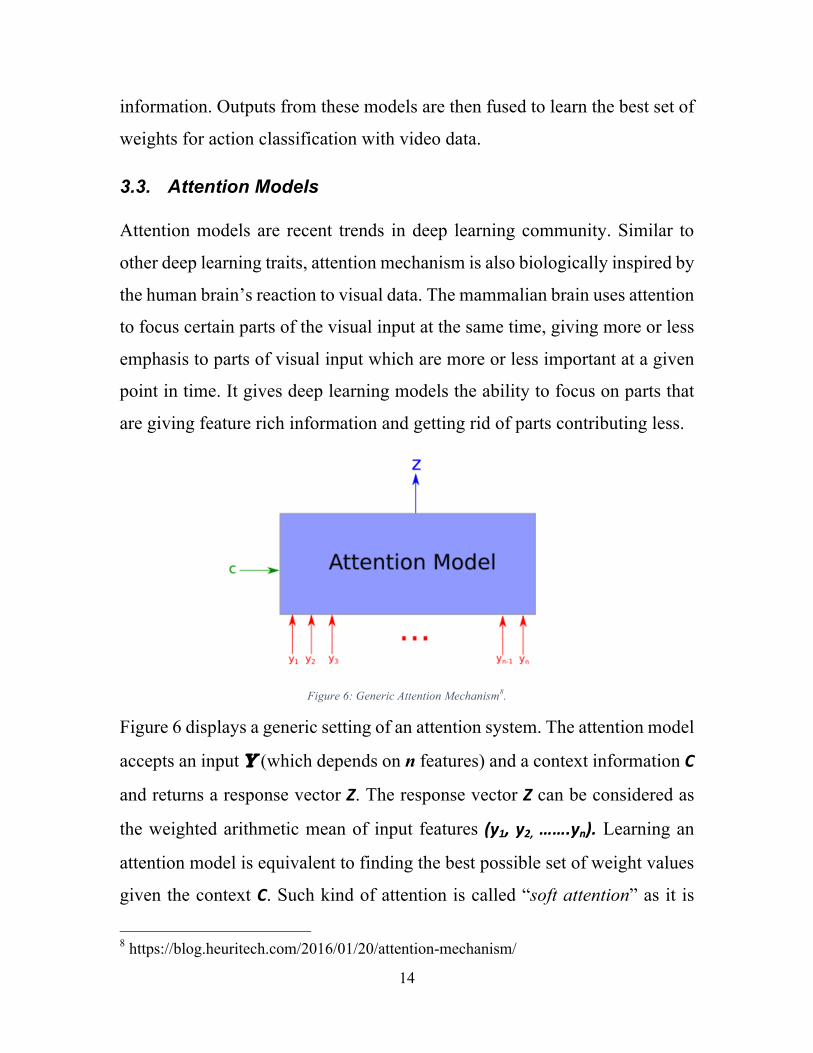
Figure 6: Generic Attention Mechanism8.

Figure 6 displays a generic setting of an attention system. The attention model

accepts an input U (which depends on n features) and a context information C

and returns a response vector Z. The response vector Z can be considered as

the weighted arithmetic mean of input features (y1,y2,…….yn). Learning an

attention model is equivalent to finding the best possible set of weight values

given the context C. Such kind of attention is called “soft attention” as it is

8 https://blog.heuritech.com/2016/01/20/attention-mechanism/

15

fully differentiable where gradients can propagate through the entire network.

A stochastic way of dealing with this problem is called “hard attention”.

Instead of forming a linear combination of all the feature points, it selects one

single sample yi (out of n) and the associated probability Pi to propagate the

gradients. Recent research has been favored to soft attention as it is completely

differentiable process instead of relying on a stochastic approach.

3.4. Recurrent Neural Networks

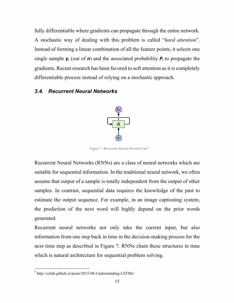
Figure 7: Recurrent Neural Network Unit.9

Recurrent Neural Networks (RNNs) are a class of neural networks which are

suitable for sequential information. In the traditional neural network, we often

assume that output of a sample is totally independent from the output of other

samples. In contrast, sequential data requires the knowledge of the past to

estimate the output sequence. For example, in an image captioning system,

the prediction of the next word will highly depend on the prior words

generated.

Recurrent neural networks not only take the current input, but also

information from one step back in time in the decision-making process for the

next time step as described in Figure 7. RNNs chain these structures in time

which is natural architecture for sequential problem solving.

9 http://colah.github.io/posts/2015-08-Understanding-LSTMs/

16

3.5. Long Short Term Memory Units One major problem with RNNs is the “vanishing gradient problem”. We

assume that RNNs can encapsulate the entire history of all past time steps in

order to compute the next step. If the history goes more than a handful steps

in time, RNNs are often prone to show unusual results. At each time step,

gradients express the change in weights with regards to the change in error.

Backpropagation involves multiplication of these gradients as we go back in

time. As we keeping multiplying consecutive small numbers (<1), the result

becomes considerably small. Such gradients often become too small for

computers to work with or even for a network to learn. At the point, back in

time when gradients become small, those associated weights contribute very

little or nothing to the current task of computing the next time step. Therefore,

RNNs sometime struggle to take advantage of long term dependencies. This

problem is termed as the Vanishing Gradient Problem as first identified by

Bengio et al. [95].

In the mid-90s, Hochreiter et al. [96] introduced a variation of RNNs named

Long Short Term Memory units (LSTMs). LSTMs offered a solution to the

vanishing gradient problem. LSTM worked really well with variety of

problems and are currently widely used in sequence modeling.

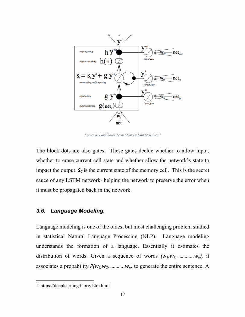
The key to LSTMs are gated cell structures which are responsible to control

the information flow inside the network as shown in Figure 8. By opening and

closing operations of these gates, the network can decide which information

to store, read or write, which information to block and which information to

pass. At the bottom of Figure 8, there are three inputs fed to the network and

also to three gates on the right side. Arrows contain present input and past

state of the network.

17

Figure 8: Long Short Term Memory Unit Structure10

The block dots are also gates. These gates decide whether to allow input,

whether to erase current cell state and whether allow the network’s state to

impact the output. SC is the current state of the memory cell. This is the secret

sauce of any LSTM network- helping the network to preserve the error when

it must be propagated back in the network.

3.6. Language Modeling.

Language modeling is one of the oldest but most challenging problem studied

in statistical Natural Language Processing (NLP). Language modeling

understands the formation of a language. Essentially it estimates the

distribution of words. Given a sequence of words (w1,w2, ………..wn), it

associates a probability P(w1,w2,………..wn) to generate the entire sentence. A

10 https://deeplearning4j.org/lstm.html

18

language modeling problem always starts with having a lot of text information

in the corresponding language. Further, we define a vocabulary of given text

V. This vocabulary contains all the words present in the text. In English, the

vocabulary can be something like this

V = {person, dog, car, walking, …………….., guitar, rain}

In general, V is quite large as it may contain almost every occurring word in

the language- but it is a finite set. A sentence will be sequence of words taken

from a vocabulary. According to the definition11 “A language model consists

of a finite set V and a function p(x1,…….xn) such that:

• For any <x1,…….xn>ÎV,p(x1,…….xn)³0

• In addition,

p(x1, …… . xn)<+,,…….+->Î.

= 1

(3.1)

Therefore, p(x1,…….xn) is a probability distribution over the sentences formed

by vocabulary set V.

11 http://www.cs.columbia.edu/~mcollins/lm-spring2013.pdf

19

Chapter 4 Key Frame Segmentation and Multi-

Stream CNNs Surveillance cameras have become big business, with most metropolitan cities

spending millions of dollars to watch residents, both from street corners,

public transportation hubs, and body cameras on officials. Watching and

processing the petabytes of streaming video is a daunting task, making auto-

mated and user assisted methods of searching and understanding videos

critical to their success. Although numerous techniques have been developed,

large scale video classification remains a difficult task due to excessive

computational requirements.

In this work, we conduct an in-depth study to investigate effective

architectures and semantic features for efficient and accurate solutions to

activity recognition. We investigate different color spaces, optical flow, and

introduce a novel deep learning fusion architecture for multi-modal inputs.

The introduction of key frame extraction, instead of using every frame or a

random representation of video data, make our methods computationally

tractable. Results further indicate that transforming the image stream into a

compressed color space reduces computational requirements with minimal

effect on accuracy.

4.1. Past Work Video classification has been a longstanding research topic in the multimedia

processing and computer vision fields. Efficient and accurate classification

performance relies on the extraction of salient video features. Conventional

methods for video classification [53] involve generation of video descriptors

20

that encode both spatial and motion variance information into hand-crafted

features such as Histogram of Oriented Gradients (HOG) [18], Histogram of

Optical Flow (HOF) [28], and spatio-temporal interest points [55]. These

features are then encoded as a global representation through a bag of words

[29] or fisher vector based encoding [30] and then passed to a classifier [31].

Bag-of-words is popular approach in video processing where each feature is

placed into quantized buckets of features. These buckets are learned through

K-means or other popular clustering algorithms. Later, a classifier is trained

to classify these bag-of-words representation of video data to ground truth

classes. These feature extraction methods along with classification methods

such as SVMs produced state-of-the-art methods for image classification

before the deep learning boom. Various image features have been extended to

video data such as 3D-SIFT [55], 3D-HOG [56] and extended SURF[57].

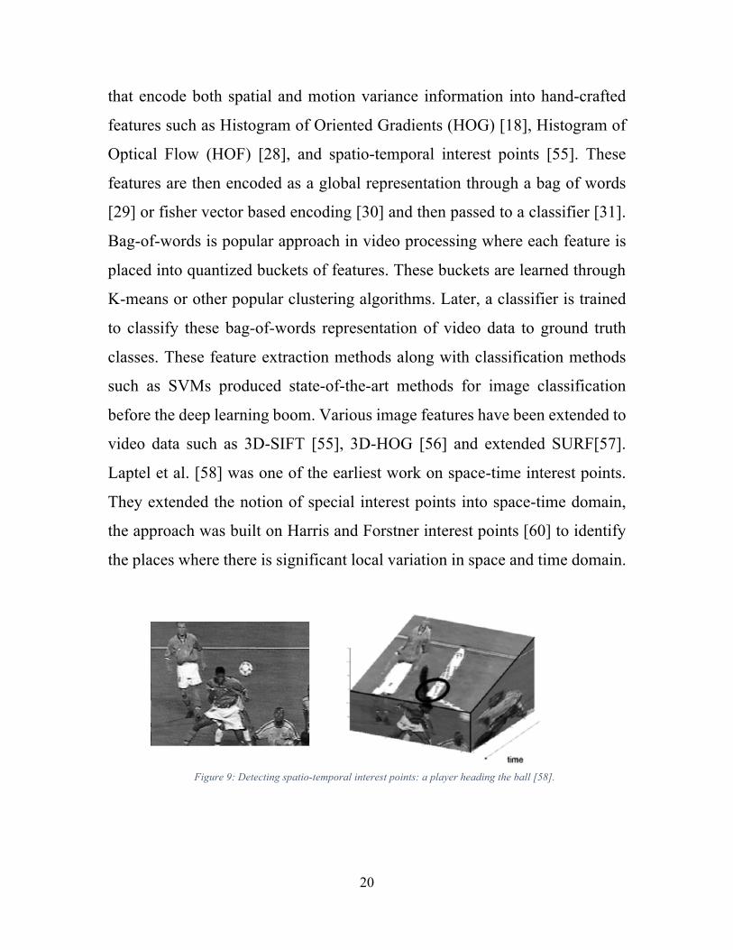
Laptel et al. [58] was one of the earliest work on space-time interest points.

They extended the notion of special interest points into space-time domain,

the approach was built on Harris and Forstner interest points [60] to identify

the places where there is significant local variation in space and time domain.

Figure 9: Detecting spatio-temporal interest points: a player heading the ball [58].

21

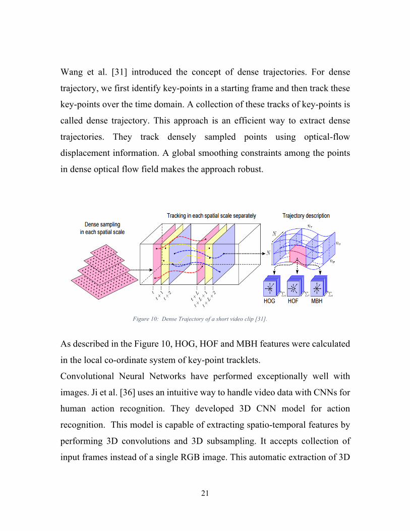
Wang et al. [31] introduced the concept of dense trajectories. For dense

trajectory, we first identify key-points in a starting frame and then track these

key-points over the time domain. A collection of these tracks of key-points is

called dense trajectory. This approach is an efficient way to extract dense

trajectories. They track densely sampled points using optical-flow

displacement information. A global smoothing constraints among the points

in dense optical flow field makes the approach robust.

Figure 10: Dense Trajectory of a short video clip [31].

As described in the Figure 10, HOG, HOF and MBH features were calculated

in the local co-ordinate system of key-point tracklets.

Convolutional Neural Networks have performed exceptionally well with

images. Ji et al. [36] uses an intuitive way to handle video data with CNNs for

human action recognition. They developed 3D CNN model for action

recognition. This model is capable of extracting spatio-temporal features by

performing 3D convolutions and 3D subsampling. It accepts collection of

input frames instead of a single RGB image. This automatic extraction of 3D

22

features was shown to outperform prior action recognition methods on

TRECVID12 and KTH13 action datasets.

Gkioxari and Malik [41] extend the concept of interesting points into regions.

They first detect image regions which are more motion salient and likely to

have objects and actions. Further temporal connection of these features

extracts a spatio-temporal tube like structure. Around 2011 timeframe, deep

models were developing interest in 3D vision community. These models are

able to learn multiple level of feature hierarchies and extract useful features

automatically. M. Baccouche et al. [59] produced very inspiring work of using

two-steps of neural-based deep models for human action recognition. This

work introduced the concept of 3D CNN features with recurrent neural

networks even before the historical Alexnet [19] work.

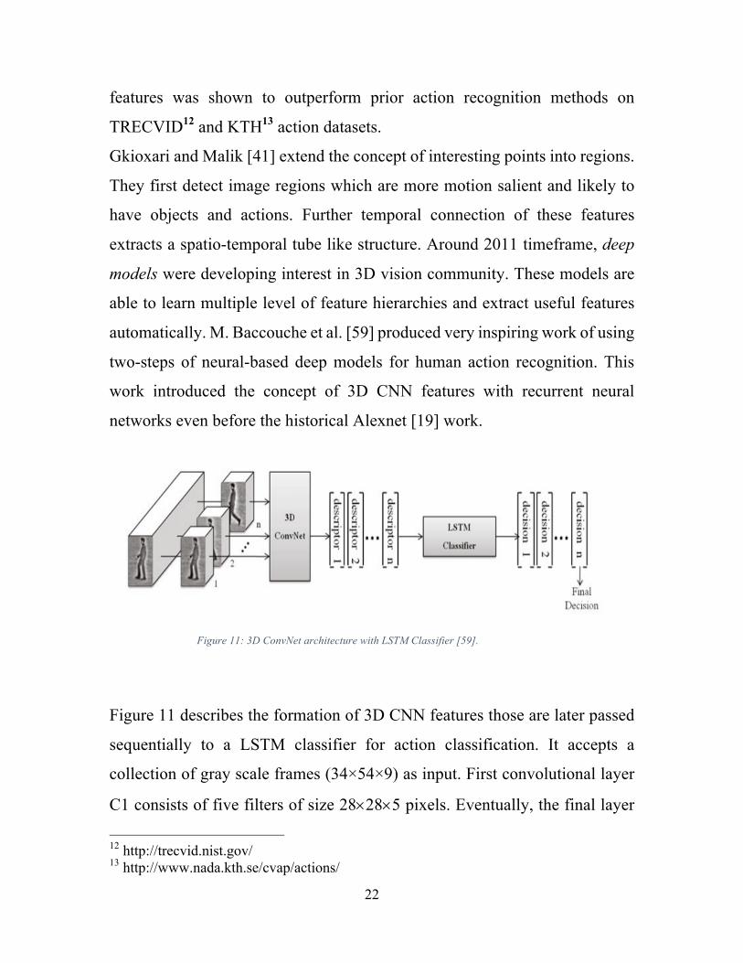
Figure 11: 3D ConvNet architecture with LSTM Classifier [59].

Figure 11 describes the formation of 3D CNN features those are later passed

sequentially to a LSTM classifier for action classification. It accepts a

collection of gray scale frames (34×54×9) as input. First convolutional layer

C1 consists of five filters of size 28´28´5 pixels. Eventually, the final layer

12 http://trecvid.nist.gov/ 13 http://www.nada.kth.se/cvap/actions/

23

C3 consist of five feature maps of size 3´8´1 encoding the input raw data to

a vector of size 120. This vector can be used as salient spatio-temporal feature

for a nine frame video clip. Later, these spatio-temporal features extracted

from different parts of video were passed into a Recurrent Neural Network

architecture with one hidden layer of LSTM cells. Such an arrangement

outperformed action recognition on the KTH1 and KTH2 datasets. These

datasets contain only gray scale video frames; it will be interesting to perform

these experiments with RGB video data. Additionally, KTH1 and KTH2

datasets are small and contain videos from a narrow domain range. One of the

first large scale video classification efforts was done by Karpathy et al. [1].

They provide an in-depth study about CNNs performance for large-scape

video classification with various deep learning fusion architectures.

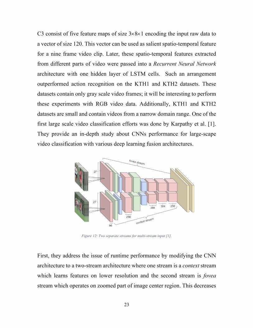
Figure 12: Two separate streams for multi-stream input [1].

First, they address the issue of runtime performance by modifying the CNN

architecture to a two-stream architecture where one stream is a context stream

which learns features on lower resolution and the second stream is fovea

stream which operates on zoomed part of image center region. This decreases

24

the total input dimensionality by the factor of two. Such design takes the

advantage of camera bias problem; where the video camera is focused on

object in center. Later, activations output from each stream are concatenated

just before the fully connected layer. This set up increases the runtime

performance by the factor of 2.4 due to the lower dimensional input data while

keeping the classification accuracy same. The biggest question with video

processing is, how to combine information in temporal dimension? A naïve

approach is to use a voting scheme to vote for features over different parts of

video. Voting takes the holistic representation of video data but it does not

connect information with variable temporal distance. Karpathy et al. [1]

Describes multiple ways to connect temporal information by experimenting

with various deep learning architectures.

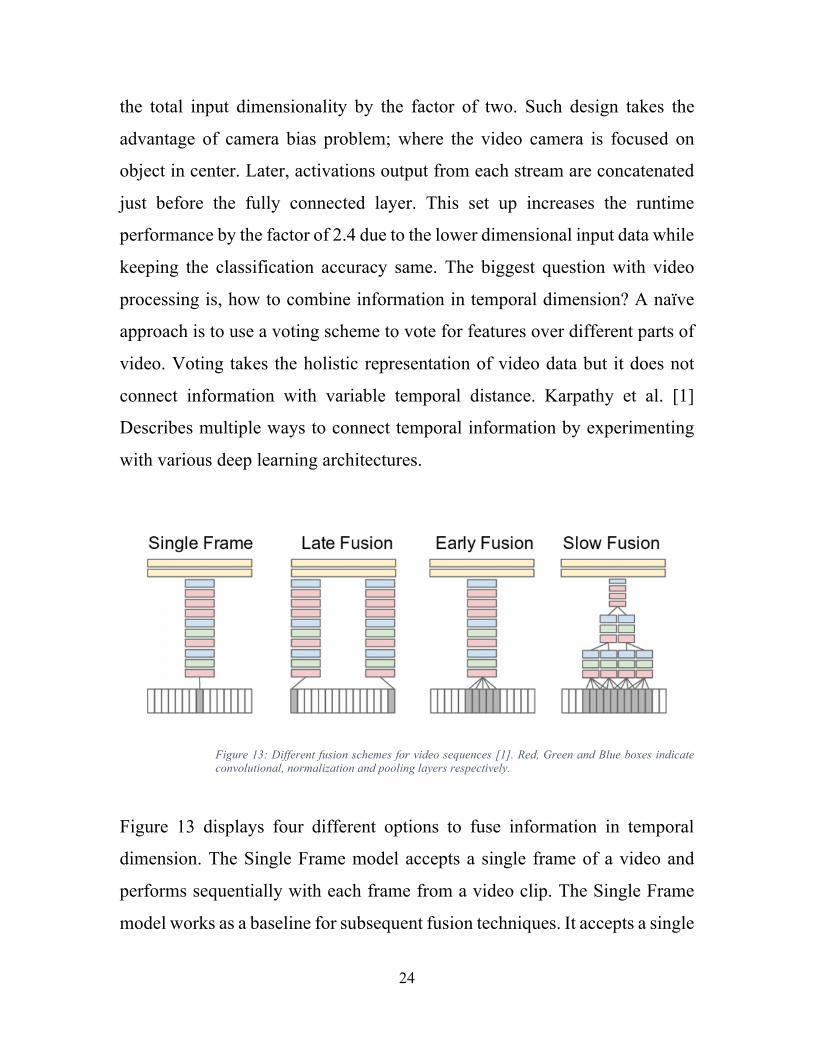
Figure 13: Different fusion schemes for video sequences [1]. Red, Green and Blue boxes indicate convolutional, normalization and pooling layers respectively.

Figure 13 displays four different options to fuse information in temporal

dimension. The Single Frame model accepts a single frame of a video and

performs sequentially with each frame from a video clip. The Single Frame

model works as a baseline for subsequent fusion techniques. It accepts a single

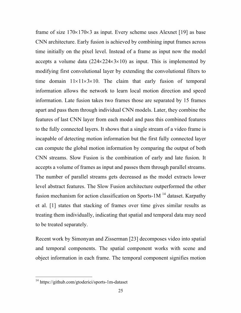
25

frame of size 170´170´3 as input. Every scheme uses Alexnet [19] as base

CNN architecture. Early fusion is achieved by combining input frames across

time initially on the pixel level. Instead of a frame as input now the model

accepts a volume data (224´224´3´10) as input. This is implemented by

modifying first convolutional layer by extending the convolutional filters to

time domain 11´11´3´10. The claim that early fusion of temporal

information allows the network to learn local motion direction and speed

information. Late fusion takes two frames those are separated by 15 frames

apart and pass them through individual CNN models. Later, they combine the

features of last CNN layer from each model and pass this combined features

to the fully connected layers. It shows that a single stream of a video frame is

incapable of detecting motion information but the first fully connected layer

can compute the global motion information by comparing the output of both

CNN streams. Slow Fusion is the combination of early and late fusion. It

accepts a volume of frames as input and passes them through parallel streams.

The number of parallel streams gets decreased as the model extracts lower

level abstract features. The Slow Fusion architecture outperformed the other

fusion mechanism for action classification on Sports-1M 14 dataset. Karpathy

et al. [1] states that stacking of frames over time gives similar results as

treating them individually, indicating that spatial and temporal data may need

to be treated separately.

Recent work by Simonyan and Zisserman [23] decomposes video into spatial

and temporal components. The spatial component works with scene and

object information in each frame. The temporal component signifies motion

14 https://github.com/gtoderici/sports-1m-dataset

26

across frames. Ng et al. [23] evaluated the effect of different color space

representations on the classification of gender. Interestingly, they presented

that gray scale performed better than RGB and YCbCr spaces. Very recent

work by Tran et al. [61] proposes that 3D ConvNets are suitable for spatio-

temporal feature learning whereby a small size (3´3´3) convolutional kernel

outperforms a best performing 3D ConvNet. They [61] named these learnt

features as C3D (Convolutional 3D). These C3D features are current-state-

of-the-art spatio-temporal features for variety of video processing

applications. A simple linear classifier proceeded after C3D gives significant

results for action classification with UCF-101 dataset.

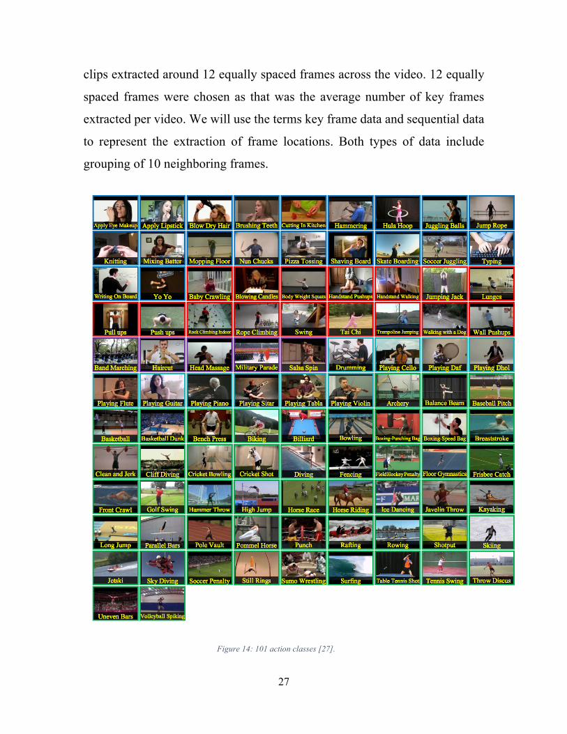
4.2. Dataset Experiments were performed on UCF-101 [27], one of the largest annotated

video datasets with 101 different human actions. It contains 13K videos,

comprising 27 hours of video data. The dataset contains realistic videos with

natural variance in camera motion, object appearance, pose and object scale.

It is a challenging dataset composed of unconstrained videos downloaded

from YouTube which incorporate real world challenges such as poor lighting,

cluttered background and severe camera motion. Video clips from single class

were divided into 25 groups, video clips in a group share some common

information such as same background, same person, same environment, etc.

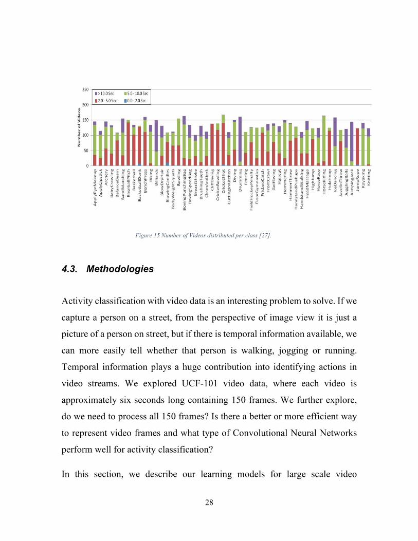
The number of videos per class is reasonably distributed as shown in Figure

15. Every clip has fixed framerate of 25 FPS with resolution of 320´240

pixels. Average video length for UCF-101 is 6.6 seconds. We used UCF-101

split-1 to validate our methodologies. Experiments deal with two classes of

data representation: key frame data and sequential data. Key frame data

includes clips extracted around key frames where sequential data signifies 12

27

clips extracted around 12 equally spaced frames across the video. 12 equally

spaced frames were chosen as that was the average number of key frames

extracted per video. We will use the terms key frame data and sequential data

to represent the extraction of frame locations. Both types of data include

grouping of 10 neighboring frames.

Figure 14: 101 action classes [27].

28

Figure 15 Number of Videos distributed per class [27].

4.3. Methodologies Activity classification with video data is an interesting problem to solve. If we

capture a person on a street, from the perspective of image view it is just a

picture of a person on street, but if there is temporal information available, we

can more easily tell whether that person is walking, jogging or running.

Temporal information plays a huge contribution into identifying actions in

video streams. We explored UCF-101 video data, where each video is

approximately six seconds long containing 150 frames. We further explore,

do we need to process all 150 frames? Is there a better or more efficient way

to represent video frames and what type of Convolutional Neural Networks

perform well for activity classification?

In this section, we describe our learning models for large scale video

29

classification including pre-processing, multi- stream CNN, key frame

selection and the training procedure in detail. At test time, only the key frames

of a test video are passed through the CNN and classified into one of the

activities. This helps to not only show that key frames are capturing the

important parts of the video but also that the testing is faster as compared to

passing all frames though the CNN. A video clip passed through our trained

model gives a certain output. We named this output of a clip “clip level

output”. Voting amongst clip level outputs over the entire length of video

gives us “video level output”. In this work, we present accuracy on both levels.

4.3.1 Early Fusion

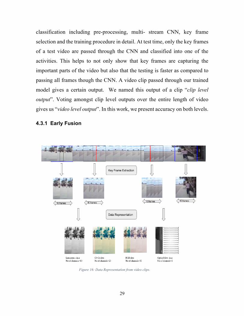
Figure 16: Data Representation from video clips.

30

The early fusion technique combines the entire 10 frame time window of the

filters from the first convolution layer of the CNN. We adapt the time

constraint by modifying the dimension of these filters as F×F×CT, where F

is the filter dimension, T is the time window (10) and C is the number of

channels in the input (3 for RGB). This is an alternate representation from the

more common 4-dimensional convolution.

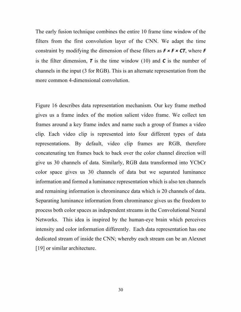
Figure 16 describes data representation mechanism. Our key frame method

gives us a frame index of the motion salient video frame. We collect ten

frames around a key frame index and name such a group of frames a video

clip. Each video clip is represented into four different types of data

representations. By default, video clip frames are RGB, therefore

concatenating ten frames back to back over the color channel direction will

give us 30 channels of data. Similarly, RGB data transformed into YCbCr

color space gives us 30 channels of data but we separated luminance

information and formed a luminance representation which is also ten channels

and remaining information is chrominance data which is 20 channels of data.

Separating luminance information from chrominance gives us the freedom to

process both color spaces as independent streams in the Convolutional Neural

Networks. This idea is inspired by the human-eye brain which perceives

intensity and color information differently. Each data representation has one

dedicated stream of inside the CNN; whereby each stream can be an Alexnet

[19] or similar architecture.

31

4.3.2 Color Stream

Video data can be naturally decomposed into spatial and temporal

information. The most common spatial representation of video frames is the

RGB (3-channel) data. In this study, we compare RGB performance with the

Luminance and Chrominance color space and their combinations thereof.

YCbCr space separates the color into the luminance channel (Y), the blue-

difference channel (Cb), and the red-difference channel (Cr).

Color stream of the architecture accept spatial information of the video data.

The spatial representation of the activity contains global scene and object

attributes such as shape, color and texture. The CNN filters in the color stream

learn the color and edge features from the scene. The human visual system

has lower acuity for color differences than luminance detail. Image and video

compression techniques take advantage of this phenomenon, where the

conversion of RGB primaries to luma and chroma allow for chroma sub-

sampling. We use this concept while formulating our multi-stream CNN

architectures. We sub-sample the chrominance channels by factors of 4 and

16 to test the contribution of color to the framework.

4.3.3 Motion Stream Motion is an intrinsic property of a video that describes an action by a

sequence of frames, where the optical flow could depict the motion of

temporal change. We use an OpenCV implementation [40] of optical flow to

estimate motion in a video. Similar to Gkioxari et al. [25], we stack the optical

32

flow in the x- and y- directions. We scale these by a factor of 16 and stack the

magnitude as the third channel.

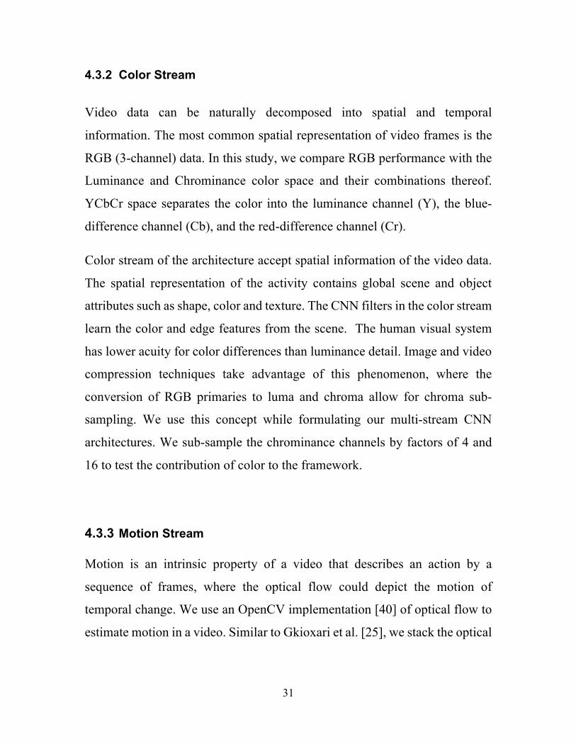
4.3.4 Key Frame Extraction We use the optical flow displacement fields between consecutive frames and

detect motion stillness to identify key frames. A hierarchical time constraint

ensures that fast movement activities are not omitted. The first step in

identifying key frames is the calculation of optical flow for the entire video

and estimate the magnitude of motion using a motion metric as a function of

time [12].

Figure 17: Magnitude of motion over the entire video.

33

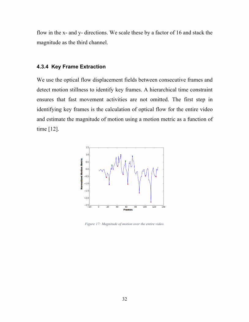
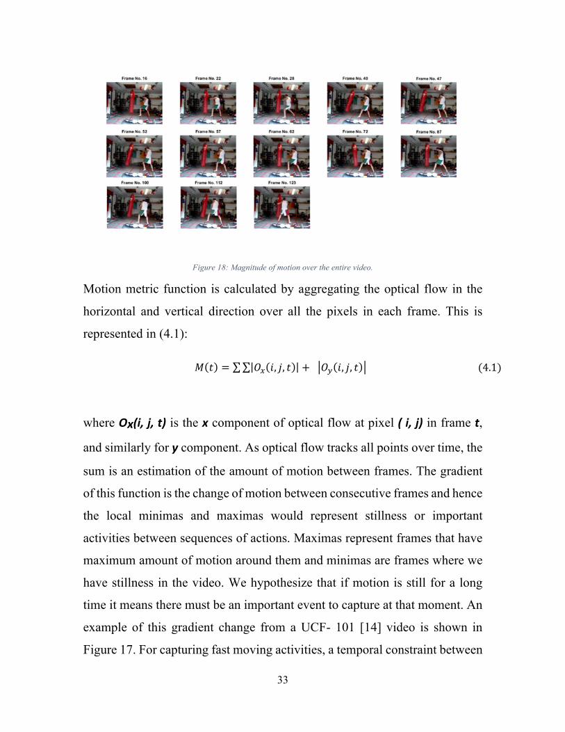
Figure 18: Magnitude of motion over the entire video.

Motion metric function is calculated by aggregating the optical flow in the

horizontal and vertical direction over all the pixels in each frame. This is

represented in (4.1):

𝑀 𝑡 = 𝑂3 𝑖, 𝑗, 𝑡 + 𝑂7 𝑖, 𝑗, 𝑡 (4.1)

where Ox(i,j,t) is the x component of optical flow at pixel (i,j) in frame t,

and similarly for y component. As optical flow tracks all points over time, the

sum is an estimation of the amount of motion between frames. The gradient

of this function is the change of motion between consecutive frames and hence

the local minimas and maximas would represent stillness or important

activities between sequences of actions. Maximas represent frames that have

maximum amount of motion around them and minimas are frames where we

have stillness in the video. We hypothesize that if motion is still for a long

time it means there must be an important event to capture at that moment. An

example of this gradient change from a UCF- 101 [14] video is shown in

Figure 17. For capturing fast moving activities, a temporal constraint between

34

two selected frames is applied during selection [28], which evenly distributes

the important frames over the video length. Frames are dynamically selected

depending on the content of the video. Hence, complex activities or events

would have more key frames, whereas simpler ones may have less.

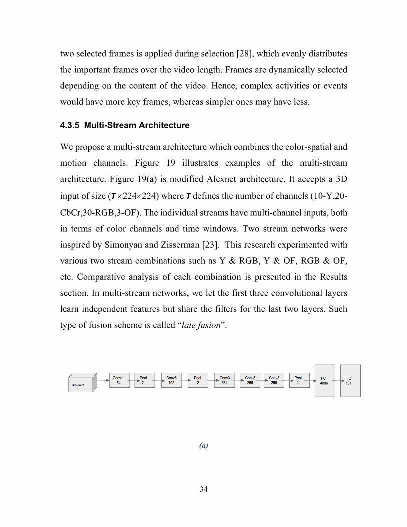
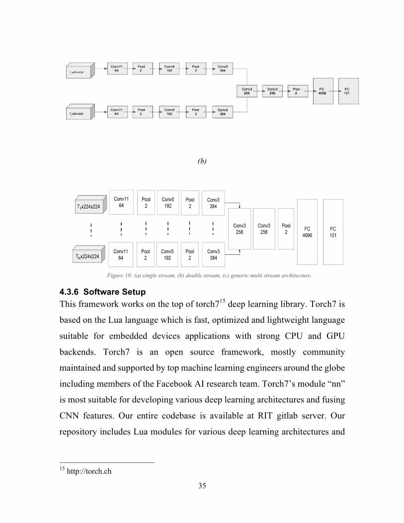
4.3.5 Multi-Stream Architecture We propose a multi-stream architecture which combines the color-spatial and

motion channels. Figure 19 illustrates examples of the multi-stream

architecture. Figure 19(a) is modified Alexnet architecture. It accepts a 3D

input of size (T ´224´224) where T defines the number of channels (10-Y,20-

CbCr,30-RGB,3-OF). The individual streams have multi-channel inputs, both

in terms of color channels and time windows. Two stream networks were

inspired by Simonyan and Zisserman [23]. This research experimented with

various two stream combinations such as Y & RGB, Y & OF, RGB & OF,

etc. Comparative analysis of each combination is presented in the Results

section. In multi-stream networks, we let the first three convolutional layers

learn independent features but share the filters for the last two layers. Such

type of fusion scheme is called “late fusion”.

(a)

35

(b)

Figure 19: (a) single stream, (b) double stream, (c) generic multi stream architecture.

4.3.6 Software Setup This framework works on the top of torch715 deep learning library. Torch7 is

based on the Lua language which is fast, optimized and lightweight language

suitable for embedded devices applications with strong CPU and GPU

backends. Torch7 is an open source framework, mostly community

maintained and supported by top machine learning engineers around the globe

including members of the Facebook AI research team. Torch7’s module “nn”

is most suitable for developing various deep learning architectures and fusing

CNN features. Our entire codebase is available at RIT gitlab server. Our

repository includes Lua modules for various deep learning architectures and

15 http://torch.ch

36

Python modules for optical flow computation with video frames. Optical flow

was calculated using the Python front end to OpenCV. The step-by-step

process to train our CNN network is as follows:

1. Install torch7, also install luarocks package manager to install other

dependencies.

1.1 . Torch installation:

1.1.1 git clone https://github.com/torch/distro.git~/torch --recursive

1.1.2 cd ~/torch; bash install-deps;

1.1.3 ./install.sh

1.2 . Other dependencies installation:

1.2.1 luarocks install package-name

2. Git clone video classification repository with following link:

git@kgcoe-git.rit.edu:sk1846/Video_Classif.git

3. This repository contains directories named as Y, YCbCr, YRGB, etc.

For example, Y and RGB represent a single stream CNN network,

where as YCbCr and YOF signify a two stream CNN network.

4. Inside each directory there are four major “lua” scripts:

a. dataset.lua: This creates a dataset class to perform various

operations such as data pre-processing, batch processing, etc.

b. donkey.lua: Performs data fetching operations on dataset

object.

c. opt.lua: Stores all the model parameters and flags.

d. main.lua: This calls train/test scripts.

4.3.7 Training As discussed, our baseline architecture is similar to [13], but accepts inputs

with multiple stacked frames. Consequently, our CNN models accept data,

37

which has temporal information stored in the third dimension. For example,

the luminance stream accepts input as a short clip of dimensions 224×224×10.

The architecture can be represented as C(64,11,4)-BN-P-C(192,5,1)-BN-P-

C(384,3,1)-BN-C(256,3,1)-BN-P-FC(4096)-FC(4096), where C(d,f,s)

indicates a convolution layer with d number of filters of size f×f with stride

of s. P signifies max pooling layer with 3×3 region and stride of 2. BN denotes

batch normalization [44] layers. The learning rate was initialized at 0.001 and

adaptively gets updated based on the loss per mini batch. The momentum and

weight decay were 0.9 and 5e−4, respectively.

The native resolution of the videos was 320 × 240. Each frame was center

cropped to 240 × 240, then resized to 224 × 224. Each sample was normalized

by mean subtraction and divided by standard deviation across all channels.

4.4. Results We demonstrate our key frame methods for activity classification on the UCF-

101 dataset. We further compare key frame results with sequentially

separated video data. We explored different color spaces and their

combination for multi-stream CNN architectures.

4.4.1 Evaluation The model generates a predicted activity at each selected frame location, and

voting amongst all locations in a video clip is used for video level accuracy.

Although transfer learning boosted RGB and optical flow data performance,

no high performing YCbCr transfer learning models were available. To ensure

fair comparison among methods, all model results were initialized with

38

random weights.

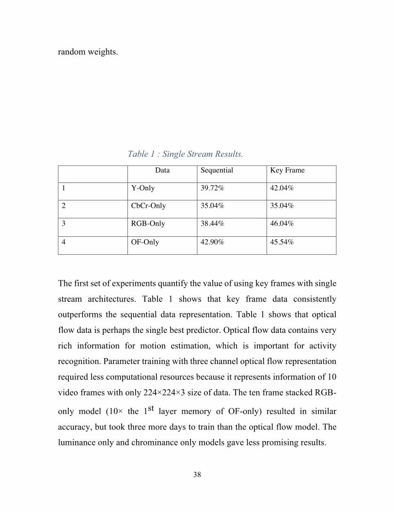
Table 1 : Single Stream Results.

Data Sequential Key Frame

1 Y-Only 39.72% 42.04%

2 CbCr-Only 35.04% 35.04%

3 RGB-Only 38.44% 46.04%

4 OF-Only 42.90% 45.54%

The first set of experiments quantify the value of using key frames with single

stream architectures. Table 1 shows that key frame data consistently

outperforms the sequential data representation. Table 1 shows that optical

flow data is perhaps the single best predictor. Optical flow data contains very

rich information for motion estimation, which is important for activity

recognition. Parameter training with three channel optical flow representation

required less computational resources because it represents information of 10

video frames with only 224×224×3 size of data. The ten frame stacked RGB-

only model (10× the 1st layer memory of OF-only) resulted in similar

accuracy, but took three more days to train than the optical flow model. The

luminance only and chrominance only models gave less promising results.

39

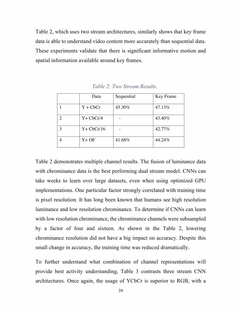
Table 2, which uses two stream architectures, similarly shows that key frame

data is able to understand video content more accurately than sequential data.

These experiments validate that there is significant informative motion and

spatial information available around key frames.

Table 2: Two Stream Results.

Data Sequential Key Frame

1 Y + CbCr 45.30% 47.13%

2 Y+ CbCr/4 - 43.40%

3 Y+ CbCr/16 - 42.77%

4 Y+ OF 41.68% 44.24%

Table 2 demonstrates multiple channel results. The fusion of luminance data

with chrominance data is the best performing dual stream model. CNNs can

take weeks to learn over large datasets, even when using optimized GPU

implementations. One particular factor strongly correlated with training time

is pixel resolution. It has long been known that humans see high resolution

luminance and low resolution chrominance. To determine if CNNs can learn

with low resolution chrominance, the chrominance channels were subsampled

by a factor of four and sixteen. As shown in the Table 2, lowering

chrominance resolution did not have a big impact on accuracy. Despite this

small change in accuracy, the training time was reduced dramatically.

To further understand what combination of channel representations will

provide best activity understanding, Table 3 contrasts three stream CNN

architectures. Once again, the usage of YCbCr is superior to RGB, with a

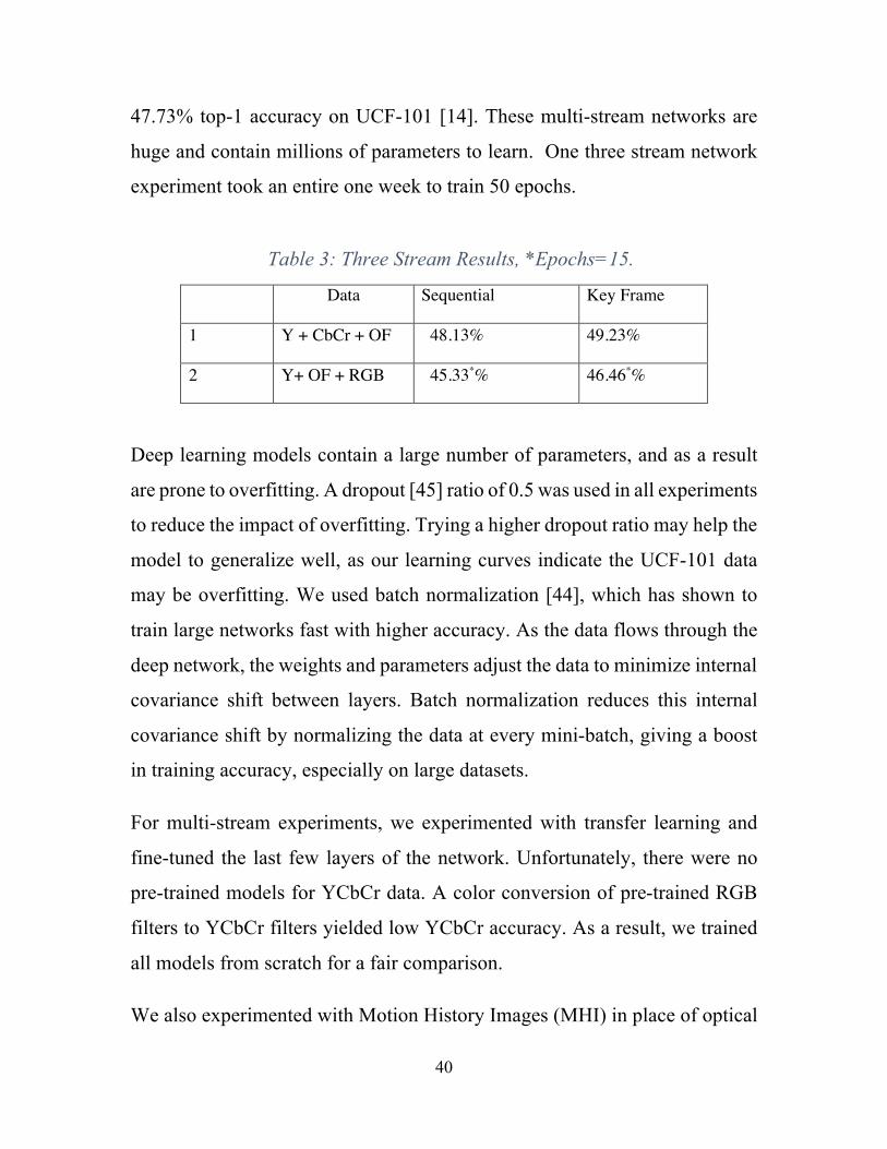
40

47.73% top-1 accuracy on UCF-101 [14]. These multi-stream networks are

huge and contain millions of parameters to learn. One three stream network

experiment took an entire one week to train 50 epochs.

Table 3: Three Stream Results, *Epochs=15.

Data Sequential Key Frame

1 Y + CbCr + OF 48.13% 49.23%

2 Y+ OF + RGB 45.33*% 46.46*%

Deep learning models contain a large number of parameters, and as a result

are prone to overfitting. A dropout [45] ratio of 0.5 was used in all experiments

to reduce the impact of overfitting. Trying a higher dropout ratio may help the

model to generalize well, as our learning curves indicate the UCF-101 data

may be overfitting. We used batch normalization [44], which has shown to

train large networks fast with higher accuracy. As the data flows through the

deep network, the weights and parameters adjust the data to minimize internal

covariance shift between layers. Batch normalization reduces this internal

covariance shift by normalizing the data at every mini-batch, giving a boost

in training accuracy, especially on large datasets.

For multi-stream experiments, we experimented with transfer learning and

fine-tuned the last few layers of the network. Unfortunately, there were no

pre-trained models for YCbCr data. A color conversion of pre-trained RGB

filters to YCbCr filters yielded low YCbCr accuracy. As a result, we trained

all models from scratch for a fair comparison.

We also experimented with Motion History Images (MHI) in place of optical

41

flow. A MHI template collapses motion information into a single gray scale

frame, where intensity of a pixel is directly related to recent pixel motion.

Single stream MHI resulted 26.7 % accuracy. This lower accuracy might be

improved by changing the fixed time parameter during the estimation of

motion images; we used ten frames to generate one motion image.

Our main goal was to experiment with different fusion techniques and key

frames, so we did not apply any data augmentation. All results in Tables 1

through III, except for the Y+OF+RGB, trained for 30 epochs so that we can

compare performance on the same scale. The Y+OF+RGB model was trained

for 15 epochs. We did observe the trend that running with higher number of

epochs increased the accuracy significantly. For example, the single stream

OF-only with key frames in Table 1 jumped to 57.8% after 117 epochs.

This work can be helpful with applications where speed is more important

than accuracy. In our experience, we saved computational time by a factor of

two and only used 60% of the entire UCF-101 dataset while keeping the

accuracy the same as the model trained on complete UCF-101 dataset. Current

state-of-the-art result [98] on UCF-101 is 93.1 % by taking advantage of very

deep hybrid convolutional neural networks. Such networks can take weeks to

optimize. Whereas our biggest CNN architecture took only four days of

learning time.

4.4.2 Filter Visualization

42

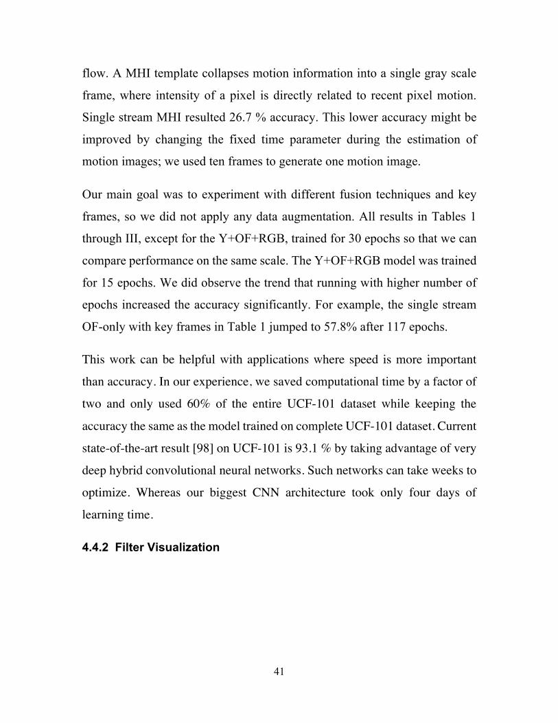
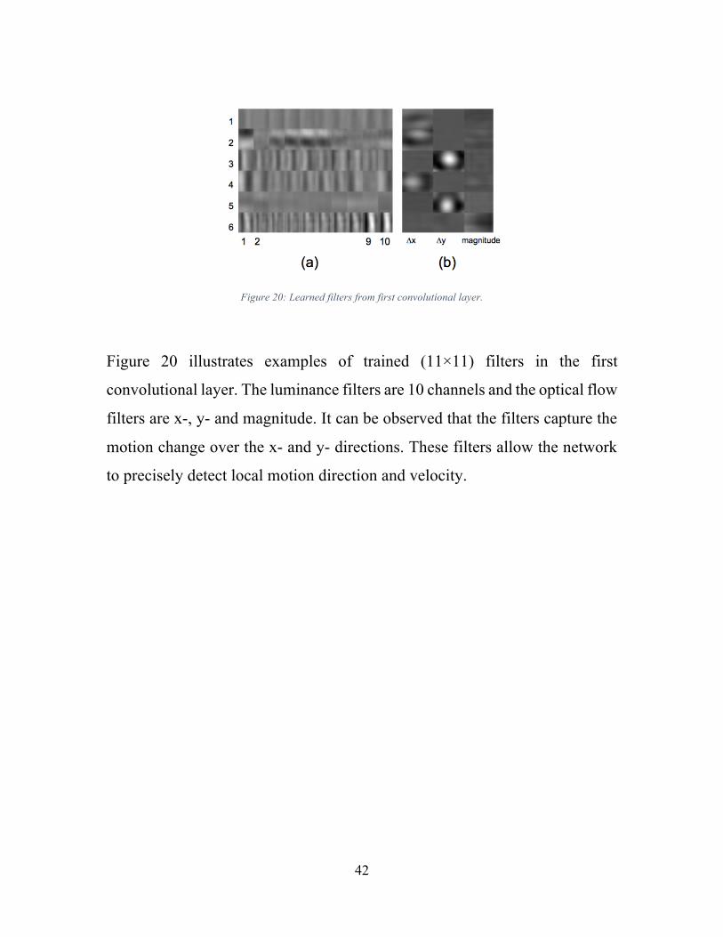
Figure 20: Learned filters from first convolutional layer.

Figure 20 illustrates examples of trained (11×11) filters in the first

convolutional layer. The luminance filters are 10 channels and the optical flow

filters are x-, y- and magnitude. It can be observed that the filters capture the

motion change over the x- and y- directions. These filters allow the network

to precisely detect local motion direction and velocity.

43

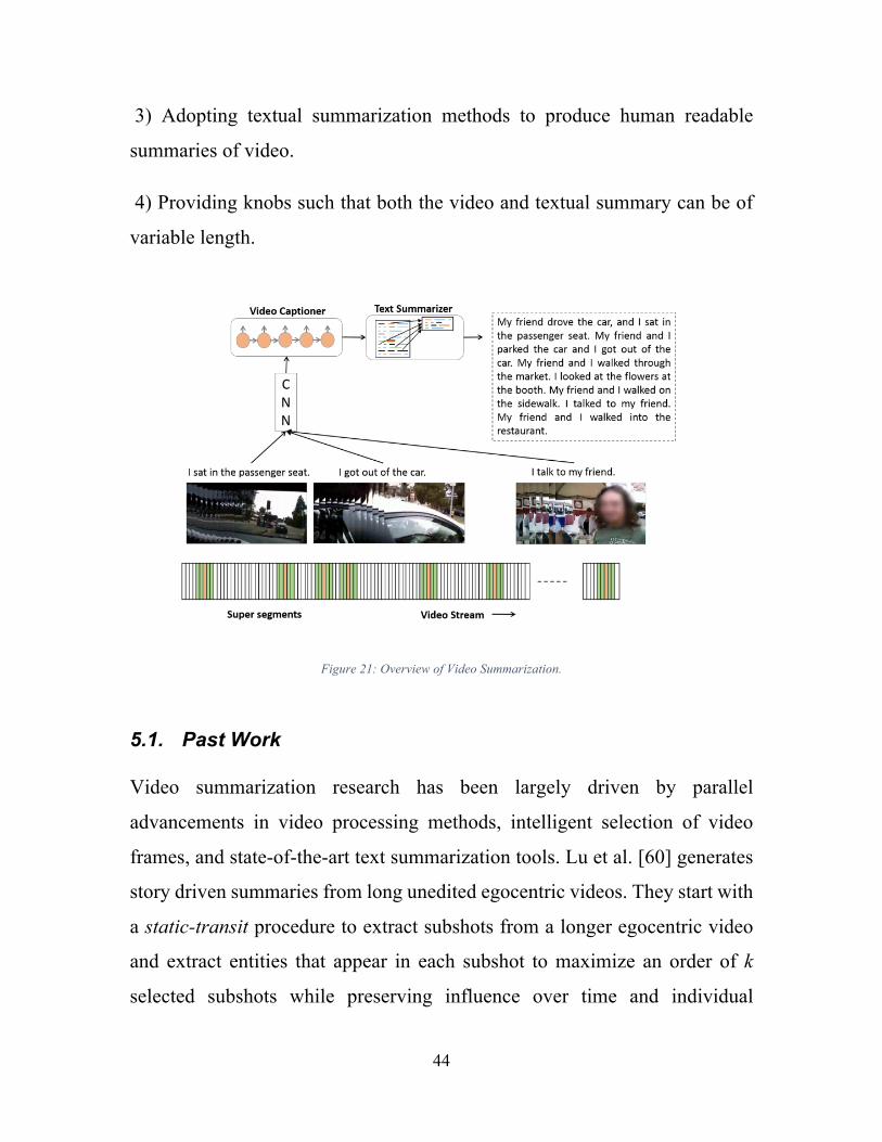
Chapter 5 Video Summarization Long videos captured by consumers are typically tied to some of the most

important moments of their lives, yet ironically are often the least frequently

watched. The time required to initially retrieve and watch sections can be

daunting. In this further work, we propose novel techniques for summarizing

and annotating long videos. Existing video summarization techniques focus

exclusively on identifying keyframes and subshots, however evaluating these

summarized videos is a challenging task. Our work proposes methods to

generate visual summaries of long videos, and in addition proposes techniques

to annotate and generate textual summaries of the videos using recurrent

neural networks. Interesting segments of long video are extracted based on

image quality as well as cinematographic and consumer preference. Key

frames from the most impactful segments are converted to textual annotations

using sequential encoding and decoding deep learning models. Our

summarization technique as shown in Figure 21 is benchmarked on the

VideoSet dataset, and evaluated by humans for informative and linguistic

content. We believe this to be the first fully automatic method capable of

simultaneous visual and textual summarization of long consumer videos. The

novel contributions of this work include:

1) The ability to split a video into superframe segments, ranking each segment

by image quality, cinematography rules, and consumer preference.

2) Advancing the field of video annotation by combining recent deep learning

discoveries in image classification, recurrent neural networks, and transfer

learning.

44

3) Adopting textual summarization methods to produce human readable

summaries of video.

4) Providing knobs such that both the video and textual summary can be of

variable length.

Figure 21: Overview of Video Summarization.

5.1. Past Work Video summarization research has been largely driven by parallel

advancements in video processing methods, intelligent selection of video

frames, and state-of-the-art text summarization tools. Lu et al. [60] generates

story driven summaries from long unedited egocentric videos. They start with

a static-transit procedure to extract subshots from a longer egocentric video

and extract entities that appear in each subshot to maximize an order of k

selected subshots while preserving influence over time and individual

45

important events. In contrast, Gygli et al. [61] works with any kind of video

(static, egocentric or moving), generates superframe cuts based on motion and

further estimates interestingness of each superframe based on attention,

aesthetic quality, landmark, person and objects. They select an optimal set of

such superframes to generate an interesting video summary. Song et al. [62]

uses video titles to find most important video segments. Their framework

search for visually important shots uses at title-based image search. It takes

advantage of the fact that video titles are highly descriptive of video content

and therefore serve as a good proxy for relevant visual video content. Zhang

et al. [47] explores a nonparametric supervised learning approach for

summarization and transfers summary structure to novel input videos. Their

method can be used in a semi-supervised way to comprehend semantic

information about visual content of the video. Determinantal Point Process

has also often been used in video summary methods [62, 63, 47].

Using key frames to identify important or interesting regions of video has

proven to be a valuable first step in video summarization. For example, Ejaz

et al. [16] used temporal motion to define a visual attention score. Similarly,

Hou et al. [15] utilized spatial saliency at the frame level. Gygli et al. [61]

introduced cinematographic rules which pull segment boundaries to locations

with minimum motion. KE et al. [65] favored frames with higher contrast and

sharpness, Datta et at. [66] favored more colorful frames, Ghosh et al. [67]

studied people and object content, while Ptucha et al. [68] studied the role

facial content plays in image preference. [67] further tracked objects across a

long video to discover story content.

Large supervised datasets along with advances in recurrent deep networks

have enabled realistic description of still images with natural language text

46

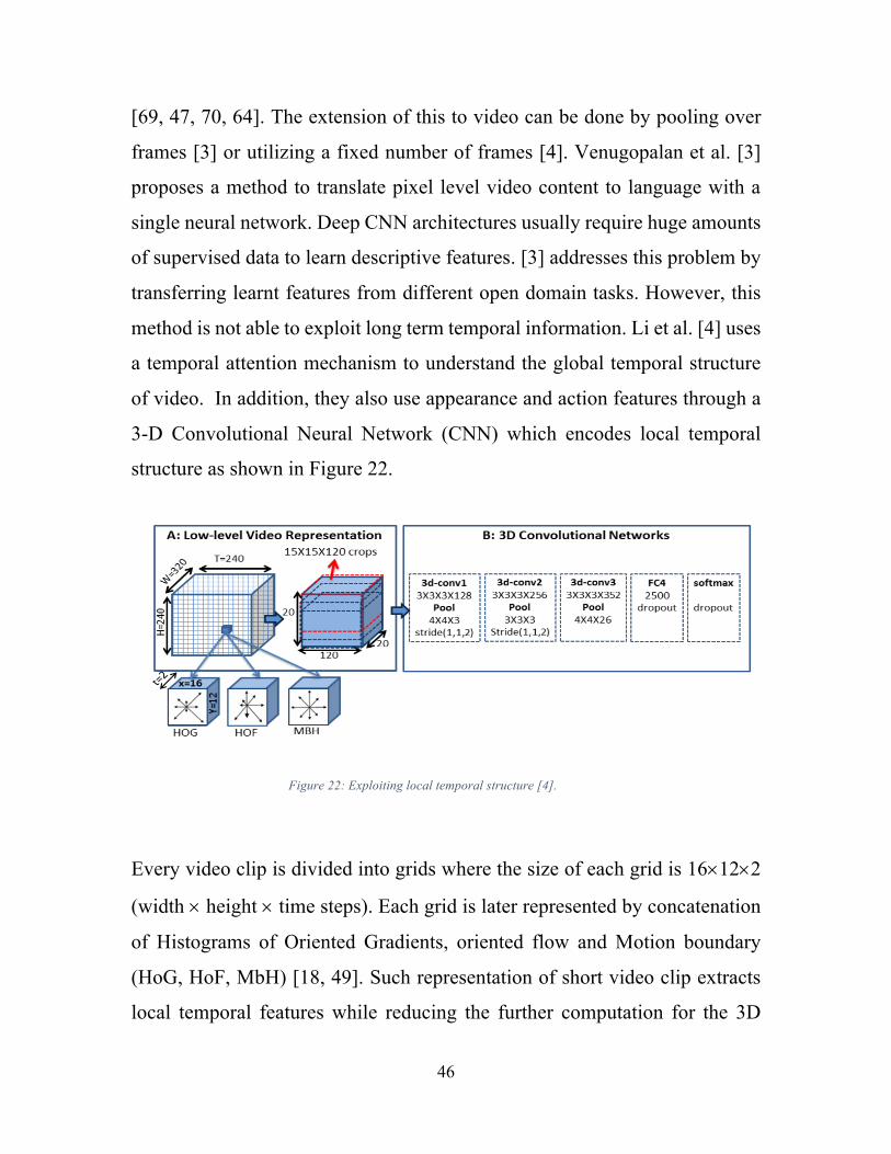
[69, 47, 70, 64]. The extension of this to video can be done by pooling over

frames [3] or utilizing a fixed number of frames [4]. Venugopalan et al. [3]

proposes a method to translate pixel level video content to language with a

single neural network. Deep CNN architectures usually require huge amounts

of supervised data to learn descriptive features. [3] addresses this problem by

transferring learnt features from different open domain tasks. However, this

method is not able to exploit long term temporal information. Li et al. [4] uses

a temporal attention mechanism to understand the global temporal structure

of video. In addition, they also use appearance and action features through a

3-D Convolutional Neural Network (CNN) which encodes local temporal

structure as shown in Figure 22.

Figure 22: Exploiting local temporal structure [4].

Every video clip is divided into grids where the size of each grid is 16´12´2

(width ´ height ´ time steps). Each grid is later represented by concatenation

of Histograms of Oriented Gradients, oriented flow and Motion boundary

(HoG, HoF, MbH) [18, 49]. Such representation of short video clip extracts

local temporal features while reducing the further computation for the 3D

47

CNN.

Most recently, Venugopalan et al. [11] described a technique, S2VT, to learn

a representation of a variable sequence of frames which are decoded into

natural text. Recently, Yu et al. [71] demonstrated a hierarchical recurrent

neural network to generate paragraph summaries from relatively long videos.

These videos were still limited to a few minutes long. We use a variation of

the S2VT captioning approach in our work.

Given descriptive captions at key frame locations, we explore extractive

methods for summarization. Extractive methods analyze a collection of input

text to be summarized, typically sentences. These sentences are selected to be

included in the summary using various measurements of sentence importance

or centrality. Early seminal summarization research by Luhn [72] used word

frequency metrics to rank sentences for inclusion in summaries, while

Edmundson [73] expanded this approach to include heuristics based on word

position in a sentence, sentence position in a document, and the presence of

nearby key phrases. More recent extensions of the word frequency models,

including SumBasic [74] and KL-Sum [75], typically incorporate more

sophisticated methods of combining measures of word frequency at the

sentence level and using these composite measures to rank candidate

sentences. Other approaches, such as LexRank [76] and TextRank [77] focus

on centroid-based methods of sentence selection, in which random walks on

graphs of words and sentences are used to measure the centrality of those

sentences to the text being summarized. A good review of these techniques

and others can be found in [78, 79]. The latest research on single document

summarization has utilized both dependency based discourse tree trimming

[80] as well as compression and anaphoricity constraints [81].

48

Natural language summarization can be classified into two types of methods:

extractive summarization and abstractive summarization. Extractive

summarization involves giving confident scores to each sentence/group of

sentences and determine the importance of each sentence/group of sentences

in the given text and later concatenate these filtered parts of given text to form

a shorter version. The importance of individual parts is driven by statistical

and linguistic features present in each part. In contrast, abstractive

summarization [88] tries to understand the main centralities in the document

and constitutes the sentences that convey the main context while preserving

the amount of necessary information being expressed. In this work, we prove

that abstractive summarization methods are well suited for video

summarization.

5.2. Methodology Our proposed approach consists of four main components:

• Identification of interesting segments from the full video;

• Key frame extraction from these interesting segments;

• Annotation generation of key frames using a deep video-captioning

network;

• Annotation summarization to generate a paragraph description of the

sequence of events in the video.

The annotations from the key frames form powerful search descriptors, both

for finding the appropriate video, and for quickly jumping to the appropriate

frame location in the video. The selected interesting segments form a visual

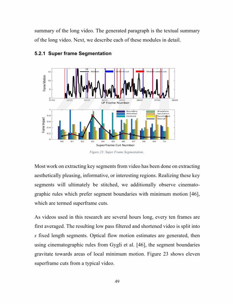
49

summary of the long video. The generated paragraph is the textual summary

of the long video. Next, we describe each of these modules in detail.

5.2.1 Super frame Segmentation

Figure 23: Super Frame Segmentation.

Most work on extracting key segments from video has been done on extracting

aesthetically pleasing, informative, or interesting regions. Realizing these key

segments will ultimately be stitched, we additionally observe cinemato-

graphic rules which prefer segment boundaries with minimum motion [46],

which are termed superframe cuts.

As videos used in this research are several hours long, every ten frames are

first averaged. The resulting low pass filtered and shortened video is split into

s fixed length segments. Optical flow motion estimates are generated, then

using cinematographic rules from Gygli et al. [46], the segment boundaries

gravitate towards areas of local minimum motion. Figure 23 shows eleven

superframe cuts from a typical video.

50

Given s superframe cuts, we need to decide which are worthy of inclusion in

the final summary, and which will be edited out. Worthiness will be

determined by a non-linear combination of scores measuring a superframe

cut’s fitness regarding Boundary, Attention, Contrast, Sharpness, Saturation,

and Facial impact. Each of these will be described next.

5.2.1.1 Boundary Score

A Boundary score, B is computed for each superframe region, where the score

is inversely proportional to the motion at each boundary neighborhood.

Similar to Zhang et al. [64], we stack the optical flow between consecutive

frames in the x- and y- directions. Motion is computed as M 𝒕 (see key frame

selection 4.3.4), then given:

M 𝑡 , B = 1/ M 𝑡 (5.1)

5.2.1.2 Attention Score

Each of these superframe regions are evaluated for aesthetic and interesting

properties. Similar to [16, 15], an Attention score, based on temporal saliency

is first used. The Attention score, A is a combination of the super-frame

motion, m and variance, v, where m and v correspond to the mean and

variance of all non-boundary frames motion in a superframe cut. The final

Attention score:

A = α ∗ m + (1 − α) ∗ v, with α = 0.7 (5.2)

51

5.2.1.3 Contrast Score

The measures of Contrast, Sharpness, Saturation, and Facial impact are

computed for all frames in each super-frame cut and then averaged to report

four values for each superframe cut. Similar to Ke et al. [65], a Contrast score

is com- puted. To calculate the Contrast score, C, each frame in a superframe

cut is converted to luminance, low pass filtered, and resampled to 64 × width,

where 64 is the new height and width is selected to preserve the aspect ratio

of the frame. The Contrast score, C, is the standard deviation of luminance

pixels.

5.2.1.4 Sharpness Score

Similar to Ke et al. [65], a Sharpness score is computed. To calculate a

Sharpness score, E, the frames are converted to luminance, then divided up

into 10 × 10 equally spaced regions. Using the center 7 × 7 regions, the

standard deviation of luminance pixels is calculated three times centered on

each region, where each of the three times a random shift is added, and the

median of the three standard deviation values is reported for each of the 49

regions. The Sharpness score, E is the maximum of the 49 standard deviation

values.

5.2.1.5 Colorfulness Score

Similar to Datta et al. [66], a Colorfulness score, S is computed. The frames

are converted to HSV space, low pass filtered, resampled to 64 × width, where

64 is the new height and width is selected to preserve the aspect ratio of the

frame, then the mean saturation value from the frame is reported.

52

5.2.1.6 Facial Impact Score Ptucha et al. [68] reported on the importance of facial content in imagery,

and described a method for generating aesthetically pleasing crops of images

containing facial information. Similar to Gygli et al. [46], but following the

rules from [68], we compute a Face impact score, F which favors larger and

more centrally located faces. Each face is assigned an impact score and the

sum of all face scores is reported as a Face impact score, F. To convert from

pixels to a universal unit of measure, the size of a face, FS is normalized to

the size of the image using:

𝐹𝑆 =

𝑓𝑎𝑐𝑒𝑊𝑖𝑑𝑡ℎC

𝑖𝑚𝑎𝑔𝑒𝑊𝑖𝑑𝑡ℎ×𝑖𝑚𝑎𝑔𝑒𝐻𝑒𝑖𝑔ℎ𝑡 (5.3)

where faceWidth is the width of the face bounding box in pixels, or 2 ×

intraocular distance if bounding boxes are not square. Finally, following [68],

the face size attribute, FSA is normalized to 0:1, centered on 0.5 for a typical

face:

𝐹𝑆𝐴 = −72.4 ∗ 𝐹𝑆M + 27.2 ∗ 𝐹𝑆C − 0.26 ∗ 𝐹𝑆 + 0.5 (5.4)

5.2.1.7 Fusing Scores

Empirical testing has shown that Attention (A), Contrast (C), and Sharpness

(E) are essential elements to the usefulness and fidelity of a superframe region.

After normalization, the product of these three scores is used to form a

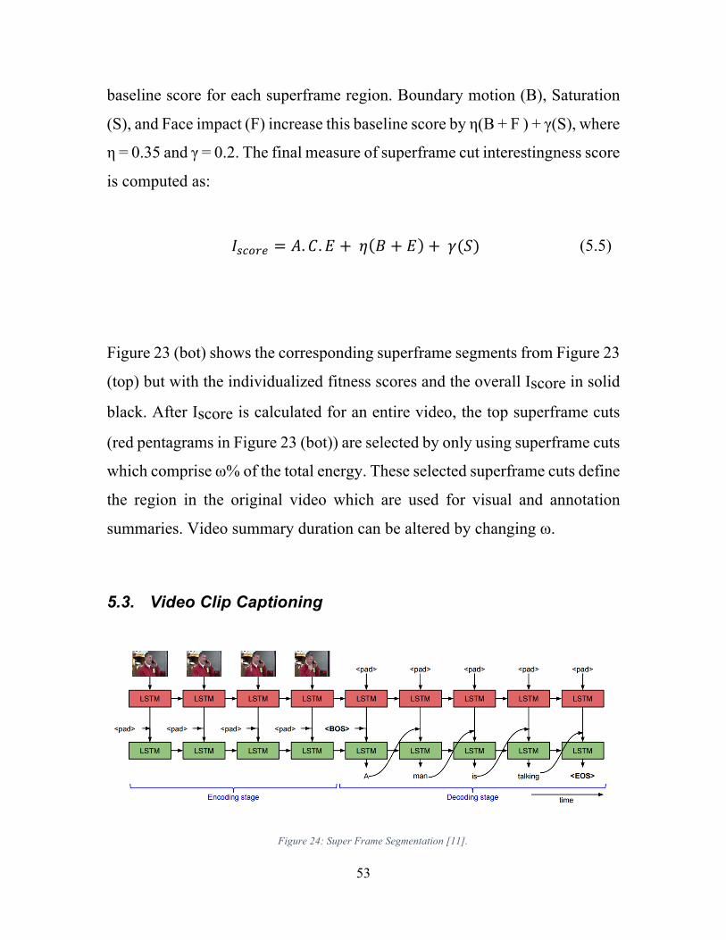
53

baseline score for each superframe region. Boundary motion (B), Saturation

(S), and Face impact (F) increase this baseline score by η(B + F ) + γ(S), where

η = 0.35 and γ = 0.2. The final measure of superframe cut interestingness score

is computed as:

𝐼RSTUV = 𝐴. 𝐶. 𝐸 + 𝜂 𝐵 + 𝐸 + 𝛾(𝑆) (5.5)

Figure 23 (bot) shows the corresponding superframe segments from Figure 23

(top) but with the individualized fitness scores and the overall Iscore in solid

black. After Iscore is calculated for an entire video, the top superframe cuts

(red pentagrams in Figure 23 (bot)) are selected by only using superframe cuts

which comprise ω% of the total energy. These selected superframe cuts define

the region in the original video which are used for visual and annotation

summaries. Video summary duration can be altered by changing ω.

5.3. Video Clip Captioning

Figure 24: Super Frame Segmentation [11].

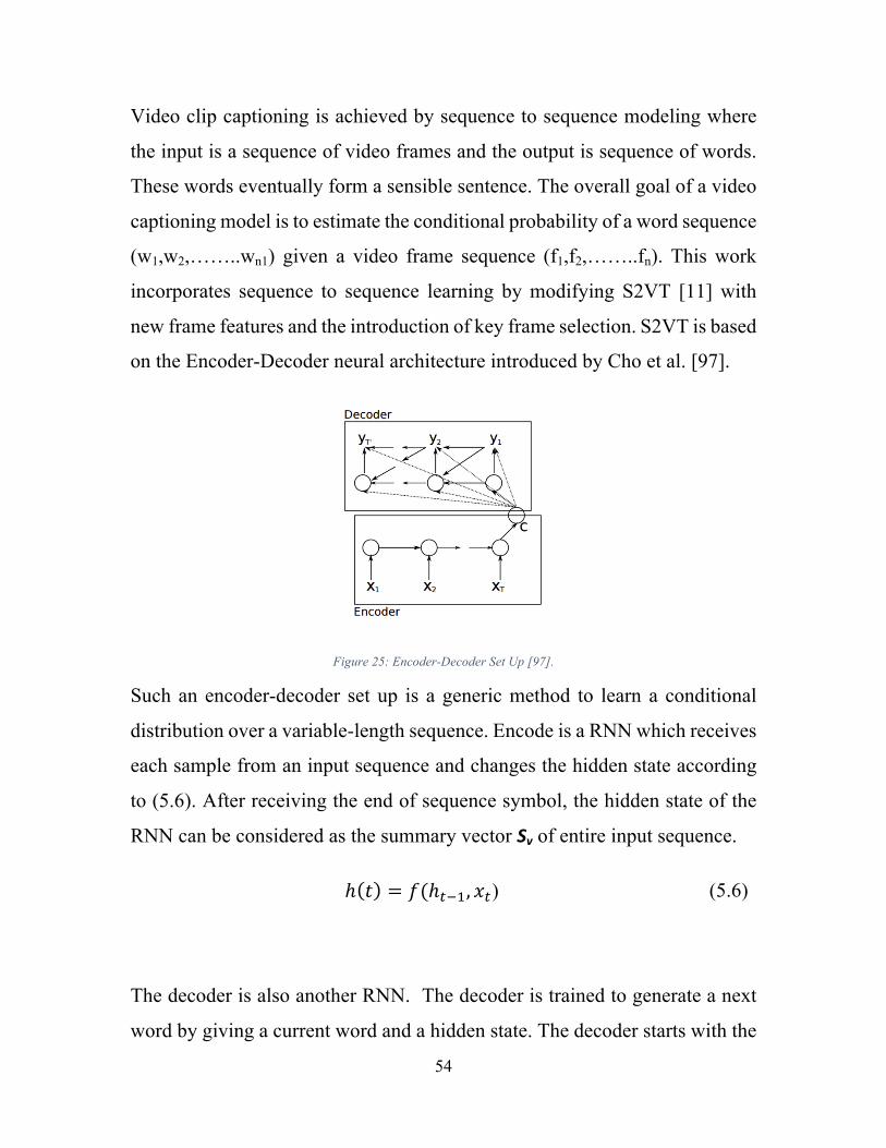
54

Video clip captioning is achieved by sequence to sequence modeling where

the input is a sequence of video frames and the output is sequence of words.

These words eventually form a sensible sentence. The overall goal of a video

captioning model is to estimate the conditional probability of a word sequence

(w1,w2,……..wn1) given a video frame sequence (f1,f2,……..fn). This work

incorporates sequence to sequence learning by modifying S2VT [11] with

new frame features and the introduction of key frame selection. S2VT is based

on the Encoder-Decoder neural architecture introduced by Cho et al. [97].

Figure 25: Encoder-Decoder Set Up [97].

Such an encoder-decoder set up is a generic method to learn a conditional

distribution over a variable-length sequence. Encode is a RNN which receives

each sample from an input sequence and changes the hidden state according

to (5.6). After receiving the end of sequence symbol, the hidden state of the

RNN can be considered as the summary vector Sv of entire input sequence.

ℎ 𝑡 = 𝑓(ℎ\],, 𝑥\) (5.6)

The decoder is also another RNN. The decoder is trained to generate a next

word by giving a current word and a hidden state. The decoder starts with the

55

summary hidden state from the encoder and a start token. Unlike the encoder,

the hidden state of the decoder depends not only on the input and hidden state,

but also the summary vector Sv as depicted in (5.7):

ℎ 𝑡 = 𝑓(ℎ\],, 𝑦\],, 𝑆`), (5.7)

Further, the conditional distribution of next sample in sequence can be

expressed as:

𝑃 𝑦\ 𝑦\],, 𝑦\]C, 𝑦\]M, . . . . . . , 𝑦,, 𝑐 = 𝑔(ℎ\, 𝑦\],, 𝑐) (5.8)

Where g is the activation function.

S2VT is shown in Figure 24. Each key frame is passed through the 152-layer

ResNet CNN model [82] pre-trained on ImageNet data, where the [1 × 2048]

vector from the last pooling layer is used as a frame feature. These key frame

feature vectors are passed sequentially into a LSTM network [83].

The S2VT framework first encodes (similar to encode-decoder) fframes, one

frame at a time to the first layer of a two-layer LSTM, where f is of variable

length. This latent representation is then decoded into a natural language

sentence one word at a time, feeding the output of one time step into the

second layer of the LSTM in the subsequent time step as shown in Figure 24.

During training, a video sequence and corresponding text annotation pair are

input to the network. During testing, f key frames around a superframe video

segment are encoded into the trained neural network. Once all frames are

56

processed, a begin of sentence keyword is fed into the network, triggering

word generation until and end of sentence keyword is produced. The two layer

LSTM is fixed to 80 time steps, which includes both the input frames for each

clip as well as its associated caption.

Our code base is available on RIT gitlab server with the use of following link:

git@kgcoe-git.rit.edu:sk1846/video_captioning.git. It includes Torch7 based

Lua scripts to extract CNN ResNet/GoogLeNet features. It also comprises

summary evaluation scripts.

5.4. Text Summarization After passing the extracted video clips through a video captioning model, a

list of sentences is returned which describes the information flow in the

original video. These sentences still show some redundant information,

creating the need for an abstractive/narrative summary which can convey the

overview of video information in a condensed form. This work explores

various methods to perform this summarization task. Text summarization can

be categorized into two types, extractive summarization and abstractive

summarization. Extractive summarization strictly generates summary based

on the input text given. It can be thought as giving importance to some parts

of text based on natural language features and stitching them together to form

a summary. Whereas, abstractive summarization is a transformation process;

input text is transformed into summary through data driven statistical models.

5.4.1 Extractive Summarization The sumy 0.4.1 python framework along with NLTK libraries were used to

evaluate Luhn’s algorithm, Edmundson’s heuristic method, Latent Semantic

Analysis (LSA), LexRank, TextRank, SumBasic and KL-Sum text summa-

57

rization techniques. Before passing video clip captions into the text

summarizers, duplicate captions were filtered out. The temporal order of each

caption was preserved, and the summary length was fixed to 24 sentences for

this paper, but can be changed to any length greater than the number of input

captions.

5.4.2 Abstractive Summarization This work improves video to text summarization by using abstractive

summarization techniques through a contextual attention encoder with neural

network language model. Attention based summarization is the core concept

of this approach. It incorporates little to no information about language

templates and other linguistic rules. It is completely data driven. Although it

requires a huge amount of document-summary data to learn, the results

generated by attention based summarization techniques often outperform

extractive summarization methods.

This approach, inspired by Rush et al. [89], involves joint learning of a

language model and a contextual input encoder. The contextual encoder is the

extension of Bahdanau et al. [90]. Such an encoder arrangement can learn a

latent soft alignment between input text and generated summary. The goal of

a document summarization method is: given an input text x, which is a

sequence of M words, generate a condensed summary y which contains N

words. In this problem, N is significantly smaller than M, which drives the

condensed summarization. Both input and output sequences share a common

vocabulary V of size V. Abstractive summarization methods use a scoring

function (5.9) to form an optimal sequence of N words.

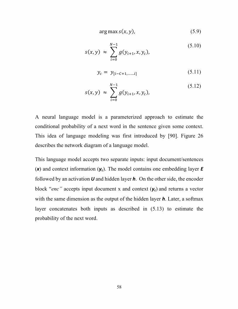
58

argmax 𝑠 𝑥, 𝑦 , (5.9)

𝑠 𝑥, 𝑦 ≈ 𝑔 𝑦hi,, 𝑥, 𝑦S

j],

hkl

, (5.10)

𝑦S = 𝑦[h]ni,,…….h] (5.11)

𝑠 𝑥, 𝑦 ≈ 𝑔 𝑦hi,, 𝑥, 𝑦S

j],

hkl

,

(5.12)

A neural language model is a parameterized approach to estimate the

conditional probability of a next word in the sentence given some context.

This idea of language modeling was first introduced by [90]. Figure 26

describes the network diagram of a language model.

This language model accepts two separate inputs: input document/sentences

(x) and context information (yc). The model contains one embedding layer E

followed by an activation U and hidden layer h. On the other side, the encoder

block “enc” accepts input document x and context (yc) and returns a vector

with the same dimension as the output of the hidden layer h. Later, a softmax

layer concatenates both inputs as described in (5.13) to estimate the

probability of the next word.

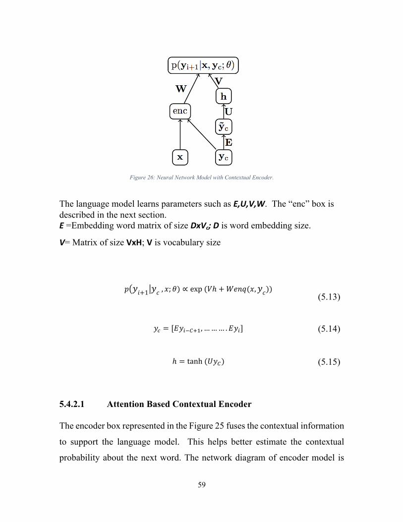
59

Figure 26: Neural Network Model with Contextual Encoder.

The language model learns parameters such as E,U,V,W. The “enc” box is described in the next section. E =Embedding word matrix of size DxVc;D is word embedding size.

V= Matrix of size VxH; V is vocabulary size

𝑝 𝑦𝑖+1 𝑦𝑐, 𝑥; 𝜃) ∝ exp(𝑉ℎ +𝑊𝑒𝑛𝑞(𝑥, 𝑦𝑐))

(5.13)

𝑦S = [𝐸𝑦h]ni,, ……… . 𝐸𝑦h]

(5.14)

ℎ = tanh(𝑈𝑦n)

(5.15)

5.4.2.1 Attention Based Contextual Encoder The encoder box represented in the Figure 25 fuses the contextual information

to support the language model. This helps better estimate the contextual

probability about the next word. The network diagram of encoder model is

60

shown in the Figure 27, where F is input side embedding matrix of size (DxV)

G is context side embedding matrix with similar size, P is a weight matrix

which maps parameters between the context embedding and input embedding,

and Q is the smoothing window on the input sequences.

Figure 27: Neural Language Model with contextual encoder.

𝑒𝑛𝑐 𝑥, 𝑦S = 𝑃¢𝑥 (5.16)

𝑃µexp(𝑥]𝑃𝑦S{) (5.17)

𝑥] = [𝐹𝑥,, 𝐹𝑥C …… . . 𝐹𝑥|]

(5.18)

𝑦S{ = [𝐺𝑦h]ni,, …… . . 𝐺𝑦h]

(5.19)

𝑥h] = 𝑥h~/𝑄

hi�

�kh]�

(5.20)

61

One way to think about the encoder model as a normal avererager is if Yc is

not present in (5.17). The inclusion of Yc works as soft alignment between the

input sequence and the generated sequence. During the learning process, such

alignment tries to align context words with the input sequence. Working

software can be accessed through RIT gitlab server with the following link

https://kgcoe-git.rit.edu/sk1846/sentence_modeling. It includes the following

scripts:

1. Construct_data.sh : Neural attention model accepts text into a certain

format, this script converts a text document into a sequence of numbers

where each number correspond to vocabulary index.

2. Train_model.sh : This calls train.lua script with the given flags. Short

description of each flag is present in the train.lua script.

5.4.3 Summarization Metric: Rouge-2 In order to evaluate the summaries produced in this way, we turned to ROUGE

[84], a set of objective metrics of summarization quality that can be calculated

automatically, making them ideal for development and comparison of

summaries generated by multiple summarization models. These metrics rely

on methods of measuring word overlap between the output of a summarization

system and one or more human generated reference summaries. Although

simple, the ROUGE metrics correlate very highly with human evaluations.

Here we use ROUGE-2, which measures the number of bigrams (i.e., two-

word sequences) appearing in the summarization output that also appear in

the reference summaries. ROUGE-2 is one of the more commonly used

variation of the ROUGE metric in the text summarization research community

and is the variant of ROUGE-N with the highest correlation with human

evaluation. Using Lin’s notation, ROUGE-2 is formulated as follows: where

62

Refs is the set of reference summaries, Count(bigram) is the count of a

bigram, and Countmatch(bigram) is the number of matching bigrams in the

summarization output:

𝑅𝑂𝑈𝐺𝐸2 = 𝐶𝑜𝑢𝑛𝑡��\S�(𝑏𝑖𝑔𝑟𝑎𝑚)�h�U��∈��∈�V�R

𝐶𝑜𝑢𝑛𝑡(𝑏𝑖𝑔𝑟𝑎𝑚)�h�U��∈��∈�V�R (5.21)

Our purpose is to quantify abstractive summarization. ROUGE-2 is the best

acceptable metric but it captures only bi-gram overlaps between model output

summary and the gold summary. Abstractive summarization often rephrases

the sentence or uses different sets of words, which provides understandable

summary. ROUGE-2 often underrates the summary because it doesn’t find

exact word pairs. In the linguistic community, there is strong need to have an

adequate metric to measure abstractive summarization quality.

BLEU and METEOR scores are familiar techniques for machine translation

quality measurement. BLEU scores scale between 0 to 1- a score near 1 is

considered highly correlated with human translation. BLEU evaluates a

generated summary based on the similarity of n-grams with a reference

summary. METEOR evaluates machine translation by aligning output

summary words with reference summary words, where alignment is based on

exact match, synonym, or paraphrase.

In the case of abstractive summarization, the model paraphrases multiple

sentences into few sentences which involves words elimination, change in

sentence structure, synonym addition and other possible language changes. It

is common understanding that none of the scoring methods (ROUGE-2,

BLEU, METEOR) are alone capable to sense all kinds of natural language

issues in the process of abstractive summarization.

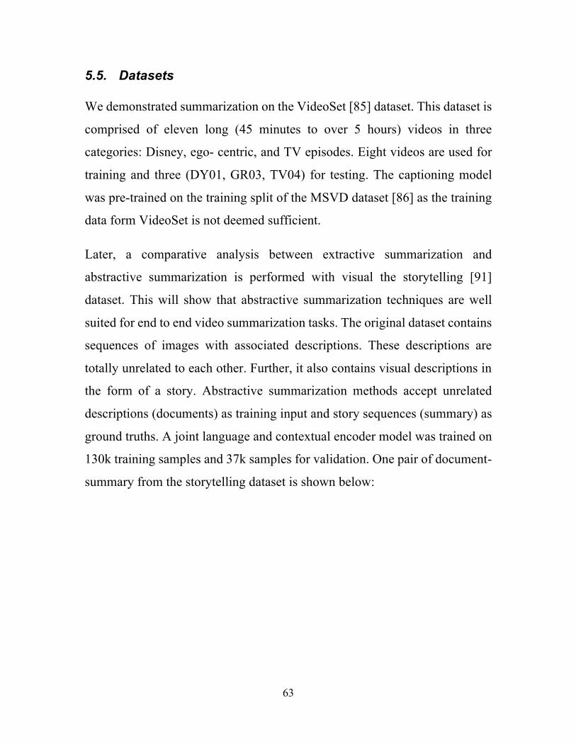
63

5.5. Datasets We demonstrated summarization on the VideoSet [85] dataset. This dataset is

comprised of eleven long (45 minutes to over 5 hours) videos in three

categories: Disney, ego- centric, and TV episodes. Eight videos are used for

training and three (DY01, GR03, TV04) for testing. The captioning model

was pre-trained on the training split of the MSVD dataset [86] as the training

data form VideoSet is not deemed sufficient.

Later, a comparative analysis between extractive summarization and

abstractive summarization is performed with visual the storytelling [91]

dataset. This will show that abstractive summarization techniques are well

suited for end to end video summarization tasks. The original dataset contains

sequences of images with associated descriptions. These descriptions are

totally unrelated to each other. Further, it also contains visual descriptions in

the form of a story. Abstractive summarization methods accept unrelated

descriptions (documents) as training input and story sequences (summary) as

ground truths. A joint language and contextual encoder model was trained on

130k training samples and 37k samples for validation. One pair of document-

summary from the storytelling dataset is shown below:

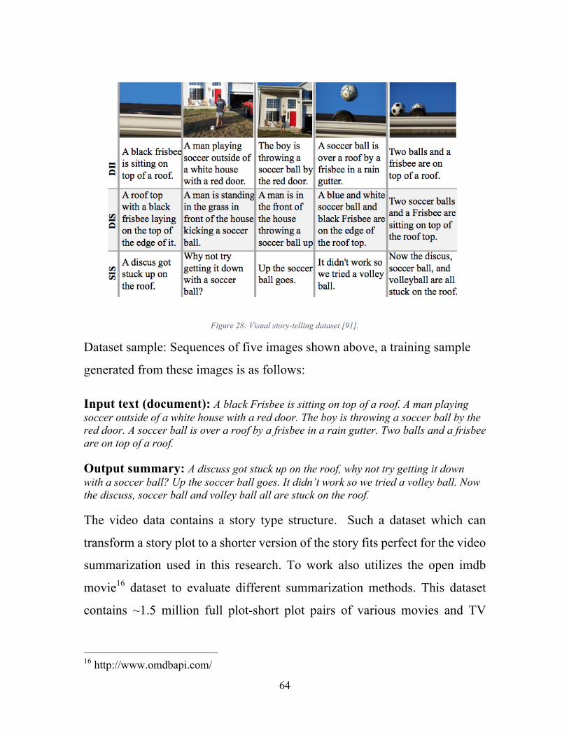
64

Figure 28: Visual story-telling dataset [91].

Dataset sample: Sequences of five images shown above, a training sample

generated from these images is as follows:

Input text (document): A black Frisbee is sitting on top of a roof. A man playing soccer outside of a white house with a red door. The boy is throwing a soccer ball by the red door. A soccer ball is over a roof by a frisbee in a rain gutter. Two balls and a frisbee are on top of a roof.

Output summary: A discuss got stuck up on the roof, why not try getting it down with a soccer ball? Up the soccer ball goes. It didn’t work so we tried a volley ball. Now the discuss, soccer ball and volley ball all are stuck on the roof.

The video data contains a story type structure. Such a dataset which can

transform a story plot to a shorter version of the story fits perfect for the video

summarization used in this research. To work also utilizes the open imdb

movie16 dataset to evaluate different summarization methods. This dataset

contains ~1.5 million full plot-short plot pairs of various movies and TV

16 http://www.omdbapi.com/

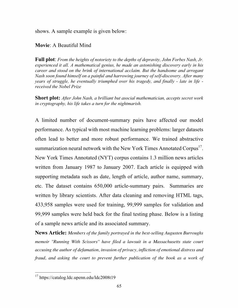
65

shows. A sample example is given below:

Movie: A Beautiful Mind

Full plot: From the heights of notoriety to the depths of depravity, John Forbes Nash, Jr. experienced it all. A mathematical genius, he made an astonishing discovery early in his career and stood on the brink of international acclaim. But the handsome and arrogant Nash soon found himself on a painful and harrowing journey of self-discovery. After many years of struggle, he eventually triumphed over his tragedy, and finally - late in life - received the Nobel Prize Short plot: After John Nash, a brilliant but asocial mathematician, accepts secret work in cryptography, his life takes a turn for the nightmarish. A limited number of document-summary pairs have affected our model

performance. As typical with most machine learning problems: larger datasets

often lead to better and more robust performance. We trained abstractive

summarization neural network with the New York Times Annotated Corpus17.

New York Times Annotated (NYT) corpus contains 1.3 million news articles

written from January 1987 to January 2007. Each article is equipped with

supporting metadata such as date, length of article, author name, summary,

etc. The dataset contains 650,000 article-summary pairs. Summaries are

written by library scientists. After data cleaning and removing HTML tags,

433,958 samples were used for training, 99,999 samples for validation and

99,999 samples were held back for the final testing phase. Below is a listing

of a sample news article and its associated summary.

News Article: Members of the family portrayed in the best-selling Augusten Burroughs

memoir ''Running With Scissors'' have filed a lawsuit in a Massachusetts state court

accusing the author of defamation, invasion of privacy, infliction of emotional distress and

fraud, and asking the court to prevent further publication of the book as a work of

17 https://catalog.ldc.upenn.edu/ldc2008t19

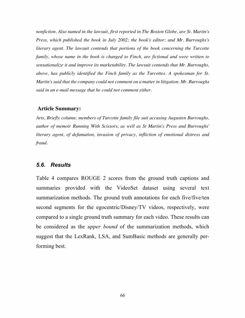
66

nonfiction. Also named in the lawsuit, first reported in The Boston Globe, are St. Martin's

Press, which published the book in July 2002; the book's editor; and Mr. Burroughs's

literary agent. The lawsuit contends that portions of the book concerning the Turcotte

family, whose name in the book is changed to Finch, are fictional and were written to

sensationalize it and improve its marketability. The lawsuit contends that Mr. Burroughs,

above, has publicly identified the Finch family as the Turcottes. A spokesman for St.

Martin's said that the company could not comment on a matter in litigation. Mr. Burroughs

said in an e-mail message that he could not comment either.

Article Summary: Arts, Briefly column; members of Turcotte family file suit accusing Augusten Burroughs,

author of memoir Running With Scissors, as well as St Martin's Press and Burroughs'

literary agent, of defamation, invasion of privacy, infliction of emotional distress and

fraud.

5.6. Results Table 4 compares ROUGE 2 scores from the ground truth captions and

summaries provided with the VideoSet dataset using several text

summarization methods. The ground truth annotations for each five/five/ten

second segments for the egocentric/Disney/TV videos, respectively, were

compared to a single ground truth summary for each video. These results can

be considered as the upper bound of the summarization methods, which

suggest that the LexRank, LSA, and SumBasic methods are generally per-

forming best.

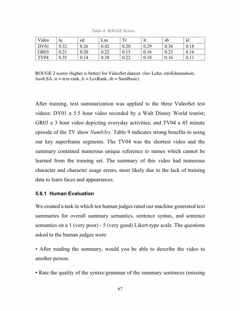
67

Table 4: ROUGE Scores.

Video lu ed Lsa Tr lr sb kl DY01 0.32 0.26 0.42 0.20 0.29 0.36 0.18 GR03 0.21 0.20 0.22 0.15 0.16 0.23 0.16 TV04 0.35 0.14 0.38 0.22 0.18 0.16 0.11

ROUGE 2 scores (higher is better) for VideoSet dataset. (lu= Luhn, ed=Edmundson, lsa=LSA, tr = text-rank, lr = LexRank, sb = SumBasic)

After training, text summarization was applied to the three VideoSet test

videos: DY01 a 5.5 hour video recorded by a Walt Disney World tourist;

GR03 a 3 hour video depicting everyday activities; and TV04 a 45 minute

episode of the TV show Numb3rs. Table 9 indicates strong benefits to using

our key superframe segments. The TV04 was the shortest video and the

summary contained numerous unique reference to names which cannot be

learned from the training set. The summary of this video had numerous

character and character usage errors, most likely due to the lack of training

data to learn faces and appearances.

5.6.1 Human Evaluation We created a task in which ten human judges rated our machine generated text

summaries for overall summary semantics, sentence syntax, and sentence

semantics on a 1 (very poor) - 5 (very good) Likert-type scale. The questions

asked to the human judges were:

• After reading the summary, would you be able to describe the video to

another person.

• Rate the quality of the syntax/grammar of the summary sentences (missing

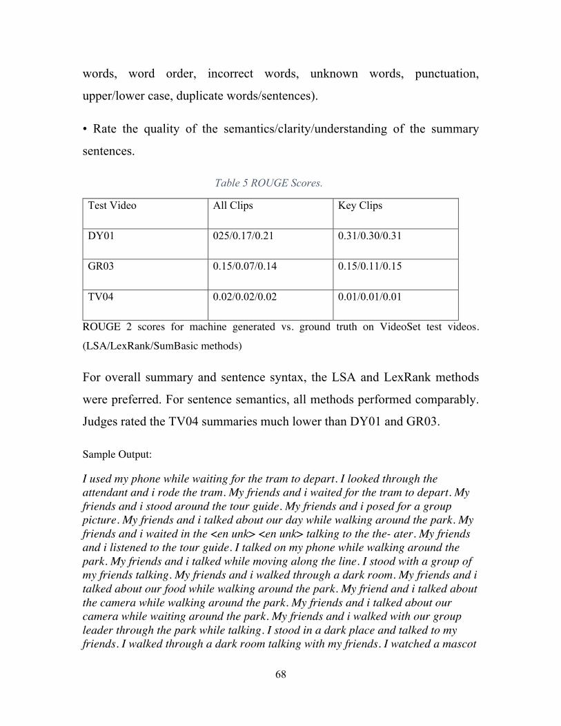
68

words, word order, incorrect words, unknown words, punctuation,

upper/lower case, duplicate words/sentences).

• Rate the quality of the semantics/clarity/understanding of the summary

sentences.

Table 5 ROUGE Scores.

Test Video All Clips Key Clips

DY01 025/0.17/0.21 0.31/0.30/0.31

GR03 0.15/0.07/0.14 0.15/0.11/0.15

TV04 0.02/0.02/0.02 0.01/0.01/0.01

ROUGE 2 scores for machine generated vs. ground truth on VideoSet test videos.

(LSA/LexRank/SumBasic methods)

For overall summary and sentence syntax, the LSA and LexRank methods

were preferred. For sentence semantics, all methods performed comparably.

Judges rated the TV04 summaries much lower than DY01 and GR03.

Sample Output:

I used my phone while waiting for the tram to depart. I looked through the attendant and i rode the tram. My friends and i waited for the tram to depart. My friends and i stood around the tour guide. My friends and i posed for a group picture. My friends and i talked about our day while walking around the park. My friends and i waited in the <en unk> <en unk> talking to the the- ater. My friends and i listened to the tour guide. I talked on my phone while walking around the park. My friends and i talked while moving along the line. I stood with a group of my friends talking. My friends and i walked through a dark room. My friends and i talked about our food while walking around the park. My friend and i talked about the camera while walking around the park. My friends and i talked about our camera while waiting around the park. My friends and i walked with our group leader through the park while talking. I stood in a dark place and talked to my friends. I walked through a dark room talking with my friends. I watched a mascot

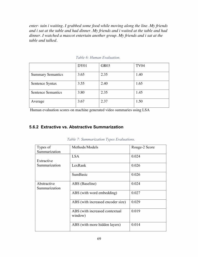
69

enter- tain i waiting. I grabbed some food while moving along the line. My friends and i sat at the table and had dinner. My friends and i waited at the table and had dinner. I watched a mascot entertain another group. My friends and i sat at the table and talked.

Table 6: Human Evaluation.

DY01 GR03 TV04

Summary Semantics 3.65 2.35 1.40

Sentence Syntax 3.55 2.40 1.65

Sentence Semantics 3.80 2.35 1.45

Average 3.67 2.37 1.50

Human evaluation scores on machine generated video summaries using LSA

5.6.2 Extractive vs. Abstractive Summarization

Table 7: Summarization Types Evaluations.

Types of Summarization

Methods/Models Rouge-2 Score

Extractive Summarization

LSA

0.024

LexRank

0.026

SumBasic

0.026

Abstractive Summarization

ABS (Baseline)

0.024

ABS (with word embedding)

0.027

ABS (with increased encoder size)

0.029

ABS (with increased contextual window)

0.019

ABS (with more hidden layers)

0.014

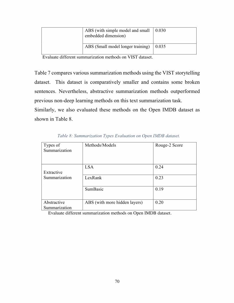
70

ABS (with simple model and small embedded dimension)

0.030

ABS (Small model longer training)

0.035

Evaluate different summarization methods on VIST dataset.

Table 7 compares various summarization methods using the VIST storytelling

dataset. This dataset is comparatively smaller and contains some broken

sentences. Nevertheless, abstractive summarization methods outperformed

previous non-deep learning methods on this text summarization task.

Similarly, we also evaluated these methods on the Open IMDB dataset as

shown in Table 8.

Table 8: Summarization Types Evaluation on Open IMDB dataset.

Evaluate different summarization methods on Open IMDB dataset.

Types of Summarization

Methods/Models Rouge-2 Score

Extractive Summarization

LSA

0.24

LexRank

0.23

SumBasic

0.19

Abstractive Summarization

ABS (with more hidden layers)

0.20

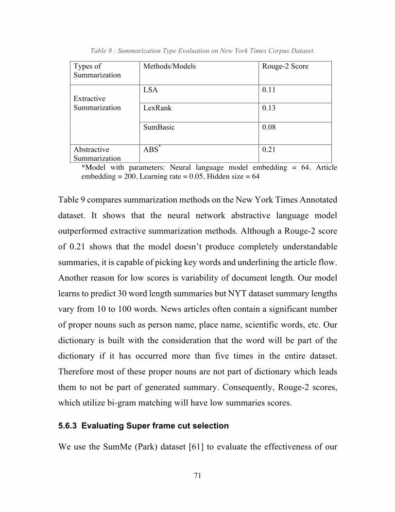
71

Table 9 : Summarization Type Evaluation on New York Times Corpus Dataset.

*Model with parameters: Neural language model embedding = 64, Article embedding = 200, Learning rate = 0.05, Hidden size = 64

Table 9 compares summarization methods on the New York Times Annotated

dataset. It shows that the neural network abstractive language model

outperformed extractive summarization methods. Although a Rouge-2 score

of 0.21 shows that the model doesn’t produce completely understandable

summaries, it is capable of picking key words and underlining the article flow.

Another reason for low scores is variability of document length. Our model

learns to predict 30 word length summaries but NYT dataset summary lengths

vary from 10 to 100 words. News articles often contain a significant number

of proper nouns such as person name, place name, scientific words, etc. Our

dictionary is built with the consideration that the word will be part of the

dictionary if it has occurred more than five times in the entire dataset.

Therefore most of these proper nouns are not part of dictionary which leads

them to not be part of generated summary. Consequently, Rouge-2 scores,

which utilize bi-gram matching will have low summaries scores.

5.6.3 Evaluating Super frame cut selection We use the SumMe (Park) dataset [61] to evaluate the effectiveness of our

Types of Summarization

Methods/Models Rouge-2 Score

Extractive Summarization

LSA

0.11

LexRank

0.13

SumBasic

0.08

Abstractive Summarization

ABS*

0.21

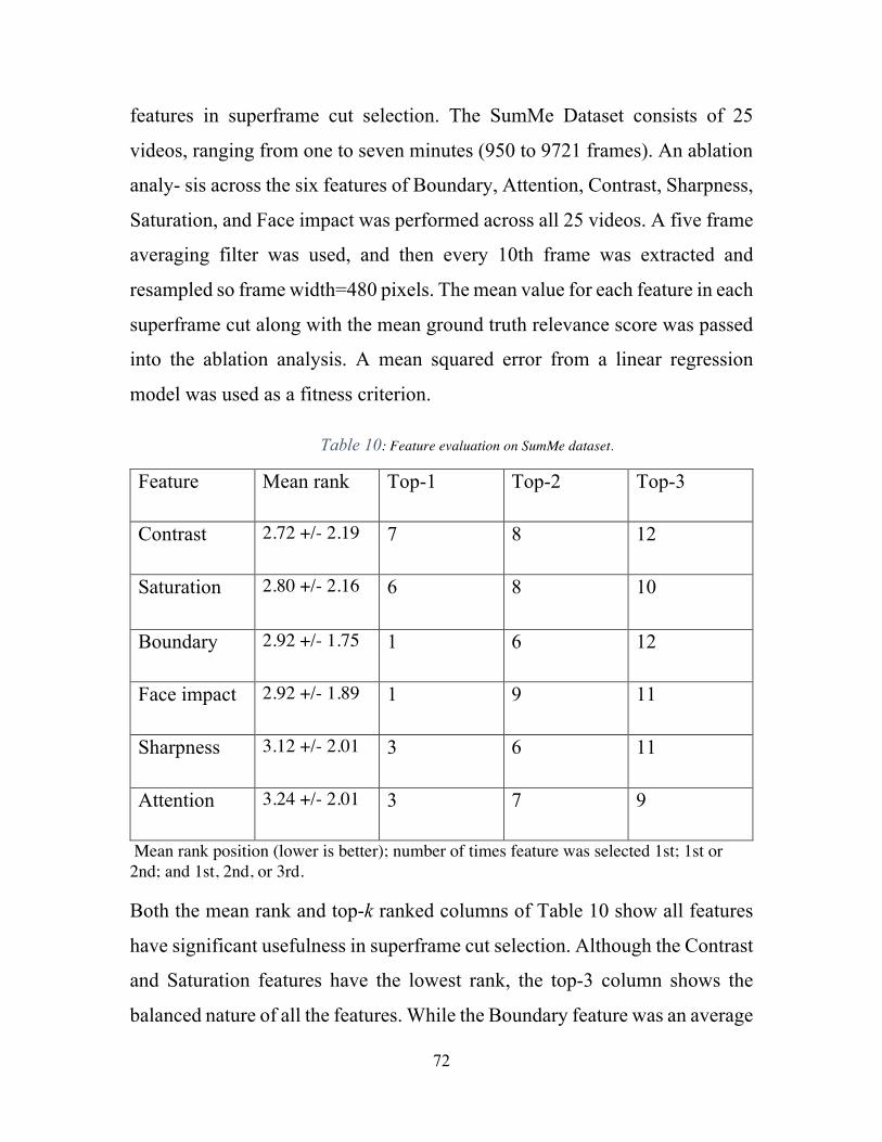
72

features in superframe cut selection. The SumMe Dataset consists of 25

videos, ranging from one to seven minutes (950 to 9721 frames). An ablation

analy- sis across the six features of Boundary, Attention, Contrast, Sharpness,

Saturation, and Face impact was performed across all 25 videos. A five frame

averaging filter was used, and then every 10th frame was extracted and

resampled so frame width=480 pixels. The mean value for each feature in each

superframe cut along with the mean ground truth relevance score was passed

into the ablation analysis. A mean squared error from a linear regression

model was used as a fitness criterion.

Table 10: Feature evaluation on SumMe dataset.

Feature Mean rank Top-1 Top-2 Top-3

Contrast 2.72 +/- 2.19 7 8 12

Saturation 2.80 +/- 2.16 6 8 10

Boundary 2.92 +/- 1.75 1 6 12

Face impact 2.92 +/- 1.89 1 9 11

Sharpness 3.12 +/- 2.01 3 6 11

Attention 3.24 +/- 2.01 3 7 9

Mean rank position (lower is better); number of times feature was selected 1st; 1st or 2nd; and 1st, 2nd, or 3rd.

Both the mean rank and top-k ranked columns of Table 10 show all features

have significant usefulness in superframe cut selection. Although the Contrast

and Saturation features have the lowest rank, the top-3 column shows the

balanced nature of all the features. While the Boundary feature was an average

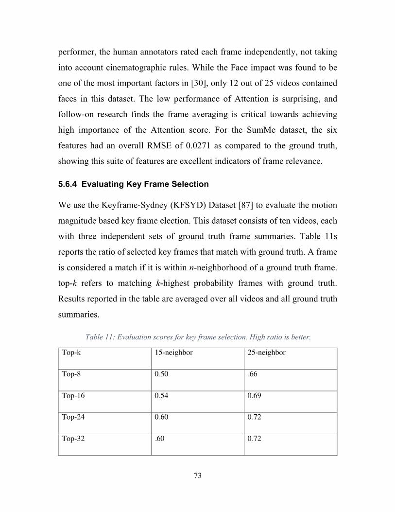
73

performer, the human annotators rated each frame independently, not taking

into account cinematographic rules. While the Face impact was found to be

one of the most important factors in [30], only 12 out of 25 videos contained

faces in this dataset. The low performance of Attention is surprising, and

follow-on research finds the frame averaging is critical towards achieving

high importance of the Attention score. For the SumMe dataset, the six

features had an overall RMSE of 0.0271 as compared to the ground truth,

showing this suite of features are excellent indicators of frame relevance.

5.6.4 Evaluating Key Frame Selection We use the Keyframe-Sydney (KFSYD) Dataset [87] to evaluate the motion

magnitude based key frame election. This dataset consists of ten videos, each

with three independent sets of ground truth frame summaries. Table 11s

reports the ratio of selected key frames that match with ground truth. A frame

is considered a match if it is within n-neighborhood of a ground truth frame.

top-k refers to matching k-highest probability frames with ground truth.

Results reported in the table are averaged over all videos and all ground truth

summaries.

Table 11: Evaluation scores for key frame selection. High ratio is better.

Top-k 15-neighbor 25-neighbor

Top-8 0.50 .66

Top-16 0.54 0.69

Top-24 0.60 0.72

Top-32 .60 0.72

74

Chapter 6 Conclusion

6.1. Key Frame Extraction and Multi-Stream CNNs We propose a novel approach to fuse color spaces and optical flow

information in a single convolutional neural network architecture for state-of-

the-art activity recognition. This study shows that color and motion cues are

necessary and their combination is preferred for accurate action detection. We

studied the performance of key frames over sequentially selected video clips

for large scale human activity classification. We experimentally support that

smartly selected key frames add valuable data to CNNs and hence perform

better than conventional sequential or randomly selected clips. Using key

frames not only provides better results but can significantly reduce the amount

of data being processed. To further reduce computational resources, multi-

stream experiments advocate that lowering down the resolution of

chrominance data stream does not harm performance significantly. Our results

indicate that passing optical flow and YCbCr data into our multi-stream

architecture at key frame locations of videos offer comprehensive feature

learning, which may lead to better understanding of human activity. Such

research can be helpful for video compression, efficient action detection, key-

event detection, motion analysis, etc. with a wide variety of video data.

6.2. Video Summarization This work introduces a novel method for both video summarization and

annotation. Frame to frame motion, frame image quality, as well

cinematographic and consumer preference are uniquely fused together to

determine interesting segments from long videos. Key frames from the most

75

impactful segments are converted to textual annotations using an encoder-

decoder recurrent neural network. Textual annotations are summarized using

extractive methods where LSA, LexRank and SumBasic approaches per-

formed best. Human evaluations of video summaries indicate promising

results. Independent experiments validate both superframe cuts as well as key

frame selection. A key limitation is passing of incorrect superframe or key

frame information to the captioning framework. A potential solution would

be availability of datasets with ground truth on both key segments and

associated captions/summaries. We expect this research to be helpful for

visually challenged people; an efficient video to text system can act as an

instant narrator for them.

6.3. Abstractive Summarization This work explores different types of summarization techniques suitable for

video summarization. Findings suggest that neural network language models

with contextual encoders perform well and generate condensed and sensible

summaries. Neural network based methods give better results on a variety of

datasets and different domains of text sources. One downside is that such

methods require huge amounts of document-summary pairs to train the

network. Longer text will increase context, enabling longer word

dependencies.

Further work in this direction would be to investigate larger datasets, include

word embeddings, and use LSTMs with attention for longer word

dependencies.

76

Bibliography

1. Karpathy, A, Toderici G, Shetty S, Sukthankar T, Li Fei-Fei, . "Large-scale video

classification with convolutional neural networks." Proceedings of the IEEE

conference on Computer Vision and Pattern Recognition 2014: 1725-1732.

2. Johnson, Justin, Andrej Karpathy, and Li Fei-Fei. "DenseCap: Fully Convolutional

Localization Networks for Dense Captioning." arXiv preprint arXiv:1511.07571

(2015).

3. Venugopalan, Subhashini et al. "Translating videos to natural language using deep

recurrent neural networks." arXiv preprint arXiv:1412.4729 (2014).

4. Yao, Li et al. "Describing videos by exploiting temporal structure." Proceedings of

the IEEE International Conference on Computer Vision 2015: 4507-4515.

5. Mnih, Volodymyr, Nicolas Heess, and Alex Graves. "Recurrent models of visual

attention." Advances in Neural Information Processing Systems 2014: 2204-2212.

6. Guadarrama, Sergio et al. "Youtube2text: Recognizing and describing arbitrary

activities using semantic hierarchies and zero-shot recognition." Proceedings of the

IEEE International Conference on Computer Vision 2013: 2712-2719.

7. Krishnamoorthy, Niveda et al. "Generating Natural-Language Video Descriptions

Using Text-Mined Knowledge." AAAI 14 Jun. 2013: 2.

8. Thomason, Jesse et al. "Integrating Language and Vision to Generate Natural

Language Descriptions of Videos in the Wild." COLING Aug. 2014: 9.

9. Karpathy, Andrej, and Li Fei-Fei. "Deep visual-semantic alignments for generating

image descriptions." Proceedings of the IEEE Conference on Computer Vision and

Pattern Recognition 2015: 3128-3137.

10. Rohrbach, Anna et al. "A dataset for movie description." Proceedings of the IEEE

Conference on Computer Vision and Pattern Recognition 2015: 3202-3212.

11. Venugopalan, Subhashini et al. "Sequence to sequence-video to text." Proceedings

of the IEEE International Conference on Computer Vision 2015: 4534-4542.

12. W. Wolf, “Key frame selection by motion analysis,” in Acoustics, Speech, and

Signal Processing, 1996. ICASSP-96. Conference Proceedings., 1996 IEEE

International Conference on, vol. 2. IEEE, 1996, pp. 1228– 1231

77

13. Sankaran, Baskaran, et al. "Temporal attention model for neural machine

translation." arXiv preprint arXiv:1608.02927 (2016).

14. Soomro, Khurram, Amir Roshan Zamir, and Mubarak Shah. "UCF101: A dataset

of 101 human actions classes from videos in the wild." arXiv preprint

arXiv:1212.0402 (2012).

15. X. Hou, J. Harel, and C. Koch. Image signature: Highlighting sparse salient regions.

Pattern Analysis and Machine Intelligence, IEEE Transactions on, 34(1):194–201,

2012

16. N. Ejaz, I. Mehmood, and S. W. Baik. Efficient visual attention based framework

for extracting key frames from videos. Signal Processing: Image Communication,

28(1):34–44, 2013.

17. D. G. Lowe, “Object recognition from local scale-invariant features,” in Computer

vision, 1999. The proceedings of the seventh IEEE international conference on, vol.

2. Ieee, 1999, pp. 1150–1157.

18. N. Dalal and B. Triggs, “Histograms of oriented gradients for human detection,” in

Computer Vision and Pattern Recognition, 2005. CVPR 2005. IEEE Computer

Society Conference on, vol. 1. IEEE, 2005, pp. 886–893.

19. A. Krizhevsky, I. Sutskever, and G. E. Hinton, “Imagenet classification with deep

convolutional neural networks,” in Advances in neural information processing

systems, 2012, pp. 1097–1105.

20. C. Szegedy, W. Liu, Y. Jia, P. Sermanet, S. Reed, D. Anguelov, D. Erhan, V.

Vanhoucke, and A. Rabinovich, “Going deeper with convolutions,” in Proceedings

of the IEEE Conference on Computer Vision and Pattern Recognition, 2015, pp. 1–

9.

21. A. Nguyen, J. Yosinski, and J. Clune, “Deep neural networks are easily fooled:

High confidence predictions for unrecognizable images,” in Computer Vision and

Pattern Recognition (CVPR), 2015 IEEE Conference on. IEEE, 2015, pp. 427–436.

22. S. Chaabouni, J. Benois-Pineau, O. Hadar, and C. B. Amar, “Deep learning for

saliency prediction in natural video,” 2016.

78

23. K. Simonyan and A. Zisserman, “Two-stream convolutional networks for action

recognition in videos,” in Advances in Neural Information Processing Systems,

2014, pp. 568–576.

24. A. Karpathy, G. Toderici, S. Shetty, T. Leung, R. Sukthankar, and L. Fei-Fei,

“Large-scale video classification with convolutional neural networks,” in

Proceedings of the IEEE conference on Computer Vision and Pattern Recognition,

2014, pp. 1725–1732.

25. K. Fukushima, “Neocognitron: A self-organizing neural network model for a

mechanism of pattern recognition unaffected by shift in position,” Biological

cybernetics, vol. 36, no. 4, pp. 193–202, 1980.

26. M. Riesenhuber and T. Poggio, “Hierarchical models of object recognition in

cortex,” Nature neuroscience, vol. 2, no. 11, pp. 1019–1025, 1999.

27. J. Liu, J. Luo, and M. Shah, “Recognizing realistic actions from videos in the wild,”

in Computer Vision and Pattern Recognition, 2009. CVPR 2009. IEEE Conference

on. IEEE, 2009, pp. 1996–2003.

28. R. Chaudhry, A. Ravichandran, G. Hager, and R. Vidal, “Histograms of oriented

optical flow and binet-cauchy kernels on nonlinear dynamical systems for the

recognition of human actions,” in Computer Vision and Pattern Recognition, 2009.

CVPR 2009. IEEE Conference on. IEEE, 2009, pp. 1932–1939.

29. I. Laptev, M. Marszalek, C. Schmid, and B. Rozenfeld, “Learning realistic human

actions from movies,” in Computer Vision and Pattern Recognition, 2008. CVPR

2008. IEEE Conference on, June 2008, pp. 1–8.

30. H. Wang and C. Schmid, “Action recognition with improved trajectories,” in 2013

IEEE International Conference on Computer Vision, Dec 2013, pp. 3551–3558.

31. H. Wang, A. Klser, C. Schmid, and C. L. Liu, “Action recognition by dense

trajectories,” in Computer Vision and Pattern Recognition (CVPR), 2011 IEEE

Conference on, June 2011, pp. 3169–3176.

32. R. Girshick, J. Donahue, T. Darrell, and J. Malik, “Rich feature hierarchies for

accurate object detection and semantic segmentation,” in Proceedings of the IEEE

conference on computer vision and pattern recognition, 2014, pp. 580–587.

79

33. P. Sermanet, D. Eigen, X. Zhang, M. Mathieu, R. Fergus, and Y. LeCun, “Overfeat:

Integrated recognition, localization and detection using convolutional networks,”

arXiv preprint arXiv:1312.6229, 2013.

34. C. Farabet, C. Couprie, L. Najman, and Y. LeCun, “Learning hierarchical features

for scene labeling,” Pattern Analysis and Machine Intelligence, IEEE Transactions

on, vol. 35, no. 8, pp. 1915–1929, 2013.

35. H. Jhuang, T. Serre, L. Wolf, and T. Poggio, “A biologically inspired system for

action recognition,” in Computer Vision, 2007. ICCV 2007. IEEE 11th

International Conference on. Ieee, 2007, pp. 1–8.

36. S. Ji, W. Xu, M. Yang, and K. Yu, “3d convolutional neural networks for human

action recognition,” Pattern Analysis and Machine Intelligence, IEEE Transactions

on, vol. 35, no. 1, pp. 221–231, 2013.

37. G. W. Taylor, R. Fergus, Y. LeCun, and C. Bregler, “Convolutional learning of

spatio-temporal features,” in Computer Vision–ECCV 2010. Springer, 2010, pp.

140–153.

38. Q. V. Le, W. Y. Zou, S. Y. Yeung, and A. Y. Ng, “Learning hierarchical invariant

spatio-temporal features for action recognition with independent subspace

analysis,” in Computer Vision and Pattern Recognition (CVPR), 2011 IEEE

Conference on. IEEE, 2011, pp. 3361–3368.

39. C.-B. Ng, Y.-H. Tay, and B.-M. Goi, “Comparing image representations for

training a convolutional neural network to classify gender,” in Artificial

Intelligence, Modelling and Simulation (AIMS), 2013 1st International Conference

on. IEEE, 2013, pp. 29–33.

40. G. Farneback, “Two-frame motion estimation based on polynomial ¨ expansion,”

in Image analysis. Springer, 2003, pp. 363–370.

41. G. Gkioxari and J. Malik, “Finding action tubes,” in Proceedings of the IEEE

Conference on Computer Vision and Pattern Recognition, 2015, pp. 759–768.

42. K. Soomro, A. R. Zamir, and M. Shah, “Ucf101: A dataset of 101 human actions

classes from videos in the wild,” arXiv preprint arXiv:1212.0402, 2012.

80

43. A. Girgensohn and J. Boreczky, “Time-constrained keyframe selection technique,”

in Multimedia Computing and Systems, 1999. IEEE International Conference on,

vol. 1. IEEE, 1999, pp. 756–761.

44. S. Ioffe and C. Szegedy, “Batch normalization: Accelerating deep network training

by reducing internal covariate shift,” CoRR, vol. abs/1502.03167, 2015. [Online].

Available: http://arxiv.org/abs/1502.03167

45. N. Srivastava, G. Hinton, A. Krizhevsky, I. Sutskever, and R. Salakhutdinov,

“Dropout: A simple way to prevent neural networks from over- fitting,” The Journal

of Machine Learning Research, vol. 15, no. 1, pp. 1929–1958, 2014.

46. M. Gygli, H. Grabner, and L. Van Gool. Video summarization by learning

submodular mixtures of objectives. In Proceedings of the IEEE Conference on

Computer Vision and Pattern Recognition, pages 3090–3098, 2015.

47. K. Zhang, W.-L. Chao, F. Sha, and K. Grauman. Summary transfer: Exemplar-

based subset selection for video summarization. arXiv preprint arXiv:1603.03369,

2016.

48. S. Kulhare, S. Sah, S. Pillai and R. Ptucha. Key frame extraction for salient activity

recognition. International Conference for Pattern Recognition, 2017.

49. H. Wang, M. M. Ullah, A. Klaser, I. Laptev, C. Schmid, et al. Evaluation of local

spatio-temporal features for action recognition. In BMVC, 2009

50. J. C. Niebles, C.-W. Chen, and L. Fei-Fei. Modeling temporal structure of

decomposable motion segments for activity classification. In ECCV, pages 392–

405. Springer, 2010.

51. J. Sivic and A. Zisserman. Video Google: A text retrieval approach to object

matching in videos. In ICCV, 2003. 2

52. Mikolajczyk, Krystian, and Cordelia Schmid. "Indexing based on scale invariant

interest points." Computer Vision, 2001. ICCV 2001. Proceedings. Eighth IEEE

International Conference on. Vol. 1. IEEE, 2001.

53. Scovanner, Paul, Saad Ali, and Mubarak Shah. "A 3-dimensional sift descriptor and

its application to action recognition." Proceedings of the 15th ACM international

conference on Multimedia. ACM, 2007.

81

54. A. Klaser, M. Marszałek, and C. Schmid. A spatio-temporal descriptor based on

3D-gradients. In BMVC, 2008.

55. G. Willems, T. Tuytelaars, and L. Gool. An efficient dense and scale invariant

spatio-temporal interest point detector. In ECCV, 2008.

56. I. Laptev. On space-time interest points. IJCV, 64(2-3):107–123, 2005.

57. Baccouche, M., Mamalet, F., Wolf, C., Garcia, C., & Baskurt, A. (2011,

November). Sequential deep learning for human action recognition.

In International Workshop on Human Behavior Understanding (pp. 29-39).

Springer, Berlin, Heidelberg.

58. Harris, Chris, and Mike Stephens. "A combined corner and edge detector." Alvey

vision conference. Vol. 15. No. 50. 1988.

59. Tran, D., Bourdev, L., Fergus, R., Torresani, L., & Paluri, M. (2015). Learning

spatiotemporal features with 3d convolutional networks. In Proceedings of the

IEEE international conference on computer vision (pp. 4489-4497).

60. Z.Lu and K.Grauman. Story-driven summarization for egocentric video. In

Proceedings of the IEEE CVPR, pages 2714–2721, 2013.

61. M.Gygli, H.Grabner, H.Riemenschneider, and L.Van Gool. Creating summaries

from user videos. In European conference on computer vision, pages 505–520.

Springer, 2014.

62. Y. Song, J. Vallmitjana, A. Stent, and A. Jaimes. Tvsum: Summarizing web videos

using titles. In Proceedings of the IEEE Conference on Computer Vision and

Pattern Recogni- tion, pages 5179–5187, 2015.

63. B. Gong, W.-L. Chao, K. Grauman, and F. Sha. Diverse sequential subset selection

for supervised video summarization. In Advances in Neural Information Processing

Systems, pages 2069–2077, 2014.

64. K. Zhang, W.-L. Chao, F. Sha, and K. Grauman. Video summarization with long

short-term memory. arXiv preprint arXiv:1605.08110, 2016. O. Vinyals, A.

Toshev, S. Bengio, and D. Erhan. Show and tell: A neural image caption generator.

In Proceedings of the IEEE Conference on Computer Vision and Pattern Recogni-

tion, pages 3156–3164, 2015.

82

65. Y.Ke, X.Tang, and F.Jing. The design of high-level features for photo quality

assessment. In Computer Vision and Pat- tern Recognition, 2006 IEEE Computer

Society Conference on, volume 1, pages 419–426. IEEE, 2006.

66. R. Datta, D. Joshi, J. Li, and J. Z. Wang. Studying aesthetics in photographic images

using a computational approach. In ECCV 2006, pages 288–301. Springer, 2006.

67. J. Ghosh, Y. J. Lee, and K. Grauman. Discovering important people and objects for

egocentric video summarization. In 2012 IEEE Conference on Computer Vision

and Pattern Recognition, pages 1346–1353. IEEE, 2012.

68. R. Ptucha, D. Kloosterman, B. Mittelstaedt, and A. Loui. Automatic image

assessment from facial attributes. In IS&T/SPIE Electronic Imaging, pages

90200C–90200C. In- ternational Society for Optics and Photonics, 2014.

69. J. Donahue, L. Anne Hendricks, S. Guadarrama, M. Rohrbach, S. Venugopalan, K.

Saenko, and T. Dar- rell. Long-term recurrent convolutional networks for visual

recognition and description. In Proceedings of the IEEE CVPR, pages 2625–2634,

2015.

70. X. Chen and C. L. Zitnick. Learning a recurrent visual representation for image

caption generation. 2015.

71. H. Yu, J. Wang, Z. Huang, Y. Yang, and W. Xu. Video paragraph captioning using

hierarchical recurrent neural networks. arXiv preprint arXiv:1510.07712, 2015.

72. H. P. Luhn. The automatic creation of literature abstracts. IBM Journal of research

and development, 2(2):159–165, 1958.

73. H. P. Edmundson. New methods in automatic extracting. Journal of the ACM

(JACM), 16(2):264–285, 1969.

74. A. Nenkova and L. Vanderwende. The impact of frequency on summarization.

Microsoft Research, Redmond, Washing- ton, Tech. Rep. MSR-TR-2005-101,

2005.

75. L. Vanderwende, H. Suzuki, C. Brockett, and A. Nenkova. Beyond sumbasic: Task-

focused summarization with sen- tence simplification and lexical expansion.

Information Pro- cessing & Management, 43(6):1606–1618, 2007.

83

76. G. Erkan and D. R. Radev. Lexrank: Graph-based lexical centrality as salience in

text summarization. Journal of Arti- ficial Intelligence Research, pages 457–479,

2004.

77. R. Mihalcea and P. Tarau. Textrank: Bringing order into texts. 2004.

78. A. Haghighi and L. Vanderwende. Exploring content mod- els for multi-document

summarization. In Proceedings of Human Language Technologies: The 2009

Annual Confer- ence of the North American Chapter of the Association for

Computational Linguistics, pages 362–370. Association for Computational

Linguistics, 2009.

79. A. Nenkova, S. Maskey, and Y. Liu. Automatic summarization. In Proceedings of

the 49th Annual Meeting of the Asso- ciation for Computational Linguistics:

Tutorial Abstracts of ACL 2011, page 3. Association for Computational Linguis-

tics, 2011.

80. T. Hirao, Y. Yoshida, M. Nishino, N. Yasuda, and M. Nagata. Single-document

summarization as a tree knapsack problem. In EMNLP, volume 13, pages 1515–

1520, 2013.

81. G. Durrett, T. Berg-Kirkpatrick, and D. Klein. Learning- based single-document

summarization with compression and anaphoricity constraints. arXiv preprint

arXiv:1603.08887, 2016.

82. K. He, X. Zhang, S. Ren, and J. Sun. Deep residual learning for image recognition.

arXiv preprint arXiv:1512.03385, 2015.

83. S. Hochreiter and J. Schmidhuber. Long short-term memory. Neural computation,

9(8):1735–1780, 1997.

84. C.-Y. Lin. Rouge: A package for automatic evaluation of summaries. In Text

summarization branches out: Proceed- ings of the ACL-04 Workshop, volume 8.

Spain, 2004.

85. S. Yeung, A. Fathi, and L. Fei-Fei. Videoset: Video evalua- tion through text. arXiv

preprint arXiv:1406.5824, 2014.

86. D. L. Chen and W. B. Dolan. Collecting highly parallel data for paraphrase

evaluation. In Proceedings of the 49th Annual Meeting of the Association for

84

Computational Linguistics: Human Language Technologies-Volume 1, pages 190–

200. Association for Computational Linguistics, 2011.

87. G. Guan, Z. Wang, S. Lu, J. D. Deng, and D. D. Feng. Keypoint-based keyframe

selection. IEEE Tran on Circuits and Systems for Video Technology, 23(4):729–

734, 2013.

88. Hahn, Udo, and Martin Romacker. "Text Understanding for Knowledge Base

Generation in the SYNDICATE System." Database and Expert Systems

Applications. Springer Berlin/Heidelberg, 1999.

89. Rush, Alexander M., Sumit Chopra, and Jason Weston. "A neural attention model

for abstractive sentence summarization." arXiv preprint arXiv:1509.00685 (2015).

90. Bengio, Yoshua, "A neural probabilistic language model." Journal of machine

learning research 3.Feb (2003): 1137-1155.

91. Ferraro, Francis, Nasrin Mostafazadeh, Ishan Misra, Aishwarya Agrawal, Jacob

Devlin, Ross Girshick, Xiaodong He, "Visual storytelling." arXiv preprint

arXiv:1604.03968 (2016).

92. Thomason, J., Venugopalan, S., Guadarrama, S., Saenko, K., & Mooney, R. J.

(2014, August). Integrating Language and Vision to Generate Natural Language

Descriptions of Videos in the Wild. In Coling (Vol. 2, No. 5, p. 9).

93. Thomason, J., Venugopalan, S., Guadarrama, S., Saenko, K., & Mooney, R. J.

(2014, August). Integrating Language and Vision to Generate Natural Language

Descriptions of Videos in the Wild. In Coling (Vol. 2, No. 5, p. 9).

94. Wu, Z., Jiang, Y. G., Wang, X., Ye, H., & Xue, X. (2016, October). Multi-stream

multi-class fusion of deep networks for video classification. In Proceedings of the

2016 ACM on Multimedia Conference (pp. 791-800). ACM.

95. Bengio, Yoshua, Patrice Simard, and Paolo Frasconi. "Learning long-term

dependencies with gradient descent is difficult." IEEE transactions on neural

networks 5.2 (1994): 157-166.

96. Hochreiter, Sepp, and Jürgen Schmidhuber. "Long short-term memory." Neural

computation 9.8 (1997): 1735-1780.

85

97. Cho, K., Van Merriënboer, B., Gulcehre, C., Bahdanau, D., Bougares, F., Schwenk,

H., & Bengio, Y. (2014). Learning phrase representations using RNN encoder-

decoder for statistical machine translation. arXiv preprint arXiv:1406.1078.

98. Wu, Z., Wang, X., Jiang, Y. G., Ye, H., & Xue, X. (2015, October). Modeling

spatial-temporal clues in a hybrid deep learning framework for video classification.

In Proceedings of the 23rd ACM international conference on Multimedia (pp. 461-

470). ACM.