Deep infrared studies of massive high redshift galaxies

Deep infrared studies of massive high redshift galaxiesLabbé, I.

CitationLabbé, I. (2004, October 13). Deep infrared studies of massive high redshift galaxies.Retrieved from https://hdl.handle.net/1887/578 Version: Publisher's Version

License: Licence agreement concerning inclusion of doctoral thesis in theInstitutional Repository of the University of Leiden

Downloaded from: https://hdl.handle.net/1887/578 Note: To cite this publication please use the final published version (if applicable).

https://hdl.handle.net/1887/license:5

https://hdl.handle.net/1887/license:5

https://hdl.handle.net/1887/578

CHAPTER

FIVE

T h e C o lo r M a g n itu d e D istrib u tio n o fFie ld G a la x ie s a t 1 < z < 3

the ev o lu tio n a n d m o d elin g o f the b lu e seq u en ce

ABSTRAC T

We u se d eep near-infrared V L T / IS AAC imag ing to stu d y the rest-frameco lo r-mag nitu d e d istribu tio n o f infrared selected g alax ies in the red shiftrang e 1 < z < 3. We fi nd a well-d efi ned blu e peak o f star-fo rming g alax ies atall red shifts. T he blu e g alax ies po pu late a c o lo r-mag nitu d e relatio n (CM R ),su ch that mo re lu mino u s g alax ies in the rest-frame V -band tend to havered d er u ltravio let-to -o ptical c o lo rs. T he slo pe o f the CM R d o es no t evo lvewith time, and is similar to the slo pe o f blu e, late-type g alax ies in the lo calu niverse. Analysis o f spectra o f nearby late-type g alax ies su g g ests that thesteepness o f the slo pe can be fu lly ex plained by the o bserved c o rrelatio n o fd u st c o ntent with o ptical lu mino sity. T he zero po int o f the blu e CM R at ag iven mag nitu d e red d ens smo o thly from z = 3 to z = 0 , lik ely refl ecting anincrease o f the mean stellar ag e and an increase in the mean d u st o pac ity o fblu e-seq u ence g alax ies. A d istinct featu re is that the c o lo r scatter aro u nd thez ∼ 3 CM R is asymmetric , with a blu e “ rid g e” and a sk ew toward s red c o l-o rs. We have ex plo red which types o f star fo rmatio n histo ries can repro d u cethe scatter and the sk ewed shape o f the c o lo r d istribu tio n. T hese inc lu d edmo d els with co nstant star fo rmatio n rates and su d d en c u to ff s, ex po nentiallyd ec lining star fo rmatio n rates, bu rst mo d els, and mo d els with episo d ic starfo rmatio n. T he episo d ic mo d els repro d u ced the c o lo r d istribu tio n best, withq u iescent perio d s lasting 30 -5 0 % o f the leng th o f an active perio d , and d u ra-tio n o f the d u ty cyc le between 15 0 M yr to 1 G yr. T he episo d ic star fo rmatio nin these mo d els reju venate the g alax ies d u ring each episo d e, mak ing it sig -nifi cantly blu er than a g alax y with co nstant star fo rmatio n o f the same ag e.T his c o u ld be a so lu tio n o f the enigmatic o bservatio n that z = 3 g alax ies aremu ch blu er than ex pected if they were as o ld as the u niverse. F inally, thec o lo r d istribu tio n has a stro ng tail o f very red g alax ies. T he relative nu mbero f red g alax ies inc reases sharply from z ∼ 3 to z ∼ 1. T he rest-frame V -band lu mino sity d ensity in lu mino u s blu e-seq u ence g alax ies is c o nstant, o rd ec reases, whereas that in red g alax ies rises with time. We are viewing thepro g ressive fo rmatio n o f red , passively evo lving g alax ies.

Ivo L a b b e , M a rijn Fra n x , G re g ory R u d n ick , N a ta sch a M . Forste r S ch re ib e r,

E m a n u e le D a d d i, Pie te r G . va n D ok k u m , K on ra d K u ijk e n , A la n M oorw ood ,

H a n s-Wa lte r R ix , H u u b R ottg e rin g , Ig n a c io Tru jillo, A rje n va n d e r Wel, Pa u l va n

d e r Werf, & L ottie va n S ta rk e n b u rg

1045 T h e co lo r m a gn itu d e d istribu tio n o f fi eld ga la xies a t 1 < z < 3: th e evo lu tio n

a n d m od elin g o f th e blu e sequ en ce

1 Introduction

The formation and evolu tion of g alax ies is a complex process, involving theg rowth of dark-matter stru ctu re from the g radu al hierarchical merg ing of

smaller fragments (e.g ., W hite & Frenk 19 9 1; K au ff mann & W hite 19 9 3), theaccretion of g as, the formation of stars, and feedback from su pernovae and blackholes. Presently, the theories describing the g rowth of larg e-scale dark-matterstru ctu re are thou g ht to be well-constrained (Freedman et al. 2001; Efstathiou etal. 2002; S perg el et al. 2003), bu t the formation history of the stars inside thedark-matter halos is still poorly u nderstood. N either hydrodynamical simu lations(e.g ., K atz & G u nn 19 9 1; S pring el et.al. 2001; S teinmetz & N avarro 2002) norstate-of-the-art semianalytic models (e.g ., K au ff mann, W hite, & G u iderdoni 19 9 3;S omerville & Primack 19 9 9 ; Cole, L acey, B au g h, & Frenk 2000) provide u niq u epredictions for the formation of the stars in g alax ies, g iven the larg e parameterspace available to these models. D irect observations are critical to constrain them.

S pecifi cally the observations of massive g alax ies provide strong tests for pictu resof g alax y formation, as their bu ild-u p can be directly observed from hig h redshiftto the present epoch. The larg est samples of hig h-redshift g alax ies to date havebeen selected by their rest-frame U V lig ht, throu g h the L yman B reak techniq u e(L B G s; S teidel et al. 19 9 6 a,b, 2003). U nfortu nately, the rest-frame U V lig ht ishig hly su sceptible to du st and not a g ood measu re of the nu mber of intermediateand low mass stars, which may dominate the stellar mass. In fact, rest-frameoptical observations have shown L B G s to be relatively low mass (M ∼ 1010M¯),u nobscu red, star-forming g alax ies (e.g ., Papovich, D ickinson, & Ferg u son 2001;S hapley et al. 2001).

The rest-frame optical lig ht is already mu ch less sensitive to the eff ects of du stobscu ration and on-g oing star formation than the U V , and it is ex pected to be abetter tracer of stellar mass. Recent advances in near-infrared (N IR) capabilitieson larg e telescopes are now making it possible to select statistically meaning fu lsamples of g alax ies by their rest-frame optical lig ht ou t to z ∼ 3. In this contex twe started the Faint Infrared Ex trag alactic S u rvey (FIRES ; Franx et al. 2000), adeep optical-to-infrared mu lticolor su rvey of N IR-selected g alax ies. The rest-frameoptical observations are also u sefu l as mu ch of ou r knowledg e in the local u niverseis based on stu dies at these waveleng ths.

A particu lar diag nostic of g alax y formation is the shape of the g alax y lu mi-nosity and mass fu nctions as a fu nction of the spectral type. In the local u niversethese distribu tions have been determined in g reat detail (e.g ., S trateva et al. 2001;N orberg et al. 2002; B lanton et al. 2003; K au ff mann et al 2003). W hile a pre-cise characterisation of the local distribu tions can strong ly constrain the models,powerfu l tests can also be made u sing their evolu tion as a fu nction of redshift.For ex ample, B ell et al. (2004a,2004b) show that the V -band lu minosity den-sity of photometrically selected early-type g alax ies is nearly constant in the rang e0.2 < z < 1.1, su g g esting an increase in stellar mass of passively evolving g alax ies

5.1 Introduction 105

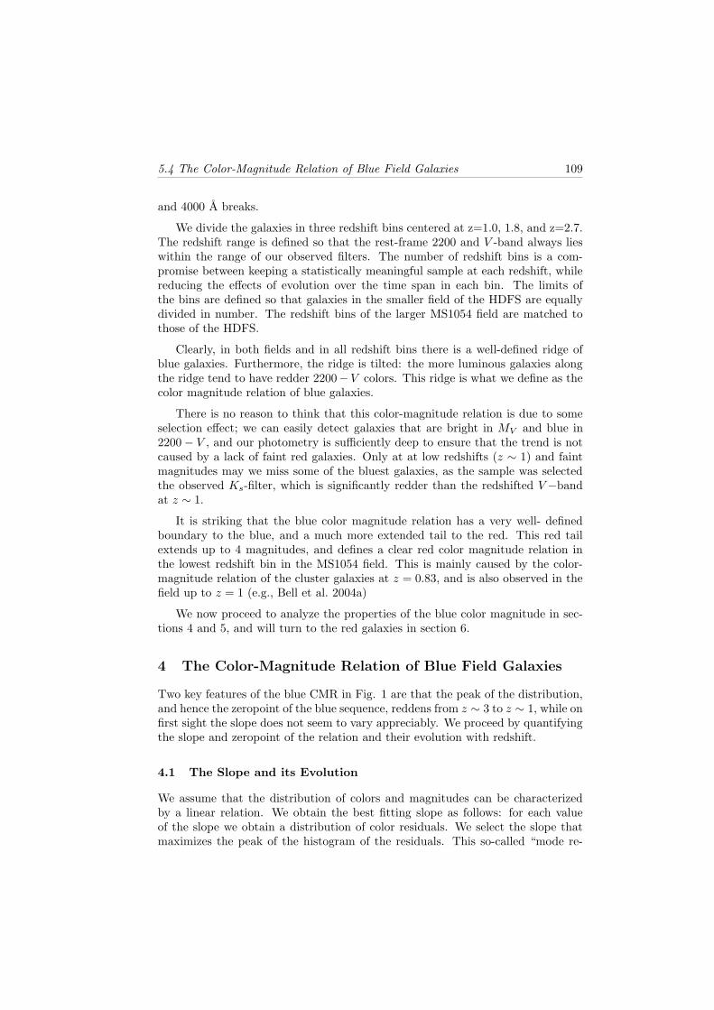
over this range. This is not expected from the simplest collapse models, where allgalaxies form at high redshift and evolve passively to the present-day.

Different constraints on galaxy formation come from correlations between inte-grated galaxy properties. For example, morphologically early-type galaxies in thelocal universe and distant clusters populate a well-defined color-magnitude rela-tion (CMR), which is thought to refl ect a sequence of increasing metallicity withstellar mass (e.g., Bower, Lucey, & Ellis 1992; Schweizer & Seitzer 1992; Kodama& Arimoto 1997 ). The small scatter of this relation implies that early type galaxiesformed most of their stars at high redshift (e.g., van Dokkum et al. 1998 ). Blue,star forming, late-type galaxies also display a color-magnitude relation (Chester &Roberts 1964; Visvanathan 198 1; Tully, Mould, & Aaronson 198 2), but the scatteris larger (Griersmith 198 0), and its origin is probably more complex; it has beeninterpreted as a sequence in the mean stellar age (Peletier & de Grijs 1998 ), dustattenuation (Tully et al. 1998 ), and/ or metallicity (Z aritsky, Kennicutt, & Huchra1994, Bell & De J ong 2000).

Interestingly, Papovich, Dickinson, & Ferguson (2001) found a color-magnituderelation for blue, star-forming galaxies at z ∼ 3, from a sample of NIR-selectedgalaxies in the Hubble Deep Field North (HDFN). The trend, which is also seen inthe similar field of the Hubble Deep Field South (Labbe et al. 2003), is such thatgalaxies more luminous in the rest-frame V −band, tend to have redder ultraviolet-to-optical colors. A distinct aspect of the high-redshift CMR, is that the galaxiesare asymmetrically distributed around the relation, with a well-defined blue enve-lope (Papovich et al. 2004).

Studies of colors and magnitudes of star-forming galaxies at z > 2 also raisedquestions. A particular puzzle was presented by modeling of their stellar popu-lations, which implied average luminosity weighted ages of a few 100 Myr, muchyounger than the age of the universe at these redshifts (e.g., Papovich, Dickinson,& Ferguson 2001; Shapley et al. 2001). From this, and from the relative absence ofcandidates for red, non star-forming galaxies in the HDFN it was suggested thatstar formation in LBGs occurs with short duty cycles and a timescale between starformation events of . 1 Gyr.

In this paper, we investigate the evolution of the rest-frame colors of galaxiesas a function of redshift in the range 1 . z . 3. The deep optical-to-NIR imagingand the homogeneous photometry of the FIRES project is excellently suited forsuch studies, and we use it to analyze rest-frame ultraviolet-to-optical colors andmagnitudes of a sample of 147 5 Ks-band selected galaxies.

We focus on the galaxies that populate the blue peak of galaxies at low andhigh redshift. We wish to understand the nature of the blue color-magnituderelation, the evolution of the colors towards high redshift, and the origin of theconspicious skewed color distribution around the CMR at z ∼ 3. For the latter weexplore models with different types of star formation histories that might producesuch distributions. Finally, we chart the evolution of the relative number of red

1065 The color magnitude distribution of field galaxies at 1 < z < 3: the evolution

and modeling of the blue sequence

galaxies over the redshift range 1 . z . 3.

This paper is organized as follows. We present the data in §2, describe the colormagnitude distribution of FIRES galaxies in §3, analyze the blue color-magnituderelation in §4, and model the scatter of galaxies around the blue CMR in §5.Finally, §6 presents the evolution of the red galaxy fraction. Where necessary, weadopt an ΩM = 0.3,ΩΛ = 0.7, and H0 = 70 km s−1Mpc−1 cosmology. We usemagnitudes calibrated to models for Vega throughout.

2 T he D ata

2.1 T h e O b se rv a tio n s a n d S a m p le S e le c tio n

The observations were obtained as part of the public Faint Infrared ExtragalacticSurvey (FIRES; Franx et al. 2000) the deepest groundbased NIR survey to date.We cover two fields with existing deep optical WFPC2 imaging from the H ubble

S pace Telescope (HST): the WPFC2-field of HDFS, and the field around the z =0.83 cluster MS1054-03. The observations, data reduction, and assembly of thecatalog source catalogs are presented in detail by Labbe et al. (2003) for the HDFSand Forster Schreiber et al. (2004a) for the MS1054 field.

Briefly, we observed in the NIR Js,H, and Ks bands with the Infrared Spec-trometer and Array Camera (ISAAC; Moorwood 1997) at the Very Large Telescope

(VLT). In the HDFS, a total of 101.5 hours was invested in a single 2.5′ × 2.5′

pointing, resulting in the deepest groundbased NIR imaging, and the deepestK−band to date, even from space. We complemented the existing deep opticalHST WFPC2 imaging in the U3 00, B4 5 0, V6 06 , I8 14 bands (Casertano et al. 2000).A further 77 hours of NIR imaging was spent on a mosaic of four ISAAC point-ings centered on the z = 0.83 foreground cluster MS1054-03, reaching somewhatshallower depths. We complemented the data with WFPC2 mosaics in the V6 06

and I8 14 bands (van Dokkum et al. 2000), and collected additional imaging withthe VLT FO RS1 instrument in the U,B, and V bands (Forster Schreiber et al.2004a). In both surveyed fields the effective seeing in the final NIR images was≈ 0.′′45 − 0.′′55 FWHM.

We detect objects in the Ks-band using version 2.2.2 of the SExtractor software((Bertin & Arnouts 1996). For consistent photometry accross all bands, all imageswere aligned, and accurately PSF-matched to the filter in which the image qualitywas worst. Stellar curve of growth analysis indicates that the fraction of enclosedflux agrees to better than 3% for the apertures relevant to our color measurements.The color measurements were done in a customized isophotal aperture definedfrom the Ks−image. The estimate of total flux in the Ks-band was computedusing SExtractors A UTO aperture for isolated sources, and in an adaptive circularaperture for blended sources. In both cases, a minimal aperture correction for thelight lost by a point source was applied. Photometric uncertainties were derivedempirically from the flux distribution in apertures placed on empty parts of the

5.2 The D ata 107

maps. For details concerning all aspects of the photometric measurements, seeLabbe et al. 2003. The total 5−σ limiting depth for point sources are K tots

s = 23.8for the HDFS, and 23.1 for the MS1054-field.

2.2 P hotometric R edshifts and R est-F rame C olors

Photometric redshifts were estimated by fitting a linear combination of redshiftedempirical galaxy spectra, and a 10 Myr old simple stellar population model (1999version of Bruzual A. & Charlot 1993) to the observed flux points. The algorithmis described in detail by Rudnick et al. (2001, 2003). We adopt a minimux fluxerror of 5% for all bands to account for zeropoint uncertainties and for mismatchesbetween the observations and the photo-z template set.

Monte-Carlo simulations were used to estimate the errors δzp h ,MC on the pho-tometric redshifts. These errors reflect the photometric uncertainties, templatemismatch, and the possibility of secondary solutions. We determined the accu-ray of the technique from comparisons to the available spectroscopy in each field.We find δz =< |zsp e c − zp h ot|/(1 + zsp e c ) >= 0.07, and δz = 0.05 for sources atz ≥ 2. The errors calculated from simulations δzp h ,MC are consistent with this.We identified and removed stars using the method described in Rudnick et al.(2003).

We combine the observed SEDs and photometric redshifts to derive rest-frameluminosties Lre st

λ . We used a method of estimating Lre stλ that interpolates di-

rectly between the observed fluxes, using the templates as a guide. The rest-framephometric system, and details on estimating Lre st

λ are described extensively by(Rudnick et al. 2003). Throughout we will use the rest-frame UX,B, and V filtersBeers et al. (1990) and the HST/FOC F140W,F170W, and F220W filters, whichwe will call 1400, 1700, and 2200 throughout. We adopted the photometric sys-tem of Bessell (1990) for the optical filters, which was calibrated to the Dreilingand Bell (1980) model spectrum for Vega. The HST/FOC UV zeropoints werecalibrated to the Kurucz (1992) model for Vega.

The rest-frame luminosities are sensitive to the uncertainties in the photometricredshifts. Therefore we only analyze the sample of galaxies with δzp h ,MC/(1 +zp h ) < 0.2, keeping 1354 out of 1475 galaxies. The median δzp h ,MC/(1 + zp h )for the remaining sample is 0.05. We checked that the color distribution of therejected galaxies was consistent with that of the galaxies we kept.

The reduced images, photometric catalog, redshifts, and rest-frame luminositiesare all available on-line through the FIRES homepage1.

1http :/ / w w w .strw .le id e n u n iv .n l/ ˜ fi re s



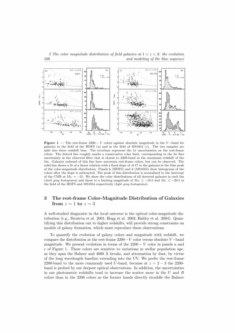
Figure 1 — The rest-fram e 220 0 − V colors ag ainst absolute m ag nitude in the V −band forg alax ies in the field of the H D F S (a) and in the field of MS 10 54 (c). The two sam ples aresplit into three redshift bins. The errorbars represent the 1σ uncertainties on the rest-fram ecolors. The dotted line roug hly m ark s a conservative color lim it, corresponding to the 2σ fl uxuncertainty in the observed filter that is c losest to 220 0 -band at the m ax im um redshift of thebin. G alax ies redward of this line have uncertain rest-fram e colors, but can be observed. Thesolid line shows a fit of a linear relation with a fix ed slope of -0 .17 to the g alax ies in the blue peakof the color-m ag nitude distribution. Panels b (H D F S ) and d (MS 10 54 ) show histog ram s of thecolors after the slope is subtracted. The peak of this distribution is norm alized to the interceptof the C MR at MV = −21. We show the color distributions of all detected g alax ies in each bin(d ark gray h istogram s) and those to a lim iting m ag nitude of MV ≤ −19 .5 and MV ≤ −20 .5 inthe field of the H D F S and MS 10 54 respectively (ligh t gray h istogram s).

3 T h e re st-fra m e C o lo r-M a g n itu d e D istrib u tio n o f G a la x ie s

fro m z ∼ 1 to z ∼ 3

A well-stu d ied d iag n ostic in the local u n iverse is the optical color-mag n itu d e d is-tribu tion (e.g ., S trateva et al. 2001; H og g et al. 2002; B ald ry et al. 2004 ). Q u an -tifyin g this d istribu tion ou t to hig her red shifts, will provid e stron g con strain ts onmod els of g alax y formation , which mu st reprod u ce these observation s.

To q u an tify the evolu tion of g alax y colors an d mag n itu d e with red shift, wecompare the d istribu tion at the rest-frame 2200−V color versu s absolu te V −ban dmag n itu d e. We presen t evolu tion in terms of the 2200 − V color in pan els a an dc of F ig u re 1. These colors are sen sitive to variation s in stellar popu lation ag e,as they span the B almer an d 4 000 A break s, an d atten u ation by d u st, by virtu eof the lon g wavelen g th baselin e ex ten d in g in to the U V . We prefer the rest-frame2200-ban d to the more common ly u sed U -ban d , becau se at z = 2 − 3 the 2200-ban d is probed by ou r d eepest optical observation s. In ad d ition , the u n certain tiesin ou r photometric red shifts ten d to in crease the scatter more in the U an d B

colors than in the 2200 colors as the former ban d s d irectly strad d le the B almer

5.4 The C olor-M agnitude Relation of B lue F ield G alaxies 109

and 4000 A breaks.

We divide the galaxies in three redshift bins centered at z=1.0, 1.8, and z=2.7 .The redshift range is defi ned so that the rest-frame 2200 and V -band always lieswithin the range of our observed fi lters. The number of redshift bins is a com-promise between keeping a statistically meaningful sample at each redshift, whilereducing the eff ects of evolution over the time span in each bin. The limits ofthe bins are defi ned so that galaxies in the smaller fi eld of the HD FS are equallydivided in number. The redshift bins of the larger M S105 4 fi eld are matched tothose of the HD FS.

C learly, in both fi elds and in all redshift bins there is a well-defi ned ridge ofblue galaxies. Furthermore, the ridge is tilted: the more luminous galaxies alongthe ridge tend to have redder 2200−V colors. This ridge is what we defi ne as thecolor magnitude relation of blue galaxies.

There is no reason to think that this color-magnitude relation is due to someselection eff ect; we can easily detect galaxies that are bright in MV and blue in2200 − V , and our photometry is suffi ciently deep to ensure that the trend is notcaused by a lack of faint red galaxies. O nly at at low redshifts (z ∼ 1) and faintmagnitudes may we miss some of the bluest galaxies, as the sample was selectedthe observed Ks-fi lter, which is signifi cantly redder than the redshifted V −bandat z ∼ 1.

It is striking that the blue color magnitude relation has a very well- defi nedboundary to the blue, and a much more extended tail to the red. This red tailextends up to 4 magnitudes, and defi nes a clear red color magnitude relation inthe lowest redshift bin in the M S105 4 fi eld. This is mainly caused by the color-magnitude relation of the cluster galaxies at z = 0.83, and is also observed in thefi eld up to z = 1 (e.g., Bell et al. 2004a)

We now proceed to analyze the properties of the blue color magnitude in sec-tions 4 and 5 , and will turn to the red galaxies in section 6 .

4 The Color-Magnitude R elation of B lue F ield Galaxies

Two key features of the blue C M R in Fig. 1 are that the peak of the distribution,and hence the zeropoint of the blue sequence, reddens from z ∼ 3 to z ∼ 1, while onfi rst sight the slope does not seem to vary appreciably. We proceed by quantifyingthe slope and zeropoint of the relation and their evolution with redshift.

4.1 T h e S lo p e a n d its E v o lu tio n

We assume that the distribution of colors and magnitudes can be characterizedby a linear relation. We obtain the best fi tting slope as follows: for each valueof the slope we obtain a distribution of color residuals. We select the slope thatmaximizes the peak of the histogram of the residuals. This so-called “mode re-



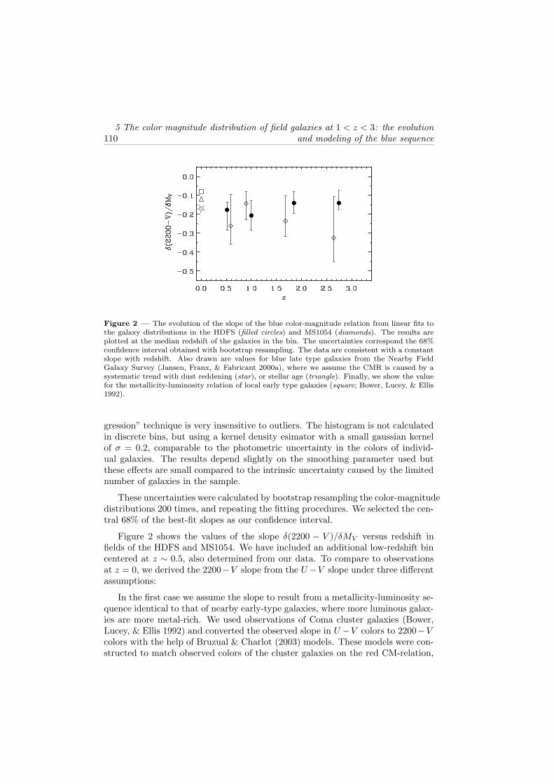
Figure 2 — The evolution of the slope of the blue color-magnitude relation from linear fits tothe galaxy distributions in the HDFS (filled circles) and MS1054 (diamon ds). The results areplotted at the median redshift of the galaxies in the bin. The uncertainties correspond the 6 8 %confidence interval obtained with bootstrap resampling. The data are consistent with a constantslope with redshift. A lso drawn are values for blue late type galaxies from the N earby FieldGalaxy Survey (J ansen, Franx, & Fabricant 2000a), where we assume the CMR is caused by asystematic trend with dust reddening (star), or stellar age (trian gle). Finally, we show the valuefor the metallicity-luminosity relation of local early type galaxies (squ are; B ower, L ucey, & E llis1992).

gression” technique is very insensitive to outliers. The histogram is not calculatedin discrete bins, but using a kernel density esimator with a small gaussian kernelof σ = 0.2, comparable to the photometric uncertainty in the colors of individ-ual galaxies. The results depend slightly on the smoothing parameter used butthese effects are small compared to the intrinsic uncertainty caused by the limitednumber of galaxies in the sample.

These uncertainties were calculated by bootstrap resampling the color-magnitudedistributions 200 times, and repeating the fitting procedures. We selected the cen-tral 68% of the best-fit slopes as our confidence interval.

Figure 2 shows the values of the slope δ(2200 − V )/ δMV versus redshift infields of the HDFS and MS1054. We have included an additional low-redshift bincentered at z ∼ 0.5, also determined from our data. To compare to observationsat z = 0, we derived the 2200−V slope from the U −V slope under three differentassumptions:

In the first case we assume the slope to result from a metallicity-luminosity se-quence identical to that of nearby early-type galaxies, where more luminous galax-ies are more metal-rich. We used observations of Coma cluster galaxies (Bower,L ucey, & E llis 1992) and converted the observed slope in U −V colors to 2200−Vcolors with the help of Bruzual & Charlot (2003) models. These models were con-structed to match observed colors of the cluster galaxies on the red CM-relation,

5.4 The Color-Magnitude Relation of Blue Field Galaxies 111

Figure 3 — The relation between 2200 − V and U − V colors for Bruzual & Charlot(2003)stellar population models with declining star formation rates and a range of timescales τ . Solarmetallicity (solid lines) and 1/3 solar models (dashed lines) are shown. The sq uare indicates stel-lar ages of ∼1 Gyr, the diamonds indicate ages of ∼10 Gyr. O ver a range of stellar populationages and metallicities the relationship is tight for blue galaxies, allowing a fairly accurate trans-formation of their colors. Also drawn is a Calzetti et al. (2000) attenuation vector of AV = 1. Inthe presence of dust, the transformation of U − V to 2200 − V colors is done with stellar tracksthat already include reddening.

assuming the expected star formation history, i.e., high formation redshift andpassive evolution.

The other two are derived from a linear fit to the U − V colors of nearbyblue-sequence galaxies from the N earby Field G alaxy Survey (N G FS; J ansen etal. 2000a). Here we synthesized the 2200−V slope under two assumptions. First,we assumed the CMR to refl ect a systematic age trend, where higher-luminositygalaxies have higher stellar ages, and we used Bruzual & Charlot (2003) modelsto transform U −V colors to 2200−V colors (see Figure 3) For galaxies with bluecolors, the models give ∆ (2200−V ) ≈ 1.5∆ (U −V ) for a range of metallicities andstellar ages. Second, we assume the slope is the result of increasing dust opacitywith luminosity. Adopting the Calzetti et al. (2000) dust law yields ∆ (2200−V ) ≈2.3∆ (U − V ). An SMC extinction law (G ordon et al. 2003) would yield similarvalues.

Fig. 2 shows that the slope of the CM relation does not depend on redshift.



Only if we use the z = 0 slope derived for very red early-type galaxies in Comais there any hint of evolution. This model is rather extreme, however, and willnot be considered further. The measured evolution of the slope is 0.01z ± 0.03,consistent with zero. The error-weigthed mean value of all FIRES measurementsis

δ(2200 − V )/δMV = −0.17 ± 0.021

If the slope were due to an age gradient as a function of magnitude, one mightexpect the slope to steepen with redshift, but we see no significant effect in thedata presented here. We analyze the cause of the relation later in §4.3.

We note that Barmby et al. (2004) found a linear CMR for faint galaxies, andan upturn of the CMR at bright magnitudes. Figure 1 shows some evidence for anupturn at the bright end, but obviously our sample is too small to describe thisproperly, and we hence focus entirely on the linear part of the relation.

4.2 The Z eropoint and its Evolution

We determine the zeropoint by assuming that the slope of the CMR does notevolve and remains at the mean value of δ(2200−V )/δMV = −0.17. We subtractthe slope so that all galaxy colors are normalized to the color at MV = −21.The histogram of normalized colors was determined as described before, and thezeropoint was determined from the location of the peak.

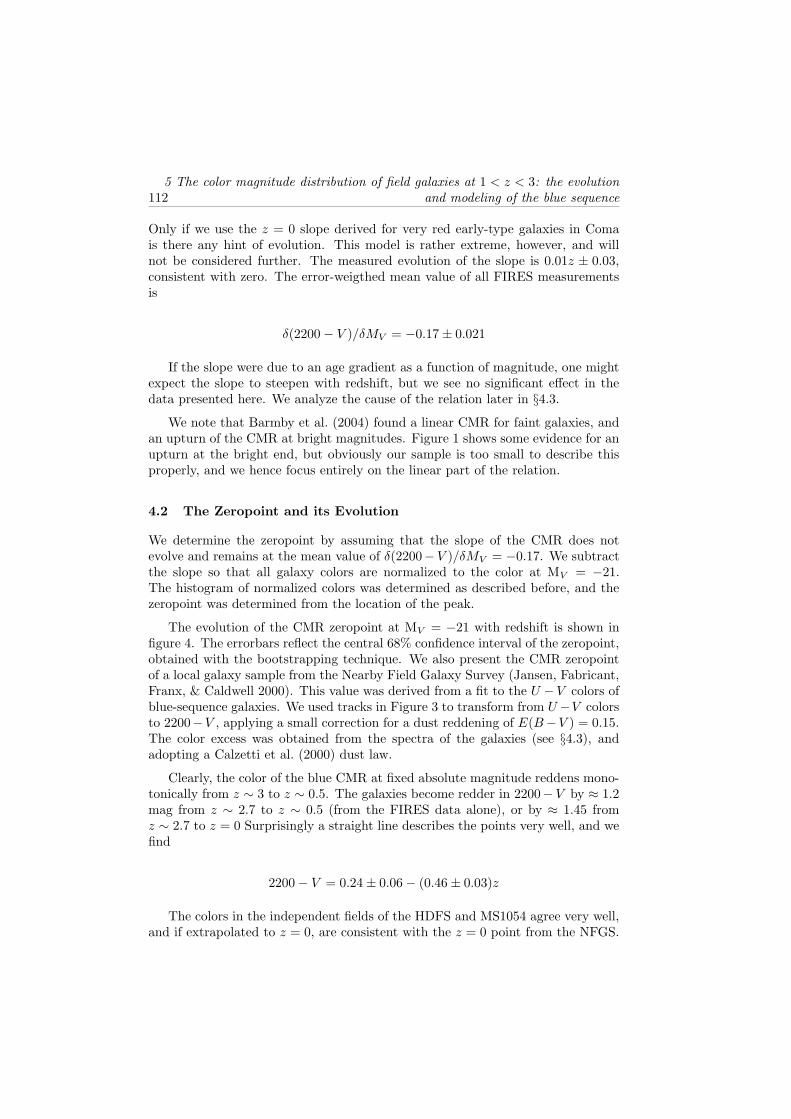
The evolution of the CMR zeropoint at MV = −21 with redshift is shown infigure 4. The errorbars reflect the central 68% confidence interval of the zeropoint,obtained with the bootstrapping technique. We also present the CMR zeropointof a local galaxy sample from the Nearby Field Galaxy Survey (Jansen, Fabricant,Franx, & Caldwell 2000). This value was derived from a fit to the U − V colors ofblue-sequence galaxies. We used tracks in Figure 3 to transform from U −V colorsto 2200−V , applying a small correction for a dust reddening of E(B−V ) = 0.15.The color excess was obtained from the spectra of the galaxies (see §4.3), andadopting a Calzetti et al. (2000) dust law.

Clearly, the color of the blue CMR at fixed absolute magnitude reddens mono-tonically from z ∼ 3 to z ∼ 0.5. The galaxies become redder in 2200−V by ≈ 1.2mag from z ∼ 2.7 to z ∼ 0.5 (from the FIRES data alone), or by ≈ 1.45 fromz ∼ 2.7 to z = 0 Surprisingly a straight line describes the points very well, and wefind

2200 − V = 0.24 ± 0.06 − (0.46 ± 0.03)z

The colors in the independent fields of the HDFS and MS1054 agree very well,and if extrapolated to z = 0, are consistent with the z = 0 point from the NFGS.


Figure 4 — The intercepts of fits to the blue CMR at fixed MV = −21, marking the colorevolution of the blue sequence as a function of redshift. We show the results in the field of theHDFS field (filled circles) and in the field of MS1054 (diamonds). The errorbars correspond to the68% confidence interval derived from bootstrap resampling. The star indicates the z = 0 relationfrom the NFGS (Jansen, Franx, & Fabricant 2000a). The lines represent tracks of Bruzual &Charlot (2003) stellar population models. We show a model with formation redshift zf = 3.2,a star formation timescale τ = 10 Gyr, and fixed reddening of E(B − V ) = 0.15 (dashed line);one with zf = 10, constant star formation, and fixed E(B −V ) = 0.15 (solid line); a model withzf = 10, τ = 10 Gyr, and E(B − V ) evolving linearly in time from 0 at z = 10 to 0.15 at z = 0(dotted line).

This is encouraging considering that absolute calibration between such differentsurveys is difficult, and that the NFGS data has been transformed to 2200 − Vcolors from other passbands.

Next we compare the observed color evolution to predictions from simple stellarpopulations models. We assume that the galaxies remain on the ridge of the CMRthroughout their life. This assumption may very well be wrong, but more extensivemodeling is beyond the scope of this paper. Obviously for such simple models,the galaxies have all the same color, and these follow directly from the colors ofthe stellar population model, depending on star formation history, and the dustabsorption only.

We calculate rest-frame colors using Bruzual & Charlot (2003) stellar pop-ulation synthesis models with solar metallicity and exponentially declining starformation rates. We added dust reddening to the model colors using a Calzetti etal. (2000) dust law. To generate colors at constant absolute magnitude we applya small color correction to account for V −band luminosity evolution of the stellarpopulation. It reflects the fact that galaxies that were brighter in the past popu-lated a different, redder part of the CMR. Similarly, when we allow varying levels



of dust attenuation, we apply a correction to account for dimming of the V -bandlight. We use the measured slope to apply the correction, the total amplitude ofthe effect is less than ∆(2200 − V ) . 0.1 for most models.

The simple model tracks are shown in Figure 4. A model with constant starformation and formation redshift zf = 10 fits remarkably bad: the evolution ismuch slower than the observed evolution. When we explore models with exponen-tially declining star formation rates, we find that a decline time scale τ = 10G y rand formation redshift zf = 3.2 fits best. We note that we restricted the fit tozf ≥ 3.2 as the color-magnitude relation is already in place at redshifts lower thanthat.

Naturally, the models can be made to fit perfectly by allowing variable redden-ing by dust. As an example we show a τ = 10 Gyr model with formation redshiftzf = 10 with reddening evolving linearly with time from E(B−V ) = 0 at zf = 10to E(B − V ) = 0.15 at z = 0.

We conclude that the relatively strong color evolution in the interval 0 < z < 3is likely caused by both aging of the stellar population and increasing levels ofdust attenuation with time.

4.3 The O rig in of the B lue Seq uence in the L ocal U niverse

It is impossible to determine the cause of the color-magnitude relation of bluegalaxies from broad band photometry alone. Fits of models to the photometryproduce age and dust estimates which are very uncertain (e.g., Shapley et al.2001, Papovich et al. 2001, Forster-Schreiber et al. 2004). Spectroscopy is neededfor more direct estimates of the reddening and ages. Unfortunately, the restframeoptical spectroscopy of distant galaxies is generally not deep enough for the de-tection of Hβ, and the balmer decrement cannot be determined to high enoughaccuracy. Hence we can only analyze the relation for nearby galaxies which havespectroscopy with high signal-to-noise ratio.

We use the local sample of galaxies in the Nearby Field Galaxy Survey (Jansen,Fabricant, Franx, & Caldwell 2000; Jansen, Franx, Fabricant, & Caldwell 2000),a spectrophotometric survey of a subsample of 196 galaxies in the CfA redshiftsurvey (Huchra et al 1993). It was carefully selected from ∼ 2400 galaxies toclosely match the distributions of morphology and magnitude of the nearby galaxypopulation, and covers a large range of magnitudes −15 < MB < −23 . Thestrength of the NFGS is the simultaneous availability of integrated broadbandphotometry, and integrated spectrophotometry of all galaxies, including line fluxesand equivalent widths of [OII] Hα, and Hβ . Integrated spectra and photometryare essential to enable a fair comparison to the integrated photometry of our high-redsfhift galaxy sample.

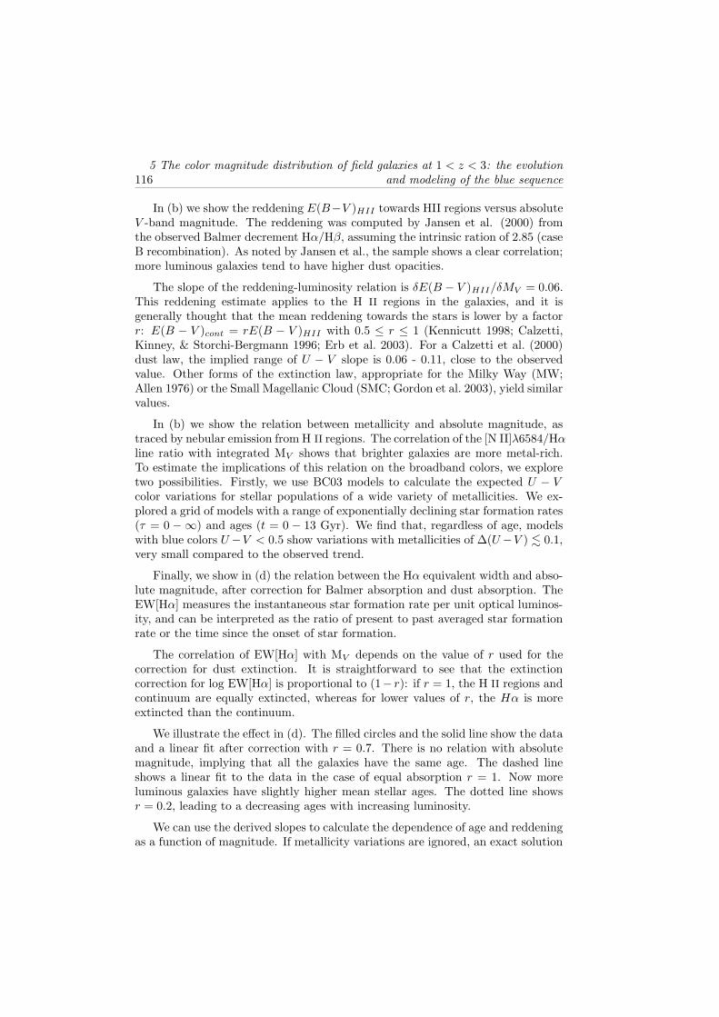
The trends of U − V colors, dust absorption, metallicity, and Hα equivalentwidth for normal nearby galaxies are illustrated in Figure 5. The distribution


Figure 5 — U −V colors and nebular emission lines properties versus absolute V -band magni-tude of nearby normal galaxies from the Nearby Field Galaxy Survey (Jansen et al. 2000a). (a)The U − V color versus absolute V magnitude. A linear fit to the blue sequence is shown (solidline). In the other panels we plot only the galaxies that are within 0.25 mag of the blue color-magnitude rellation (dashed lines). (b) The E(B − V )HII color excess versus absolute V -bandmagnitude, derived from the observed ratio of integrated fluxes of Hα and Hβ. The fluxes arecorrected for Balmer absorption and Galactic reddening. The line shows a linear fit to the data(d). The metallicity sensitive [N II]λ6584/Hα ratio. The dashed line indicates Solar metallicity.(c) The Hα equivalent width EW[Hα], corrected for Balmer absorption and attenuation by dust.The correction for dust absorption was obtained from the measured E(B −V )HII and assumingan absorption of the stellar continuum E(B − V )c o n t = rE(B − V )HII , where r = 0.7. Thesolid line is a linear fit to the data. Also shown are linear fits to the data in the case that r = 1(dashed line) and r = 0.2 (dotted line).

U − V colors versus absolute V magnitudes is shown in (a). A blue sequence anda red sequence of galaxies are visible. A linear fit to the blue sequence using thesame technique as described in §4.1 gives a slope of δ(U − V )/δMV = −0.08. Weisolate the blue galaxies and only consider the spectral properties of galaxies withcolors ∆(U − V ) < 0.25 from the linear fit.



In (b) we show the reddening E(B−V )HII towards HII regions versus absoluteV -band magnitude. The reddening was computed by Jansen et al. (2000) fromthe observed Balmer decrement Hα/ Hβ, assuming the intrinsic ration of 2.85 (caseB recombination). As noted by Jansen et al., the sample shows a clear correlation;more luminous galaxies tend to have higher dust opacities.

The slope of the reddening-luminosity relation is δE(B − V )HII/δMV = 0.06.This reddening estimate applies to the H II regions in the galaxies, and it isgenerally thought that the mean reddening towards the stars is lower by a factorr: E(B − V )c o n t = rE(B − V )HII with 0.5 ≤ r ≤ 1 (K ennicutt 1998; Calzetti,K inney, & Storchi-Bergmann 1996; Erb et al. 2003). For a Calzetti et al. (2000)dust law, the implied range of U − V slope is 0.06 - 0.11, close to the observedvalue. Other forms of the extinction law, appropriate for the Milky Way (MW;Allen 1976) or the Small Magellanic Cloud (SMC; Gordon et al. 2003), yield similarvalues.

In (b) we show the relation between metallicity and absolute magnitude, astraced by nebular emission from H II regions. The correlation of the [N II]λ6584/Hαline ratio with integrated MV shows that brighter galaxies are more metal-rich.To estimate the implications of this relation on the broadband colors, we exploretwo possibilities. Firstly, we use BC03 models to calculate the expected U − Vcolor variations for stellar populations of a wide variety of metallicities. We ex-plored a grid of models with a range of exponentially declining star formation rates(τ = 0 −∞) and ages (t = 0 − 13 Gyr). We find that, regardless of age, modelswith blue colors U −V < 0.5 show variations with metallicities of ∆(U −V ) . 0.1,very small compared to the observed trend.

Finally, we show in (d) the relation between the Hα equivalent width and abso-lute magnitude, after correction for Balmer absorption and dust absorption. TheEW[Hα] measures the instantaneous star formation rate per unit optical luminos-ity, and can be interpreted as the ratio of present to past averaged star formationrate or the time since the onset of star formation.

The correlation of EW[Hα] with MV depends on the value of r used for thecorrection for dust extinction. It is straightforward to see that the extinctioncorrection for log EW[Hα] is proportional to (1− r): if r = 1, the H II regions andcontinuum are equally extincted, whereas for lower values of r, the Hα is moreextincted than the continuum.

We illustrate the effect in (d). The filled circles and the solid line show the dataand a linear fit after correction with r = 0.7. There is no relation with absolutemagnitude, implying that all the galaxies have the same age. The dashed lineshows a linear fit to the data in the case of equal absorption r = 1. Now moreluminous galaxies have slightly higher mean stellar ages. The dotted line showsr = 0.2, leading to a decreasing ages with increasing luminosity.

We can use the derived slopes to calculate the dependence of age and reddeningas a function of magnitude. If metallicity variations are ignored, an exact solution


can be derived: The reddening of the H II regions follows immediately from thedata, r and the slope of log age versus magnitude follow directly from the observedslopes of U −V versu s m ag n itu d e an d E W[H α] versu s m ag n itu d e. T h e solu tion is

r = 0.7 8

an d

δ log (a g e)/ δMV = 0.027

T h is ag e g rad ien t is very sm all, an d prod u ces a very sh allow color m ag n itu d eslope of 0.01, opposite to th e observed slope. T h e m ain cau se of th e color m ag -n itu d e relation is th e variation of d u st red d en in g with m ag n itu d e. T h ese resu ltsd oes n ot ch an g e sig n ifi can tly if m etallicity con tribu tes -0.01 to th e color m ag n itu d erelation .

We con clu d e th at th e d ata on local g alax ies im ply th at th e C MR for blu eg alax ies is m ostly cau sed by variation s in red d en in g , with on ly sm all con tribu tion sfrom ag e an d m etallicity variation s.

4.4 C o m p a riso n to z ∼ 3 G a la x ie s

We tu rn to ou r broad ban d observation s at z ∼ 3 an d com pare th e situ ation in th elocal u n iverse to th at at h ig h red sh ift. We select th e 18 6 g alax ies in th e FIR E Ssam ple at 2.2 < z < 3.2, an d in spect th e properties of th e g alax ies th at lie with in∆ (2200 − V ) < 1 m ag of th e blu e C MR .

4.4.1 T h e M o d e ls

Followin g previou s stu d ies of h ig h red sh ift g alax ies (Papovich , D ick in son , & Fer-g u son 2001; S h apley et al. 2001; Forster S ch reiber et al. 2004 ), we fi t stellar pop-u lation m od els to th e broad ban d S E D s of in d ivid u al g alax ies, an d in terpret th ed istribu tion of best-fi t ag es an d ex tin ction s. We u se th e pu blicly availably H Y -PE R Z fi ttin g cod e (B olzon ella, Miralles, & Pello 2000), u pd ated with th e syn th etictem plate spectra from th e latest version of th e B ru z u al & C h arlot (2003) stellarpopu lation syn th esis cod e. We u se th e B asel 3.1 library (Westera et al. 2002) ofth eoretical stellar spectra, selected th e Pad ova19 9 4 stellar evolu tion ary track s, an dad opted a S alpeter IMF with u pper an d lower m ass cu t-off s of 0.1 an d 100 M¯.

For sim plicity, we on ly d iscu ss th e resu lts for m od els with con stan t star form a-tion rates an d solar m etallicity. Metallicities of blu e, star-form in g g alax ies z ∼ 2−3are n ot well con strain ed ,an d m ay be solar (S h apley et al. 2004 ) or som ewh at lower(Pettin i et al. 2001). We prefer solar m etallicity m od els as th ey h ave been d irectlycalibrated ag ain st em pirical stellar spectra. We refer to earlier stu d ies for d etailedd iscu ssion s h ow th e m od el assu m ption s aff ect th e d istribu tion of best-fi t param -eters Papovich , D ick in son , & Ferg u son (2001); S h apley et al. (2001). Fin ally, we



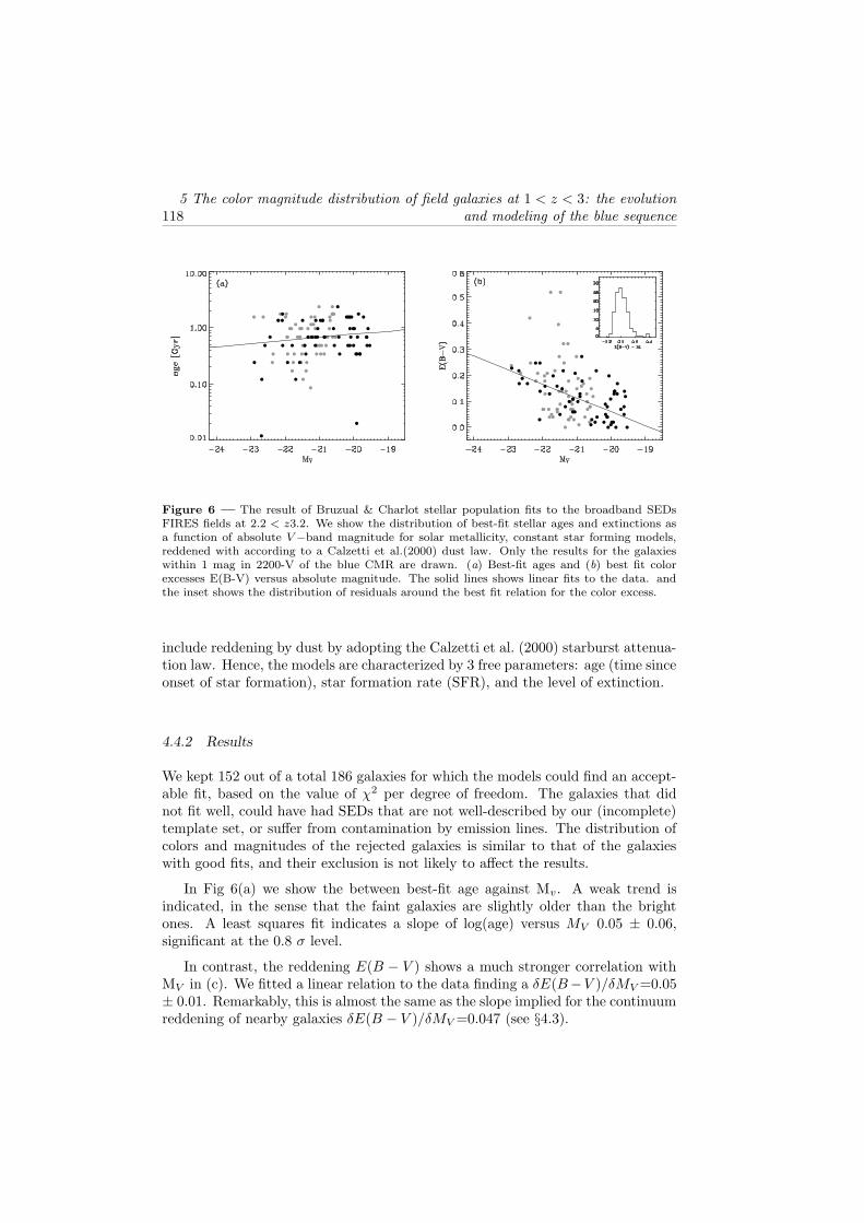
Figure 6 — The resu lt o f B ru z u al & C harlo t stellar po pu latio n fi ts to the bro ad ban d S E D sF IR E S fi eld s at 2.2 < z3.2. We show the d istribu tio n o f best-fi t stellar ag es an d ex tin c tio n s asa fu n c tio n o f abso lu te V −ban d m ag n itu d e fo r so lar m etallic ity, c o n stan t star fo rm in g m o d els,red d en ed with acc o rd in g to a C alzetti et al.(20 0 0 ) d u st law. O n ly the resu lts fo r the g alax ieswithin 1 m ag in 220 0 -V o f the blu e C M R are d rawn . (a) B est-fi t ag es an d (b) best fi t c o lo rex cesses E (B -V ) versu s abso lu te m ag n itu d e. The so lid lin es shows lin ear fi ts to the d ata. an dthe in set shows the d istribu tio n o f resid u als aro u n d the best fi t relatio n fo r the c o lo r ex cess.

include reddening by dust by adopting the Calzetti et al. (2000) starburst attenua-tion law. Hence, the models are characterized by 3 free parameters: age (time sinceonset of star formation), star formation rate (SFR), and the level of extinction.

4.4.2 R esu lts

We kept 15 2 out of a total 186 galaxies for which the models could find an accept-able fit, based on the value of χ2 per degree of freedom. The galaxies that didnot fit well, could have had SEDs that are not well-described by our (incomplete)template set, or suffer from contamination by emission lines. The distribution ofcolors and magnitudes of the rejected galaxies is similar to that of the galaxieswith good fits, and their exclusion is not likely to affect the results.

In Fig 6(a) we show the between best-fit age against Mv. A weak trend isindicated, in the sense that the faint galaxies are slightly older than the brightones. A least sq uares fit indicates a slope of log(age) versus MV 0.05 ± 0.06,significant at the 0.8 σ level.

In contrast, the reddening E(B − V ) shows a much stronger correlation withMV in (c). We fitted a linear relation to the data finding a δE(B−V )/δMV =0.05± 0.01. Remarkably, this is almost the same as the slope implied for the continuumreddening of nearby galaxies δE(B − V )/δMV =0.047 (see §4.3).

5.4 The C olor-M agnitude Relation of B lue F ield G alaxies 119

Figure 7 — The steepness of the CMR slope versus wavelength in the field of the H DFS.The data show the slope in the rest-frame λ − V color versus MV as a function of the filterλ. Overplotted are expectations for three extinction laws: the Calzetti et al. (2000) dust law(dashed lin e), the MW extinction law (A llen 19 7 6 ; do tted), and the SMC extinction law (G ordonet al. (2003); dash-do t lin e). The normalization is diff erent for each law: δE(B −V )/ δMV = 0.04for the Calzetti, 0.05 for the MW, and 0.02 for the SMC. The thick solid line represents thecolor-dependence of the CMR slope in the case that stellar population age correlates with MV .We show the track for a solar-metallicity, constant star-forming model. The normalization islog(age) ∝ −0.30 MV .

4.4.3 The B lue C MR in Va rious Rest-F ra m e C olors

As another way to show why the data imply dust as the main cause of the CMRslope, we derived the slope of the CMR for many different restframe filters, andshow the results in Figure 7. We described our rest-frame luminosities and colorsearlier in §2.2. We overplot the expected relation as a function of wavelength forseveral extinction curves. These curves were scaled with an arbitrary constant toprovide the best fit. As we can see, the Calzetti curve provides the best fit, whereasthe SMC and MW curve fit progressively worse. We also show the expecteddependence if the CMR is caused by age variations. Again, the amplitude of thiscurve is fitted to the data points. It does not fit at all to the bluest point, whichis the CMR slope in 1400 − V color versus MV .

We conclude that, models fits to SEDs at z = 3 are in agreement with thepicture in local universe. Reddening by dust explaines the slope of the CMRconsistently.



5 C o n stra in ts o f th e C o lo r-M a g n itu d e R e la tio n o n th e

S ta r Fo rm a tio n H isto rie s o f B lu e G a la x ie s a t z ∼ 3

In this section we explore models to produce the narrow and asymmetric colordistribution of galaxies along the CMR. We focus on the redshift range 2.2 <z < 3.2, where the fraction of red galaxies is the lowest, and where perhaps thecolor distribution may be described by simpler models than at lower redshift. Thedistribution (Figure 1) is characterized by a blue peak and a skewness to muchredder colors. The color distribution has a sharp cutoff at the blue side of thepeak, and the scatter of the colors around the peak is quite low: most of the highredshift galaxies occupy a narrow locus in color space.

Here, our basic assumption is that the color scatter around the CMR is causedby age variations. We explore 4 different scenarios. In each scenario, we generatethe complete star formation history of model galaxies, typically characterized by2 or 3 free parameters. We then compile a large library of Monte-Carlo realiza-tions, and generate the expected galaxy color distributions, taking into accountobservational errors and biases. We compare the model distributions to the ob-served color distribution to identify the best fitting parameterizations of the starformation histories. K auffmann et al. (2003) used a similar method to constrainthe star formation histories of local galaxies from the Sloan Digital Sky Survey.

A desirable property of this method, as will become apparent below, is that byusing the information contained in the galaxy color distribution, we can resolvesome of the degeneracies produced by fitting SEDs to the broadband colors ofindividual galaxies (e.g., Papovich, Dickinson, & Ferguson 2001), in particular thedegeneracies in prior star formation history.

With this in mind, we will now discuss the model ingredients, the generationof the library, the fitting methodology, and the results for several different param-eterizations of the star formation histories.

5.1 A lib rary of S tar Formation H istories

As the basic ingredient, we used the solar metallicy BC03 models as discussed in§4.4, and we fixed the BC03 model parameters except the star formation history:we only explore the effect of aging on the galaxy color distributions. We willcompare the predictions of the models directly to our rest-frame luminosities andcolors (see §2.2).

We generated a large library of Monte-Carlo realizations of stellar populationswith different star formation histories. We classify the formation histories into 4seperate scenarios, characterized by distinct parameterizations of the star forma-tion rates. They range from simple constant star formation, to complex modelsincluding bursts. Details of the parameterizations are given together with the re-sults in §5.3. We do not introduce additional complexity, such as a distribution ofmetallicities, or distributions in the star formation rate parameters, as we do not

5.5 Constraints of the Color-Magnitude Relation on the

S tar Formation H istories of Blue Galaxies at z ∼ 3 121

have suffi cient observational constraints to justify more freedom in the models.

For each scenario, and for each SFH parameter combination, we generated be-tween 100-200 realizations of individual star formation histories. For every instancewe saved a selection of parameters, including colors, magnitudes, star formationrates, and masses. The final libraries of the scenarios contain on the order of ∼ 105

unique star formation histories each.

5.2 Fitting M eth od

Briefl y, we draw samples from the libraries, generate distributions of colors andmagnitudes, and compare them to rest-frame luminosity and colors of FIRESgalaxies in the redshift range 2.2 < z < 3.2. We fit the models seperately to thecolor distributions of the HDFS and MS1054 fields, as these have different depthsand areas.

5.2.1 Creating Mock O b serv ations

We need to account for three essential aspects of the data: the observations aremagnitude limited, contain photometric errors, and have additional color scatterby variations in dust content.

It is evident that magnitude limits can substantially alter the resulting colordistribution if galaxies in the models evolve strongly in luminosity. For example,an otherwise undetected galaxy undergoing a massive burst will temporarily in-crease in luminosity, and can enter a magnitude-limited sample, changing the colordistribution. This effect is enhanced if there are many more galaxies below themagnitude limit than above. Hence, the steepness of the faint end slope of theluminosity function also plays a role.

We adopt a faint-end slope of α = −1.6 according to the rest-frame far-UVluminosity function of Steidel et al. (1999). Shapley et al. (2001) found a steeperslope, but it resulted from a positive correlation of observed R and R − Ks pho-tometry, which we do not see in our data. We applied the luminosity function inthe following way.

From the models we generate sets of galaxies with the same redshift distributionas the observed distribution. We then draw a luminosity from a luminosity functionwith α = −1.6 and scale the model galaxy to that luminosity. Instead of using theinstantaneous luminosity of the mock galaxy at the time of observation to computethe scaling, we use its median luminosity over the redshift range 2.2 < z < 3.2.

Furthermore, we add photometric errors to the model colors as a function ofmodel luminosity. The standard deviations of the errors were determined from alinear fit to the errors on the rest-frame luminosities and colors as a function ofrest-frame MV . Hence, these include the photometric redshift uncertainties. Thefit gives a mean error in the rest-frame 2200 − V color of 0.15 in the HDFS and



0.19 for the MS1054.

Finally, we include reddening by dust in the models, adopting the Calzetti etal. (2000) starburst attenuation law. We add a distribution of color excesses

E(B − V ) = 0.1 ± 0.05(1σ)

to the model colors and magnitudes, where E(B −V ) is required to be greaterthan 0. The mean value is appropriate for MV = −21 galaxies from the best-fit models in §4.3, and we used a scatter of 0.05 equal to that found in localgalaxies (see §4.2) and similar to the distribution of E(B − V ) in §4.3. U singthis distribution of extinctions, the scatter added to the model colors is σ(2200 −

V )d u st ∼ 0.2. Adopting an SMC extinction law would result in σ(2200−V )d u st ∼

0.15. We remark that the extinction variations of the FIRES galaxies at z = 2− 3are well-constrained by the low scatter in the rest-frame far-U V colors.

Summing up, the average (2200 − V ) scatter introduced into the models byincluding both photometric uncertainties and dust variations is 0.25 mag for theHDFS, and 0.28 mag for the MS1054 field. N ote that the width of the observedscatter at 2.2 < z < 3.2, which we characterize by the central 32% of the colordistribution, is 0.58 and 0.83 (for the HDFS and MS1054, respectively; see alsoTable 2).

Finally, to complete the mock color distributions, we imposed a magnitudelimit of MV = −19.5 for the HDFS field, and MV = −20.5 for the field of MS1054.We are complete for all SED types down to these magnitude limits.

5.2.2 The Fitting

First, we subtracted the color-magnitude relation δ(2200− V )/δMV from the ob-served colors as in §4.2, and we normalize the 2200 − V color distribution to thecolor of the CMR intercept at MV = −21. Then, for each scenario and for eachfield, we found the best-fit parameters by performing the two-sided Kolmogorov-Smirnov (KS) test on the unbinned color distributions of the models and the data.N ext, we multiplied the KS-test probabilities of the individual fields, and we se-lected the parameter combination that yielded the highest probability.

A property of the KS-test is that it tends to be more sensitive around themedian values of the distribution than at the extreme ends (Press et al. 1992).G iven this behaviour, it is easy to see that our assumptions for the stellar pop-ulation model, such as IMF and metallicity, may impose strong, yet undesirable,constraints on the fits. For example, a steeper IMF slope less rich in high-massstars (e.g., Scalo instead of Salpeter) results in inherently redder spectra, whereaslower metallicity of the stellar populations leads to intrinsically bluer spectra. TheKS-test would be sensitive to these systematic color changes in color, violation ourbasic assumption that the variations in color are caused by variations in age alone.


Star Formation Histories of Blue Galaxies at z ∼ 3 123

Furthermore, both the FIRES fields contain some very red galaxies (Franx etal. 2003; van Dokkum et al. 2003). These galaxies are thought to have much largerdust extinctions, higher ages, and perhaps different star formation histories thanthe z ∼ 3 blue sequence galaxies we model here (see, e.g., van Dokkum et al.2004; Forster Schreiber et al. 2004a). In principle, we do not expect our simplemodels to account for them, and while the KS-test is relatively insensitive to asmall numbers of outliers, we might consider excluding them from the fit.

For these reasons we perform 3 different KS-tests, which we will refer to asKS1, KS2, and KS3. Firstly, we do a straightforward two-sided KS-test on themodel and observed distributions. For the second, we normalize both the modeland the observed color distribution to the median, and hence we only test for theshape of the color distribution, and not the absolute value of the color. L astly,we compare the median normalized distributions after excluding galaxies that are∆(2200 − V ) > 1.75 redder than the mode of the distributions, thereby removingthe reddest outliers. The mode is calculated as in §4.1.

In the subsequent presentation of the results we focus on the second test (KS2),which is sensitive to the shape only, but we discuss the outcome of the other testswhere appropriate.

We note in advance, that due to inherent differences between the fields thecombined KS probabilities will never reach high values. For example, a two-sided KS-test comparing the MS1054 data to the observations of the HDFS (to amagnitude limit of MV = −20.5) gives a probability of 70%. We do not expectany model that fits both data sets to exceed this probability.

5.3 R esu lts

5.3.1 Constant S tar Formation

In scenario 1, we assume galaxies start forming stars at random redshifts zf . Wetake zf to be distributed uniformly in time from z = 2.2 up to a certain certainmaximum redshift zm a x , where zm a x is between 3.2 < zm a x < 10 in steps of 0.2.The star formation rate of each individual galaxy is constant for a certain timetsf after which star formation ceases. We construct predictions for values of tsf

sampled logarithmically in 10 steps from 0.05 to 3 Gyr. Hence, this model ischaracterized by two parameters: zm a x and tsf .

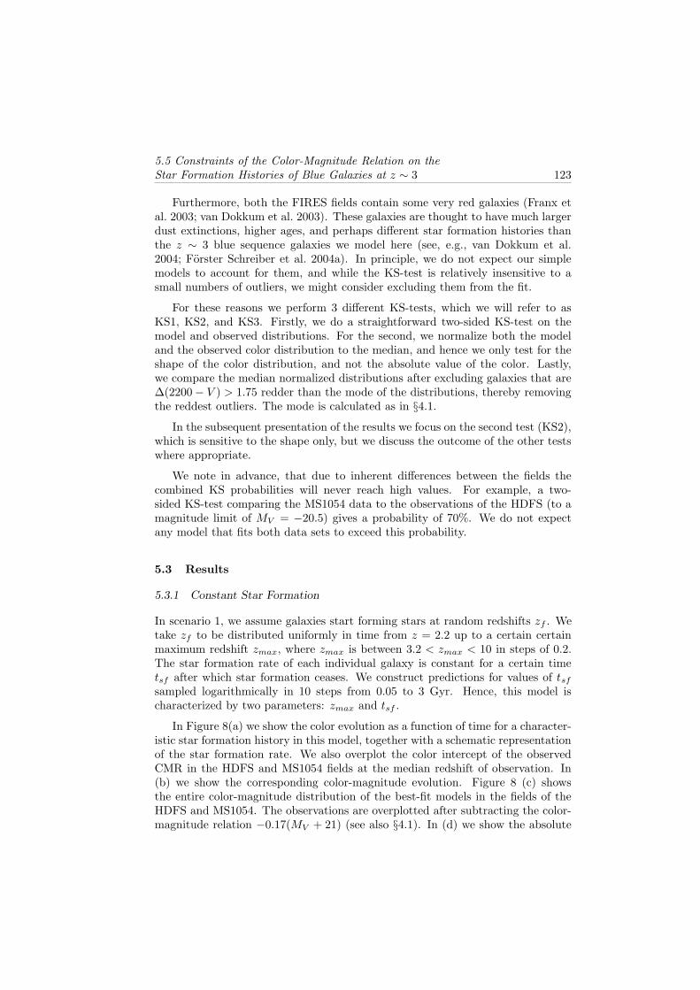
In Figure 8(a) we show the color evolution as a function of time for a character-istic star formation history in this model, together with a schematic representationof the star formation rate. We also overplot the color intercept of the observedCMR in the HDFS and MS1054 fields at the median redshift of observation. In(b) we show the corresponding color-magnitude evolution. Figure 8 (c) showsthe entire color-magnitude distribution of the best-fit models in the fields of theHDFS and MS1054. The observations are overplotted after subtracting the color-magnitude relation −0.17(MV + 21) (see also §4.1). In (d) we show the absolute



Figure 8 — The results of model 1. Galaxies in this model start off at random redshiftsz0 < zmax, an d fo rm stars at a co n stan t rate fo r a d u ratio n ts f befo re sto ppin g . T h e m ax im u mfo rm atio n red sh ift zmax an d ts f are th e free param eters. (a) T h e stellar po pu latio n track o f2200− V co lo r ag ain st ag e fo r a ch aracteristic g alax y (z0 = 4, ts f = 1 G yr). T h e star fo rm atio nrate is illu strated sch em atically by th e g ray lin e. Also d rawn is th e o bserv ed 2200 − V co lo r o fth e blu e C MR at fi x ed MV = −21 in th e H D F S (star) an d MS 105 4 (diam o n d). A m ean d u stred d en in g o f E(B − V ) = 0.1 ≈ E(2200 − V ) = 0.4 (C alzetti et al 2000) is ad d ed to th e m o d elco lo r. (b) T h e track o f 2200 − V co lo r ag ain st abso lu te V -ban d m ag n itu d e fo r th e sam e g alax yin steps o f 100 Myr (fi lled circles) (c) T h e fu ll co lo r-m ag n itu d e d iag ram o f th e best-fi t m o d el(black po in ts) in th e red sh ift ran g e 2.2 < z < 3.2. T h e fi lled g ray circles are th e d ata fro m th eH D F S (to p) an d MS 105 4 (bo tto m ). T h e co lo r d istribu tio n o f th e m o d el is bro ad en ed to acco u n tfo r ph o to m etric erro rs an d scatter in th e d u st pro perties, wh ere we u sed σ(2200− V )d u s t = 0.2.O n ly g alax ies brig h ter th an th e abso lu te m ag n itu d e cu t-o ff (dash ed lin e) are in clu d ed in th e fi t.(d) T h e h isto g ram s o f resid u al 2200 − V co lo rs sh ow th e d ata (gray h istogram s) an d th e best-fi tm o d el (h atch ed h istogram s). T h e best-fi t param eters are zmax = 4.6 an d ts f = 1 G yr.

color histog ram s of the best-fi t m od el tog ether with the d ata. We n ote that the

“ shape-sen sitiv e” K S 2 test was u sed to fi n d the best fi t.

T he best-fi t m od el in the K S 2 test has a m ax im u m form ation red shift zmax =

4.6 an d a con stan t star form ation tim escale ts f = 1 G yr. S om e characteristics are

reprod u ced , su ch as the n arrow blu e peak , bu t the asym m etric profi le in the blu e

peak is n ot, althou g h there is a low-lev el tail to red colors con tain in g passiv ely

ev olv in g g alax ies. T he fi t is rather poor; the K S 2 -test assig n s a 0 .11 probability

to the fi t, the K S 1 g iv es a m ax im u m 0 .0 1, while the K S 3 g iv es 0 .0 4.

In ord er to u n d erstan d the behav iou r of this m od el, we ex plored the zmax an d

ts f param eter space. We fou n d this m od el can n ot prod u ce the d istin ct sk ewn ess

toward s red colors in the blu e peak , ev en if it cu ts off star form ation in a su bstan tial

fraction of the g alax ies arou n d the epoch of observ ation . T his wou ld be on ly

m echan ism to prod u ce a red sk ew in this m od el, bu t the red d en in g of the passiv ely

5.5 C o n stra in ts o f th e C o lo r-M a gn itu d e Rela tio n o n th e

S ta r Fo rm a tio n H isto ries o f B lu e G a la xies a t z ∼ 3 125

Figure 9 — Same as Figure 8 for model 2. Galaxies start forming stars at random redshiftsz0 < zmax, and form stars at an exponentially declining rate with e-folding time τ . The maximumformation redshift zmax and τ are the free parameters in this model. A characteristic galaxyshown in (a,b) has z0 = 3.5 and τ = 0.5 Gyr. The best-fit parameters of the in model (c,d) arezmax = 4.2 and τ = 0.5 Gyr.

evolving galaxies is so rapid (see F ig. 8 a) that instead of a red wing, it producesa prominent second red peak of passively evolving systems.

5.3.2 E x p o n e n tia lly D e c lin in g S ta r Fo rm a tio n

Scenario 2 is almost identical to the first, but now each individual galaxy has asingle exponentially declining star formation rate with timescale τ . This model ischaracterized by two parameters: τ and zmax, where τ is sampled logarithmicallyin 10 steps from 0.05 to 3 Gyr.

F igure 9 shows a characteristic star formation history, and the fitting resultsof scenario 2. The KS2 test yields a best-fit model with a maximum formationredshift zmax = 4.2 and a constant star formation timescale τ = 0.5 Gyr. It fitsvery poorly however, as the distribution is too broad and symmetric around themedian. The KS2 test rules out this model at the 99% confidence level. The KS1and KS3 test give similar answers.

E xploring the zmax and τ parameter space, we can understand why the fit isalways poor. The only way for this model to produce a red skew in the colordistribution, is by having a relatively small value for the star formation timescaleτ compared to the mean age of the galaxies at 2.2 < z < 3.2. In that case,a substantial number of galaxies is entering a “post-starburst” phase, where the

1265 T he color magnitude distribution of fi eld galaxies at 1 < z < 3: the evolution

and modeling of the b lue sequence

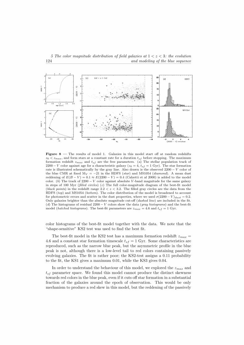
Figure 1 0 — Same as Figure 8 for model 3. Repeated burst models, with a multicompenentstar formation history: an underlying constant star formation rate, and superimposed bursts ofa certain strength r = Mburst/Mto t and freq uency n. The formation redshift is fixed to z = 10.A characteristic galaxy shown in (a,b) has n = 1 and r = 1 Gyr−1. The best-fit parameters ofthe model in (c,d) are n = 0.3 Gyr−1 and r = 4. The dashed line in (a) represents a constantstar forming model (B ruzual & Charlot 2003).

mean stellar age is t > τ and the instantaneous SFR becomes much smaller thanthe past average. These galaxies gradually move away from the blue C M R , creatinga skewness to red colors.

H owever, τ = 0.5 Gyr models redden more q uickly than C SF models at allages, as can be seen comparing Fig 9a with Fig 8a. This results in somewhatredder mean colors, and a broader spread on the blue side of the peak, created bythe newly formed galaxies that are continuously added to the sample.

5.3.3 R epeated B u rsts

In scenario 3, all galaxies start forming stars at a fixed z = 10. The stars formin two modes: a mode of underlying constant star formation, and superimposedon this, random star bursts. The bursts are distributed uniformly in time withfreq uency n: the average number of bursts per Gyr. The amplitude of the burstis parameterized as the mass fraction r = Mburst/Mto t where Mburst is the stellarmass formed in the burst and Mto t is the total mass formed by the constant starformation and any previous bursts combined. D uring a burst, stars form at aconstant, elevated rate for a fixed time tburst = 100 M yr. Thus, there are two freeparameters in this model: the burst freq uency n, and the burst strength r. Wesample n as n1/2 from 0.1 to 6 Gyr−1, and r as r1/3 from 0.01 to 4.



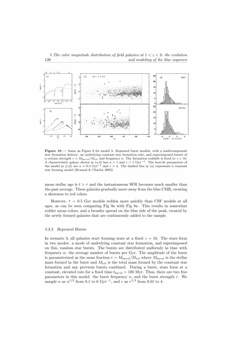
Figure 11 — The map of K S-probabilities versus model parameter repeated burst models ofscenario 3. The free parameter were the burst frequency, and the strength r = Mburst/Mtot ofthe bursts. The grayscale linearly encodes the probability of the fit. It shows the degeneraciesof the model parameters, and regions of parameter space that are clearly excluded. The panelscorrespond to the model fits to the HDFS data, MS1054 data, and the data sets combined.

Figure 10 shows a characteristic star formation history and the best-fit resultsof scenario 3. The KS2 test yields a best-fit model with an average burst frequencyof 0.3 Gyr−1 and a mass fraction formed in each burst of r = Mburst/Mtot = 4(= 400%): extremely massive, but relatively infrequent bursts. This solutionreproduces the correct shape of the color distribution, i.e., the blue cut-off and redskew, but not the absolute colors. The median 2200− V color is 0.4 mag too red,refl ecting the z = 10 formation redshift. The KS2 test probability for this modelis 0.35, with the KS3 test giving a similar value. The KS1 test rejects the modelat the 99% confidence level, as a result of the wrong median color.

We explore in Figure 11 the KS2-fit probability over the relevant part of n,rparameter space. In both fields, only models with infrequent massive bursts areallowed, although the exact strength is relatively unconstrained. There is notabledifference between the HDFS and MS1054 fields. Specifically, the broader red wingin MS1054 observations compared to the HDFS favors a higher burst frequency.

A s illustrated in Figure 10(a), the skewness towards red colors is produced bypost-starburst galaxies. These galaxies have just formed large numbers of A -starsin the previous burst that outshine for some time the O - and B -stars formed in theunderlying mode of constant star formation, hence biasing the integrated colorsto the red. Interestingly, the color of a galaxy after a starburst always remainredder compared to constant star formation (or no bursts). Concluding, recurrentbursts do not “rejuvenate” the ensemble of galaxies. Rather, after a very briefblue period during the burst, the galaxy is redder forever after.



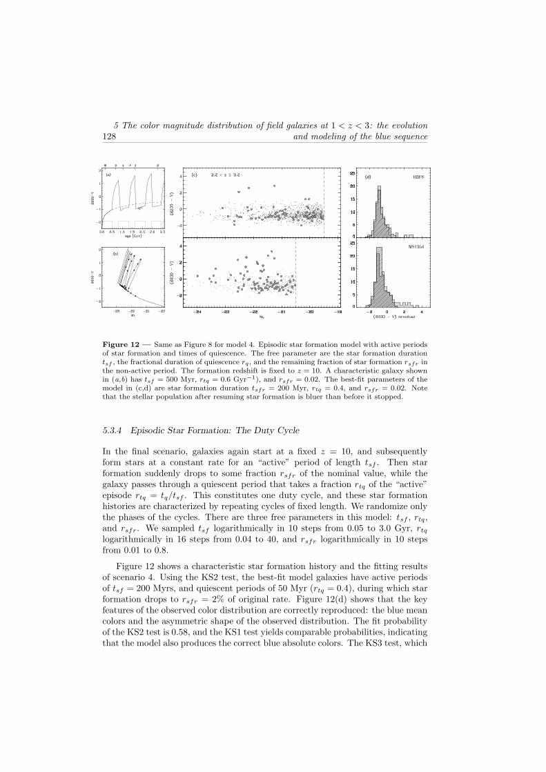
Figure 12 — Same as Figure 8 for model 4. E pisodic star formation model with active periodsof star formation and times of quiescence. The free parameter are the star formation durationtsf , the fractional duration of quiescence rq , and the remaining fraction of star formation rsfr inthe non-active period. The formation redshift is fixed to z = 10. A characteristic galaxy shownin (a,b) has tsf = 500 Myr, rtq = 0.6 Gyr−1), and rsfr = 0.02. The best-fit parameters of themodel in (c,d) are star formation duration tsfr = 200 Myr, rtq = 0.4, and rsfr = 0.02. N otethat the stellar population after resuming star formation is bluer than before it stopped.

5.3.4 Episodic Star Formation: T h e Duty C ycle

In the final scenario, galaxies again start at a fixed z = 10, and subsequentlyform stars at a constant rate for an “active” period of length tsf . Then starformation suddenly drops to some fraction rsfr of the nominal value, while thegalaxy passes through a quiescent period that takes a fraction rtq of the “active”episode rtq = tq/tsf . This constitutes one duty cycle, and these star formationhistories are characterized by repeating cycles of fixed length. We randomize onlythe phases of the cycles. There are three free parameters in this model: tsf , rtq,and rsfr. We sampled tsf logarithmically in 10 steps from 0.05 to 3.0 Gyr, rtq

logarithmically in 16 steps from 0.04 to 40, and rsfr logarithmically in 10 stepsfrom 0.01 to 0.8.

Figure 12 shows a characteristic star formation history and the fitting resultsof scenario 4. U sing the KS2 test, the best-fit model galaxies have active periodsof tsf = 200 Myrs, and quiescent periods of 50 Myr (rtq = 0.4), during which starformation drops to rsfr = 2% of original rate. Figure 12(d) shows that the keyfeatures of the observed color distribution are correctly reproduced: the blue meancolors and the asymmetric shape of the observed distribution. The fit probabilityof the KS2 test is 0.58, and the KS1 test yields comparable probabilities, indicatingthat the model also produces the correct blue absolute colors. The KS3 test, which



Figure 13 — The map of KS-probabilities versus model parameters in the duty-cycle modelsof scenario 4. The free parameter were the star formation duration tsf , the fractional durationof quiescence rq , and the remaining fraction of star formation rsfr in the non-active period. Theseven panels in each row correspond to 2-dimensional slices of the 3-dimensional parameter cube.Each slice is taken at a fixed rsfr, which is indicated in the lower-right corner. The three rowscorrespond to the model fits to the HDFS data, MS1054 data, and the data sets combined. Thegrayscale encodes linearly the probability of the fit.

excludes the reddest galaxies, yields 0.89, reflecting that the mismatch with themodel, but also between the two fields mutually, is mainly the enhanced numberof very red galaxies in the field of MS1054 (see also Forster Schreiber et al. 2004).We discussed in §5.2 that our models are not necessarily expected to describe thesmall number of very red galaxies, and we conclude that this model provides thebest description of the shape of the blue peak.

In Figure 13 we show the distribution of the (KS2) fit probabilities over theentire 3-dimensional parameter space. We present 2-dimensional slices of param-eter space at steps in fraction of residual star formation rate rsfr. The parameterspace allowed by the two datasets are somewhat different. The scatter in theHDFS is intrinsically smaller, leading to smaller values of rq and allowing longerstar formation durations tsf . Also noticable is the “plume” of reasonably highprobabilities in tsfr, rtq. This region of parameter space resembles the model dis-cussed in §5.3.1, where star formation is constant and stops exactly at the ageof observation. The broader red wing of MS1054 clearly favors longer quiescentperiods and short duty-cycles. It can also be seen that the length of the cycles isnot well-constrained, and depends on the level of residual star formation rate rsfr.If the intra-burst star formation rates are high, then the quiescent periods can belonger.

A striking aspect of the color evolution of a galaxy in this model is that whenstar formation resumes after the quiescent period, then the color of the populationis at least as blue as, or even bluer than before quiescence (see Fig 12a). The highprobabilities of the KS1 test already suggested that, in contrast to the bursting



model, galaxies with cycling star formation histories manage to maintain theirextremely blue, colors despite the high formation redshift z = 10. The repeating“rejuvenating” of the colors leads to a substantial slower color evolution with timethan a constant star forming model, as evidenced from the blue “ridge” of thecolor evolution track in Fig 12(a).

5.4 D isc u ssio n

The results presented here show that if we use the information contained in theobserved color distribution of the galaxies, we can effectively constrain the simplemodels of the star formation history.

The first two scenarios (constant SFR and cut-off, and declining SFRs) wereselected for their simplicity, and because these type of star formation histories areoften assumed in SED modeling of high redshift galaxies (e.g., Shapley et al. 2001;Papovich, Dickinson, & Ferguson 2001; van Dokkum et al. 2004; Forster Schreiberet al. 2004a).

It is worrying that these scenarios generally fail to reproduce the observed colordistribution. In addition, the parameter values for the best fit are not realistic.The maximum formation redshift is generally low z = 4 − 4.5, and the timescaleof star formation (tsf or τ) is comparable to the mean age of the galaxies atthe 2.2 < z < 3.2 redshift of observation. Hence, this is a special moment inthe formation history, with many galaxies switching from active star formation topassive evolution or much lower SFRs. Such models predict profound evolutionin the color distribution from z = 4 through z = 2, in contrast to the modestchanges in the observed color distribution (Papovich, Dickinson, & Ferguson 2001;Papovich et al. 2004, this work).

The more complex models we considered are characterized by a fixed, highformation redshift (z = 10) and constant star formation, which is modulated byrandom events, such as starbursts.

The repeated burst model (scenario 3) with underlying constant star formation,does explain the shape of the observed color distribution, but we disfavore it fortwo reasons. Firstly, the adding of bursts does not rejuvenate the galaxy colors butleads to exceedingly red mean colors, mismatching the observations. We note thatpart of if can be resolved by tuning model assumptions, e.g., modifying metallicity,IMF, formation redshift, etc.

The second, more suspicious aspect is that the model needs to produce burstswith a high mass fraction, so that the longer-lived, but intrinsically fainter starsproduced in the burst, outshine the luminous O- and B-stars created in the under-lying mode of constant star formation. High mass fractions imply extreme instantstar formation rates. Given a burst duration of 100 Myr, an r = Mburst/Mtot ≈ 4burst at z = 3 leads to a 60−fold increase of the instant star formation rate, trans-forming an ordinary L∗ L yman break galaxy into a monster with SFRs of 2000



M¯yr−1. Such galaxies are not observed, unless they are also temporarily highlyabscured, and show up at sub-mm wavelengths as “SCUBA” sources. Slightlylonger burst durations do not alter this picture.

It is evident that the underlying constant star formation artificially introducedthe need for massive bursts. Should it temporarily cease, then the bursts wouldnot need to involve such high mass fractions to produce a red wing in the colordistribution. In fact, if the underlying star formation temporarily ceased, one doesnot need bursts at all: hence the episodic model.

The episodic models (scenario 4) reproduced the color distribution best of thescenarios explored here. The best-fit parameters correspond to quiescent periodslasting 30-50% of the time of an active period, and typical duration of the totalduty cycle of 150 Myr to 1 Gyr. The relative fraction of the quiescent period isbetter constrained than the length of the duty cycle, which correlates with thelevel of residual star formation in the passive periods.

The episodic star formation in these models rejuvenate the galaxies during eachepisode, making it significantly bluer than a galaxy with constant star formation ofthe same age. This also demonstrates the dependence of the derived ages on priorstar formation history. If the broadband SEDs of our mock galaxies at z ∼ 3 werefit with constant star forming stellar populations, then the best-fit ages would be∼ 500 Myr, or a “formation redshift” of the galaxies of zf ∼ 4, instead of the truezf = 10.

The episodic model could be a solution to the enigma presented by studiesof the broadband SEDs of z ∼ 3 Lyman Break Galaxies (Papovich, Dickinson,& Ferguson 2001; Shapley et al. 2001). When the SEDs of LBGs were fit withconstant or declining star forming models, the resulting best-fit ages (100-300 Myr)were much smaller than the cosmic time span of the 2 < z < 3.5 observation epochor the age of the universe (1 Gyr, and 2 Gyr, respectively). Papovich, Dickinson,& Ferguson (2001) already cautioned that constant or declining SFH are probablywrong for most galaxies, and suggested that episodic star formation could provide amechanism to rejuvenate the appearance of the galaxies. Here we have formulatedsuch a model, subjected it to a quantitative test, and constrained its parameters.

Even more constraints can be placed by taking into account the observed evo-lution of the color distribution as a function of redshift. The models described heremay be tested directly by the data at lower redshift. However, one reason why wefocused on the redshift range 2.2 < z < 3.2 is that here the fraction of red galaxiesis the lowest, and our simple models are perhaps appropriate. At lower redshiftthe color distribution is more complex with a prominent blue and red peak (seeFigure 1), and such simple models might not apply.



6 T h e O n se t o f th e R e d g a la x ie s

We could already see in Figure 1 that the color distribution in the FIRES fieldsevolves strongly from z ∼ 3 to z ∼ 1. This trend is particularly clear in thelightgray color histograms in (b) and (d). Most notably, at z ∼ 3 most galaxiesare on the blue sequence, and there is no evidence for a well-populated red peak.The onset of a red peak is tentatively observed in the histograms at z . 2, inpartic u lar in the fi eld of MS 1054 . The red peak in the z ∼ 1 bin of the MS 1054fi eld contains a m ajor contribu tion of the c lu ster of g alax ies at z = 0.8 3. Aprom inent red seq u ence is also observed in photom etrically selected sam ples inthe fi eld u p to z = 1 (e.g ., B ell et al. 2004 b, K od am a et al. 2004 ).

We calc u late the red g alax y fraction as a fu nction of red shift u sing a sim -ple color c riterion to separate red from blu e g alax ies. C lassically, color-lim itedfractions are d efi ned relative to the red color-m ag nitu d e relation (B u tcher & O em -ler 19 8 4 ), bu t su ch a d efi nition is u nu sable here, as the red seq u ence is virtu -ally absent at z ∼ 3 in ou r sam ple. We therefore d efi ne red g alax ies as allg alax ies m ore than 1.5 m ag nitu d es red d er than the blu e color-m ag nitu d e rela-tion: (2200 − V ) + 0.17MV > 1.5. The threshold was set to be 2 − 3 tim es thescatter in 2200−V color arou nd the blu e seq u ence. There is no evid ence from thed ata that the scatter is a fu nction of red shift (see Table 2).

F ig u re 14 (a) shows the evolu tion of the fraction of red g alax ies by nu m ber(Nre d /Nto t ). We also show the absolu te lu m inosity d ensity contribu ted by the redand blu e g alax ies seperately in (b), and the fraction of total lu m inosity contribu tedby red g alax ies (c). We calc u lated the fractions to a fi x ed rest-fram e m ag nitu d elim it to which we are com plete for all S E D types at z ∼ 3 . The lim its areMV = −19 .5 in the fi eld of the H D F S , and MV = −20.5 in the fi eld of MS 1054 .The lu m inosity d ensities were com pu ted by ad d ing the lu m inosities of the g alax iesabove the m ag nitu d e lim it, and d ivid ing it by the cosm ic volu m e of the red shiftbin. The u ncertainties in all estim ates were obtained by bootstrapping the color-m ag nitu d e d istribu tions.

In both fi eld s, we fi nd a sharp increase from z ∼ 3 to z ∼ 1 in the relative nu m -ber, the absolu te rest-fram e V −band lu m inosity d ensity, and the relative V −bandlu m inosity d ensity of red g alax ies. At the sam e tim e V -band lu m inosity d ensityin lu m inou s blu e-seq u ence g alax ies rem ains constant, or d ec reases.

The d iff erences between the fractions in the fi eld s are su bstantial. In the lowestred shift bin (z ∼ 1), part of it can be ex plained by the contribu tion of the c lu ster.At hig her red shift however, sm all nu m ber statistic s and the variations in spaced ensity of the red g alax ies d u e to larg e scale stru c tu re are the probable cau se(see, e.g ., D ad d i et al. 2003). The F IR E S fi eld s are still sm all; the total su rveyedarea is less than 30 arc m in2. We note that eff ect of the 2200 − V color scatterintrod u ced by the lim ited ac c u racy of ou r photom etric red shift techniq u e, 0.32 inthe m ed ian for the red g alax ies, is m inor. The d om inant error is the lim ited nu m berof g alax ies in the sam ple, which is ac cou nted for in the bootstrap calc u lation of

5.6 T h e O n set o f th e Red ga la xies 133

Figure 1 4 — Evo lu tio n o f th e frac tio n o f red g alax ies as a fu nc tio n o f red sh ift. in th e H D F S(filled circles) and M S 1054 (diam o n ds). In (a) we sh ow th e nu m ber frac tio n o f g alax ies th at are(2 2 00 − V ) > 1.5 m ag red d er th an th e blu e seq u ence. (b) T h e abso lu te lu m ino sity d ensity inlu m ino u s blu e (so lid lin e) and red g alax ies (dash ed lin e). (c) T h e relative frac tio n o f th e to tallu m ino sity d ensity in red g alax ies. T h ere is a sh arp inc rease in th e lu m ino sity d ensity in redg alax ies between z=3 and z=1. We no te th at th e fi eld o f M S 1054 c o ntains a m assive c lu ster atz = 0.8 3 .

the uncertainties.

The evolution of the red galaxies at high redshift appears to be different fromthe evolution between z = 1 and z = 0. Classic studies of the colors of galaxiesat z < 1 found no evidence luminosity evolution in red galaxies, although theerrorbars were fairly large (e.g., L illy et al. 1995; L in et al. 1999; Pozzetti etal. 2003). Recently, Bell et al.(2004b) found a constant luminosity density inphotometrically selected red galaxies in the range 0.2 < z < 1.1, and interpretedthis as an increase in stellar mass in the early-type galaxy population, in apparentagreement with the hierarchical models of galaxy formation of Cole, L acey, Baugh,& Frenk (2000).

We must defer such interpretations for our sample, until we better understandthe nature of the red galaxies at z > 1. The foremost questions are whether allred galaxies are truly early-types with passively evolving stellar populations, or doother factors, such as reddening by dust play a role. Furthermore, when does thenarrow red sequence establish it self?

In the local universe, ∼ 70% of the galaxies in the narrow red sequence are mor-phologically early-type (Strateva et al. 2001; Hogg et al. 2002). The morphologiesof z ∼ 0.7 red peak galaxies in the G EMS survey (Rix et al. 2004), indicate that85% of their rest-frame V -band luminosity density comes from visually classifiedE/ S0/ Sa (Bell et al. 2004a). In contrast, 70% of the Extremely red objects (EROs)at 1 < z < 2 are believed to be dust reddened star-forming objects (e.g., Yan &Thompson 2003; Moustakas et al. 2004), while many of the z ∼ 3 red galaxies inthe FIRES sample also show signs of highly reddened star formation (van Dokkumet al. 2004; Forster Schreiber et al. 2004). Recent mid-IR imaging with IRAC onthe Spitzer Space Telescope in the HDFS, indicates that only 25% of them are

1345 The color m agnitu de distribu tion of fi eld galaxies at 1 < z < 3: the evolu tion

and m odeling of the b lu e sequ ence

dominated by passively evolving stellar populations (Labbe et al. 2004). Clearly,future study through spectra and MIR-imaging is necessary to give us a betterunderstanding of the nature of the red colors

The next step in this kind of analysis would be to establish at what redshift thenarrow red sequence establishes itself. U nfortunately, our photometric redshiftsare too uncertain to allow an determination rest-frame colors with an accuracybetter than 0.04 mag, typical of the scatter in the red color-magnitude relation(Bower, Lucey, & Ellis 1992). Hence spectroscopy is needed to establish the onsetof the red color-magnitude relation.

7 S u m m a ry a n d C o n c lu sio n s

We used deep near-infrared VLT/ISAAC imaging to study the rest-frame color-magnitude distribution of infrared selected galaxies in the redshift range 1 < z < 3.We found a well-defined blue peak of star-forming galaxies at all redshifts. Theblue galaxies populate a color-magnitude relation (CMR), such that more luminousgalaxies in the rest-frame V -band tend to have redder ultraviolet-to-optical colors.

The slope of the CMR does not evolve with time, and is similar to the slopeof blue, late-type galaxies in the local universe. Analysis of the spectra of nearbylate-type galaxies from the N FGS suggests that the slope can be fully explainedby the observed correlation of dust content with optical luminosity. The zeropointof the blue peak at a given magnitude reddens smoothly from z = 3 to z = 0,likely refl ecting an increase of the mean stellar age and an increase in the meandust opacity of blue-sequence galaxies.

A key feature of the blue CMR relation is that the color distribution around itis asymmetric, with a blue “ ridge” and a skew towards red colors. Assuming thescatter is caused by variations in mean stellar age, we have constructed models toexplore the constraints that these observations place on the star formation historyof blue field galaxies at z = 2−3. In the best-fitting models, galaxies form stars inshort “ duty-cycles” , characterized by alternating episodes of active star formationand quiescence. In these particular models, the best constrained parameter is therelative duration of the quiescent period, which is 30-50% of the length of an activeperiod. The best-fit total length of the duty-cycle is uncertain, as it correlates withthe amount of residual star formation during quiescence; the data allow a rangeof 150 Myr to 1 Gyr.

The models can explain the color distribution well, and, surprisingly, can alsoproduce the very blue colors of z = 2 − 3 galaxies. The colors are bluer than thecolors of galaxies with the same age with constant star formation, because thegalaxies are rejuvenated by each burst after each quiescent period. These modelscan therefor solve the paradox that z ∼ 3 galaxies appear much younger than theage of the universe when fit with constant star formation models (e.g., Papovich,Dickinson, & Ferguson 2001). The solution is simply that the luminosity weighted

5.7 S ummary and C onclusions 135

ages of the stars derived from model fitting should not be interpreted as the timesince the galaxy first started forming stars.

Finally, we find a sharp increase from z ∼ 3 to z ∼ 1 in the relative number,the absolute rest-frame V −band luminosity density, and the relative luminositydensity of luminous red galaxies, while the V -band luminosity density in luminousblue-sequence galaxies is constant, or decreases. Studies at redshifts z ≤ 1 implyvery little evolution, suggesting that the bulk of the evolution takes place roundz ∼ 2. Obviously, our fields are very small, and the variations between the fieldsare large enough to suggest that the uncertainties in the red galaxy fraction aredominated by large scale structure (see e.g., Daddi et al. 2003.

On the other hand, the scatter and evolution of the blue galaxy sequence issimilar between the fields, indicating that field-to-field variations do not play alarge role there. Here the challenge is to confirm directly the cause of the relationbetween color and magnitude, and the cause of the skewness to red colors of thescatter around the relation. Very high signal-to-noise spectroscopy in the Near-IRwill be needed for this purpose, to measure the balmer emission lines, in order toestimate ages and reddening. Furthermore, these studies need to be performed athigher redshifts. The advent of multi-object NIR spectrographs on 8-10m classtelescopes will make such studies feasible in the near future.

Ack now ledgments

We thank the staff at ESO for their dedicated work in taking these data and makingthem available. This research was supported by grants from the NetherlandsFoundation for Research (NWO), the Leids Kerkhoven-Bosscha Fonds, and theLorentz Center.

R e fe rence s

Allen, D . A. 1 9 7 6 , M N R AS , 1 7 4 , 2 9 PB a ld ry, I. K ., G la zeb ro o k , K ., B rink m a nn, J ., Iv ez ic , Z ., L u p to n, R . H ., N ich o l, R . C ., &

S z a la y, A. S . 2 0 0 4 , Ap J , 6 0 0 , 6 8 1B ell, E . F ., et a l. 2 0 0 4 , Ap J , 6 0 0 , L 1 1B ell, E . F ., et a l. 2 0 0 4 , Ap J , 6 0 8 , 7 5 2B ell, E . F . & d e J o ng , R . S . 2 0 0 0 , M N R AS , 3 1 2 , 4 9 7B ertin, E . & Arno u ts, S . 1 9 9 6 , A&AS , 1 1 7 , 3 9 3B essel, M . S . 1 9 9 0 , A&AS , 8 3 , 3 5 7B la nto n, M . R ., et a l. 2 0 0 3 , Ap J , 5 9 2 , 8 1 9B ower, R . G ., L u cey, J . R ., & E llis, R . S . 1 9 9 2 , M N R AS , 2 5 4 , 6 0 1B o lz o nella , M ., M ira lles, J .-M ., & Pello , R . 2 0 0 0 , A&A, 3 6 3 , 4 7 6B ru z u a l A., G . & C h a rlo t, S . 1 9 9 3 , Ap J , 4 0 5 , 5 3 8B ru z u a l et C h a rlo t et a l. 2 0 0 3 (B C 0 3 )B u tch er, H . & O em ler, A. 1 9 8 4 , Ap J , 2 8 5 , 4 2 6C a serta no , S . et a l., AJ , 1 2 0 , p p . 2 7 4 7 – 2 8 2 4 , 2 0 0 0



Calzetti, D., Kinney, A. L., & Storchi-Bergmann, T. 1996, ApJ, 458, 132Calzetti, D., Armus, L., Bohlin, R. C., Kinney, A. L., Koornneef, J., & Storchi-Bergmann,

T. 2000, ApJ, 533, 682Cole, S., Lacey, C. G., Baugh, C. M., & Frenk, C. S. 2000, MNRAS, 319, 168Chester, C. & Roberts, M. S. 1964, AJ, 69, 635Daddi, E., et al. 2003, ApJ, 588, 50Dreiling, L. A. & Bell, R. A. 1980, ApJ, 241, 736Efstathiou, G., et al. 2002, MNRAS, 330, L29Erb, D. K., Shapley, A. E., Steidel, C. C., Pettini, M., Adelberger, K. L., Hunt, M. P.,

Moorwood, A. F. M., & Cuby, J. 2003, ApJ, 591, 101Franx , M. et al., The M essen ger 99, pp. 20–22, 2000Franx , M. et al. 2003, ApJ, 587, L79Forster Schreiber et al. 2004,ApJ, acceptedForster Schreiber et al. 2004, in preparationFreedman, W. L., et al. 2001, ApJ, 553, 47Gordon, K. D., Clayton, G. C., Misselt, K. A., Landolt, A. U ., & Wolff , M. J. 2003, ApJ,

594, 279Griersmith, D. 1980, AJ, 85, 1295Hogg, D. W., et al. 2003, ApJ, 585, L5Jansen, R. A., Fabricant, D., Franx , M., & Caldwell, N. 2000, ApJS, 126, 331Jansen, R. A., Franx , M., Fabricant, D., & Caldwell, N. 2000, ApJS, 126, 271Jansen, R. A., Franx , M., & Fabricant, D. 2001, ApJ, 551, 825Katz, N. & Gunn, J. E. 1991, ApJ, 377, 365Kauff mann, G. & White, S. D. M. 1993, MNRAS, 261, 921Kauff mann, G., White, S. D. M., & Guiderdoni, B. 1993, MNRAS, 264, 201Kauff mann, G., Charlot, S., & White, S. D. M. 1996, MNRAS, 283, L117Kauff mann, G., et al. 2003, MNRAS, 341, 33Kennicutt, R. C. 1998, ApJ, 498, 541Kodama, T. & Arimoto, N. 1997, A&A, 320, 41Labbe, I., et al. 2003, AJ, 125, 1107Labbe et al 2004, in preparationLe Borgne, J.-F., et al. 2003, A&A, 402, 433Moorwood, A. F. 1997, Proc. SPIE, 2871, 1146Papovich, C., Dickinson, M., & Ferguson, H. C. 2001, ApJ, 559, 620Papovich, C., et al. 2004, ApJ, 600, L111Peletier, R. F. & de Grijs, R. 1998, MNRAS, 300, L3Pettini, M., Shapley, A. E., Steidel, C. C., Cuby, J., Dickinson, M., Moorwood, A. F. M.,

Adelberger, K. L., & Giavalisco, M. 2001, ApJ, 554, 981Press et al. 1992, N u m erica l Recipes in C

Rix , H., et al. 2004, ApJS, 152, 163Rudnick, G. et al. 2001, AJ, 122, 2205Rudnick, G., et al. 2003, ApJ, 599, 847Schweizer, F. & Seitzer, P. 1992, AJ, 104, 1039Shapley, A. E., Steidel, C. C., Adelberger, K. L., Dickinson, M., Giavalisco, M., & Pettini,

M. 2001, ApJ, 562, 95Shapley et al., 2004, ApJ, acceptedSpergel, D. N., et al. 2003, ApJS, 148, 175Springel, V ., White, S. D. M., Tormen, G., & Kauff mann, G. 2001, MNRAS, 328, 726Somerville, R. S. & Primack, J. R. 1999, MNRAS, 310, 1087

5.7 Summary and Conclusions 137

Steidel, C. C., Giavalisco, M., Dickinson, M., & Adelberger, K. L. 1996, AJ, 112, 352Steidel, C. C., Giavalisco, M., Pettini, M., Dickinson, M., & Adelberger, K. L. 1996, ApJ,

462, L17Steidel, C. C., Adelberger, K. L., Giavalisco, M., Dickinson, M., & Pettini, M. 1999, ApJ,

519, 1Steidel, C. C., Adelberger, K. L., Shapley, A. E., Pettini, M., Dickinson, M., & Giavalisco,

M. 2003, ApJ, 592, 72Steinmetz, M. & Navarro, J. F. 2002, New Astronomy, 7, 155Tully, R. B., Mould, J. R., & Aaronson, M. 1982, ApJ, 257, 527Tully, R. B., Pierce, M. J., Huang, J., Saunders, W., Verheijen, M. A. W., & Witchalls,

P. L. 1998, AJ, 115, 2264van Dokkum, P. G., Franx, M., Kelson, D. D., Illingworth, G. D., Fisher, D., & Fabricant,

D. 1998, ApJ, 500, 714van Dokkum, P. G., Franx, M., Fabricant, D., Illingworth, G. D., & Kelson, D. D. 2000,

ApJ, 541, 95van Dokkum, P. G. et al. 2003, ApJ, 587, L83van Dokkum, P. G., et al. 2004, ApJ, 611, 703Visvanathan, N. 1981, A&A, 100, L20Westera, P., Lejeune, T., Buser, R., Cuisinier, F., & Bruzual, G. 2002, A&A, 381, 524White, S. D. M. & Frenk, C. S. 1991, ApJ, 379, 52Zaritsky, D., Kennicutt, R. C., & Huchra, J. P. 1994, ApJ, 420, 87



Ta b le 1 — The B lue C olor Magnitude R elation

HDFS MS1054

z1 a2 b3 a2 b3

0.5 − 0.74 -0.176 0.226 -0.262 0.0980.7 − 1.4 -0.206 -0.186 -0.144 -0.1901.4 − 2.2 -0.140 -0.705 -0.234 -0.5162.2 − 3.2 -0.139 -0.950 -0.324 -0.892

1 The redshift range of the subsample2 The best-fi t slope of the blue CMR.3 The intercept of the blue CMR, after

fi tting with a slo pe fi xed at −0.17.4 The lower redshift bound was extended to z= 0.35 for the HDFS,

as the F300W fi lter is bluer than the classical U-band.

Ta b le 2 — The Scatter around the B lue C M

HDFS MS1054

z1 σ2

obsσ3

tru e σ2

obsσ3

tru e

0.5 − 0.74 0.53 0.46 0.79 0.730.7 − 1.4 0.66 0.61 0.72 0.651.4 − 2.2 0.37 0.27 0.73 0.662.2 − 3.2 0.57 0.51 0.83 0.77

1 The redshift range of the subsample.2 The measured central 32% of the color distribution after rejecting

galaxies with ∆ (2200 − V ) + 0.17MV > 1.5.3 The intrinsic color distribution after subtracting the observational errors.4 The lower redshift bound was extended to z= 0.35 for the HDFS,

as the F300W fi lter is bluer than the classical U-band.

Deep infrared studies of massive high redshift galaxies

Documents

Transcript of Deep infrared studies of massive high redshift galaxies