Deep image compositing in a modern visual effects pipeline.€¦ · Nuke and VRay/3ds Max will be...

Deep image compositing in a modern visual effects pipeline

Bachelorthesis in the course audiovisual mediaStuttgart Media University

byPatrick Heinen

Berlin, March 18th 2013

First Examiner: Prof. Katja SchmidSecond Examiner: Michael Landgrebe

Abstract

With the increasing use of visual effects in feature films, TV series and commercials, flexibility becomes essential to create astonishing pictures while meeting tight production schedules. Deep image compositing introduces new possibilities that increase flexibility and solve old problems of depth based compositing.The following thesis gives an introduction to deep image compositing, illustrating its power and analyzing its use in a modern visual effects pipeline.

Contents Abstract 3Motivation 7Disclaimer 9Definitions 9Target Audience 91 What is Deep Compositing? 102 Comparison to traditional concepts 12

zMerge 13Preserving color values/corresponding to zCrop/zSlice 15Volumetrics 16What it can‘t do 17

3 Implementation 19Autodesk 3ds Max and Chaos Group‘s VRay 19The Foundry‘s Nuke 21

4 Performance 31File size 32Processor and memory usage 35Network 40Compression 45Compression 47

5 The visual effects pipeline 486 Workflows 52

Proxies - an essential concept for dealing with large data sets 52Region of interest 53When to use deep images 54Integration of live action with computer generated deep images 54

7 Outlook 56Deep Object IDs 56Vector blur that works for overlapping objects 57Altering the look of volumetric renderings in compositing 59Volume fog in Comp 60Light interaction 61Building a deep image library 61Stereo 62

8 Conclusion 65Acknowledgments 66Appendix A – References 67Appendix B – List of Figures 68Appendix C – Nuke bug list 70

7

Motivation

In computer graphics when rendering images from 3D software, one ends up with a temporal flow of two-dimensional images. These are usually further treated in compositing to achieve the desired final look. In compositing it can, however, be useful to have more information than the afore mentioned information in x and y. More precisely, the needed information to composit or alter elements in the right way or to achieve certain effects is information on the third dimension, the depth, also referred to as z.This information is already used in the 3D application for the rendering of the picture and should therefore be fairly easily retrieved and handed over to compositing. Existing concepts and methods already use this so called “zBuffer” and render it into a separate channel or image mostly referred to as zDepth.Due to the conceptual nature of an image as a two-dimensional array of (color) values, the depth information stored is not accurate enough and often leads to problematic edge artefacts. As for volumetric imagery, depth throughout the volume can not be represented by traditional methods, and thus does not allow for further depth based operations on it.

The concept of deep compositing has two primary ways to face the afore mentioned problems:

For volumetrics, occluding objects placed inside the volume usually needed to be rendered with holdout mattes1. An animation change meant the need to also re-render the volumetric and therefore led to higher render times and thus a longer turn around time. Deep compositing is facing this problem with a more flexible solution.

In addition, every z based compositing operation which relies on the traditional zDepth channel faces some fairly big trade-offs and usually results in edge artefacts. Due to the inability to accurately store differentiated depth information in overlapping semitransparent areas, good results were sometimes impossible to achieve, depending on the exact case. Motion-blurred renderings, where a fairly big amount of transparent edges occur, were nearly impossible to use with traditional z based compositing operations. Tackling this issue is one of the most fundamental aims of deep compositing.

1 c.f. Bugaj, S. V. in Okun & Zwerman. 2010. p. 822

8

The following thesis is going to concentrate on the use of deep compositing in the visual effects industry. Similar concepts might also be used in medical technology or for industrial assembly purposes. Due to the different needs I‘m going to concentrate on high end visual effects work.With growing use of visual effects in feature films, commercials and other media formats, quick turnarounds and tight production schedules go hand in hand with last minute change orders and tight budgets. For a visual effects company, it is vital to have flexible structures and a pipeline supporting quick changes and adaptions. As rendering is one of the main time critical factors, re-rendering should be avoided wherever possible. Rendering times are much higher for 3D renderings2. Thus, giving compositing the power to change aspects of the rendering afterwards helps to quickly adjust for changes. This concept is already largely adopted3. With multi pass renderings and additional utility passes, compositing artists can quickly alter shading and lighting and achieve computationally expensive operations such as motion blur or depth of field after the rendering. Deep compositing embraces this concept of providing additional information to the compositing department and pushes it even further.

Delving deeper into deep compositing reveals even more possibilities. The logical conclusion of which is a combination of deep compositing with other already existing techniques in the visual effects industry.

In the following document I am going to investigate the use of deep compositing in a modern visual effects pipeline. To start off, I will give an insight into the basic concept behind deep compositing. I will then compare it to traditional concepts like the zDepth pass and holdout mattes. I will illustrate these with some examples, showing the advantages of deep compositing over existing methods. Further, the implementation in Nuke and VRay/3ds Max will be explained. This will lead us to another important point for the real life use of deep images, their performance in a production infrastructure. This will lead to a look at real production necessities in terms of tools and workflow. To finish off, I will give an outlook on what else deep compositing could theoretically allow for and what I think would be the logical technical conclusion.To conclude, I will summarize the important points to keep in mind when working with deep images and give a personal recommendation.2 c.f. Spears, D. in Okun & Zwerman. 2010. p. 685 f.3 c.f. Spears, D. in Okun & Zwerman. 2010. p. 686

z9

Disclaimer

As this is an emerging technology, the information provided in this document is bound to the current state of the technology. As changes will evolve regularly and will, in the next few months, greatly improve the use of this technology, some of the given information will be out of date and therefore not reflecting the possibilities that may arise with new releases of the discussed software packages.

Definitions

For ease of use, I will employ some terms and abbreviations in the following work. Transparency or the transparency channel will be referred to as alpha or alpha channel. Red, green and blue channels or information will be abbreviated as r,g,b or rgb. In the usual combination of rgb and alpha those will be referred to as rgba. Visual Effects will also be referred to as VFX.The files used in deep compositing will be called deep images or deep pixel images. Two-dimensional images in contrast will be called “flat images” or “traditional images”.Any matrices used throughout this document will be column-major. The coordinate system referred to corresponds to the one used in Nuke with the y-axis pointing up and z-axis pointing into the image plane. Any Performance graphs are sampled with an interval of one second and time is represented on the x-axis. The term voxel describes the three-dimensional equivalent to a pixel.

Target Audience

This thesis targets a visual effects professional. The reader should have a basic understanding of the visual effects industry, common techniques, node based compositing and fundamental computer graphic principles. The work is aimed at persons that evaluate the possibility of using deep compositing in a production workflow. It tries to give a fundamental introduction as well as a look into the challenges and draw backs of this new technology. This document should be considered as a guide to help with the decision of whether or not to use deep compositing.

What is Deep Compositing

10

1 What is Deep Compositing?

The principle concept of deep image compositing is to store multiple sample values per pixel. Instead of having a single sample of red green blue and transparency values per pixel, deep compositing has a rgb and alpha value per pixel and per depth sample. Every pixel can store an arbitrary number of depth samples.This concept of storing multiple samples per pixel isn‘t new to the world of computer graphics. It has been used since 2001 as Pixar‘s Deep Shadow Maps4 allowing for shadowing of semitransparent objects like fur or fog.

In the paper „Deep Compositing“5 the concept of deep shadow maps is transferred to compositing. Instead of using light space shadow maps, the transparency function is calculated from camera space.

Deep Shadow Maps result from a transmittance function per pixel over the depth. The transmittance function is calculated as a sum of surface and volume transmittance functions. For the surface transmittance functions, a sample is generated each time a ray intersects a surface. Once a ray hits an opaque surface, it doesn‘t continue; therefore, no other deep sample will be generated.6

4 c.f. Lokovic, T. and Veach, E. 2000.5 Heckenberg, D., Saam, J., Doncaster, C., Cooper, C. 2010.6 c.f. Lokovic, T. and Veach, E 2000.

Figure 1: An illustration of the sample gathering proess

11

For the purpose of compositing, a definition that matches existing standards is useful. Therefore, instead of using a “transmittance function“, an “opacity function“ is used, relating to the opacity in an alpha channel.The resulting samples are stored as discrete values in a three-dimensional array permitting an easier retrieval than a function based approach.

Once the ray tracing/ray marching algorithm stops, either due to a maximal transparency depth, maximal ray sample or a transparency cut of value, no other deep sample will be generated. Therefore, a classical rendering engine will not render any occluded samples at all. In most cases this is exactly what is desired. Still, there are use cases that could require, or would benefit from, occluded information. For example, a deep motion blur/vector blur, that improves by far the quality of a post render motion blur with overlapping objects. I will get back to this topic in chapter 7.

A differentiation has to be made between the two use cases of volumetric and non-volumetric renderings. Non-volumetric renderings are represented as surfaces that have no volume. In contrast volumes expand in depth and to accommodate this, it is necessary to introduce a front and a back depth representing this volume. If a sample has a front depth z<ZBack, the sample is considered volumetric. The opacity between front and back depth is said to be constant. If two samples that need to be combined overlap, a sub-sample has to be created using the Beer-Lambert‘s equation7. It describes the absorption of light traveling through an absorbing material as:

A0 = 1 (1A)dz

ZBackz

with A‘ being the new opacity, A being the old opacity, d the split point of the subsample, z the front depth of the volumetric sample and ZBack the

back depth.

7 c.f. Kainz, F., and Bogart, R. 2011. p. 17

Comparison to traditional concepts

12

2 Comparison to traditional concepts

Traditional z-based compositing operations are fairly limited in their use. This has one simple reason. They don‘t account for transparency. In a zDepth pass resulting from a render engine‘s depth buffer, the distance from the camera is represented as a greyscale image. Thus, floating point or integer values, that are often scaled to accommodate scene scale and limits. Since integer values heavily delimit the precision of the stored information, they are outdated and hopefully not used by anybody for storage of depth values. Scaled, normalized values have the advantage of visibly showing the whole range of values. But they depend on some reference; hence, they do not represent the same scale as the scene they originate from, making it difficult to judge real distances. One big problem occurs when filtering the z channel. The greyscale values are averaged in some way or another, consequently distorting the depth value8. An edge pixel of object A with depth value 1 and a background object B with depth value 0 will result in a depth value of 0.5, hence lying

halfway between object A and B in depth, which is definitely wrong.Manipulating the depth channel in any way, be it by anti-aliasing, motion blur, colorspaces or a simple blur, will falsify the depth information and thus produce wrong results, which often become visible as edge artefacts. But even when preserving the original depth information, there are still problems. Fine detailed geometry is even less accurate when unfiltered and will still result in edge artefacts most of the time. In deep images, every sample has a different rgba sample per depth. Hence, all objects can be clearly separated from each other. No samples are averaged or added together at all. To display the image in a traditional two-dimensional way, this needs to be done. Adding the premultiplied

8 c.f. Spears, D. in Okun & Zwerman. 2010. 2010. p.689

Figure 2: Antialiased(left) and aliased(right) edge

zMerge

13

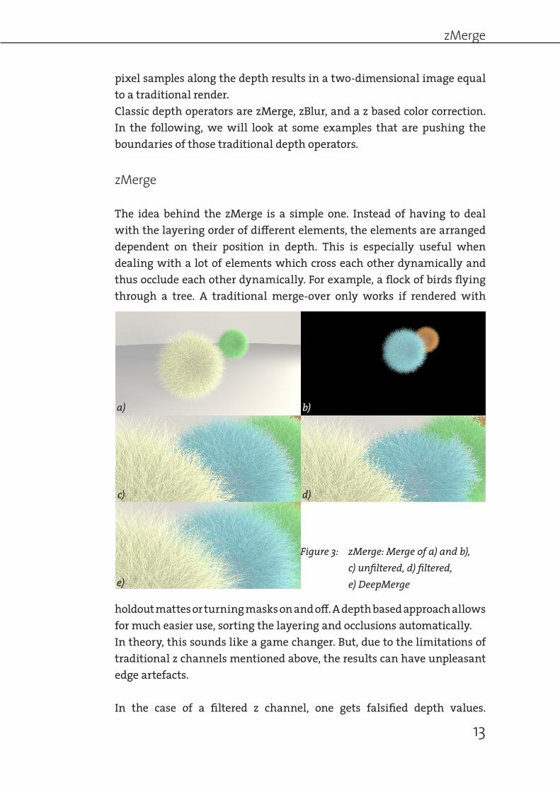
pixel samples along the depth results in a two-dimensional image equal to a traditional render. Classic depth operators are zMerge, zBlur, and a z based color correction. In the following, we will look at some examples that are pushing the boundaries of those traditional depth operators.

zMerge

The idea behind the zMerge is a simple one. Instead of having to deal with the layering order of different elements, the elements are arranged dependent on their position in depth. This is especially useful when dealing with a lot of elements which cross each other dynamically and thus occlude each other dynamically. For example, a flock of birds flying through a tree. A traditional merge-over only works if rendered with

holdout mattes or turning masks on and off. A depth based approach allows for much easier use, sorting the layering and occlusions automatically.In theory, this sounds like a game changer. But, due to the limitations of traditional z channels mentioned above, the results can have unpleasant edge artefacts.

In the case of a filtered z channel, one gets falsified depth values.

Figure 3: zMerge: Merge of a) and b), c) unfiltered, d) filtered, e) DeepMerge

a) b)

c) d)

e)


14

Consequently, semitransparent parts of the image suddenly disappear behind something else, as the depth value is inferior to the background. Using the unfiltered depth channel resolves that problem. But fine detail such as the fur in Figure 3 gets rough, as the unfiltered z channel is not accurate enough.

Zblur

To mimic the look of a real life camera, a vital element is depth of field. Depth of field can be rendered physically correct in the rendering engine, producing very good results. However, adding depth of field usually greatly increases render times. To avoid this, and to gain more flexibility over the look, depth of field is often achieved in compositing, using the z channel to drive a convolution mimicking depth of field. This produces fairly good results; but again, we will get incorrect results in semitransparent highly detailed areas, leading to glowing edges. With the use of deep compositing and the right tools, the depth differentiated opacity information can be used to produce accurate and artefact-free depth of field in compositing. Figure 4 shows the differences for similar depth of field using Nuke‘s built in

Figure 4: a) zBlur b) Frischluft c) Bokeh

a)

b)

c)

Preserving color values/corresponding to zCrop/zSlice

15

zBlur, Frischluft Lenscare (that is often mentioned as the solution to edge artefacts) and Peregrine Bokeh (being the only one that uses deep data). It is clearly visible that only Peregrine Bokeh is preserving the detail in the fur. The other tools, relying only on the zDepth channel, produce glowing with an anti-aliased zDepth channel or chunky edges without anti-aliasing. This contamination of depth information is also true for motion blur. Theoretically, deep images also allow for both depth of field and motion blur produced in compositing as the convolution happens depth independent and therefore preserves accurate depth information. Yet the tools to do this don‘t exist for the moment. Peregrine Bokeh outputs a flat image and not deep data.

Preserving color values/corresponding to zCrop/zSlice

In a traditional image, on semitransparent pixels where two objects overlap, the two color values are added together, weighted by the transparency. Therefore, isolating one element is nearly impossible; it will always have the color values of the other object in the edge pixels. This might be acceptable in certain cases, but, with an increasing number of semi-transparent pixels, the result becomes more and more visually unpleasing. With deep images this problem does not exist as every pixel has a unique value per depth. The weighted average of the pixel only has to be calculated once the image gets flattened, that is to say, converted to a traditional two-dimensional image. Thus, one gains a high amount of flexibility, gaining the ability to cleanly isolate elements

Figure 5: a) deep rgba b) deep alpha c) zDeptha) b) c)


16

that overlap. Figure 5 shows the differences of deep rgba, deep alpha and traditional zDepth in a point representation. The motion blurred area has differentiated color values only using deep rgba. The traditional anti-aliased zDepth channel produces, as mentioned before, incorrect depth values. The differentiation of color in depth also leads to the possibility of using a multitude of object IDs in a single channel. I will get back again to

this later in chapter 7.This is, of course, not true for refractions, as the refracting material will get the color of what gets refracted, and has in itself no real color.(Figure 6)

Volumetrics

Volumetric effects is where deep compositing comes in really handy.Combining volumetrics with other elements in a traditional workflow would require having the volumetrics rendered with the other objects with a black material applied. The result is a volume with holes in it where the elements are in front of it. The problem with rendering holdout mattes is, that every change in animation or staging of the elements means having to re-render the volumetric element as well. As rendering time is critical, avoiding this improves turnaround and and the time needed for changes a lot.With deep compositing one has rgba values for each pixel at each depth step. Therefore, a volumetric is fully described in a deep image. The complete holdout process can then be outsourced to compositing where a simple DeepMerge checks which sample is in front of which. The flexibility permits tweaking positions in compositing and dropping in new, or deleting unnecessary, elements as desired.This is true for live action plate elements as well. Those can be converted to a deep image, naturally only having a single depth sample, as there

Figure 6: A refracting object with the backgrond cropped

What it can‘t do

17

is no additional information. This can then either be merged or used to generate a holdout. Another advantage is the capability to combine the output of two separate render engines. When rendering the volumetric effect with one renderer and rendering the object placed in the volume in another renderer, the holdout matte would not match 100%. This is caused by the different filter kernels used in the different render engines. As the holdout mattes can be generated in compositing with deep images, this problem is solved.

What it can‘t do

The above is, however, not possible in every situation. It does not apply to any interactional changes. If the element affects the volume‘s simulation,

then this, of course, has to be resimulated and re-rendered. The same applies to light ing changes which normally require a re-r e n d e r i n g .

Nevertheless, there are possibilities to avoid re-rendering everything because of a lighting change. I will cover this as well as other interesting possibilities that deep images bring for volumetric handling in chapter 7.

Figure 8: removing the object in a) reveals a hole(b)

Figure 7: Teapots(a) get merged with fog (c) traditional holdout(b), d) and e) show the possibility to rearrange in compositing

a) b) c)

e)

a) b)


18

The structure of multiple samples per pixel might create the impression that one could simply delete a foreground object revealing what is behind. This is wrong. As the sampling stops at an opaque surface, removing a foreground object will only reveal a hole in the background wherever the foreground object was opaque (see Figure 8). Yet, this is theoretically possible and will be further examined in chapter 7 in combination with

the afore mentioned possibilities of a deep image based motion blur.Another problematic situation that deep images can not resolve is intersecting objects. Even though the depth of the different pixels is known and will be interleaved correctly, the edge will be hard and not anti-aliased. The pixel samples inside an object will most likely have an alpha value of 1 and consequently won‘t produce any blended edge.At the moment, another constraint for the use of deep images exists. World space masking or cropping, as used with a world position pass, is not yet possible. The world position pass basically saves world coordinates x y z in the three color channels r g b. With that it allows masking certain parts of an image by selecting specific colors, hence areas, in 3D space. As the masks are expressed in world coordinates, they are consistent throughout different camera angles. I will get back to this in chapter 7 as

well, pointing to solutions and further applications.

Figure 10: A world position pass(left) and a matte created from it (right)

Figure 9: merging the cubes left and right produces a rough edge (middle)

Autodesk 3ds Max and Chaos Group‘s VRay

19

3 Implementation

Being such a new Technology, deep data is not yet broadly supported by software packages. As deep images are derived from Pixar‘s Deep Shadow Maps, Renderman was one of the first renderers being able to write deep images in the dtex format. Houdini, with its Mantra renderer, is also capable of rendering deep images in its rat format. Chaos Group‘s VRay has announced deep image support in the next release. The functions are already implemented and are being deployed privately through nightly builds. On the compositing side, The Foundry‘s Nuke is the sole solution supporting deep images at the moment.The biggest issue for a long time has been a common file format. Nuke was only supporting the dtex format prior to version 7. Now, the already broadly used Open EXR file format has been extended to support deep images. Even though it is not yet released and is still in beta, it is already supported by Nuke. With this standard set, software vendors will hopefully soon converge to this new file format and deep image support will come to more and more products, therefore gaining broad awareness and application, leading to an improvement of the tool-set and implementation.In the following I am going to concentrate on Nuke on the compositing side and on Chaos Group‘s VRay for 3ds Max. Nuke is certainly the standard compositing package at the moment and the first and only one supporting deep image data. VRay is a very advanced renderer which is used more and more across the industry. This combination of VRay and Nuke is definitely a powerful one, gaining even more flexibility through the use of deep images.

Autodesk 3ds Max and Chaos Group‘s VRay

At the moment, deep compositing is not yet officially supported. However, it can be used with the latest nightly build in combination with the VRay Stereoscopic helper plugin. VRay already used “shademaps” that saved precalculated images with multiple samples per pixel. This was then used to speed up the calculation of otherwise computationally intense operations such as motion blur, depth of field as well as for rendering the second view in a stereoscopic project. The stereoscopic helper has since been extended to save deep pixel shademaps that correspond to a deep image. VRay‘s deep shademaps

Implementation

20

are saved in the proprietary VRay Shademap format *.vrst but can also be rendered as deep Open EXR 2.0. Additionally, a deep-vrst-reader plugin for Nuke and a vrst to Open EXR 2.0 command line converter are provided. VRay Shademaps are using a zlib compression, there is no plan to implement other compression algorithms. The compression is applied per render bucket. This is unavoidable as the file needs to be written bucket by bucket. Otherwise, huge files would need to be cached in ram during rendering of the whole frame. Avoiding that brings down the memory usage during rendering tremendously.Deep images are rendered with linear gamma only, there is also no other possibility for further settings.VRay does support render elements for deep images. This opens up completely new possibilities for look development and, with optional deep utility render passes, even more possibilities for post rendering tweaks and effects without the negative side effects and artefacts mentionend in Chapter 2.At the moment, volumetric renderings are

only supported for Chaos Group‘s own fluid dynamics tool-set Phoenix FD. This is due to the necessity of a geometry shader in order to render deep shademaps. To render Phoenix fluids to a deep image file in VRay one has to enable the geometry mode for the fluid simulation under the rendering tab. Naturally, one will also need to check the maximal transparency levels in the rendering->Global switches tab. This delimits the maximum amount of samples a ray traverses before the calculation stops. Setting these too low will result in not getting to the volume itself in the worst case. A rough approximation can be done by dividing the box size by the cell size.Other factors influencing the amount of depth samples and the way they are sampled, are the step size and the cell and box size. The step size can be seen as a sample rate for the fluid rendering. With a higher value, the samples are further apart, therefore resulting in fewer samples. This will

Figure 11: settings for the stereoscopic helper

The Foundry‘s Nuke

21

not only influence the amount of deep samples generated but also the way the fluid is sampled. And, consequently, the quality of the fluid rendering decreases with increasing step size. Unfortunately, the current version 2.0 of Phoenix FD has a bug. It causes the resulting deep images to have black rgba samples throughout the whole fluid container and not just for the actual fluid itself. This greatly increases the number of samples and is clearly reflected in a higher file size. This will most likely be fixed in the next version, though.


Nuke has been supporting deep images since version 6.3, having implemented WETA Digital‘s tool-set. Prior to version 7, the only supported file format was Renderman‘s dtex file format. Nuke has different operator types, image operators(IOps), geometry operators(GeoOps), particle operators, and deep operators(DeepOp)9. This is important to understand, since due to the three-dimensional nature of the deep image files, there are two independent worlds inside Nuke. One is the dedicated deep operators which handle similar operations as the classical two-dimensional image operators. These have to be used and can not be substituted by their two-dimensional relatives. Still, there‘s a way of exchanging data from one world to another. The DeepToImage node basically flattens the deep image to a two-dimensional image with only one single value per pixel. All premultiplied samples along the depth of a pixel are accumulated to a single value, resulting in a traditionally known image. The option “volumetric composition” defines whether the deep.back values get used for the merging process or not.In contrast, DeepFromImage takes a two-dimensional image and converts it to a deep image, naturally only with a single depth sample. Depth is extracted either from an existing zDepth channel or from a uniformly specified depth. Very similar is DeepFromFrames, the difference being that it samples the input at multiple frames and places them at various depths, building a volume. Each frame can be seen as a depth slice. The maximum and the minimal depth can be set and sample frames are placed in between those boundaries. With the combination of animated noise and DeepFromFrames, one can easily build a varying volume fog. There is a fourth node that connects an IOp with DeepOps: the DeepRecolor

9 c.f Harvey, V., Brady, A., Ring, D., Binks, J., Wadelton, J., Hughes, M. 2013.

Implementation

22

node. It uses a flat image‘s color values and takes only the depth values from an existing deep image. The resulting deep image will have several depth samples if the deep image that was input has multiple depth samples. However, the color values will be the same at every depth, i.e., an averaged color of the overlapping objects. This makes sense, as they originate from a two-dimensional image. The result can be seen as a deep alpha instead of a deep rgba image. I would therefore discourage using the DeepRecolor to simply transform flat images to deep images, as it constitutes less information than a full deep image rendering and doesn‘t tap the full potential of a deep image compositing workflow. The great advantage of deep compositing is actually the clear separation of values from different objects and thus depths.Operators which only take a deep input and return a deep image as the result are called DeepOnly operators.Most of the DeepOnly operators are very much a deep implementation of their two-dimensional relatives, making use of the additional depth information. To begin with, there is DeepReformat that acts exactly like its two-dimensional counterpart and reformats an image to a new format, scale or box with the possibility of resizing it. DeepCrop allows cropping a deep image not only to a certain region in x and y but allows cropping it in depth as well. Additionally, it gives the option to crop either the inside or the outside of the defined region.DeepTransform is a very simple implementation of its two-dimensional relative, allowing for translation in x,y and z only, as well as scale in z. This is understandable as any operation that would break the structure of the three-dimensional raster, e.g. rotation, would result in need for interpolation. Consequently, the information would be falsified. Since most of these transforms don‘t need the additional depth information, they can easily be applied once the deep image is transferred back to a flat

Figure 12: Point representation of a cube(left) and the same with DeepTransform with noise as mask applied(right)


23

image. DeepTransform also offers the possibility of using a mask on the z based operations. This can be very useful, as it allows to quickly push back or pull out specific areas which should rather be in front of/behind a particular object. Furthermore, using a noise can provide additional irregularity (c.f. Figure 12).Another tool in Nuke‘s deep compositing tool set is DeepColorCorrect. Like its two-dimensional counterpart, it allows for all the known color correction parameters – including separate correction of highlights,

shadows and mid tones. Using the zmap knob in the Masking tab, the color correction can be limited to a specific depth. Moreover as deep images save one sample for every depth per pixel the color correction is differentiated in depth. It opens the possibility to treat every single pixel and every single depth on its own. As color correction is one of the basic operations in compositing, this is a vital operator that can be used for different purposes when dealing with channels other than rgb. Unfortunately, the DeepColorCorrect doesn‘t have a mask input.The DeepExpression node is very powerful, as it allows manipulating the image using expressions. Unfortunately, it doesn‘t use the exact same syntax as the 2D Expression node and lacks many of the mathematical expressions known from its 2D counterpart. I‘ll get back to this later in this chapter.Apart from manipulating images, compositors also need to combine

Figure 13: Result of a DeepColorCorrect restricted to a specific depth slice

Implementation

24

different images. The same is true for deep images, of course. Nuke offers two different options. The first is DeepMerge. It has two different modes. In “combine“ mode, the different depth samples are interleaved according to their particular depth value. If two depth samples have the same depth, they are both written to the resulting deep image. The order in which they are interleaved is then deducted by the input order on the node with B being the first input. Enabling “drop hidden samples” will delete samples that are behind a fully opaque sample. This can be useful to reduce the data that has to be processed further down the tree.The “holdout“ mode produces a held out deep image. The way it works is to subtract the alpha of input A from the alpha of input B. Samples that have an alpha inferior or equal to 0 are deleted and the color channels premultiplied with the resulting alpha values.The holdout operation also exists as individual node. The difference to the DeepMerge is that it outputs a flat image instead of a deep image.

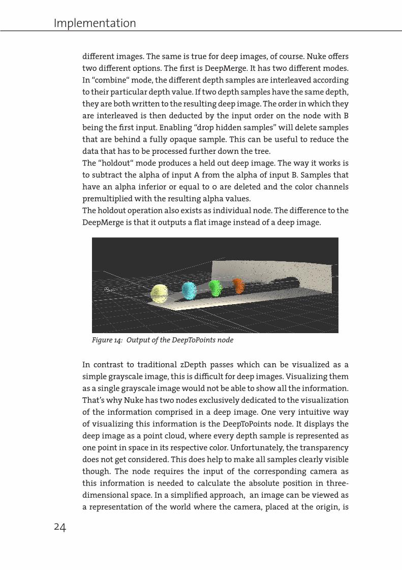
In contrast to traditional zDepth passes which can be visualized as a simple grayscale image, this is difficult for deep images. Visualizing them as a single grayscale image would not be able to show all the information. That’s why Nuke has two nodes exclusively dedicated to the visualization of the information comprised in a deep image. One very intuitive way of visualizing this information is the DeepToPoints node. It displays the deep image as a point cloud, where every depth sample is represented as one point in space in its respective color. Unfortunately, the transparency does not get considered. This does help to make all samples clearly visible though. The node requires the input of the corresponding camera as this information is needed to calculate the absolute position in three-dimensional space. In a simplified approach, an image can be viewed as a representation of the world where the camera, placed at the origin, is

Figure 14: Output of the DeepToPoints node


25

not moving; instead, the content is moving. This representation needs to be translated back to world-space where the objects stand still and the camera is moving.The mathematical relationship between a three-dimensional object and its mapping onto an image plane can be described with the model of an ideal pinhole camera. The ideal pinhole camera is the most basic representation of a photographic image. Although the image is affected by the different optical lens elements in the real world, this is most of the time neglected in computer graphics, as those effects are either very small or can be recreated afterwards. The model of the pinhole camera is based on the perspective projection which maps object points in three-dimensional space onto a two-dimensional plane. The light ray travels from the object point to the projection center. The mapping onto the image plane takes place at the point of intersection between this ray and the image plane. In photography the image plane, this being the film or the sensor, lies behind the projection center, which is the focal point of the lens. Therefore, the rays are extended and the resulting image is

z

xx‘

d

aperture

FOVfocal

Figure 15: Relations between points in 3D space and their projection onto a 2D plane

Implementation

26

upside down. For camera simulation in computer graphics, this can be simplified by placing the image plane in front of the projection center. The camera model is described by three intrinsic parameters and six extrinsic parameters, defining its location and orientation in 3D space. The six extrinsic parameters defining the camera’s location in space are the three translations in x,y and z and the three rotations around x,y and z. The intrinsic parameters are the field of view (fov) and the dimensions of the image plane in x and y as well as, if the depth information needs to be preserved, the near and far clipping planes. With these parameters, a camera projection matrix can be built10.

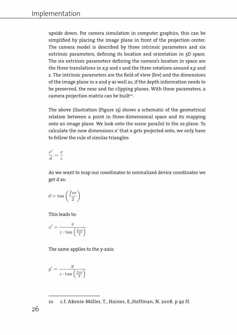
The above illustration (Figure 15) shows a schematic of the geometrical relation between a point in three-dimensional space and its mapping onto an image plane. We look onto the scene parallel to the xz-plane. To calculate the new dimensions x‘ that x gets projected onto, we only have to follow the rule of similar triangles:

x0

d=

x

z

As we want to map our coordinates to normalized device coordinates we get d as:

d = tan

✓fov

2

◆

This leads to:

x0 =x

z · tan⇣

fov

2

⌘

The same applies to the y-axis:

y0 =y

z · tan⇣

fov

2

⌘

10 c.f. Akenie-Möller, T., Haines, E.,Hoffman, N. 2008. p 92 ff.


27

With this, the projection is defined. However, one wants to express this as a matrix. To express any transformation in computer graphics, homogeneous coordinates are used. This essentially adds a fourth row to the matrix to allow for scaling and translation with a single matrix. Instead of having just x,y and z one gets x,y,z and w. To transform homogeneous coordinates back to cartesian coordinates, x,y and z have to be divided by w. For projection, this is very convenient as we need to divide everything by z. As everything gets divided by w, one has only to make sure that the value of z ends up in w. The projection matrix will therefore be:

2

6664

1

tan( fov2 )

0 0 0

0 1

tan( fov2 )

0 0

0 0 0 00 0 1 0

3

7775

Yet, we loose our z information. Therefore, we need to find a way of including the normalized z value as well. We know that the far clipping plane should be mapped to -1 and the near clipping plane to +1.

z0 = a · z + b

with 1 = a · zFar + b and 1 = a · zNear + b

Our final term is:

z0 =zFar + zNear

zFar zNear· 2 · zNear · zFar

zNear zFar

Combining this leads to the following projection matrix:

2

6664

1

tan( fov2 )

0 0 0

0 1

tan( fov2 )

0 0

0 0 zFar+zNear

zFarzNear

2 · zNear·zFar

zNearzFar

0 0 1 0

3

7775

Implementation

28

This gives the normalized camera coordinates and assumes that the camera is located in the origin. To get screen space coordinates of a camera anywhere in space, what we need, is to consider the camera transformation (derived by the extrinsic parameters), to scale the coordinates to pixel coordinates and to account for the aspect ratio. This can be expressed as a series of matrix multiplications.

The second node to visualize deep data is the DeepSample node which shows a list of all depth samples of a chosen pixel and their values in a list view. This allows one to get the exact values and see what exactly is going on numerically. In addition, it shows the minimal and maximal z value as well as the sample depth (amount of samples) for that pixel. It is a very valuable node for trouble shooting as the values can be compared and the operations reproduced.Another useful tool that, unfortunately, isn‘t part of the Nuke tool-set is DeepSampleCount. However, the source code is available in The Foundry‘s NDK Dev Guide. It writes the sample depth per pixel into a traditional image which makes it easy to see the repartition of sample depth over the whole image.It is also possible to pick pixel values in the viewer. The corresponding depth values are shown in the depth graph in the viewer window. The depth graph shows the alpha value as a function of depth. This is a good way to quickly get an image of the depth development (Figure 17).

Figure 16: Control panel of the DeepSample node


29

Figure 17: Depth graph with a single pixel sampled (top) and a region sampled (bottom)

As of today, there are still a lot of issues with Nuke‘s deep compositing tool set. A full list of filed bugs and their corresponding IDs can be found in the appendix.One field that is missing a lot of functionality is the way to interact with deep compositing nodes via Python. The functions node.width() and node.height() return the root format rather than the format of the actual image stream. This poses rather big problems when trying to extend the functionality of the tool-set, as the format is always needed when trying to sample over an image. Information on width and height is also necessary to deduct screen space relations. Another function that is vital to integrate a custom extension of the tool-set is node.channels() which returns an empty list for deep images.Furthermore, the file handling of deep image files is not yet completely thought-out. Open EXR 2.0 is only supported for deep images and not for traditional images. In addition, Nuke does not recognize whether an EXR file is a deep image or not – thus one has to choose files through the specific node instead of drag-and-dropping or using keyboard shortcuts. One solution to avoid this issue is using a separate file extension(.odz) as proposed in „Technical Introduction to Open EXR“11. When comparing the deep read node to the traditional read node, the lack of a colorspace knob is apparent. Even if it is recommended to always render an image with a linear gamma, which also holds true for deep images, there are still cases where the image has another gamma and needs to be transferred to a linear gamma in order to work inside Nuke. The lack of several color related functions raises the question whether colored deep images are used in production at all right now.A big issue for building custom tools is the lacking functionality of the DeepExpression node. A lot of the functions available in the traditional


Implementation

30

expression node do not work in the DeepExpression node. Further, more complex expressions are not evaluated correctly. It should also incorporate depth specific functions as sampleDepth, zmin and zmax. This restricts the use of this otherwise very useful node considerably.Another problem is posed by the not fully supported bounding box. This leads to distorted point clouds, when using DeepToPoints. DeepToPoints uses the bounding box as format and not the format itself which leads to a totally wrong representation of the points in three-dimensional space. To avoid this, a crop node can be used, resetting the bounding box to the

whole image.

Figure 18: The distorted result of DeepToPoints (left) and the correct result (right)

31

4 Performance

A new technique might bring big advantages, but is it reliable enough for production use and does it work in a day-to-day routine? One of the key factors in answering these questions is the infrastructure. Is it ready for the new technique or does it need to be adapted to accommodate a flawless use of such a game changer.Image processing is still one of the most computationally intense operations. Hence, visual effects facilities are remarkably always employing state of the art technology and hardware in order to build a high performance infrastructure, able to handle big amounts of image data in the shortest processing times possible. On the other hand, they are trying to achieve this goal with a minimal budget to stay competitive.Still, the resource hungry simulations, renderings and compositing operations always push the existing infrastructures to their limits in the quest of producing steadily increasingly astonishing pictures.A new technology can only be employed if the infrastructure allows for a fluent way to use it. This is also true for my goal of judging the production readiness of deep compositing.

There are different hardware components that are being used to deal with image data in a visual effects infrastructure. Most important are the processors themselves which have to deal with most of the calculations for each pixel and the memory, as a fast storage for image data, which enables, for example, real time playback or caching of data that is continuously written to disk. As visual effects depend heavily on collaborative work, most of the data is stored on a central server and has to be moved from and to the server from the workstations12. Furthermore, hard disks, as storage for all the data, are a very important factor as well. Graphics cards become more and more important for real time visualization and for heavily parallelized computations. However, as they are not yet commonly used for rendering or compositing purposes, I will not count them as core important hardware components.

12 c.f. Novy, D. in Okun & Zwerman. 2010. p. 807

Performance

32

This leads to the following important performance indicators for a deep compositing workflow:

•file size•processor usage•memory usage•network load

File size

As deep images save multiple samples per pixel, one performance issue is clearly deductible. Saving more information is directly connected to bigger file sizes. Without compression, the relation between sample count and file size is proportional. The chart (Figure 19) shows the relationship between sample count and file size. The data was taken from a volumetric rendering sampled with different step sizes and therefore the content is approximately the same. The relation is linear. So, in general, using deep compositing will increase file sizes. However, file size is directly proportional to the sample count.

As different applications need a different amount of depth samples, the performance of deep images is highly dependent on the use case and the content of the image. A great differentiation can be made between hard surface renderings compared to volumetric renderings.To correctly judge the increase in file size, a look at the information stored in the file is needed. I will consider an Open EXR 2.0 image, as this is most likely to become the standard format for deep images. The comparison is

0 1000 2000 3000 4000 50000

200

400

600

800

1000

1200

file size in MB

samples

Figure 19: Relation of sample count and uncompressed filesize

File size

33

16bit

16bit

16bit

16bit

32bit

32bit

32bit

red

green

blue

alpha

deep.front

deep.back

depth samples

Figure 20: Bit depth of the elements that make up an OpenEXR 2.0 deep image

based on commonly used 16 bit half float EXR files, which contain every channel with 16 bit floating point precision. Most commonly, an image contains 4 components (r, g, b and a), resulting in the use of 4 * 16 bit = 64 bit per pixel. As compression is heavily dependent on the image content and its redundancy, (which I‘ll discuss later) it is not taken into account for these calculations, to allow for unbiased results.With no additional information – in other words: with a single sample per pixel – a deep image will have an increased file size of 96 bit per pixel compared to a traditional image. This is 32 bit each for deep.front, deep.back as well as the sample count13. With every additional depth sample the file size increases by another 128bit, 64 for rgba and 64 for deep. This means that a 16 bit deep EXR file will have double the size of an rgba 16 bit EXR. This seems drastic but is comparable to an additional layer in a multilayer EXR file. A further increase of the file size is then directly proportional to the sample count. Figure 22 shows the different parts that make up the file size for deep images compared to traditional flat images.Looking at different image content means that for hard surface renderings file sizes stay relatively low, as additional samples are only introduced through semitransparent pixels. This will, in most of the cases, be edge pixels which are semitransparent due to anti-aliasing or motion blur. As it is fairly unlikely that a lot of objects share the same edge pixels, the amount of additional depth samples stays relatively low as well. Figure 21 (a) shows a fur rendering. This is one use case that has a lot of detail and, therefore, a lot of anti-aliased semitransparent pixels and thus, a relatively high sample count. Hair and fur might be the application that will result in the highest sample count apart from volumetrics. Figure 21 (b) shows all pixels which have an alpha<1, and so have additional depth samples. This is approximately 15% of the image. The maximum sample depth is 4. Figure 21 (c) shows the amount of depth samples per pixel, with 1 for the

13 Thanks to Peter Pearson and Jonathan Egstad for the hint!

Performance

34

lowest level and 4 for the highest level. In total, this makes it roughly a seventh (~15%) more samples in total as opposed to its flat relative. Figure 20 shows the different elements that contribute to the file size. Though the increase of file size is clear and apparent, it is not alarming for non volumetric files.In contrast, volumetric renderings result in much bigger file sizes, depending solely on the sample rate. As the sample rate is an arbitrary parameter, file sizes can range from approximately the same size as its two-dimensional sibling up to theoretically infinite size. Hence it is very important to choose the sample rate wisely. A low sample rate will potentially not provide enough detail for the given application yet a high sample rate will result in large files that might be hard or impossible to process. In this context, it becomes clear that alternative sampling models (e.g. proxies) are needed to improve the work with large volumetric files. These will be discussed in Chapter 6. For additional layers, for example render elements and utility passes, the increase in file size is related to the amount of channels saved. In uncompressed files, the increase in file size can be expressed as the product of the sample count and 16 (respectively 32) bit for any additional channel. Since deep images come at the cost of an additional 64 bits per sample and an additional 32 bits per pixel, saving multilayer deep EXR files for additional channels instead of single files should be considered, as single files always have to save the additional depth information but deep multilayer exrs save it only once (c.f Figure 22).

Figure 21: a) Fur rendering, b) pixels with more than one sample, c) sample count represented as the height of layers

b)

c)

a)

Processor and memory usage

35


Deep images are generated in 3D rendering and used in compositing. Hence, these two areas’ performance needs to be evaluated in order to draw a conclusion about the influence on performance from deep image data on common IT infrastructure.The way a 3D rendering uses the hardware differs slightly from the way hardware is used in compositing. Usually, render times for 3D renderings are much higher than 2D render times. The usual performance footprint of a 3D rendering is a 100% processor usage for the time a bucket is calculated. During that time memory usage increases, as the bucket is written to memory and then written to disk or a network storage. Thus, the network load is most of the time very low, only becoming a little higher once a bucket or frame is written to disk. The bottle neck is clearly the CPU for 3D rendering. However, depending on the complexity of the scene and texture maps, memory can increase as well, as all this needs to be loaded into memory before rendering.In compositing, network and memory are much more important, as the ultimate aim is to have a (close to) real time feedback. Thus, image data has to be accessed at a very high frequency and caching it to disk or memory helps a lot to speed this up. As mentioned before, deep images produce larger files based on their nature of saving multiple samples per pixel. This is also the primary reason for decreased performance, influencing especially memory and

0

50000000

100000000

150000000

200000000

250000000

300000000

350000000

400000000sample count

deep.back

deep.front

a

b

g

rdeepdeep from flatflatflat

bits

Figure 22: Total bits per file and the corresponding repartion of the channels

Performance

36

network usage.

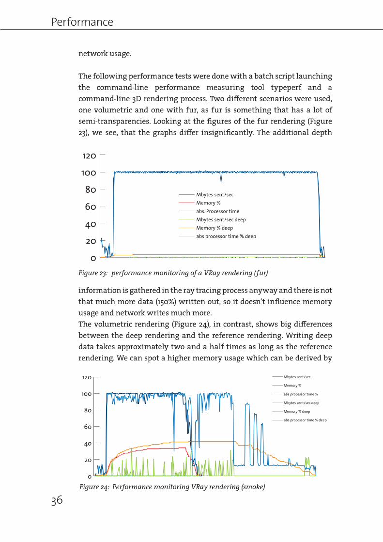
The following performance tests were done with a batch script launching the command-line performance measuring tool typeperf and a command-line 3D rendering process. Two different scenarios were used, one volumetric and one with fur, as fur is something that has a lot of semi-transparencies. Looking at the figures of the fur rendering (Figure 23), we see, that the graphs differ insignificantly. The additional depth

information is gathered in the ray tracing process anyway and there is not that much more data (150%) written out, so it doesn‘t influence memory usage and network writes much more.The volumetric rendering (Figure 24), in contrast, shows big differences between the deep rendering and the reference rendering. Writing deep data takes approximately two and a half times as long as the reference rendering. We can spot a higher memory usage which can be derived by

0

20

40

60

80

100

120 Mbytes sent/sec

Memory %

abs processor time %

Mbytes sent/sec deep

Memory % deep

abs processor time % deep

Figure 24: Performance monitoring VRay rendering (smoke)

0

20

40

60

80

100

120

Mbytes sent/secMemory %abs. Processor timeMbytes sent/sec deepMemory % deepabs processor time % deep

Figure 23: performance monitoring of a VRay rendering (fur)


37

the buffered image and, respectively, the single buckets held available in memory. In addition, the amount of data that has to be sent through the network interface to a central server is a lot higher than with a traditional image rendering. Nevertheless, it still doesn‘t reach critical amounts in this test and stays under the practical throughput of 100 Megabytes per second of a standard Gigabit interface. This is most likely the minimum connection type adopted by most of the industry14. Still, this increased network traffic needs to be considered when looking at distributed rendering with a render farm, as most facilities are using. In that case, the network load will add up with every rendering node posing a heavy load on the server.

Looking at performance influences on compositing with deep images (Figure 25), we see that the difference is already much more apparent. In this case, a deep image was rendered as normal 2D EXR. In comparison to the processing of a normal image, the processor usage is much higher with deep images. This is due to the elevated amount of data that has to be processed. Additionally, a conversion from a deep image to a traditional image is done and involves resampling and thus needs processing power. Whereas for a normal image, the whole processing power isn‘t even needed. Also, memory usage is drastically elevated, as the image gets loaded into RAM. The most striking parameter, however, is network usage. It tops out around 110 Mbytes and only falls during the processing time. This processing can be attributed to the conversion into a flat image.A deep image is first loaded into memory when it needs to be processed. Its size in memory corresponds approximately to the uncompressed file size. If the files are too large, they are not cached, but only read sequentially. In

14 c.f. Novy, D. in Okun & Zwerman. 2010. p. 808

0

20

40

60

80

100

120Mbytes received /sec flat

Memory % flat

Abs Processor Time % flat

Mbytes received /sec

Memory %

Abs Processor Time %

flat

Figure 25: Performance of a Nuke rendering

Performance

38

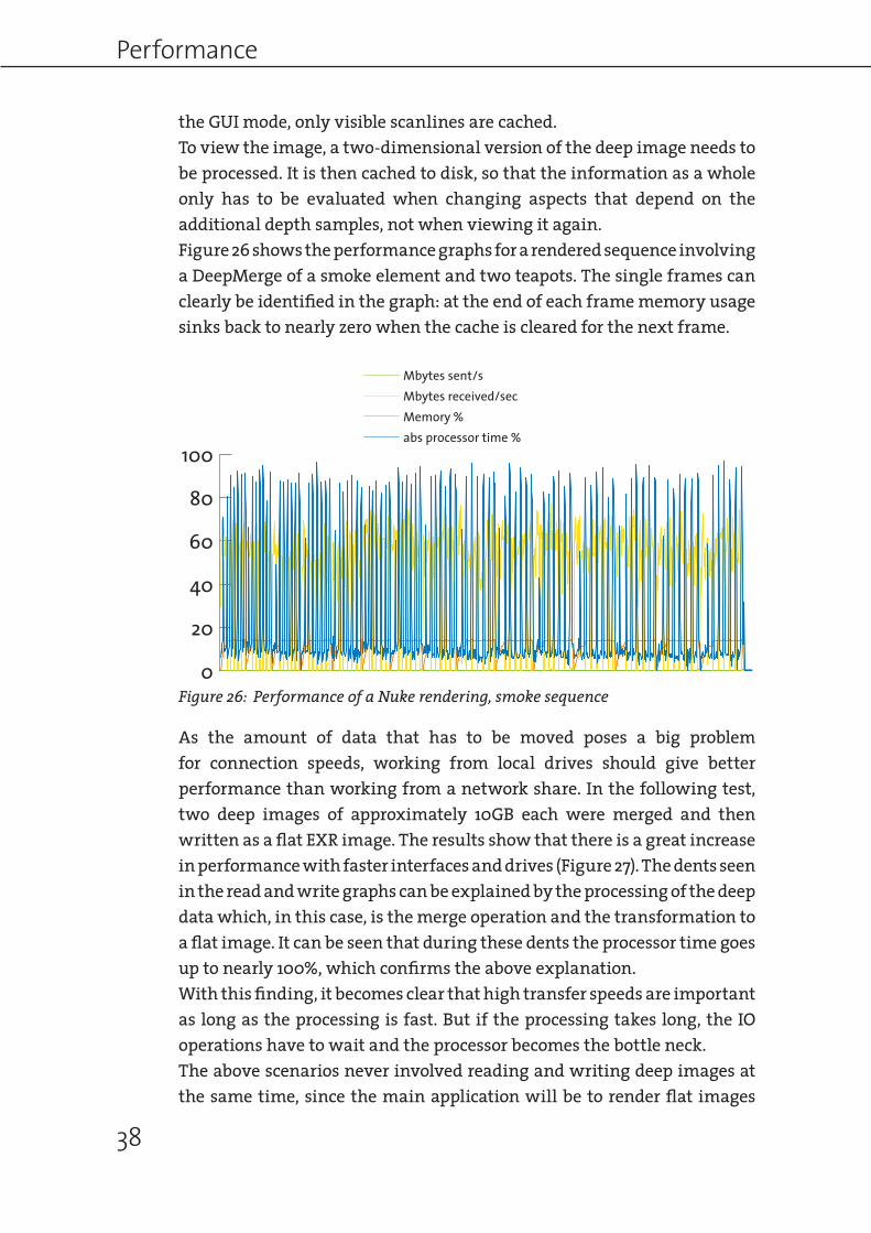
the GUI mode, only visible scanlines are cached.To view the image, a two-dimensional version of the deep image needs to be processed. It is then cached to disk, so that the information as a whole only has to be evaluated when changing aspects that depend on the additional depth samples, not when viewing it again. Figure 26 shows the performance graphs for a rendered sequence involving a DeepMerge of a smoke element and two teapots. The single frames can clearly be identified in the graph: at the end of each frame memory usage sinks back to nearly zero when the cache is cleared for the next frame.

As the amount of data that has to be moved poses a big problem for connection speeds, working from local drives should give better performance than working from a network share. In the following test, two deep images of approximately 10GB each were merged and then written as a flat EXR image. The results show that there is a great increase in performance with faster interfaces and drives (Figure 27). The dents seen in the read and write graphs can be explained by the processing of the deep data which, in this case, is the merge operation and the transformation to a flat image. It can be seen that during these dents the processor time goes up to nearly 100%, which confirms the above explanation. With this finding, it becomes clear that high transfer speeds are important as long as the processing is fast. But if the processing takes long, the IO operations have to wait and the processor becomes the bottle neck.The above scenarios never involved reading and writing deep images at the same time, since the main application will be to render flat images

0

20

40

60

80

100

Mbytes sent/sMbytes received/secMemory %abs processor time %

Figure 26: Performance of a Nuke rendering, smoke sequence


39

from deep images. A conversion from one deep file format to another would involve a simultaneous read and write process of deep data. Figure 28 shows the test results of Nuke converting a vrst file to an Open EXR 2.0 file. The write operations are much slower than the read

0

20

40

60

80

100

0

20

40

60

80

100

120

0

50

100

150

200

250Write Mbytes/secRead Mbytes/secMemory %abs processor time %

Read from server

Read from local HDD

Read from local SSD

Figure 27: Performance comparison of server, local HDD and local SSD

Performance

40

operations. Additionally, as the data doesn‘t have to get sampled, the processor usage is lower.The impact of deep images on compositing are apparent. Due to the elevated amount of data that needs to be loaded, cached and processed, processing times rise and make a real-time feedback nearly impossible. To allow for a smooth work concepts like proxies or regions of interest should be considered. These are further discussed in chapter 6.

Network

As previously mentioned, visual effects facilities usually distribute the rendering onto a multitude of machines - a render farm. The source and output data is stored on a central server. As several render nodes read and write to and from this server at the same time, it is a crucial factor for the performance of the infrastructure. With the increased file sizes of deep images, this becomes even more important. The following performance test is exemplary and is meant to show problem areas and limitations of deep image rendering. As the performance of a network depends on a multitude of different factors, the goal of this test is not to find an ultimate solution for the handling of huge deep data renderings but rather to illustrate problem areas and identify behaviors and patterns of such a rendering process. In the following performance test, the network load on the server is tested for a VRay rendering. The rendering consisted of 50 frames of CG fog. The resolution was 2048x1556 pixels with a maximal sample depth of 800 samples per pixel. The resulting files have a size of approximately 10 GB per frame. The reference rendering on a single machine (with otherwise un-used network) took 7:51 minutes. The test

0

20

40

60

80

100

120Mbytes sent/secMbytes received/sMemory %abs processor time %

Figure 28: Performance of a Nuke rendering, reading and writing a deep file

Network

41

0

100000000

200000000

300000000

400000000

500000000write bytes/sec

Figure 29: Network trafic (write bytes) of the server

0

20

40

60

80

100

120

0

20

40

60

80

100

120

Mbytes sent/secMemory %abs Processor time %

Figure 30: Examplary performance of a render node (top) and reference of the same (bottom)

Performance

42

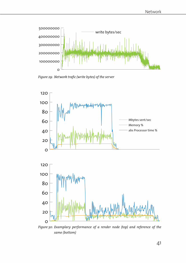
setup used a total of 16 render nodes, which would translate to a small studio‘s setup. The server‘s network interface traffic was monitored with munin15 and a custom script which recorded the output. Typeperf was used to monitor every render node with the same setup as previously used for the standalone tests. Looking at the server‘s incoming network traffic (Figure 29), a short first peak around 435 MB/sec can be observed. This quickly drops and stabilizes around 200 MB/sec. Throughout the whole rendering process, the server stayed responsive. At first look, this seems

15 c.f. munin-monitoring.org

0

100

200

300

400

500

600

0

100

200

300

400

500

600

network write Mbytes/sec

bytes sent/sec %abs Processor time %

server:

render nodes:

Figure 31: Processor time and bytes sent/sec and fall symultaneously to the write bytes on the server

Network

43

all good. However, a look at the performance figures of the individual machines reveals a great performance decline. Figure 30 shows the performance figures of the first frame on the network rendering test. What is striking is that processor usage is near 100% for the first 100 seconds and then plummets drastically to stabilize around 20-40%. At the same time, the network writes drop from approximately 20-40MB to 10-20MB. This behavior can be noticed on almost all render nodes at roughly the same time (see Figure 31). Additionally, the network traffic on the server sinks from 400 to 200MB/sec in exactly the same moment. What can be deduced here is that the server is slowed down by simultaneous writing operations of big data from multiple machines. When a certain threshold is reached the server slows down. Exceeding this threshold will cause serious loss of performance. What is strange is that the network speed influences the processor usage. This would be explicable if the image was directly written to the server. However, I assume that every bucket is buffered in memory before being written. Consequent on the decreased processor usage, the rendering takes about twice as long. This is critical and would present a substantial constraint on a real production.A similar behavior can be seen for a Nuke rendering on the farm. The render times of the individual frames go up significantly. Figure 32 shows

the traffic on the server‘s network interface. Figure 33 shows a performance comparison for one frame using a network rendering compared to a single rendering. This test used the same merge operation used in the other Nuke performance tests above and was rendered on a total of 5 render nodes simultaneously. Even though the maximal bandwidth is not reached, the

0

100000000

200000000

300000000

400000000

500000000write bytes/sec

Figure 32: Write Bytes/sec on the server during a Nuke network rendering

Performance

44

render times get longer.The insight gained from this analysis shows how crucial the server is in such an infrastructure. In this case, it is the bottleneck. Before deep compositing is used in production, the network infrastructure should be analyzed thoroughly and, where necessary, be adapted to optimize the use of deep images.

0

20

40

60

80

100

Mbytes sent/sec

Mbytes received/s

Memory %

abs processor time %

0

20

40

60

80

100

120

Figure 33: Performance during an examplary frame on a network rendering(top) and single rendering (bottom)

Compression

45

Compression

To minimize the performance issues that arise when using deep data, compression is an essential topic. There are two main categories of compression, loss less and lossy compression. Loss less compression is a reduction of redundancy, where redundant information is eliminated and encoded as less data. Loss less compression permits the exact reconstruction of the original file. Lossy compression, on the other hand, reduces information which is considered irrelevant or at least less relevant. However, the original cannot be reconstructed by the decompression – only a very close approximation to the original.

Deep images introduce additional accurate information into the compositing workflow. This information has to be as accurate as possible. Lossy compression would falsify this valuable information and by that make it useless, as it would again introduce artefacts. Thus, in the following, I will give a more in-depth look at loss less compression methods only.According to Shannon, the maximal compression possible is determined by the entropy of the source. The more redundancy there is, the more it can be compressed.16

Compression for deep images is currently using the open-source zlib compression library based on the „deflate“ algorithm by Phil Katz17. It uses a combination of the LZ77 algorithm and a Huffman encoding.

The aim of the LZ77 algorithm by Lempel and Ziv is to compress repeated information. The algorithm makes use of a so called „sliding window“ which defines the length of the known previous data stream. If any character sequence is identical to the data in the sliding window it is compressed to a pointer defining how many characters after the beginning of the sliding window the identical sequence starts, and the length of the identical sequence.18 19

16 c.f Shannon, C.E. 1948. p. 1417 c.f. Kainz, F., and Bogart, R. 2011. p. 1318 c.f. Ziv, J., and Lempel, A. 1977. 19 c.f. Feldspar, A. 1997.

Performance

46

The Huffman encoding is entropy encoding similar to the Shannon-Fano algorithm20. It uses probabilities of data to weight them and to give often recurring data a shorter encoding than data that is used less often. The weights can either be defined in advance (which is a less optimal compression) or they can be calculated by processing the data prior to the actual compression process. This will, however, take more time, since the whole data has to be evaluated beforehand. Once every data sequence has a weight, a Huffman tree is constructed. In the beginning, the two entries with the lowest weights are taken to build a leaf node. Then this node is put back into the list of data sequences with the summarized weight of both children. Then this procedure is repeated until all data sequences are inserted into the tree. To deduct the code from the tree, one has only to add a 0 for the left child or a 1 for the right child node. High weighted entries will now sit near to the root, resulting in a shorter code. Not often occurring data will be encoded with a longer code, which is not a problem since it occurs very rarely.

The deflate algorithm reduces file size by reducing redundancy first with the LZ77 algorithm and then with entropy encoding the whole data stream. A photographic image usually gets compressed to 45-55% of the original image21. The more regular an image is, and therefore the higher the redundancy is, the higher the compression ratio can be. A very noisy image tends to be hard to compress with the deflate algorithm.

20 c.f. Feldspar, A. 1997. 21 c.f. Kainz, F., and Bogart, R. 2011. p. 13

A B C D E7 4 2 5 9

A D E7 5 9

E9

B4

C2

BD

9

D A

E5 7

9DA

12BDE

18root

B4

C2

BD

9

D A

E5 7

9DA

12BDE

18

B4

C2

BD

9

D A5 7

DA

12

B4

C2

BD

9

Figure 34: Building a Huffman tree

47

Compression

However, the deflate algorithm allows for a very fast decoding which is very important for compositing tasks, as they need to be the closest to real time as possible.22

The deflate algorithm in EXR can be used on tiles and on scanlines. In practice, scanlines will give faster access times for use in Nuke. This is because Nuke‘s viewer is scanline based. At a zoom ratio of 1/n only every n-th scanline is retrieved from the file and therefore, using scanlines significantly decreases access times. With a tile based compression this would not be possible, as the whole tile would have to be retrieved in order to decode the tile and with that, access the scanline.

Furthermore, as the network is the primary bottle neck for deep compositing, compression algorithms that compress more, but are slower to decode, should be considered. If the CPU has to wait for the network interface, it can process decoding in the meantime and reduce the overall data that has to be moved.One such algorithm already used in formats such as JPEG 2000 and also as part of the compression algorithms used in the Open EXR format, is the wavelet compression. As the name suggests, wavelet compression is based on a wavelet transformation that is then entropy encoded comparable to the way the afore mentioned deflate algorithm works. The wavelet transformation is an enhancement of the Fourier transformation. The basic concept behind it is the transfer of information from two-dimensional space into frequency space. The advantage is that the frequencies present in the image are much more redundant than a pixel array.

After all, it will always be a trade of file size against accessibility. The compression will also always depend on the image content and therefore on the use case. This is why the decision has to be made depending on the circumstances. For certain cases, even a lossy compression might be

acceptable.


The visual effects pipeline

48

5 The visual effects pipeline

There are different use cases and workflows in a computer graphics based media production. The first differentiation should be made between full CG animation movies and visual effects enhanced live action movies. With movies like „Avatar“, this separation can‘t always be clearly made and defined. The lines between the two fields become blurred more and more23. Still, the workflows and pipeline requirements differ. In a CG animation movie all the content is purely computer generated. Therefore, the shot count often exceeds by far even those of visual effects heavy feature films. The pictures often have a very specific look but usually don‘t need to look photo-real24. In contrast, visual effects for live action movies usually require completely photo-realistic computer generated imagery that needs to blend seamlessly with live action plates. However, those visual effects usually only make up part of the film. Therefore, the amount of shots is smaller compared to an animation film.A further differentiation for the use of deep compositing should be made for the different rendering workflows that the various studios have adopted. This usually goes hand in hand with look development. This process can either be situated more on the side of the 3D department, trying to define the look in rendering, rendering out a perfect image, or it can be achieved in compositing, by rendering a lot of additional render passes, enabling the compositing artist to tweak most parts of the image after the rendering25. The border between them is very fluent. Often, a look development artist is experienced in lighting and rendering as well as in compositing and changes aspects of both on the fly in an iterative process. The emphasis on either workflow will unquestionably also depend on the size of the company. Larger facilities will most likely have the additional manpower to have a separate person responsible for look development only. Also, re-rendering, and therefore defining the look in rendering, is easier for bigger companies with higher computational power than for small companies. Small facilities will most likely keep a maximum of flexibility in compositing to respond to change orders quickly without the need of long render times. A further distinction should be made between rendering different elements separately and rendering all as one.

23 c.f. Bugaj, S. V. in Okun & Zwerman. 2010. p. 73724 c.f. Bugaj, S. V. in Okun & Zwerman. 2010. p. 73825 c.f. Bredow, R. in Okun & Zwerman. 2010. p. 747

49

With this finding we can now look at different workflows and evaluate how they would perform with the use of deep data. For an element based approach, deep compositing makes a lot of sense. It allows for correct compositing of the different elements and an automated merging process when they are interleaved in space. This approach gives more flexibility as the single render times of the different elements can be decreased. When one element changes, only this element has to be re-rendered. This leads to lower overall render times and with that, faster turnarounds. Another advantage is the decreased memory usage. In the past, holdout geometry had to be included in the scene which increased memory consumption. The decreased memory usage helps a lot when rendering either highly complex geometry (that wouldn‘t fit into memory otherwise) or rendering on machines with less memory installed. Such a split-up will for sure not work if elements influence each others appearance, as with global illumination or shadowing. Still, rendering everything separately usually brings down the render – times even if the whole scene needs to be loaded as the overall computation is usually decreased.Rendering everything in a single pass, on the other hand, reduces the overall render time in a single rendering. In this case, deep images permit the manipulation of single elements of the rendering individually, even though they were rendered in one pass.

For a workflow that is based on tweaking the image in compositing, it would appear that deep images bring an even bigger amount of data. At the same time, though, it also brings much higher flexibility to manipulate single elements of the rendering distinctly in compositing. Individual parts of overlapping semitransparent areas can be changed without influencing the overlapped objects in front or behind. This strategy means rendering less often and with that, bringing render times down.

For feature animation movies, deep compositing also makes sense. With the high shot count and complete sequences, certain elements can be reused. Also, as the whole image is computer generated but usually is split up for rendering, it makes a lot of sense to use deep images to automate the compositing process to a certain degree. As there will usually be a lot more elements that all have different revisions and changes, it helps to make them independent from each other in rendering and thus save render times by re-rendering only single elements. This may mean a lot

The visual effects pipeline

50

more data, but as shown in Chapter 4, this is only critical on volumetric renderings. And these bring a huge benefit again, so their use is legitimate.

Pushing more and more data over to the compositing artist allows for quick changes and no necessity to re-render. At the first glance, this is a huge time benefit. Still, even though most of the images don‘t have to be re-rendered from 3D, the data processing in compositing is increasing. The question is: is this a real time saving or is it only a shifting of work to the compositing department? If we compare traditional 3D render times and deep compositing render times, we can still see the advantage deep compositing brings in a workflow relying intensively on re-rendering caused even by small changes. Renderings often include a lot of redundant data and rendering steps that can be eliminated with deep images. Even though the render times on the compositing side go up, these still don‘t reach those of 3D renders, as they don‘t have to account for any light interaction but only need to basically resample the image. This is especially true for volumetric renderings, which usually have long render times. For the fire rendering seen in Figure 35, 3D rendering time was 5 minutes and 49 seconds as opposed to 23 seconds for the rendering of the compositing. This is approximately 6% of the time the 3D rendering took. With the lack of interactivity, the overall time spent in compositing might go up, but this can be avoided using proxies (see Chapter 6). The additional time used preparing the images, or the time spent on the gained flexibility in compositing, can be approximated as being equal to the time otherwise spent by the 3D department. Compared to render times, this time is usually relatively low.

With all the information moving further down the pipeline into compositing, the artists get an overall increase of flexibility. Still, we have to revisit our traditional visual effects pipeline. The 3D department that used to spit out images that would be composited with live action plates and other elements, is moving more and more towards asset creation

Figure 35: Fire rendering, deep

51

only. Instead of (almost) final images they start to provide a whole range of data in various formats and of different content. The creation of the virtual representation of physical objects is becoming the central task of the 3D department, with less and less focus on images. The whole creation of images is moving towards the visually oriented compositing department. Formerly referred to as the 2D department, this name already became obsolete with the introduction of 3D space and projection techniques to compositing packages, and is ever getting less appropriate with compositing integrating more and more traditional 3D tasks such as rendering. In the past few years, a move towards an additional link in the pipeline has taken place. The task of look development as an intermediate process between asset creation and asset integration is spreading throughout the industry. This is not clearly necessary but it is a move that allows rebalancing the burden and workload put onto the compositing department as work transitions from 3D to compositing. It is also a question of resources and studio size whether this additional link is possible and makes sense. The lines will be getting blurred even more than they already are, demanding for ever more flexible and versatile artists who understand the whole pipeline and who have an understanding of the need and potential of solving ever more complex problems and visions.

Workflows

52

6 Workflows

In the following, I am going to demonstrate some exemplary workflows and useful concepts concerning the use of deep compositing.

Proxies - an essential concept for dealing with large data sets

The word proxy usually defines someone who acts as substitute for another26. In computer graphics, this usually means the use of lower detailed information as substitute to very big but precise data. Proxies are broadly used to allow for greater interactive manipulation of large amounts of data. In compositing, this often includes lower spatial resolution and lossy compressed imagery. On the 3D side, proxies are usually low poly representations of geometry. These proxies are used during manipulation of the data to assure a certain amount of responsiveness and are replaced at render time with the data they are substituting in order to still produce correct images. Considering the large file sizes of deep images it is indisputable that a deep compositing workflow would greatly benefit from the use of substitutes of smaller file sizes. This is especially true for volumetric deep images as these are, as mentioned previously, the ones that are critical to an interactive workflow. For volumetric data it makes a lot of sense to use lower sampled proxies that allow for responsive compositing. Figure 36 shows the linear correlation between the sample count, file size and render times for an exemplary proxy. The increase in response on a compositing script can be easily and distinctly derived from this finding. The accuracy of the volume is in most of the cases less significant; for example, it will be more important that the character is covered in fog than if he stands two centimeters further back. Also, such a placement can be numerically determined or judged spatially in a 3D view. Another possibility for deep image proxies – just as for traditional image proxies – is to use a lower spatial resolution, in this case, in x and y. This might be particularly useful for deep images where precise depth information is critical. Lower sampled proxies can easily be generated by resampling depth samples. Nuke‘s existing proxy system can be used to work with deep image proxies – just as with traditional flat images. The path to the proxy file needs to be set in the DeepRead node and then everything works as usual.

26 c.f. Oxford Advanced Learner‘s Dictionary of Current English

Region of interest

53

Figure 37: Node construct for a deep region of interest

Region of interest

Another concept in computer graphics to improve a fluent interaction with huge amounts of data is the region of interest. The region of interest usually only shows and calculates data in a user defined window. The window is set to the portion of the image that is of interest and which also defines the visible area. For deep compositing such a concept makes a lot of sense. As seen with the proxies, we have two ways to do this. The traditional way is exactly the same as with flat images and consists of a two-dimensional region of interest in the xy plane, that is, the viewing plane. This functionality can be accessed through Nuke‘s region of interest that works for deep images in the same way it does for traditional images. But since deep images offer a third dimension, it is possible to make use of this dimension as well. A region of interest should, therefore, preferably be a box in space

0 0

20000000

40000000

60000000

80000000

100000000

proxyfull

samples rendertimefile size 50

1000

1,04 sec

28,03 sec

MB

samples

Figure 36: File size, rendertime and sample count of an original and a proxy

Workflows

54

– or rather a pyramid for perspective projection – that delimits the region. Such a region of interest can be achieved through DeepCrop. Yet, it can be useful to see samples outside of the region of interest but not have the whole data overhead. This can be especially appropriate if an element is placed in the front third of a fog. The other two thirds can be easily represented with a single sample per pixel, as the depth information is not needed. Such a functionality can, to some extent, be accomplished with a couple of DeepNodes. Figure 37 shows the setup for this. The region of interest is selected through DeepCrop. The inverse selection is made setting the keep outside check boxes. This is then flattened through DeepToImage and brought back as DeepImage with the DeepFromImage operator. Merging both streams gives us a deep image with a single sample outside of the region of interest.

When to use deep images

An important part when working with deep images, at least for now, is deciding at which point to switch back to traditional images. As the processing and supply of deep image data is, due to the large file sizes, a very performance limiting factor, it is recommendable to switch back to traditional images as soon as the additional information provided by deep images isn‘t needed. The deep image operations are preferably done in a separate Nuke script to assure the highest performance possible. For volumetric deep images, the most common task will be to create holdout mattes. Once the holdout is created, the workflow should be switched over to a traditional flat image workflow.

Integration of live action with computer generated deep images

Up until here, this document covered combining different computer generated deep images. The most common use in visual effects will, however, be the combination of plate photography with CG elements and objects. To achieve this, the live action plate has to be converted to a deep image. The process is similar to a stereo conversion, giving every point in space a specific depth. This can be achieved with common stereo conversion techniques such as depth maps or projection onto geometry. In any case, the process involves separating different objects by rotoscoping them. With a depth map, the translation to a deep image is fairly simple. The DeepFromImage node does this conversion and uses the depth

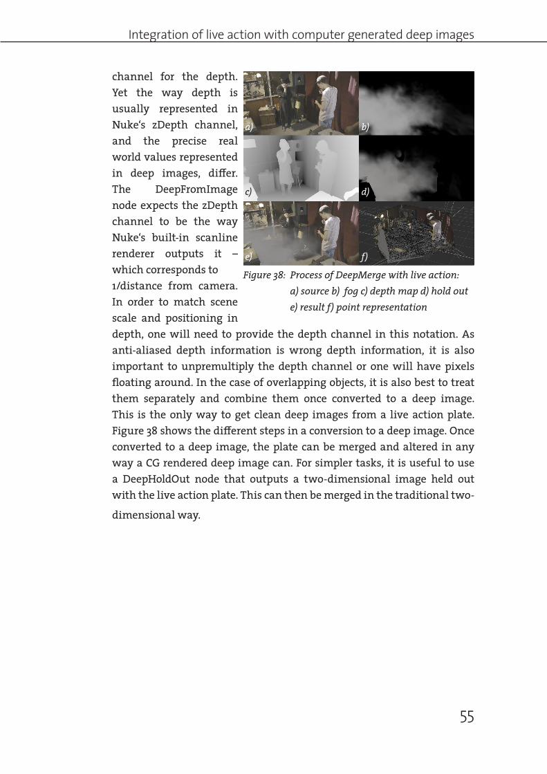
Integration of live action with computer generated deep images

55

channel for the depth. Yet the way depth is usually represented in Nuke‘s zDepth channel, and the precise real world values represented in deep images, differ. The DeepFromImage node expects the zDepth channel to be the way Nuke‘s built-in scanline renderer outputs it – which corresponds to 1/distance from camera. In order to match scene scale and positioning in depth, one will need to provide the depth channel in this notation. As anti-aliased depth information is wrong depth information, it is also important to unpremultiply the depth channel or one will have pixels floating around. In the case of overlapping objects, it is also best to treat them separately and combine them once converted to a deep image. This is the only way to get clean deep images from a live action plate. Figure 38 shows the different steps in a conversion to a deep image. Once converted to a deep image, the plate can be merged and altered in any way a CG rendered deep image can. For simpler tasks, it is useful to use a DeepHoldOut node that outputs a two-dimensional image held out with the live action plate. This can then be merged in the traditional two-

dimensional way.

Figure 38: Process of DeepMerge with live action: a) source b) fog c) depth map d) hold out e) result f) point representation

a)

c)

b)

d)

e) f)

Outlook

56

7 Outlook

All the aspects mentioned up to this point are the fundamental aspects of deep image compositing. This is what is possible out of the box until today. Looking deeper however, it becomes obvious that the additional depth information allows for far more. Combined with other data available to the compositing artist, additional possibilities start to arise permitting a much more efficient and flexible workflow. The more information is being provided in the image files, the more missing information can most likely be calculated. Giving the compositing artist information gives him the power to quickly change many aspects of the final image and allows him to apply client‘s change orders instantly without the large burden of a CG rendering.In the following chapter, I‘m going to introduce some additional options that can become possible with the installment of a deep compositing pipeline.

Deep Object IDs

A compositing artist often needs to alter individual parts of images and objects. Usually these areas are defined manually by drawing mattes for the corresponding areas. As the information about an object is already available for computer generated imagery, this matte generation can be automated. This leads to much more precise mattes and a lot less work. These Object IDs are usually rendered out as colored images where each element has a different color. Yet, since every color is described by an amount of red, green and blue, semitransparent edges often get

contaminated with other colors. Therefore, often only red, green and blue are used which limits the amount of mattes per layer to 3. Deep images now allow, due to their spatial separation of overlapping samples, every color as an object ID. This greatly increases flexibility as a large amount of

Figure 39: a) rendering, b) object ID pass c) isolated object

a) b) c)

Vector blur that works for overlapping objects

57

mattes can be rendered by default rather than only rendering important parts. This avoids big file sizes. The combination of deep images with object IDs then allows for a distinct selection of specific objects and elements even if they overlap other objects in semitransparent areas.

Vector blur that works for overlapping objects

Vector blur is often used to achieve a cheap „fake“ motion blur in compositing without the need of calculating sub-frames. To apply a vector blur, a vector pass has to be rendered from the 3D package. This usually consists of any x component of the velocity from the point of view of the camera stored in the red channel and the y component of the velocity stored in the green channel. This vector pass then drives a directional blur that, dependent on the direction and magnitude, blurs every pixel independently mimicking a motion blur. This works well for single objects that have translation in x and y only. However, for more complicated transformations and overlapping objects, it fails27. The only real solution is to render it directly in the 3D package.As outlined so far, the benefits of deep compositing lie in solving problems caused by overlapping objects. So it should help with Vector blur as well. Using a deep vector pass and a deep image, we should be able to do the directional blur separately for every depth, therefore allowing for a realistic blurring. Only the moving object would be blurred and not anything that overlaps. Still, this would expose holes behind the object which gets semitransparent due to the blur. As it was an opaque object, the ray tracing algorithm didn‘t continue; therefore, no additional depth samples were created, leaving behind a hole. Of course, rendering these objects separately would also resolve the problem; but in case this is not possible, or advisable, the above solution could make sense.So to make use of a deep vector blur, more would need to be rendered than seen through the camera. With this overlap, a true representation of a motion blur of overlapping objects could be achieved. To avoid exploding render times and file sizes, the amount of overlap could be derived from the shutter and maximum velocity.

As seen by some examples above, it is reasonable to render deep utility passes. These rendered deep utility passes usually include detailed information that should be unbiased in order to allow for a correct use in

27 c.f. Spears, D. in Okun & Zwerman. 2010. p.687

Outlook

58

compositing. With the findings concluded above, it is indisputable to say that the additional memory needed to store the passes is negligible, at least for non volumetric imagery, and especially given the value it adds.

Deep Mattes

Mattes are a fundamental part of compositing. Whether it is to cut out parts of an image or to grade only a specific area, mattes are always used in compositing. In order to work effectively with deep images, there needs to be a way of using three-dimensional mattes, similar to a world position pass, where it is easy to use geometric primitives to mask a particular region. The advantage of masks generated with a world position pass is that the masks are consistent throughout different shots as they are expressed in absolute world coordinates. This allows for a very effective masking that can be adopted to all shots of a specific setup. With deep images and, especially with the use of volumetric effects, this becomes even more handy, as volumetrics can be further shaped and adapted to the scene. There are two different ways to implement such masking features into Nuke. The first is to calculate the world space coordinates of a deep image and then compare them, similar to what was already done with world position pass masks, with a mathematical representation of the corresponding geometric primitive. The other option is to transform the geometric primitive into a deep image with the deep.front value being the point where a theoretical eye ray enters the object and the deep.back where the ray would exit the object again. A traditional zBuffer algorithm can easily be modified to save a deep zBuffer. „The z value of any new point to be written into the buffer is compared with the z value of the point already there. If the new point is behind, it is discarded. If it is in front, it replaces the old value.“28

Instead of using a two-dimensional buffer, we use a deep buffer that, like the deep image buffer, stores an arbitrary list of samples per pixel. Further, instead of discarding a value, if its z value is inferior, we simply append it to the list. To build a volumetric representation of a geometry, contiguous samples then have to be checked for their object affiliation. Moreover, it has to be determined if a sample is an entry or an exit sample. This can be achieved by setting a flag on every sample of a common mesh. The first sample will get the flag set to entry and the following samples will simply invert the flag. If the first sample isn‘t an entry sample however,

28 Catmull, E.E. 1974. p. 32

Altering the look of volumetric renderings in compositing

59

the algorithm has to be adapted. This could be achieved by checking the first sample‘s normal direction. The advantage in using a zBuffer algorithm, instead of a ray tracing algorithm, is speed. And since any light calculation is unnecessary for this application, we can easily ignore this drawback of zBuffering. A fall-off could be achieved by using multiple samples, that could then have different alpha values. This could then simply be multiplied with the image that is to be masked. The advantage of the latter method is that it would not be restricted to the use of geometric primitives but could use any kind of deep image as an input. Using such a deep mask for a deep color correction would open up many new possibilities. But the universality of absolute world coordinates would be lost, hence limiting the convenience to adopt a mask to another shot. On the other hand, any conversion between camera space and world space always implies computation on all samples. Avoiding this will result in higher performance. The transformation from geometric primitives in world space to camera space only has to be done once and can be precomputed. Whereas converting a deep image to world space and back would be one additional transformation and it would be inefficient to precompute it. Since a matte is applied more often than it is generated, saving performance on this operation helps to increase the overall processing time of a compositing script.

Altering the look of volumetric renderings in compositing

With volumetric effects and particle simulations, the look is often created by tweaking colors and opacity. However, as the different particles and voxels overlap in space, the volume can only be shaped before the rendering process. With the introduction of deep image compositing new possibilities arise. With the full color and transparency information for every point in space, the shaping and look development of volumetric effects, such as smoke and fire, can be achieved in compositing. This allows for much greater flexibility and the possibility to tweak the appearance of the effect to integrate it with the other elements. With the clear separation of spatially independent particles or volume segments, it is now possible to render any kind of information about the state of the particles or fluids into an additional channel. Information like velocity, age, temperature or any other arbitrary parameter can be incorporated and, especially, distinctly retrieved in compositing. The added flexibility and possibilities

Outlook

60

resulting from this are immense. This valuable information allows the compositing artist to substantially change the appearance of the effect without the need to re-render anything. It basically corresponds to making available a point cache of the simulated particles/volume from a camera viewpoint, to the compositing artist. As discussed earlier, the 3D department moves more into asset creation, leaving visual designing to compositing and/or look development.In order to use techniques like temperature based color corrections of volumetric effects, a second implementation for mattes is needed that greatly resembles the way mattes are used in traditional two-dimensional compositing. The concept behind this is that one wants to use additional objects describing a specific state of a certain sample. In this context, it can be assumed that both images share the same depth samples/depth values, as the represented object is the same. Usually, this information is saved in additional channels. But, due to performance issues, there might as well be separate images. The goal is to manipulate the rgba channels of the image as a function of the values in another channel/image. This function should be easily adjustable by the compositing artist. The best way would be a look up curve that graphs the dependencies between the mask input and the output of the image.

Volume fog in Comp

Fog and dust are natural phenomenons that influence the visual perception considerably. The desaturation over depth is a depth clue for the human brain, allowing us to perceive and identify three-dimensional relations. The importance of mimicking this behavior when integrating computer generated elements into photographic plates is evident. Volume fog can be rendered from a 3D package or be faked with grading later-on in compositing. With deep images, we‘re able to either use some kind of depth shader that is easily applied at the transformation from a deep image to a traditional flat image. Such a dependency can easily be inserted in the sampling process that converts a deep image to a traditional image. Like this, any parameter could be made depth dependent – even allowing for atmospheric distortion over depth.For more complex fog structures, a fog volume can either be created in a 3D application or directly and interactively in the compositing application. Using a four-dimensional noise as basis or the DeepFromFrames and a Noise as input would allow for the interactive creation of clouds, and

Light interaction

61

alike, on the fly during compositing.

Light interaction

As mentioned before, limitations come as soon as a light interaction with an object or, even more dramatic, a volume, changes. The rendered deep image has the illumination baked in and hence needs to be re-rendered. With traditional renderings, this problem is avoided by rendering light independently from the object and combining it in compositing. This is also possible, to some degree, for hard surface deep images. For volumes, however, this can‘t be done, at least not in the traditional way. „Camera Space Volumetric Shadow Maps“29 describes Weta Digital‘s approach to separate deep image volumetrics and shadows. As discussed earlier, volume intersections allow for the use of deep images as spatial mattes. This can be used to calculate light interaction with volumes and is often needed to mimic atmospheric lights also known as „god rays“. The real solution up to now was to render it in a 3D package which was very time expensive. With a volumetric deep image and a representation of light which is basically not much more than a fall-off if it isn‘t occluded, we can now easily multiply both and get interactive volumetric light in compositing. For more complex light situations, a workflow as the one described in „Camera Space Volumetric Shadow Maps“ can be used. The concept basically involves rendering light rays as deep image in camera space instead of in light space. In combination with simple volume representation created in the compositing package, as mentioned above, this allows for the interactive creation of volumetric lights in compositing.

Building a deep image library

Since render times are precious, it seems logical to use deep compositing to build up an element library. The advantage over traditional images for library use is clearly apparent. Instead of only being able to use rendered elements as classical live action elements, and thus being limited to use in the background, a deep image library would consist of elements that permit an interaction with other objects, even after rendering. Like this, they can be used in a much broader way without the downside of classic elements that look flat and 2D because of missing depth integration, and they avoid the bulk of excessive render times for volumetric effects.

29 Hanika, J., Hillman, P., Hill, M., Fascione, L. 2012

Outlook

62

As seen in prior chapters, the world space location of depth samples can be calculated. With this in mind one quickly dreams of interactively changing camera positions to accommodate shot specific needs for elements, or even fly through a single deep image. Still there are some aspects that unfortunately complicate this. One is the fact that as soon as full opacity is reached, no further samples are gathered. The missing information from occluded objects might thus be revealed by a change of the camera angle. This can definitely be accommodated for by rendering occluded objects, continuing ray tracing/ray marching even after an opaque object is reached or after a point of full opacity. Yet this means increased computation and thus increased render times. A second aspect is that in order to represent the pixel samples from a differing angle of view, some kind of voxel rendering engine is needed. As this involves true rendering again, I would abandon that idea and rather encourage building a library of simulated volumetric effects as point caches and re-render them in times of need for a specific camera angle and/or move.It is also clear that such a library won‘t be able to provide elements for every single shot as the specific requirements will vary. As soon as further interaction is needed that would alter the effect in itself again, there is no way around a complete new simulation. Light changes can be dealt with up to a certain degree as discussed previously. Still, I‘m convinced that certain effects can be used as library elements and provide value over the use of traditional elements because of the possibility of creating holdout mattes on the fly. This is true for a large amount of volumetric effects as well as for particle effects such as rain, confetti etc. Instead of layering different plates that would still look layered because occlusion wouldn‘t match 100%, we can get a realistic placement of our character in the particles. This is especially important for stereoscopic productions where two-dimensional cheating doesn‘t work.

Stereo

With more and more stereoscopic movies finding their way into theaters, their impact on the visual effects industry is tremendous. It does not only mean doing the work twice for the two different eyes, but it also means that old tricks that were established over the years and have worked well for over a decade, can‘t be used anymore. Cheating that would not be visible on traditional 2D movies now suddenly becomes apparent. This

Stereo

63

means that a lot of work has to be highly exact and three-dimensionally correct. Having exact depth information in compositing, in order to holdout computer generated elements, is a huge advantage. It is much easier to adjust depth of a holdout matte in compositing because the depth in relation to the elements in the plate can be exactly matched and verified.Another important point is that layering is not effective any more, it appears flat. Gaining additional depth becomes important when it comes to stereoscopic images. Deep images present a good way of keeping depth and flexibility.

65

8 Conclusion

Deep compositing brings many benefits, two of them particularly worth mentioning. The first is increased flexibility which is demonstrated by its capability to render elements independently and combine them in compositing. The second is the unbiased depth and color information that deep images present. With this, artefacts caused by inaccurate depth information are eliminated. As with every good tool, deep compositing allows the artist to become even more creative, removing technical headaches posed by structural restrictions.However, these advantages come at a price – decreased performance. Especially for volumetric renderings, file sizes can explode and present a big processing challenge. Therefore, deep images should not be used blindly. Not every situation needs the additional depth information. The relation of file size to information is linear, the larger the files are, the more information they contain. However, more information does not always mean a better result. Some situations do not require as much depth resolution, so it is better to keep the file sizes reasonable. Additionally, handling of large deep images can be optimized by using concepts such as proxies and region of interest. Volumetric renderings may result in the largest files but they also bring a huge advantage. And although non-volumetric renderings don‘t have as big an impact on performance, they still offer reasonable benefits over traditional images in semi-transparent areas.Before deep compositing is used in production, the infrastructure must be tested and, if necessary, adapted to facilitate a flawless adoption of deep compositing. Otherwise, the use of deep images can cause serious decline in performance and a potential breakdown of the network infrastructure.Still, this is only the beginning. There is great potential in deep images but the tools to handle them are sparse. This will hopefully change with the official release of a standard format, namely Open EXR 2.0. In this context, I would like to advocate for a further standardization to save the camera matrix in the meta data. This essential information is needed by many tools, and should be clearly and distinctly embedded into the image itself. The possibilities offered by deep images will increase greatly once the tools evolve. The lines between 3D and compositing will get ever more blurred, introducing more and more possibilities and flexibility. This will potentially lead to a future of voxel based compositing, where the image is not the intermediate, but only the final product.

66

Acknowledgments

I wish to thank Prof. Katja Schmid and Michael Landgrebe for their great assistance with my work. My special thanks are extended to Holger Hummel, Justin Daneman and all the other great people at Celluloid VFX who were a great help and provided an exeptional work atmosphere during my research. I am grateful to Vladimir Koylazov from Chaos Group and Colin Doncaster from Peregrine Labs who provided me Software and in depth technical knowledge. Advice given by Johannes Saam, Jonathan Egstad, Peter Pearson, Denis Scolan, Ivan Busquets and every one else on the Nuke mailinglist has been a great help. Assistance provided by Sebastian Elsner and Oliver Hohn was greatly appreciated. My thanks to Stefan Seibert, who wrote plugins to validate my ideas. I would also like to acknowledge the support provided by my family during the writing.

67

Appendix A – References

Okun, J. A. & Zwerman, S. 2010. The VES Handbook of Visual Effects. Elsevier

Lokovic, T. and Veach, E. 2000. Deep Shadow Maps. SIGGRAPH Comput. Graph.,385-392

Heckenberg, D., Saam, J., Doncaster, C., Cooper, C. 2010. Deep Compositing www.johannessaam.com/deepImage.pdf (accessed 17.03.2013)

Kainz, F., and Bogart, R. 2011. Technical Introduction to OpenEXR. https://github.com/openexr/openexr/blob/master/OpenEXR/doc/TechnicalIntroduc-tion_2.0.pdf (accessed 17.03.2013)

Harvey, V., Brady, A., Ring, D., Binks, J., Wadelton, J., Hughes, M. 2013. NDK De-veloper Guide http://docs.thefoundry.co.uk/nuke/70/ndkdevguide/in-tro/intro.html (accessed 17.03.2013)

Akenie-Möller, T., Haines, E.,Hoffman, N. 2008. Real-Time Rendering Third Editi-on. A K Peters

Shannon, C.E. 1948. A Mathematical Theory of Communication. Bell System Technical Journal, Vol. 27, pp. 379–423, 623–656

Ziv, J., and Lempel, A. 1977. A universal algorithm for sequential data compression, IEEE Transactions on Information Theory, v.23 n.3, p.337-343

Feldspar, A. 1997. An Explanation of the Deflate Algorithm. www.zlib.net/feld-spar.html (accessed 17.03.2013)

Wehmeier S. 2000. Oxford Advanced Learner‘s Dictionary of Current English. Oxford University Press

Catmull, E.E. 1974. A Subdivision Algorithm for Computer Display of Curved Surfa-ces. The University of Utah

Hanika, J., Hillman, P., Hill, M., Fascione, L. 2012. Camera Space Volumetric Shadows. DigiPro‘12 p. 7-14

68

Appendix B – List of Figures

Figure 1: An illustration of the sample gathering proess 10Figure 2: Antialiased(left) and aliased(right) edge 12Figure 3: zMerge: Merge of a) and b), c) unfiltered, d) filtered, e) DeepMerge 13Figure 4: a) zBlur b) Frischluft c) Bokeh 14Figure 5: a) deep rgba b) deep alpha c) zDepth 15Figure 6: A refracting object with the backgrond cropped 16Figure 7: Teapots(a) get merged with fog (c) traditional holdout(b), d) and e) show

the possibility to rearrange in compositing 17Figure 8: removing the object in a) reveals a hole(b) 17Figure 10: A world position pass(left) and a matte created from it (right) 18Figure 9: merging the cubes left and right produces a rough edge (middle) 18Figure 11: settings for the stereoscopic helper 20Figure 12: Point representation of a cube(left) and the same with DeepTransform

with noise as mask applied(right) 22Figure 13: Result of a DeepColorCorrect restricted to a specific depth slice 23Figure 14: Output of the DeepToPoints node 24Figure 15: Relations between points in 3D space and their projection onto a 2D

plane 25Figure 16: Control panel of the DeepSample node 28Figure 17: Depth graph with a single pixel sampled (top) and a region sampled

(bottom) 29Figure 18: The distorted result of DeepToPoints (left) and the correct result

(right) 30Figure 19: Relation of sample count and uncompressed filesize 32Figure 20: Bit depth of the elements that make up an OpenEXR 2.0 deep image 33Figure 21: a) Fur rendering, b) pixels with more than one sample, c) sample count

represented as the height of layers 34Figure 22: Total bits per file and the corresponding repartion of the channels 35Figure 23: performance monitoring of a VRay rendering (fur) 36Figure 24: Performance monitoring VRay rendering (smoke) 36Figure 25: Performance of a Nuke rendering 37Figure 26: Performance of a Nuke rendering, smoke sequence 38Figure 27: Performance comparison of server, local HDD and local SSD 39Figure 28: Performance of a Nuke rendering, reading and writing a deep file 40Figure 29: Network trafic (write bytes) of the server 41Figure 30: Examplary performance of a render node (top) and reference of the

same (bottom) 41

69

Figure 31: Processor time and bytes sent/sec and fall symultaneously to the write bytes on the server 42

Figure 32: Write Bytes/sec on the server during a Nuke network rendering 43Figure 33: Performance during an examplary frame on a network rendering(top)

and single rendering (bottom) 44Figure 34: Building a Huffman tree 46Figure 35: Fire rendering, deep 50Figure 36: File size, rendertime and sample count of an original and a proxy 53Figure 37: Node construct for a deep region of interest 53Figure 38: Process of DeepMerge with live action: a) source b) fog c) depth map

d) hold out e) result f) point representation 55Figure 39: a) rendering, b) object ID pass c) isolated object 56

70

Appendix C – Nuke bug list

#31474 DeepRead width and height via Python return root formatUsing Python to read out the width and height of a DeepRead node(n.width() with n beeing the DeepRead), width and height of the rootformat and not of the DeepRead node are returned.

#27372 Expand the functionality of the DeepExpression node to match the regularExpression node.

#32583 Feature Request: Scanline renderer deep outputThe scanline renderer should output deep data.

#32759 DeepWrite compressionOnly Zip(1 Scanline), is supported for deep EXRs. In that case the dropdown shouldonly have that option.

#32819 isDeepFilename() should spot EXRs that have deep dataThe isDeepFilename() in nukescripts/create should be adapted to spotEXRs that have deep data. As Drag and drop and the „R“ shortcut failotherwise, defaulting to a normal Read node instead of DeepRead.

#32828 node.channels() on deep nodes returns []When calling node.channels() on a deep node an empty list is returned instead ofthe channels one gets with a normal IOP node.

#32859 deep image: copied layers don‘t show in viewerWhen copying rgba from a deep image to a custom layer(e.g. layer 1) with aDeepExpression node, it will copy the values but won‘t be visible in theviewer, when selecting layer1.

#33184 distorted pointcloud in DeepToPoints The pointcloud from DeepToPoints gets distorted if the bbox of the image differsfrom the format.

71

#34208 Feature Request: Visualization of Deep VolumesA representation, e.g. streaks instead of points for volumetric samples, that alowto distiguish these and to evaluate their depth is strongly encouraged.

#34492 Error loading EXR 2.0 bigger than 2GB (on Windows)Writing out 16bit half Zip(scanline) deep EXRs(2.0) from Nuke and loading themback-in with the DeepRead, one of the following error messages appears if the fileis larger than 2048 MB:

DeepRead1: Invalid argument.DeepRead1: Error reading sample count data from file“...“. Unexpected end of file.DeepRead1:Domain Error.DeepRead1:No such file or directory.

Deep image compositing in a modern visual effects pipeline.€¦ · Nuke and VRay/3ds Max will be...

Documents

Transcript of Deep image compositing in a modern visual effects pipeline.€¦ · Nuke and VRay/3ds Max will be...