Deep Convolutional Neural Networks for RamanSpectrum Recognition : A Unified Solution

Jinchao Liu1, Margarita Osadchy2, Lorna Ashton3, Michael Foster4,Christopher J. Solomon1,5, and Stuart J. Gibson?1,5

1VisionMetric Ltd, Canterbury, Kent, UK2Department of Computer Science, University of Haifa, Mount Carmel, Haifa, Israel

3Department of Chemistry, Lancaster University, Bailrigg, Lancaster, UK4IS-Instruments Ltd. 220 Vale Road, Tonbridge, Kent, UK

5University of Kent, Canterbury, Kent, UK

Abstract

Machine learning methods have found many applications in Raman spectroscopy, espe-cially for the identification of chemical species. However, almost all of these methods re-quire non-trivial preprocessing such as baseline correction and/or PCA as an essential step.Here we describe our unified solution for the identification of chemical species in which aconvolutional neural network is trained to automatically identify substances according totheir Raman spectrum without the need of ad-hoc preprocessing steps. We evaluated ourapproach using the RRUFF spectral database, comprising mineral sample data. Superiorclassification performance is demonstrated compared with other frequently used machinelearning algorithms including the popular support vector machine.

1 Introduction

Raman spectroscopy is a ubiquitous method for characterisation of substances in a wide rangeof se�ings including industrial process control, planetary exploration, homeland security, lifesciences, geological field expeditions and laboratory materials research. In all of these environ-ments there is a requirement to identify substances from their Raman spectrum at high ratesand o�en in high volumes. Whilst machine classification has been demonstrated to be an essen-tial approach to achieve real time identification, it still requires preprocessing of the data. Thisis true regardless of whether peak detection or multivariate methods, operating on whole spec-tra, are used as input. A standard pipeline for a machine classification system based on Ramanspectroscopy includes preprocessing in the following order: cosmic ray removal, smoothing andbaseline correction. Additionally, the dimensionality of the data is o�en reduced using principal

1

arX

iv:1

708.

0902

2v1

[cs

.LG

] 1

8 A

ug 2

017

components analysis (PCA) prior to the classification step. To the best of our knowledge, thereis no existing work describing machine classification systems that can directly cope with rawspectra such as those a�ected significantly by baseline distorsion.

In this work we focus on multivariate methods, and introduce the application of convolu-tional neural networks (CNNs) in the context of Raman spectroscopy. Unlike the current Ra-man analysis pipelines, CNN combines preprocessing, feature extraction and classification ina single architecture which can be trained end-to-end with no manual tuning. We show thatCNN not only greatly simplifies the development of a machine classification system for Ramanspectroscopy, but also achieves significantly higher accuracy. In particular, we show that CNNtrained on raw spectra significantly outperformed other machine learning methods such as sup-port vector machine (SVM) with baseline corrected spectra. Our method is extremely fast witha processing rate of one sample per millisecond 1.

The baseline component of a Raman spectrum is caused primarily by fluorescence, can bemore intense than the actual Raman sca�er by several orders of magnitude, and adversely a�ectsthe performance of machine learning systems. Despite considerable e�ort in this area, baselinecorrection remains a challenging problem, especially for a fully automatic system[1].

A variety of methods for automatic baseline correction have been used such as polynomialbaseline modelling[1], simulation-based methods[2, 3], penalized least squares[4, 5]. Lieber etal.[1] proposed a modified least-squares polynomial curve fi�ing for fluorescence substractionwhich was shown to be e�ective. Eilers et al.[6] proposed a method called asymmetric least squaresmoothing. One first smooths a signal by a Whi�aker smoother to get an initial baseline esti-mation, and then applies asymmetric least square fi�ing where positive deviations with respectto baseline estimate are weighted (much) less than negative ones. This has been shown to be auseful method, and in principle can be used for automatic baseline correction, although it mayoccasionally require human input. Kneen et al.[2] proposed a method called rolling ball. In thismethod one imagines a ball with tunable radius rolling over/under the signal. The trace of itslowest/highest point is regarded as an estimated baseline. A similar methods is rubber band[3]where one simulates a rubber band to find the convex hull of the signal which can then be used asa baseline estimation. Zhang et al.[4] presented a variant of penalized least squares, called adap-tive iteratively reweighted Penalized Least Squares (airPLS) algorithm. It iteratively adapts weightscontrolling the residual between the estimated baseline and the original signal. A detailed reviewand comparison of baseline correction methods can be found in Schulze et al.[7].

Classification rates have been compared for various machine learning algorithms using Ra-man data. The method that is frequently reported to outperform other algorithms is supportvector machines (SVM) [8]. An SVM is trained by searching for a hyperplane that optimally sep-arates labelled training data with maximal margin between the training samples and the hyper-plane. Binary (two class) and small scale problems in Raman spectroscopy have been previouslyaddressed using this method. A large proportion of these relate to applications in the healthsciences, use a non-linear SVM with a radial basis function kernel, and an initial principal com-

1So�ware processing time only. Not including acquisition of Raman signal from spectrometer.

2

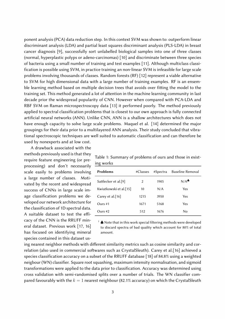
ponent analysis (PCA) data reduction step. In this context SVM was shown to: outperform lineardiscriminant analysis (LDA) and partial least squares discriminant analysis (PLS-LDA) in breastcancer diagnosis [9], successfully sort unlabelled biological samples into one of three classes(normal, hyperplastic polyps or adeno-carcinomas) [10] and discriminate between three speciesof bacteria using a small number of training and test examples [11]. Although multiclass classi-fication is possible using SVM, in practice training an non-linear SVM is infeasible for large scaleproblems involving thousands of classes. Random forests (RF) [12] represent a viable alternativeto SVM for high dimensional data with a large number of training examples. RF is an ensem-ble learning method based on multiple decision trees that avoids over fi�ing the model to thetraining set. This method generated a lot of a�ention in the machine learning community in lastdecade prior the widespread popularity of CNN. However when compared with PCA-LDA andRBF SVM on Raman microspectroscopy data [13] it performed poorly. The method previouslyapplied to spectral classification problems that is closest to our own approach is fully connectedartificial neural networks (ANN). Unlike CNN, ANN is a shallow architectures which does nothave enough capacity to solve large scale problems. Maquel et al. [14] determined the majorgroupings for their data prior to a multilayered ANN analysis. Their study concluded that vibra-tional spectroscopic techniques are well suited to automatic classification and can therefore beused by nonexperts and at low cost.

Table 1: Summary of problems of ours and those in exist-ing works

Problems #Classes #Spectra Baseline Removal

Sa�lecker et al.[9] 2 1905 N/A♣

Kwiatkowski et al.[15] 10 N/A Yes

Carey et al.[16] 1215 3950 Yes

Ours #1 1671 5168 Yes

Ours #2 512 1676 No

1 ♣Note that in this work special filtering methods were developedto discard spectra of bad quality which account for 80% of totalamount.

A drawback associated with themethods previously used is that theyrequire feature engineering (or pre-processing) and don’t necessarilyscale easily to problems involvinga large number of classes. Moti-vated by the recent and widespreadsuccess of CNNs in large scale im-age classification problems we de-veloped our network architecture forthe classification of 1D spectral data.A suitable dataset to test the e�i-cacy of the CNN is the RRUFF min-eral dataset. Previous work [17, 16]has focused on identifying mineralspecies contained in this dataset us-ing nearest neighbor methods with di�erent similarity metrics such as cosine similarity and cor-relation (also used in commercial so�wares such as CrystalSleuth). Carey et al.[16] achieved aspecies classification accuracy on a subset of the RRUFF database [18] of 84.8% using a weightedneigbour (WN) classifier. Square root squashing, maximum intensity normalisation, and sigmoidtransformations were applied to the data prior to classification. Accuracy was determined usingcross validation with semi-randomised splits over a number of trials. The WN classifier com-pared favourably with the k = 1 nearest neighbour (82.1% accuracy) on which the CrystalSleuth

3

Figure 1: Diagram of the proposed CNN for spectrum recognition. It consists of a number ofconvolutional layers for feature extraction and two fully-connected layer for classification.

matching so�ware is believed to be based. In Table 1 we summarise the sample data used in ourown work and in some previous Raman based spectral classification studies.

2 Materials and Methods

CNNs have become the predominant tool in a number of research areas - especially in computervision and text analysis. An extension of the artificial neural network concept [19], CNNs arenonlinear classifiers that can identify unseen examples without the need for feature engineering.They are computational models[20] inspired by the complex arrangement of cells in the mam-malian visual cortex. These cells are stimulated by small regions of the visual field, act as localfilters, and encode spatially localised regions of natural signals or images.

CNNs are designed to extract features from an input signal with di�erent levels of abstrac-tion. A typical CNN includes convolutional layers, which learn filter maps for di�erent typesof pa�erns in the input, and pooling operators which extract the most prominent structures.The combination of convolutional and pooling layers extracts features (or pa�erns) hierarchi-cally. Convolutional layers share weights which allow computations to be saved and also makethe classifier invariant to spatial translation. The fully connected layers (that follow the convo-lutional and pooling layers) and the so�max output layer can be viewed as a classifier whichoperates on the features (of the Raman spectra data), extracted using the convolutional andpooling layers. Since all layers are trained together, CNNs integrate feature extraction with clas-sification. Features determined by network training are optimal in the sense of the performance

4

of the classifier. Such end-to-end trainable systems o�er a much be�er alternative to a pipelinein which each part is trained independently or cra�ed manually.

In this work, we evaluated the application of a number of prominent CNN architecturesincluding LeNets[21], Inception[22] and Residual Nets[23] to Raman spectral data. All threeshowed comparable classification results even though the la�er two have been considered su-perior to LeNet in computer vision applications. We adopted a variant of LeNet, comprisingpyramid-shaped convolutional layers for feature extraction and two fully-connected layers forclassification. A graphical illustration of the network is shown in Figure 1.

2.1 CNN for Raman Spectral Data Classification

The input to the CNN in application to Raman spectrum classification is one dimensional and itcontains the entire spectrum (intensity fully sampled at regularly spaced wavenumbers). Hencewe trained one-dimensional convolutional kernels in our CNN. For the convolutional layers, weused LeakyReLU[24] nonlinearity, defined as

f(x) =

{x, if x > 0

ax, otherwise(1)

Formally, a convolutional layer can be expressed as follows:

yj = f

(bj +

∑i

kij ∗ xi)

(2)

where xi and yi are the i-th input map and the j-th output map, respectively. kij is a convolu-tional kernel between the maps i and j, ∗ denotes convolution, and bj is the bias parameter ofthe j-th map.

The convolutional layer is followed by a max-pooling layer, in which each neuron in theoutput map yi pools over an s× s non-overlapping region in the input map xi. Formally,

yij = max0≤m<s

{xij·s+m} (3)

The upper layers of the CNN are fully connected and followed by the so�max with the num-ber of outputs equal to the number of classes considered. We used tanh as non-linearity inthe fully connected layers. The so�max operates as a squashing function that re-normalizesa K-dimensional input vector z of real values to real values in the range [0, 1] that sum to 1,specifically,

σ(z)j =ezj∑Kk=1 e

zkfor j = 1, ..., K. (4)

To avoid overfi�ing the model to the data, we applied batch normalization [25] a�er eachlayer and dropout [26] a�er the first fully connected layer. Further details of the architectureare shown in Figure 1.

5

2.2 CNN Training

Since the classes in the our experiments have very di�erent numbers of examples, we used thefollowing weighted loss to train the CNN:

L(w, xn, yn) = −1

N

N∑n=1

αn

K∑k=1

tkn ln ykn (5)

where xn is a training spectrum, tn is the true label of the nth sample in the format of one-hotencoding, yn is the network prediction for the nth sample, αn ∝ 1

#Cand #C is the number of

samples in the classC that xn belongs to. N is the total number of samples andK is the numberof the classes.

CNN is a data hungry model. To reduce the data volume requirements we use augmentationwhich is a very common approach for increasing the size of the training sets for CNN training.Here, we propose the following data augmentation procedure: (1) We shi�ed each spectrumle� or right a few wavenumbers randomly. (2) We added a random noise, proportional to themagnitude at each wave number. (3) For the substances which had more than one spectra, wetook linear combinations of all spectra belonging to the same substance as augmented data. Thecoe�icients in the linear combination were chosen at random.

The training of the CNN was performed using Adam algorithm [27], which is a variant ofstochastic gradient descent, for 50 epochs with learning rate equal to 1e-3, β1 = 0.9, β2 = 0.999,and ε=1e-8. The layers were initialised from a Gaussian distribution with a zero mean and vari-ance equal to 0.05. We applied early stopping to prevent overfi�ing. Training was performed ona single NVIDIA GTX-1080 GPU. The training time was around seven hours. While for inference,it took less than one millisecond to process a spectrum.

2.3 Evaluation Protocol

We tested the proposed CNN method for mineral species recognition on the largest publiclyavailable mineral database RRUFF[18] and compared it with a number of alternative, well known,machine learning methods. As there are usually only a handful of spectra available for each min-eral, we use a leave-one-out scheme to split a dataset into training and test sets. To be specific,for minerals which have more than one spectra, we randomly select a spectrum for testing anduse the rest for training. We compared our method to cosine similarity [16]/correction [15](which has been used in commercial so�ware such as CrystalSleuth and Spectral-ID), and toother methods that have been shown to be successful in classification tasks including applica-tions based on Raman: nearest neighbor, gradient boosting machine, random forest, and supportvector machine[28].

The proposed CNN was implemented using Keras[29] and Tensorflow[30]. The gradientboosting machine method was implemented based on lightGBM released by Microso�. All othermethods were implemented using on Scikit-learn[31].

6

Table 2: Test accuracy of the compared machine learning methods on the baseline correcteddatasetMethods KNN(k=1) Gradient

BoostingRandomForest†

SVM(linear) SVM(rbf) Correlation CNN†

Top-1 Accuracy 0.779±0.011 0.617±0.008 0.645±0.007 0.819±0.004 0.746±0.003 0.717±0.006 0.884±0.005

Top-3 Accuracy 0.780±0.011 0.763±0.011 0.753±0.010 0.903±0.006 0.864±0.006 0.829±0.005 0.953±0.002

Top-5 Accuracy 0.780±0.011 0.812±0.010 0.789±0.009 0.920±0.003 0.890±0.007 0.857±0.005 0.963±0.002

3 Results and Discussion

3.1 Classifying baseline-corrected spectra

We first evaluated our CNN method on a processed mineral dataset from the RRUFF database.These spectra have been baseline corrected and cosmic rays have also been removed. The datasetcontains 1671 di�erent kinds of minerals, 5168 spectra in total. Spectra for the mineral Actinoliteis shown in Figure 2(a), illustrating the typical within-class variance. The number of spectra permineral ranges from 1 to 40. The distribution of sample numbers per a mineral species is shownin Figure 2(b). We followed the protocol as described in Section 2.3 to generate training and testsets randomly using the leave-one-out scheme.

In a large scale classification, some classes could be quite similar and di�erentiating betweenthem could be very di�icult or even impossible. Hence, it is common to report top-1 and top-kaccuracy. In the former, the class that the classifier assigns the highest probability to is comparedto the true label. The la�er reports whether the true label appears among the k classes with thehighest probability (assigned by the classifier).

We report in Table 2, the top 1, 3 and 5 accuracies of the compared methods, averaged over50 independent runs. One can see that CNN significantly outperformed all other methods andachieved top-1 accuracy of 88.4% and top-3 accuracy of 96.3%.

0 200 400 600 800 1000 1200 1400

Raman Shift(cm−1)

0.0

0.2

0.4

0.6

0.8

1.0

Inte

nsit

y

(a) Spectra of Actinolite[18].

0 200 400 600 800 1000 1200 1400 1600Class label

0

5

10

15

20

25

30

35

Num

ber

ofSa

mpl

es

(b) Number of spectra per mineral of the whole dataset.

Figure 2: (a) Spectra of an example mineral species (Actinolite) indicating the within class spec-trum variation and (b) a frequency plot showing the imbalance regarding spectra per species.

7

0 200 400 600 800 1000 1200 1400 16000.00.20.40.60.81.0

Inte

nsit

y actinolite :test sample

0 200 400 600 800 1000 1200 1400 1600

Raman Shift(cm−1)

0.00.20.40.60.81.0

Inte

nsit

y actinolite :scores=9.34E-01

0 200 400 600 800 1000 1200 1400 1600

Raman Shift(cm−1)

0.00.20.40.60.81.0

Inte

nsit

y ferroactinolite :scores=4.62E-02

0 200 400 600 800 1000 1200 1400 1600

Raman Shift(cm−1)

0.00.20.40.60.81.0

Inte

nsit

y tremolite :scores=1.18E-02

(a) Succeeded, top-1 hit

0 200 400 600 800 1000 1200 1400 16000.00.20.40.60.81.0

Inte

nsit

y amblygonite :test sample

0 200 400 600 800 1000 1200 1400 1600

Raman Shift(cm−1)

0.00.20.40.60.81.0

Inte

nsit

y montebrasite :scores=8.98E-01

0 200 400 600 800 1000 1200 1400 1600

Raman Shift(cm−1)

0.00.20.40.60.81.0

Inte

nsit

y amblygonite :scores=5.08E-03

0 200 400 600 800 1000 1200 1400 1600

Raman Shift(cm−1)

0.00.20.40.60.81.0

Inte

nsit

y euchlorine :scores=4.79E-03

(b) Succeeded, top-3 hit

0 200 400 600 800 1000 1200 1400 16000.00.20.40.60.81.0

Inte

nsit

y russellite :test sample

0 200 400 600 800 1000 1200 1400 1600

Raman Shift(cm−1)

0.00.20.40.60.81.0

Inte

nsit

y hydrokenoelsmoreite :scores=2.65E-01

0 200 400 600 800 1000 1200 1400 1600

Raman Shift(cm−1)

0.00.20.40.60.81.0

Inte

nsit

y montroseite :scores=2.41E-02

0 200 400 600 800 1000 1200 1400 1600

Raman Shift(cm−1)

0.00.20.40.60.81.0

Inte

nsit

y whitlockite :scores=2.39E-02

(c) Failed, but similar

0 200 400 600 800 1000 1200 1400 16000.00.20.40.60.81.0

Inte

nsit

y merlinoite :test sample

0 200 400 600 800 1000 1200 1400 1600

Raman Shift(cm−1)

0.00.20.40.60.81.0

Inte

nsit

y phillipsiteca :scores=2.33E-01

0 200 400 600 800 1000 1200 1400 1600

Raman Shift(cm−1)

0.00.20.40.60.81.0

Inte

nsit

y garroniteca :scores=8.70E-02

0 200 400 600 800 1000 1200 1400 1600

Raman Shift(cm−1)

0.00.20.40.60.81.0

Inte

nsit

y phillipsitena :scores=5.97E-02

(d) Failed, partially matching

Figure 3: Examples of successful and unsuccessful mineral species classifications. In each plot,the top spectrum which is marked in red is a test sample. The three spectra below were thetop-3 predictions given by the CNN among which the correct one was highlighted in green. Theprediction scores were also shown in each plot which reflect the confidence level of predictions.

8

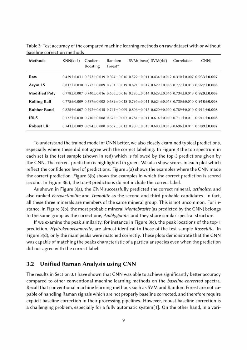
Table 3: Test accuracy of the compared machine learning methods on raw dataset with or withoutbaseline correction methods

Methods KNN(k=1) GradientBoosting

RandomForest†

SVM(linear) SVM(rbf) Correlation CNN†

Raw 0.429±0.011 0.373±0.019 0.394±0.016 0.522±0.011 0.434±0.012 0.310±0.007 0.933±0.007

Asym LS 0.817±0.010 0.773±0.009 0.731±0.019 0.821±0.012 0.629±0.016 0.777±0.013 0.927±0.008

Modified Poly 0.778±0.007 0.740±0.016 0.650±0.016 0.785±0.014 0.629±0.016 0.734±0.013 0.920±0.008

Rolling Ball 0.775±0.009 0.737±0.008 0.689±0.018 0.795±0.011 0.624±0.013 0.730±0.010 0.918±0.008

Rubber Band 0.825±0.007 0.792±0.015 0.741±0.009 0.806±0.015 0.620±0.010 0.789±0.010 0.911±0.008

IRLS 0.772±0.010 0.710±0.008 0.675±0.007 0.781±0.011 0.614±0.010 0.711±0.011 0.911±0.008

Robust LR 0.741±0.009 0.694±0.008 0.667±0.012 0.759±0.013 0.600±0.013 0.696±0.011 0.909±0.007

To understand the trained model of CNN be�er, we also closely examined typical predictions,especially where these did not agree with the correct labelling. In Figure 3 the top spectrum ineach set is the test sample (shown in red) which is followed by the top-3 predictions given bythe CNN. The correct prediction is highlighted in green. We also show scores in each plot whichreflect the confidence level of predictions. Figure 3(a) shows the examples where the CNN madethe correct prediction. Figure 3(b) shows the examples in which the correct prediction is scoredsecond. In Figure 3(c), the top-3 predictions do not include the correct label.

As shown in Figure 3(a), the CNN successfully predicted the correct mineral, actinolite, andalso ranked Ferroactinolite and Tremolite as the second and third probable candidates. In fact,all these three minerals are members of the same mineral group. This is not uncommon. For in-stance, in Figure 3(b), the most probable mineral Montebrasite (as predicted by the CNN) belongsto the same group as the correct one, Amblygonite, and they share similar spectral structure.

If we examine the peak similarity, for instance in Figure 3(c), the peak locations of the top-1prediction, Hydrokenoelsmoreite, are almost identical to those of the test sample Russellite. InFigure 3(d), only the main peaks were matched correctly. These plots demonstrate that the CNNwas capable of matching the peaks characteristic of a particular species even when the predictiondid not agree with the correct label.

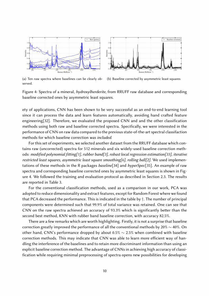
3.2 Unified Raman Analysis using CNN

The results in Section 3.1 have shown that CNN was able to achieve significantly be�er accuracycompared to other conventional machine learning methods on the baseline-corrected spectra.Recall that conventional machine learning methods such as SVM and Random Forest are not ca-pable of handling Raman signals which are not properly baseline corrected, and therefore requireexplicit baseline correction in their processing pipelines. However, robust baseline correction isa challenging problem, especially for a fully automatic system[1]. On the other hand, in a vari-

9

200 400 600 800 1000 1200

Raman Shift(cm−1)

0.0

0.2

0.4

0.6

0.8

1.0

Inte

nsit

y

Raw spectra

(a) Ten raw spectra where baselines can be clearly ob-served.

200 400 600 800 1000 1200

Raman Shift(cm−1)

0.0

0.2

0.4

0.6

0.8

1.0

Inte

nsit

y

Baseline corrected

(b) Baseline corrected by asymmetric least squares

Figure 4: Spectra of a mineral, hydroxylherderite, from RRUFF raw database and correspondingbaseline corrected ones by asymmetric least squares.

ety of applications, CNN has been shown to be very successful as an end-to-end learning toolsince it can process the data and learn features automatically, avoiding hand cra�ed featureengineering[32]. Therefore, we evaluated the proposed CNN and and the other classificationmethods using both raw and baseline corrected spectra. Specifically, we were interested in theperformance of CNN on raw data compared to the previous state-of-the-art spectral classifactionmethods for which baseline correction was included.

For this set of experiments, we selected another dataset from the RRUFF database which con-tains raw (uncorrected) spectra for 512 minerals and six widely-used baseline correction meth-ods: modified polynomial fi�ing[1], rubber band[3], robust local regression estimation[33], iterativerestricted least squares, asymmetric least square smoothing[6], rolling ball[2]. We used implemen-tations of these methods in the R packages baseline[34] and hyperSpec[35]. An example of rawspectra and corresponding baseline corrected ones by asymmetric least squares is shown in Fig-ure 4. We followed the training and evaluation protocol as described in Section 2.3. The resultsare reported in Table 3.

For the conventional classification methods, used as a comparison in our work, PCA wasadopted to reduce dimensionality and extract features, except for Random Forest where we foundthat PCA decreased the performance. This is indicated in the table by †. The number of principalcomponents were determined such that 99.9% of total variance was retained. One can see thatCNN on the raw spectra achieved an accuracy of 93.3% which is significantly be�er than thesecond best method, KNN with rubber band baseline correction, with accuracy 82.5%.

There are a few remarks which are worth highlighting. Firstly, it is not a surprise that baselinecorrection greatly improved the performance of all the conventional methods by 20%∼ 40%. Onother hand, CNN’s performance dropped by about 0.5% ∼ 2.5% when combined with baselinecorrection methods. This may indicate that CNN was able to learn more e�icient way of han-dling the interference of the baselines and to retain more discriminant information than using anexplicit baseline correction method. The advantage of CNNs in achieving high accuracy of classi-fication while requiring minimal preprocessing of spectra opens new possibilities for developing

10

highly accurate fully automatic spectrum recognition systems.

4 Conclusion and Future Work

In this paper, we have presented a deep convolutional neural network solution for Raman spec-trum classification which not only exhibits outstanding performance, but also avoids the needfor spectrum preprocessing of any kind. Our method has been validated on a large scale mineraldatabase and was shown to outperform other state-of-the-art machine learning methods by alarge margin. Although we focused our study on Raman data we believe the method is also appli-cable to other spectroscopy and spectrometry methods. We speculate that this may be acheivedvery e�iciently by exploiting basic similarities in the shape of spectra originating from di�erenttechniques and fine tuning our network to address new classification problems. This process isknown as transfer learning and has been demomstrated previously in many object recognitionapplications.

References

[1] C. A. Lieber and A. Mahadevan-Jansen, “Automated method for subtraction of fluorescencefrom biological raman spectra,” Appl. Spectrosc., vol. 57, pp. 1363–1367, Nov 2003.

[2] M. Kneen and H. Annegarn, “Algorithm for fi�ing xrf, sem and pixe x-ray spectra back-grounds,” Nuclear Instruments and Methods in Physics Research Section B: Beam Interactionswith Materials and Atoms, vol. 109, pp. 209 – 213, 1996.

[3] S. Wartewig, IR and Raman Spectroscopy: Fundamental Processing. Wiley-VCH Verlag GmbH& Co. KGaA, 2005.

[4] Z.-M. Zhang, S. Chen, and Y.-Z. Liang, “Baseline correction using adaptive iterativelyreweighted penalized least squares,” Analyst, vol. 135, no. 5, pp. 1138–1146, 2010.

[5] S.-J. Baek, A. Park, Y.-J. Ahn, and J. Choo, “Baseline correction using asymmetricallyreweighted penalized least squares smoothing,” Analyst, vol. 140, no. 1, pp. 250–257, 2015.

[6] P. H. C. Eilers and H. F. Boelens, “Baseline correction with asymmetric least squaressmoothing,” tech. rep., Leiden University Medical Centre, Oct 2005.

[7] G. Schulze, A. Jirasek, M. Marcia, A. Lim, R. F. Turner, and M. W. Blades, “Investigation of se-lected baseline removal techniques as candidates for automated implementation,” Appliedspectroscopy, vol. 59, no. 5, pp. 545–574, 2005.

[8] V. Vapnik, “The nature of statistical learning theory,” Data mining and knowledge discovery,1995.

11

[9] M. Sa�lecker, C. Bessant, J. Smith, and N. Stone, “Investigation of support vector machinesand raman spectroscopy for lymph node diagnostics,” Analyst, vol. 135, pp. 895–901, 2010.

[10] E. Widjaja, W. Zheng, and Z. Huang, “Classification of colonic tissues using near-infraredraman spectroscopy and support vector machines,” International journal of Oncology, vol. 32,pp. 653–662, March 2008.

[11] A. Kyriakides, E. Kastanos, and C. Pitris, “Classification of raman spectra using support vec-tor machines,” 2009 9th International Conference on Information Technology and Applicationsin Biomedicine, pp. 1–4, 2009.

[12] T. K. Ho, “The random subspace method for constructing decision forests,” IEEE transactionson pa�ern analysis and machine intelligence, vol. 20, no. 8, pp. 832–844, 1998.

[13] A. Maguire, I. Vega-Carrascal, J. Bryant, L. White, O. Howe, F. Lyng, and A. Meade, “Com-petitive evaluation of data mining algorithms for use in classification of leukocyte subtypeswith raman microspectroscopy,” Analyst, vol. 140, no. 7, pp. 2473–2481, 2015.

[14] K. Maquelin, C. Kirschner, L. Choo-Smith, N. Ngo-Thi, T. van Vreeswijk, M. Stammler,H. Endtz, H. Bruining, D. Naumann, and G. Puppels, “Prospective study of the performanceof vibrational spectroscopies for rapid identification of bacterial and fungal pathogens re-covered from blood cultures,” Journal of Clinical Microbiology, vol. 41, pp. 324–329, Jan. 2003.

[15] A. Kwiatkowski, M. Gnyba, J. Smulko, and P. Wierzba, “Algorithms of chemicals detectionusing raman spectra,” Metrology and Measurement Systems, vol. 17, no. 4, pp. 549–559, 2010.

[16] C. Carey, T. Boucher, S. Mahadevan, P. Bartholomew, and M. Dyar, “Machine learning toolsfor mineral recognition and classification from raman spectroscopy,” Journal of Raman Spec-troscopy, vol. 46, no. 10, pp. 894–903, 2015.

[17] S. T. Ishikawa and V. C. Gulick, “An automated mineral classifier using raman spectra,”Comput. Geosci., vol. 54, pp. 259–268, Apr. 2013.

[18] B. Lafuente, R. T. Downs, H. Yang, and N. Stone, “The power of databases: the rru� project,”Highlights in Mineralogical Crystallography, pp. 1–30, 2015.

[19] D. H. Hubel and T. N. Wiesel, “Receptive fields and functional architecture of monkey striatecortex,” Journal of Physiology (London), vol. 195, pp. 215–243, 1968.

[20] Y. LeCun, L. Bo�ou, Y. Bengio, and P. Ha�ner, “Gradient-based learning applied to docu-ment recognition,” Proceedings of the IEEE, vol. 86, no. 11, pp. 2278–2324, 1998.

[21] Y. Lecun, L. Bo�ou, Y. Bengio, and P. Ha�ner, “Gradient-based learning applied to documentrecognition,” in Proceedings of the IEEE, pp. 2278–2324, 1998.

12

[22] C. Szegedy, W. Liu, Y. Jia, P. Sermanet, S. Reed, D. Anguelov, D. Erhan, V. Vanhoucke, andA. Rabinovich, “Going deeper with convolutions,” in Computer Vision and Pa�ern Recogni-tion (CVPR), 2015.

[23] K. He, X. Zhang, S. Ren, and J. Sun, “Deep residual learning for image recognition,” in Pro-ceedings of the IEEE Conference on Computer Vision and Pa�ern Recognition, pp. 770–778,2016.

[24] A. L. Maas, A. Y. Hannun, and A. Y. Ng, “Rectifier nonlinearities improve neural networkacoustic models,” in Proc. ICML, vol. 30, 2013.

[25] S. Io�e and C. Szegedy, “Batch Normalization: Accelerating Deep Network Training byReducing Internal Covariate Shi�,” ArXiv e-prints, Feb. 2015.

[26] N. Srivastava, G. Hinton, A. Krizhevsky, I. Sutskever, and R. Salakhutdinov, “Dropout: A sim-ple way to prevent neural networks from overfi�ing,” J. Mach. Learn. Res., vol. 15, pp. 1929–1958, Jan. 2014.

[27] D. Kingma and J. Ba, “Adam: A method for stochastic optimization,” arXiv preprintarXiv:1412.6980, 2014.

[28] C. M. Bishop, “Pa�ern recognition and machine learning (information science and statis-tics),” 2006.

[29] F. Chollet et al., “Keras.” https://github.com/fchollet/keras, 2015.

[30] M. Abadi, A. Agarwal, P. Barham, E. Brevdo, Z. Chen, C. Citro, G. S. Corrado, A. Davis,J. Dean, M. Devin, S. Ghemawat, I. Goodfellow, A. Harp, G. Irving, M. Isard, Y. Jia, R. Joze-fowicz, L. Kaiser, M. Kudlur, J. Levenberg, D. Mané, R. Monga, S. Moore, D. Murray, C. Olah,M. Schuster, J. Shlens, B. Steiner, I. Sutskever, K. Talwar, P. Tucker, V. Vanhoucke, V. Vasude-van, F. Viégas, O. Vinyals, P. Warden, M. Wa�enberg, M. Wicke, Y. Yu, and X. Zheng, “Ten-sorFlow: Large-scale machine learning on heterogeneous systems,” 2015. So�ware availablefrom tensorflow.org.

[31] L. Buitinck, G. Louppe, M. Blondel, F. Pedregosa, A. Mueller, O. Grisel, V. Niculae, P. Pre�en-hofer, A. Gramfort, J. Grobler, R. Layton, J. VanderPlas, A. Joly, B. Holt, and G. Varoquaux,“API design for machine learning so�ware: experiences from the scikit-learn project,” inECML PKDD Workshop: Languages for Data Mining and Machine Learning, pp. 108–122,2013.

[32] A. Krizhevsky, I. Sutskever, and G. E. Hinton, “Imagenet classification with deep convolu-tional neural networks,” in Advances in neural information processing systems, pp. 1097–1105,2012.

13

[33] A. F. Ruckstuhl, M. P. Jacobson, R. W. Field, and J. A. Dodd, “Baseline subtraction using ro-bust local regression estimation,” Journal of �antitative Spectroscopy and Radiative Transfer,vol. 68, no. 2, pp. 179 – 193, 2001.

[34] K. H. Liland and B.-H. Mevik, baseline: Baseline Correction of Spectra, 2015. R packageversion 1.2-1.

[35] C. Beleites and V. Sergo, hyperSpec: a package to handle hyperspectral data sets in R, 2016.R package version 0.98-20161118.

14